Evaluation of Outlier Filtering Algorithms for Accurate Travel Time Measurement Incorporating Lane-Splitting Situations

Abstract

Malaysia has a high percentage of motorcycles. Due to lane-splitting, travel times of motorcycles are less than passenger cars at congestion. Because of this, collecting travel times using the media access control (MAC) address is not straightforward. Many outlier filtering algorithms for travel time datasets have not been evaluated for their capability to filter lane-splitting observations. This study aims to identify the best travel time filtering algorithms for the data containing lane-splitting observations and how to use the best algorithm. Two stages were adopted to achieve the objective of the study. The first stage validates the performance of the previous algorithms, and the second stage checks the sensitivity of the algorithm parameters for different days. The analysis uses the travel time data for three routes in Kuala Lumpur collected by Wi-Fi detectors in May 2018. The results show that the Jang algorithm has the best performance for two of the three routes, and the TransGuide algorithm is the best algorithm for one route. However, the parameters of Jang and TransGuide algorithms are sensitive for different days, and the parameters require daily calibration to obtain acceptable results. Using proper calibration of the algorithm parameters, the Jang and TransGuide algorithms produced the most accurate filtered travel time datasets compared to other algorithms

1. Introduction

Like most other countries in the world, the urban areas of Malaysia experience a high level of traffic congestion. It is a grave problem that affects everyone in the country due to the economic and health implications. The traffic congestion costs Malaysia an estimated RM 13.09 billion (USD 3.2 billion) each year. Of this, RM 10.82 billion is the total wage loss, RM 1.08 billion is the fuel loss, and RM 1.19 billion is the total loss due to environmental impact [1]. Modern urbanization leads to increase congestion dramatically, resulting in negative consequences on humanity, such as high travel costs, increased anxiety, and pollution [2,3]. Therefore, smarter technologies are required to overcome traffic problems.

Information and Communication Technologies (ICT) create values for both transportation companies and travelers [4]. The technological development during the last decade has made it possible to use intelligent systems to analyze and develop sustainable transportation systems [5]. Intelligent transportation system (ITS) uses information and communication technologies, electronic sensor technologies, control technologies, and big data technologies to manage road transport, provide parking space information, suggest alternative routes, improve traffic safety, reduce fuel consumption, and alleviate traffic congestion [6,7,8,9,10]. ITS can provide fast and reliable information on the arrival time of buses or trains. It encourages the public to use public transportation by helping commuters plan their journey by providing the estimated travel time [6]. Malaysia adopts the ITS technology, and government agencies operate traffic management centers that collect traffic data [11]. The government is establishing the National Intelligent Transportation Management Center (NITMC) to integrate and centralize traffic data. The center shares and disseminates the collected data to the agencies responsible for managing traffic and safety. After the establishment of NITMC, the estimated reduction in congestion cost is about 30%, valued at RM 4 billion each year [6].

Travel time is a critical parameter in assessing traffic conditions and congestion on roadways [12,13]. It is also a crucial traffic parameter in ITS. An accurate travel time is essential for road operators to evaluate, monitor, and manage the performance of a road network and for road users to plan for their journeys [14]. Accurate prediction of travel time is vital for both road operators and road users. Advanced technologies such as machine learning can be applied to predict travel time accurately [15]. The development of advanced traffic sensing technologies has made it possible to gather travel time data using various data sources, such as automatic license plate identification, probe vehicle, media access control (MAC) address-based, and Radio-Frequency Identification (RFID) techniques [16,17].

Estimation of travel time based on MAC address is an evolving technology in traffic monitoring. The estimation of travel time using MAC addresses is a straightforward process that employs two scanners. The scanners could be Wi-Fi or Bluetooth, where the first scanner is at a specific location near the roadside, and the second is at a specified distance downstream of the first scanner. Each scanner detects mobile phones that are within an effective range of 100 m. Responses from these mobile phones are waited by the scanners. These responses back anonymously to the scanner with unique MAC addresses. The matched MAC address and the corresponding times are then compared. The net time is the travel time of an individual vehicle [18]. MAC address-based technology outperforms most other travel time collection techniques such as automated license plate readers in three capacities, anonymous detection of devices, direct measurement of travel time, and cost-effectiveness. Despite these capabilities, the data obtained using this technology is vulnerable to various sources of outliers and measurement errors, including en route detour or planned stop, non-auto observations (e.g., bicycles), the presence of other devices in a vehicle, and measurement errors because of the inaccurate detection time of the device [19,20]. Some situations, such as lane-splitting, generate abnormal data that result in inaccurate travel time data. The outliers and lane-splitting data have to be removed from datasets to obtain accurate travel time data.

Lane-splitting (also called lane-sharing, filtering, or stripe-riding) is the practice of passing slower moving traffic by riding a motorcycle in the gap between two parallel lanes of traffic heading in the same direction [21] (p. 3). The United States, except for California, prohibits this practice [22]. However, it is legal in several European countries [23]. In 2014, the state of New South Wales in Australia allowed lane-splitting at a speed less than 30 km/h [22]. The 30 km/h restriction was imposed for safety concerns [24]. Some researchers recommended governments consider legalizing lane-splitting for motorcycles riding in only slow-moving or stopped traffic [23,25].

Letting motorcycles travel freely through traffic reduces congestion and encourages people to use motorcycles because of the shorter travel time than passenger vehicles, especially during peak hours [26]. A study in Paris, France, showed that the average lane-splitting speed of motorcycle riders in stopped traffic on a ring road is 38 km/h [27], indicating a big difference in the travel time of lane-splitting motorcycles and passenger vehicles. The frequency of motorcycles lane-splitting decreases as traffic speed increases [21]. However, there are important safety concerns with lane-splitting. For example, vehicle doors may open unexpectedly, and the safety threats to motorcyclists when vehicles change lanes suddenly [26].

Malaysia has a high percentage of motorcycles. As of mid-2017, there were 12,933,042 registered motorcycles, which comprised about 46% of the total registered vehicles [28]. The lane-splitting by the motorcycles plying Malaysian roadways influences travel time measurement, particularly during peak hours. Malaysia and other members of the Association of Southeast Asian Nations (ASEAN) have a unique traffic pattern due to the high percentage of motorcyclists on the road. This unique pattern does not exist in developed countries because of the small percentage of motorcyclists traveling on the main road. The significant difference in the travel time of lane-splitting motorcycles and passenger vehicles means that it is essential to remove lane-splitting observations from the travel time data when developing travel time measures (e.g., average travel time and travel time index) for passenger vehicles. Retaining the lane-splitting observations in the travel time data causes incorrect passenger vehicle travel time measures.

The aim of measuring travel times using MAC addresses is to obtain accurate results of the passenger vehicles. In Malaysia and other ASEAN countries, the error in the datasets is due to the motorcycles data during congestion (lane-splitting data) and the outliers. Because of the significant difference in the travel time of lane-splitting motorcycles and passenger vehicles, it is essential to filter out the lane-splitting data using a filtering algorithm to obtain an accurate travel time pattern for passenger vehicles. Several researchers have developed algorithms for filtering outliers. At present, there is no evaluation of the algorithms using travel time datasets that contain lane-splitting observations. Therefore, it is essential to evaluate the well-known filtering algorithms to identify the best algorithm for filtering outliers and lane-splitting observations.

This paper addresses the evaluation of the previously established filtration algorithms in terms of accurate representation of the actual situation and the sensitivity of the parameters using the travel time data containing lane-splitting observations and outliers. The study used the travel time datasets for three routes in Kuala Lumpur (KL).

2. Literature Review

Many algorithms and approaches discussed in the literature addressed the filtering of outliers in travel time data. Each algorithm has some assumptions and levels of complexity. The appropriate algorithms for the travel time data collected by MAC addresses are as follows.

2.1. Percentile Algorithm

This algorithm uses percentiles to define the validity range using the 10th percentile as the lower limit and the 90th percentile as the upper limit. These limits are applied after dividing the time into small equal time windows, usually 5 or 15 min. This method is simple, easy to perform, and can be used in real-time applications. However, it does not consider the comparison with the previous time window. Therefore, the filter does not work well if the number of outliers is greater than the number of true observations or if all observations are outliers.

2.2. Mean Absolute Deviation Algorithm

The validity range in this algorithm is defined using the median and mean absolute deviation ($MAD$). The appropriate time window is 5 or 15 min [29].

$$MAD=\frac{{{\displaystyle \sum }}_{i=1}^n\left|\left(J{T}_i-M_e\right)\right|}{n}$$

(1)

where $J{T}_i$ is the travel time of the vehicle $i, M_e$ is the median of the travel times in the time window, and $n$ is the number of travel time observations in the time window.

The lower limit of the validity range is $M_e-3 MAD$, and the upper limit is $M_e+3 MAD$.

This algorithm can be used in real-time applications. The method is simple and easy to perform. However, it does not consider the comparison with the previous time window. It also has the same shortcomings as the percentile algorithm if the number of outliers is greater than the number of true observations or if all observations are outliers.

2.3. TransGuide Algorithm

The TransGuide algorithm proposed by the Southwest Research Institute is one of the earliest algorithms for automatic vehicle identification (AVI) data. The algorithm defines a travel time observation as valid if it lies within the pre-defined travel time limits based on the previous average travel time. These limits are the validity range [30]. The following equations describe this rolling average algorithm.

$$St{t}_{AB t}=\left\{t_{Bi}-t_{Ai}|t-t_W\le t_{Bi}\le t and t{t^{\prime }}_{AB t}\left(1-l_{th}\right)\le t_{Bi}-t_{Ai}\le t{t^{\prime }}_{AB t}\left(1+l_{th}\right)\right\}$$

(2)

$$t{t}_{AB t}=\frac{{{\displaystyle \sum }}_{i=1}^{\left|St{t}_{AB t}\right|}\left(t_{Bi}-t_{Ai}\right)}{\left|St{t}_{AB t}\right|}$$

(3)

Equation (2) defines $St{t}_{AB t}$ as a set of valid travel times from point A to point B at time t; it is used in Equation (3) to calculate $t{t}_{AB t}$, the average travel time for the corresponding set of observations. $t_{Ai}$ is the detection time of vehicle $i$ at point A, and $t_{Bi}$ is the detection time of vehicle $i$ at point B. t is the time at which the travel time estimation takes place, and $t_W$ is the time window.$t{t^{\prime }}_{AB t}$ is the previous average travel time from A to B. $l_{th}$ is the link threshold travel time parameter. The time window, $t_W$, and the link threshold travel time, $l_{th}$, are the main parameters in the TransGuide algorithm. $t_W$ defines the period of time that should be considered when estimating the current average travel time. $l_{th}$ is used to identify and remove outlier observations. The proposed values for these parameters are two minutes for $t_W$ and 0.2 for $l_{th}$. These values mean that any travel time between a pair of readers differs by more than 20% from the average travel time associated with the observations made within the previous two minutes is outlier and is not included when calculating the current interval average travel time [31]. This algorithm has a low level of complexity and a simple mechanism that divides the time into small windows and compares the observations in the current window with the average travel time of the previous window. This algorithm can be used in real-time applications.

2.4. Dion and Rakha Algorithm

Dion and Rakha [31] argued that the TransGuide algorithm could not track abrupt changes in the observed travel times at a low sampling rate. They proposed an enhanced filtering algorithm to address this shortcoming. This algorithm applies a series of filters to the collected travel times to remove invalid observations by assuming that the travel times in the time window have a lognormal distribution. The algorithm considers any travel time that falls outside the validity range defined using the mean and standard deviation as outliers. The developers of the algorithm proposed the following versions.

Version 1

$$tt{s}_{AB k}=\left\{\begin{array}{lll}{e}^{\left[\left(\alpha \right).\ln \left(t{t}_{AB k-1}\right)+\left(1-\alpha \right).\ln \left(tt{s}_{AB k-1}\right)\right]}& ,& n_{vk-1}>0\\ t{t}_{AB k-1}& ,& n_{vk-1}=0\end{array}\right.$$

(4)

$${\sigma }_{st{t}_{AB} k}^2=\left\{\begin{array}{lll}\alpha . \left({\sigma }_{t{t}_{AB} k-1}^2\right)+\left(1-\alpha \right). \left( {\sigma }_{st{t}_{AB} k-1}^2\right)& ,& n_{vk-1}>1\\ {\sigma }_{st{t}_{AB} k-1}^2& ,& n_{vk-1}=\left\{0,1\right\}\end{array}\right.$$

(5)

$$\alpha =1-{\left(1-\beta \right)}^{n_{vk}}$$

(6)

$$t{t}_{AB\min k}=e^{\left[\ln \left(tt{s}_{AB k}\right)-n_{\sigma }.\left({\sigma }_{st{t}_{AB} k}\right)\right]}$$

(7)

$$t{t}_{AB\max k}=e^{\left[\ln \left(tt{s}_{AB k}\right)+n_{\sigma }.\left({\sigma }_{st{t}_{AB} k}\right)\right]}$$

(8)

$$St{t}_{AB k}=\left\{t_{Bi}-t_{Ai}|t_k-t_{k-1}<t_{Bi}\le t_k and t{t}_{AB\min k}\le t_{Bi}-t_{Ai} \le t{t}_{AB\max k}\right\}$$

(9)

$$t{t}_{AB k}=\frac{{{\displaystyle \sum }}_{i=1}^{n_{vk}}\left(t_{Bi}-t_{Ai}\right)}{n_{vk}}$$

(10)

$${\sigma }_{t{t}_{AB} k}^2=\left\{\begin{array}{lll}0& ,& n_{vk}=0\\ \frac{{\left[\ln {\left(t_{Bi}-t_{Ai}\right)}_{k }-\ln \left(tt{s}_{AB k}\right)\right]}^2}{n_{vk}}& ,& n_{vk}=1\\ \frac{{{\displaystyle \sum }}_{i=1}^{n_{vk}}{\left[\ln {\left(t_{Bi}-t_{Ai}\right)}_{k }-\ln \left(tt{s}_{AB k}\right)\right]}^2}{n_{vk}-1}& ,& n_{vk}\ge 2\end{array}\right.$$

(11)

Equations (4) and (5) derive $tt{s}_{AB k}$ and ${\sigma }_{st{t}_{AB} k}^2$ using the values of the previous sampling interval and $\alpha$. Equation (6) uses $\beta$ and $n_{vk}$ to calculate $\alpha$. Equations (7) and (8) define the lower and upper limits of the validity range using the results of Equation (4), Equation (5), and $n_{\sigma }$. Equation (9) uses the results of Equations (7) and (8) to determine the valid travel time. Equations (10) and (11) use the valid travel time to calculate $t{t}_{AB k}$ and ${\sigma }_{t{t}_{AB} k}^2$ used in the calculations of the next time window. $\beta$, $n_{\sigma }$, and the size of the time window are user-defined parameters. The recommended values for these parameters are 0.2–0.5 for $\beta$, two or three for $n_{\sigma }$, and two minutes for the time window [31].

Version 2

$$tt{s}_{AB k}=\left\{\begin{array}{lll}{e}^{\left[\left(\alpha \right).\ln \left(t{t}_{AB k-1}\right)+\left(1-\alpha \right).\ln \left(t{t}_{AB k-1}\right)\right]}& ,& n_{vk-1}>0\\ t{t}_{AB k-1}& ,& n_{vk-1}=0\end{array}\right.$$

(12)

$${\sigma }_{st{t}_{AB} k}^2=\left\{\begin{array}{lll}\alpha · \left({\sigma }_{t{t}_{AB} k-1}^2\right)+\left(1-\alpha \right). \left( {\sigma }_{st{t}_{AB} k-1}^2\right)& ,& n_{vk-1}>1\\ {\sigma }_{st{t}_{AB} k-1}^2& ,& n_{vk-1}=\left\{0,1\right\}\end{array}\right.$$

(13)

$$\alpha =\left\{\begin{array}{lll}1-{\left(1-\beta \right)}^{n_{vk}}& ,& n_a<3 and n_b<3\\ \max \left(0.5, 1-{\left(1-\beta \right)}^{n_{vk}}\right)& ,& n_a\ge 3 or n_b\ge 3\end{array}\right.$$

(14)

$$t{t}_{AB\min k}=e^{\left[\ln \left(tt{s}_{AB k}\right)-n_{\sigma }.\left({\sigma }_{st{t}_{AB} k}\right)\right]}$$

(15)

$$t{t}_{AB\max k}=e^{\left[\ln \left(tt{s}_{AB k}\right)+n_{\sigma }.\left({\sigma }_{st{t}_{AB} k}\right)\right]}$$

(16)

$$St{t}_{AB k}=\left\{t_{Bi}-t_{Ai}|t_k-t_{k-1}<t_{Bi}\le t_k and t{t}_{AB\min k}\le t_{Bi}-t_{Ai} \le t{t}_{AB\max k}\right\}$$

(17)

$$t{t}_{AB k}=\frac{{{\displaystyle \sum }}_{i=1}^{n_{vk}}\left(t_{Bi}-t_{Ai}\right)}{n_{vk}}$$

(18)

$${\sigma }_{t{t}_{AB}}^2=\left\{\begin{array}{lll}0& ,& n_{vk}=0\text{ and }{n}_a<3\text{ and }{n}_b<3\\ \frac{{\left[\ln {\left(t_{Bi}-t_{Ai}\right)}_k-\ln \left(tt{s}_{ABk}\right)\right]}^2}{n_{vk}}& ,& n_{vk}=1\text{ and }{n}_a<3\text{ and }{n}_b<3\\ \frac{{\displaystyle \sum }_{i=1}^{n_{vk}}{\left[\ln {\left(t_{Bi}-t_{Ai}\right)}_k-\ln \left(tt{s}_{AB}\right)\right]}^2}{n_{vk}-1}& ,& n_{vk}\ge 2\text{ and }{n}_a<3\text{ and }{n}_b<3\\ 0.01.\left(t{t}_{AB}k\right)& ,& n_a\ge 3\text{ or }{n}_b\ge 3\end{array}\right.$$

(19)

The difference between version 2 and version 1 is employing Equations (14) and (19) to calculate $\alpha$ and ${\sigma }_{t{t}_{AB} k}^2$. These changes have been proposed to track sudden variations in traffic conditions. In particular, the amendments enable the algorithm to consider the third of three successive observations outside the validity range as valid, provided that the three observations are either above or below the validity range. In this version, $n_a$ is the number of consecutive observations above the validity range, and $n_b$ is the number of consecutive observations below the validity range.

This algorithm is more complex than the other algorithms because it has many assumptions, and the complexity makes it harder to understand and apply. In addition, the need to calibrate multiple parameters makes it impractical. However, it can be used in real-time applications.

2.5. Jang Algorithm

Jang [32] introduced a new outlier filtering algorithm that comprises two parts that are based on the number of observations in the time window. This algorithm utilizes a validity range from the previous time window if the number of observations is less than three, which is insufficient to generate a best measure of location. However, if there are three or more observations, the algorithm uses the time window of the current observation to determine the validity range. Because the median is the best measure of central tendency for skewed variables, the second part of the algorithm adopts the median as a measure of location instead of the mean. The minimum sample size for generating an effective median is three observations. The median can detect the discordant value if two travel times are true and one is discordant, but the mean may not. The median absolute deviation is utilized to define the validity range. If the valid observations are less than the outliers or all travel times are outliers, the comparison between the median of the current time window and the mean of the previous time window is used to overcome the problem.

$IF n<3 then$

$$S_{1AB}\left(t\right)=\left\{k|t-T_w<t_{B,k}\le t \right\} \bigcap \left\{m|\left|\frac{t_{B,m}-t_{A,m}-T_{AB}\left(t-T_w\right)}{T_{AB}\left(t-T_w\right)}\right| \le \alpha \right\}$$

(20)

$$T_{AB}\left(t\right)=\frac{{{\displaystyle \sum }}_i\left(t_{B,i}-t_{A,i}\right)}{N\left(S_{1AB}\left(t\right)\right)} , \mathrm{where} i\in S_{1AB}\left(t\right)$$

(21)

$IF n\ge 3 then$

$$M_t=median\left(t_{B,m}-t_{A,m}\right)$$

(22)

$$M_{AD}=median\left|\left(t_{B,m}-t_{A,m}\right)-M_t\right|$$

(23)

$$IF \left|\frac{M_t-T_{AB}\left(t-T_w\right)}{T_{AB}\left(t-T_w\right)}\right| \ge \gamma , \mathrm{then} \mathrm{apply} \left(20\right) \mathrm{and} \left(21\right)$$

(24)

$$S_{2AB}\left(t\right)=\left\{k|t-T_w<t_{B,k}\le t \right\} \bigcap \left\{m|\left(M_t-\beta M_{AD}\right)\le \left(t_{B,m}-t_{A,m}\right) \le \left(M_t+\beta M_{AD}\right)\right\}$$

(25)

$$T_{AB}\left(t\right)=\frac{{{\displaystyle \sum }}_i\left(t_{B,i}-t_{A,i}\right)}{N\left(S_{2AB}\left(t\right)\right)} , \mathrm{where} i\in S_{2AB}\left(t\right)$$

(26)

where, $T_w$ is a time window or collection interval, and $n$ is the number of travel time observations in $T_w$. $S_{1AB}\left(t\right)$ and $S_{2AB}\left(t\right)$ are the sets of valid travel times from A to B at time $t$. $N\left(S_{1AB}\left(t\right)\right)$ and $N\left(S_{2AB}\left(t\right)\right)$ are the numbers of valid travel times from A to B at time $t$. $T_{AB}\left(t\right)$ is the average travel time of valid observations from A to B at time $t$.$T_{AB}\left(t-T_w\right)$ is the average travel time of valid observations from A to B at time $\left(t-T_w\right)$. $t_{A,i}$ is the detection time of vehicle $i$ that has a valid travel time at point A. $t_{A,m}$ is the detection time of vehicle $m$ at point A. $t_{B,i}$ is the detection time of vehicle $i$ that has a valid travel time at point B. $t_{B,m}$ is the detection time of vehicle $m$ at point B. $M_t$ is the median of travel time observations in the current time window. $M_{AD}$ is the median absolute deviation of travel time observations in the current time window. $\alpha$, $\beta$, and $\gamma$ are the parameters.

Equations (20) and (21) make up the first part of the algorithm employed when the current time window has less than three observations. Equation (20) gives the valid travel time by comparing each travel time observation in the time window with the average travel time of the previous time window $T_{AB}\left(t-T_w\right)$. If the absolute difference divided by $T_{AB}\left(t-T_w\right)$ exceeds $\alpha$, the observation is an outlier; otherwise, it is valid. Equation (21) is utilized to calculate $T_{AB}\left(t\right)$ to use it as the average travel time of the previous time window for the next time window calculations. It is worth noting that this part is similar to the TransGuide algorithm. The second part of the algorithm comprises Equations (22)–(26). Equations (22) and (23) calculate $M_t$ and $M_{AD}$, respectively. Equation (24) is used for situations where the valid observations are less than the outliers or when all the travel times are outliers. Equation (25) uses $M_t$, $M_{AD}, and \beta$ to define the validity range and determine the valid travel time. Equation (26) is used to calculate $T_{AB}\left(t\right)$. The recommended values for the parameters are five minutes for $T_w$, 0.35 for $\alpha$, 3 for $\beta$, and 0.3 for $\gamma$ [32].

The Jang algorithm is different from the other filtering algorithms discussed in this paper. The other algorithms depend on the determination of the validity range based on either the previous time window or the current time window, whereas the Jang algorithm relies on both. This algorithm is suitable for real-time applications. However, it has a medium level of complexity.

Table 1. Summary of the filtering algorithms.

Algorithm	Assumptions	Can Be Used in Real-Time Application?	Advantage	Disadvantage	No. of User-Defined Parameters	No. of Equations	Level of Complexity	Key Differences of the Algorithms
Percentile	20% of the observations are outliers	Yes	simple, and easy to apply	The algorithm does not work well if the number of outliers is greater than the number of true observations or if all observations are outliers.	3	1	low	It defines the validity range based on the current time window
Mean absolute deviation	The observation is considered an outlier if it falls outside a validity range defined by 3 mean absolute deviation (MAD) above or lower the median.	Yes	simple, and easy to apply	The algorithm does not work well if the number of outliers is greater than the number of true observations or if all observations are outliers.	3	2	low	It defines the validity range based on the current time window
TransGuide	Any observation differs by more than 20% from the average travel time of the previous time window is outlier	Yes	simple, and easy to apply	Could not track abrupt changes in the observed travel times at a low sampling rate. Does not work effectively under temporary system failure condition.	2	2	low	It defines the validity range based on the previous time window
Dion and Rakha	The travel times in the time window have a lognormal distribution The validity range is determined by 4 factors	Yes	could track abrupt changes in the observed travel times at a low sampling rate	Difficult to understand and apply. Does not work effectively under temporary system failure condition.	3 (Version 1) 4 (Version 2)	8	high	It defines the validity range based on the previous time window
Jang	-	Yes	could track abrupt changes in the observed travel times works effectively under temporary system failure condition	High number of user-defined parameters that makes the calibration difficult.	4	7	medium	It defines the validity range based on the current and previous time window

summarizes the main characteristics of the abovementioned algorithms.

3. Methodology

The literature review showed that the main approach in evaluating the performance of the filtering algorithms in detecting outliers in travel time datasets is applying the algorithms to field data and using graphs and some statistics such as mean absolute relative error (MARE) to present the algorithm performance [29,31,32,33,34].

3.1. Research Methodology Flowchart

In order to achieve the research objective, the appropriate methods and analyses were selected after reviewing the literature relevant to the subject under study. These analyses were carefully organized to ensure consistency between them. So as to facilitate understanding the outlines of the procedures and analyses, a research flowchart was developed, as illustrated in Figure 1. Here in this figure, five phases are adopted to achieve the research objective. The literature review is the first phase to understand the research problem and to identify the research gap. The second phase is collecting the data, where all required data is gathered before commencing the analysis. After that, the data analysis phase constitutes the third phase consisting of two stages. The first stage is the validation of the previous travel time filtration algorithms, applying these algorithms to travel time data for one day. The second stage is the examination of the sensitivity of the algorithm parameters for different days. The two stages set out to evaluate the previously established filtration algorithms and identify the most appropriate algorithm and parameters able to filter lane-splitting observations and outliers. The results and discussions constitute the fourth phase. The last phase includes the conclusions and recommendations based on the results of the analysis.

3.2. Study Area

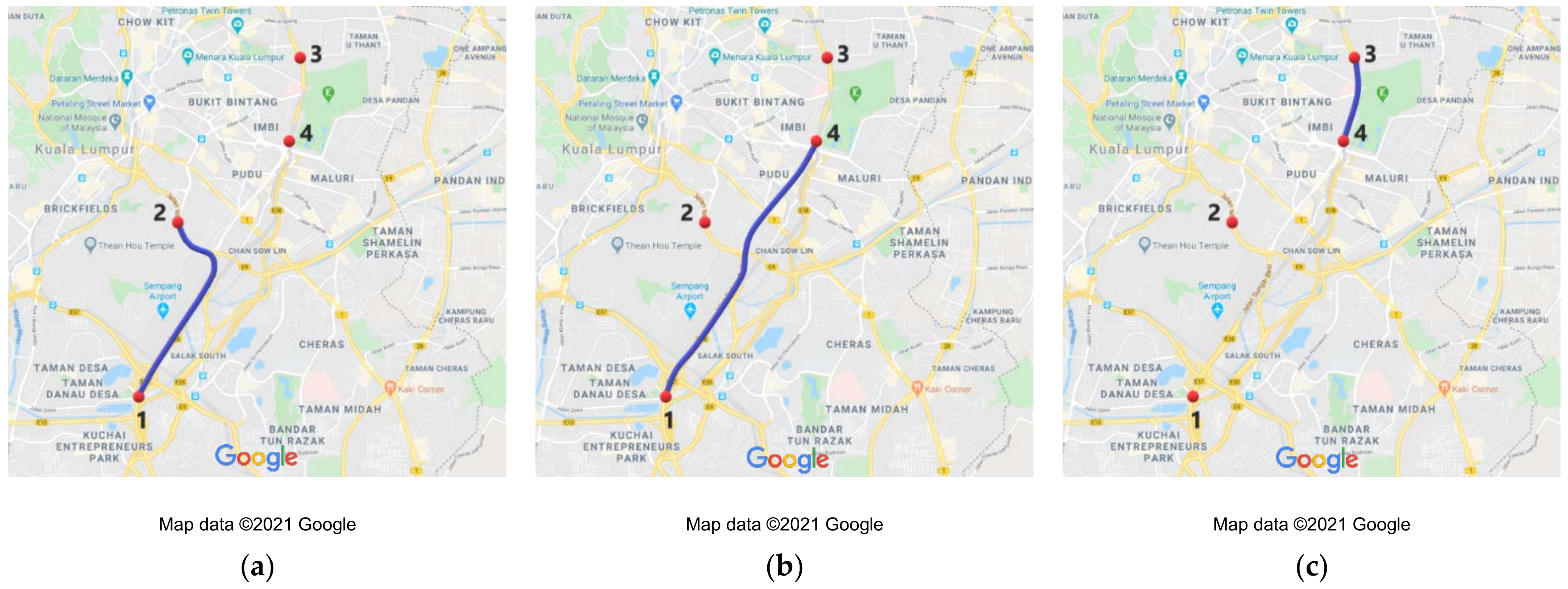
The data analyzed in this study is from an urban road network located near the Kuala Lumpur City Center (KLCC). There are skyscrapers in the area, including the Petronas Twin Towers, and many shopping centers, hotels, and business offices. Four MAC address sensors were installed at this road network to measure travel time. Sensor 1 is on the KL-Seremban Highway, Sensor 2 is on Istana Road, Sensor 3 is close to the U.S. Embassy on Tun Razak highway, and Sensor 4 is on Yew Road. These sensors collected the travel time data at three different routes. Figure 2 shows the locations of the sensors and the three routes.

To facilitate discussion, Route A is the route between sensors 1 and 2. Route B is between sensors 1 and 4. Route C is between sensors 4 and 3.

Table 2. Route information.

Route	Length (m)	No. of Segments	Connected Sensors	No. of Travel Time Observations
Route A	3880	2	1 and 2	89,225
Route B	5690	3	1 and 4	37,320
Route C	1410	1	4 and 3	117,114

presents the route information.

Route A comprises two segments; the first segment is a part of the KL-Seremban Expressway, and the second is Istana Road. Route B has three segments, a portion of the KL-Seremban Expressway, Sungai Besi Road, and Yew Road. Route C is a part of Tun Razak highway.

3.3. Data Collection

The traffic data used in this study were collected in 2018 by Integrated Transportation Solutions Sdn. Bhd. (ITSSB) under the Proof-of-Concept (PoC) project of the Advanced Traffic Information System (ATIS). This project is a collaboration with the Integrated Transport Information System (ITIS), DBKL. ITSSB collects the travel time data by developing a system that anonymously detects, transmits, records, matches, and analyzes the MAC address sent out periodically by smartphones via Wi-Fi to measure travel time. This study employed a part of the millions of MAC address data collected during the PoC project.

3.4. Data Description

The data description using the MAC address data for lane-splitting based on the actual situation contains a high percentage of motorcycles have never been reported. This section presents actual MAC address datasets in Malaysia to demonstrate the impact of lane-splitting on the travel time pattern. The presented datasets contain raw matched MAC address data before applying any filtering algorithm.

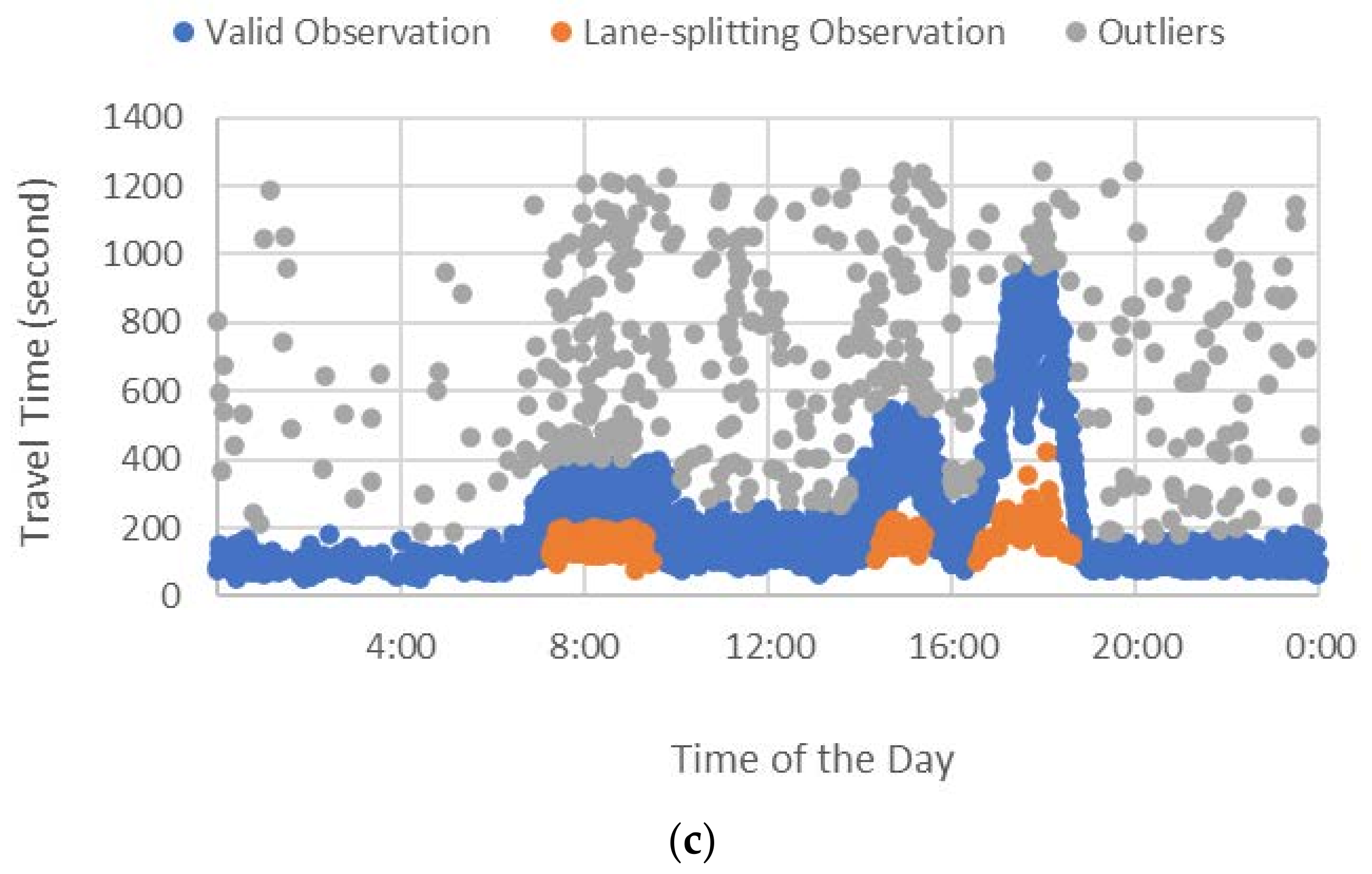
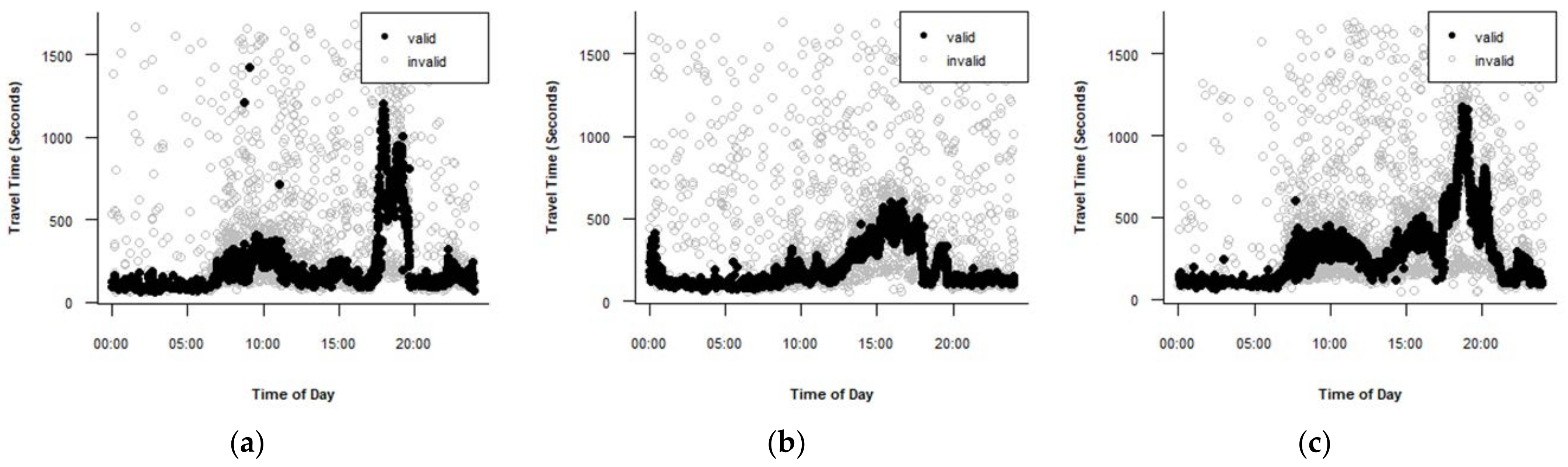
The travel time dataset for the study area is categorized into three observations: valid, outliers, and lane-splitting. Figure 3 presents the travel time datasets for Routes A, B, and C. In the figure, the blue points are the valid observations, the gray points are outliers, and the orange points are lane-splitting observations. The data was manually classified based on the authors’ experience. Figure 3a shows the travel times for Route A. The differences between the three categories are apparent for this route. Figure 3b shows the datasets for Route B. This route has much fewer outliers and lane-splitting data because it is longer and has many intersections. It is hard to filter this type of travel time dataset. Figure 3c presents the travel time observations for Route C. The figure shows a small gap between the lane-splitting and valid observations during the morning peak hour. However, the evening peak hour exhibits a significant difference between the lane-splitting observations and the valid observations. Based on the comparison between the morning peak hour and evening peak hour, the observations in the morning peak hour that are less than 200 s are considered lane-splitting.

To notice the difference in travel time between passenger vehicles and motorcycles,

Table 3. Average travel time for Passenger vehicles and motorcycles.

Time	Route A			Route B			Route C
	Average Travel Time (Second)		% Difference	Average Travel Time (Second)		% Difference	Average Travel Time (Second)		% Difference
	Passenger Vehicles	Motorcycles		Passenger Vehicles	Motorcycles		Passenger Vehicles	Motorcycles
8:00–8:09	697	309	55.65	909	381	58.09	250	154	38.31
8:10–8:19	669	270	59.64	950	375	60.48	274	151	44.89
8:20–8:29	616	273	55.59	1018	423	58.46	265	158	40.45
8:30–8:39	571	248	56.64	1217	436	64.17	281	156	44.45
8:40–8:49	505	272	46.07	1203	412	65.76	303	154	48.98
8:50–8:59	411	229	44.34	860	320	62.79	297	169	42.97

presents average travel time for passenger vehicles and motorcycles during morning peak period from 8:00 to 9:00. It is clear that the difference between passenger vehicles and motorcycles is very high for all routes.

3.5. Data Analysis

This study used extensive empirical travel time data from three routes to validate the performance of several filtering algorithms in detecting outliers and lane-splitting observations. The evaluated algorithms are the percentile algorithm, mean absolute deviation algorithm, TransGuide algorithm, Dion and Rakha algorithm (version 1 and 2), and Jang algorithm. The literature review section has presented the equations for each algorithm. Evaluation of the filtering algorithms was done in two stages to identify the most appropriate algorithm and the parameters for each route. This study used the R software to analyze the effectiveness of the algorithms and to make the calculations.

Stage 1: Validation of the Previous Filtering Algorithms

The validation of the algorithms used the travel time datasets for the three routes between 00:00 and 23:59 on 28 May 2018. This day was selected because it is a weekday. There are considerable amounts of lane-splitting observations within the datasets of this day for the three routes. The values of the algorithm parameters were calibrated using a trial-and-error method to identify the best performance of each algorithm. The assessment was conducted by observing the performance of each algorithm and comparing its performance with other algorithms using graphs. In addition, the mean absolute relative error (MARE) was used as a numerical indicator to compare the algorithms’ performances.

$$MARE=\frac{1}{n}{\displaystyle \sum }_{t=1}^n\frac{\left|x\left(t\right)-y\left(t\right)\right|}{x\left(t\right)}$$

(27)

where $n$ is the number of samples. $x\left(t\right)$ is the average travel time from ground truth data (the valid observations in Figure 3) at collection interval $t$ (five minutes), and $y\left(t\right)$ is the average travel time from a filtering algorithm at the collection interval $t$ (five minutes).

Travel time data collected by MAC addresses can be used as ground truth for intelligent transportation system applications [36]. In this study, the ground truth was extracted manually as Moghaddam and Hellinga [20] did in their study.

Stage 2: Sensitivity Analysis of the Algorithm Parameters

The best algorithm for each route was applied to datasets from ten days to verify the sensitivity of the algorithm parameters on different days. On the days that showed unaccepted results, the parameters were calibrated to determine the capability of the best algorithm to filter the data from all days. The parameters calibration was done using a trial-and-error method. The mean absolute relative error (MARE) was used as a numerical indicator to compare the algorithms’ performance before and after calibration.

4. Results and Discussion

4.1. Validation of the Previous Filtering Algorithm

The outlier detection algorithms discussed in the literature review section were applied to the travel time datasets for routes A, B, and C. The algorithms are percentile algorithm, mean absolute deviation algorithm, TransGuide algorithm, Dion and Rakha algorithm, and Jang algorithm. The validation used the travel time dataset from 00:00 to 23:59 on 28 May 2018.

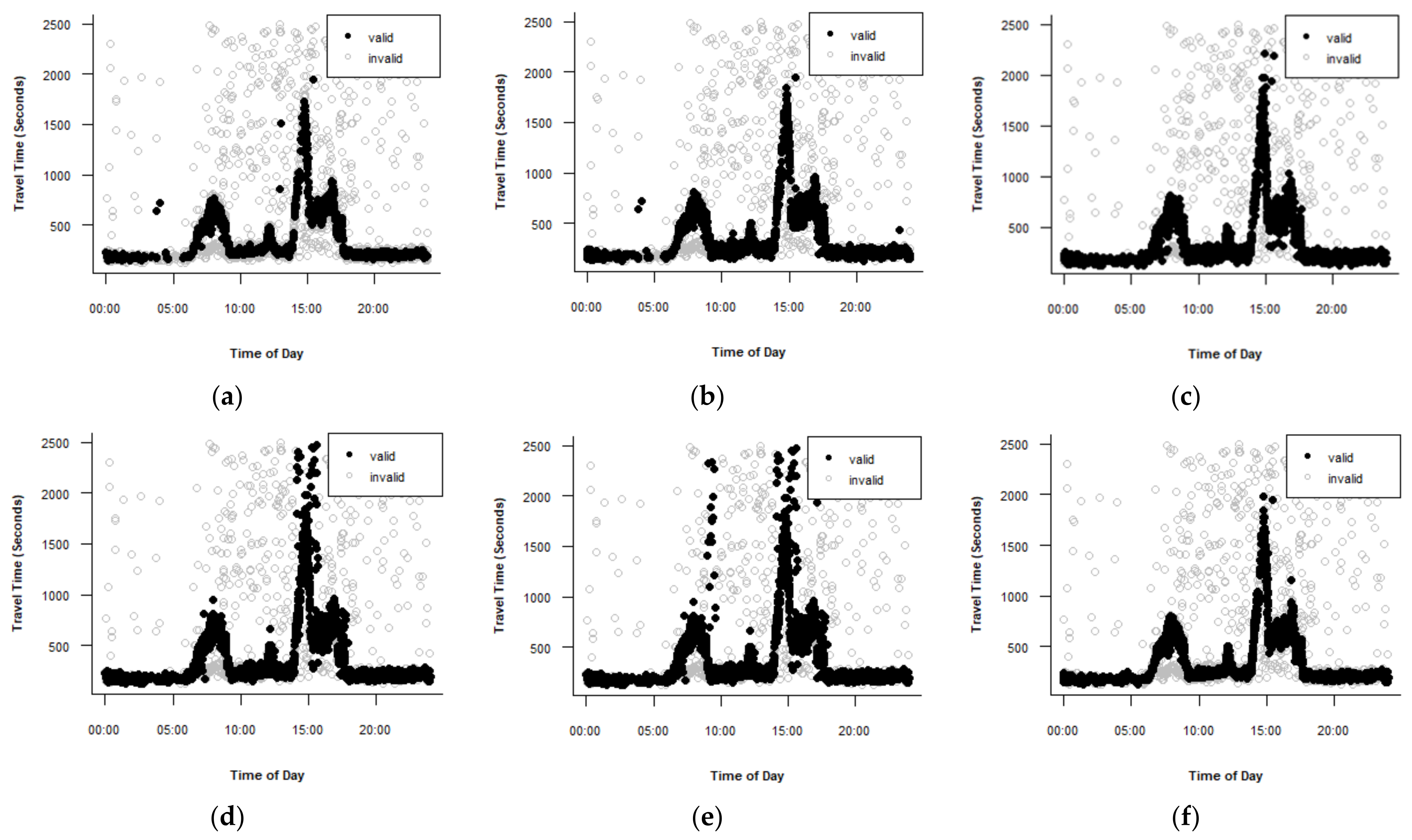
Figure 4 shows the results for Route A. Figure 4a presents the valid data after applying the percentile algorithm using the 25th percentile as the lower limit and the 75th percentile as the upper limit. The algorithm detects lane-splitting observations and most lane-splitting data but removed a significant number of valid observations. proposed using the 10th percentile as the lower limit and the 90th percentile as the upper limit. However, these limits did not result in a good performance. The mean absolute deviation algorithm with a validity range of $M_e\pm 3 MAD$ proposed by could not identify the lane-splitting data for the morning and evening peak hours and failed to detect a significant number of outliers. Thus, the validity range was modified to $M_e\pm 0.8 MAD$. This modification has a positive impact on the performance of the test, as shown in Figure 4b, even though it removed a significant number of valid observations. Figure 4c presents the result of using the TransGuide algorithm with $l_{th}$ = 0.5. This algorithm did not detect lane-splitting data at the onset of the morning peak hour and in the middle of the evening peak hour. Figure 4d shows the behavior of the Dion and Rakha version 1 algorithm. The parameter values that produced the best results are $\beta$ = 0.5, $n_{\sigma }$ = 2.5, and a time window of five minutes. The algorithm did not eliminate several lane-splitting observations in the morning and evening peak periods and failed to detect many outliers in the evening peak periods. Figure 4e shows the performance of the Dion and Rakha version 2 algorithm. The adopted parameters values are $\beta$ = 0.5, $n_{\sigma }$ = 2.5, time window of five minutes, n skips = 10. Version 2 showed worse performance than version 1. proposed using $\alpha$ = 0.35, $\beta$ = 3, and $\gamma$ = 0.3 in his algorithm. However, these values did not produce good results. This study changed the values to $\alpha$ = 1, $\beta$ = 1.5, and $\gamma$ = 0.3. The best algorithm for route A is the Jang algorithm.

Figure 5 shows the performances of the algorithms for Route B. Figure 5a shows the result of applying the percentile test using the 25th percentile as the lower limit and the 75th percentile as the upper limit. The result is not satisfactory. Figure 5b shows that the mean absolute deviation algorithm with a validity range of $M_e\pm 0.3 MAD$ did not detect all lane-splitting observations in the morning peak hour. Figure 5c presents the result of using the TransGuide algorithm with $l_{th}$ = 0.3. This algorithm is the best for Route B because it efficiently detects the lane-splitting data and outliers. Figure 5d,e show the behavior of Dion and Rakha version 1 and version 2 algorithms, respectively. Both algorithms showed poor performance in detecting outliers. Figure 5f shows the behavior of the Jang algorithm using the parameters values $\alpha$ = 0.3, $\beta$ = 1, and $\gamma$ = 0.3. The algorithm did not remove all lane-splitting observations in the morning peak period but removed a significant number of valid travel time observations in the morning peak hour.

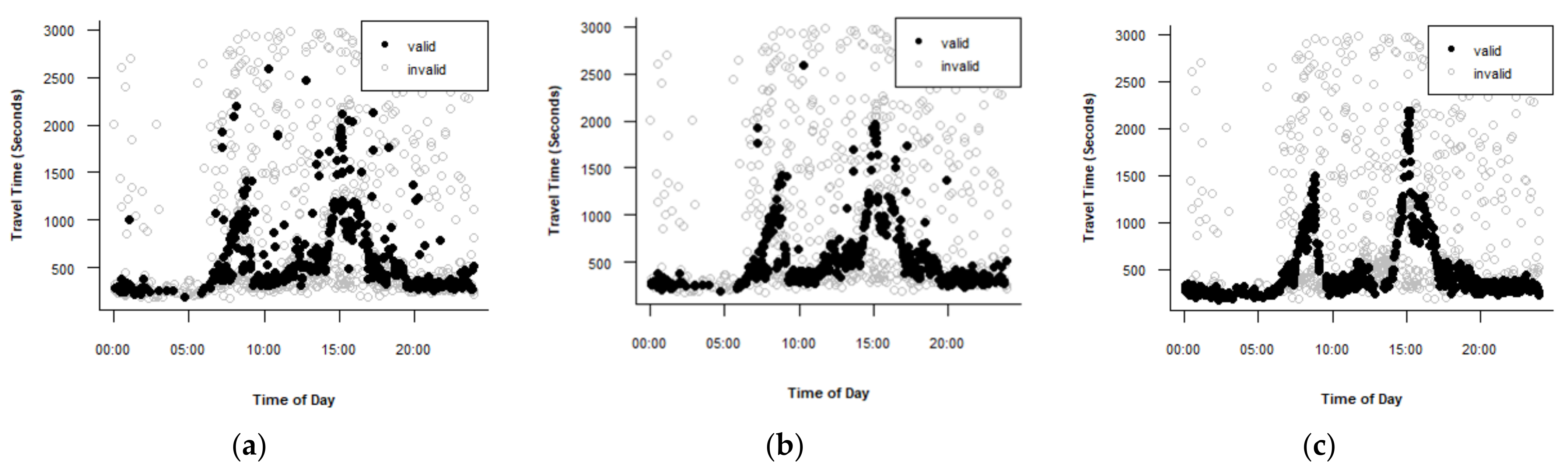
Figure 6 shows the results for Route C. Figure 6a shows the result for the percentile algorithm using the 25th percentile as the lower limit and the 75th percentile as the upper limit. The algorithm showed a good performance detecting lane-splitting data and outliers but removed a significant number of valid observations. Figure 6b shows that the mean absolute deviation algorithm with a validity range of $M_e\pm 0.5 MAD$ showed good performance detecting lane-splitting data and outliers but removed a significant number of valid observations. Figure 6c shows that the TransGuide algorithm with $l_{th}$ = 0.6 did not detect the lane-splitting data. The Dion and Rakha version 1 and version 2 algorithms failed to remove the lane-splitting data in the morning peak period and did not detect a considerable number of outliers, as shown in Figure 6d,e, respectively. Figure 6f shows the performance of the Jang algorithm with $\alpha$ = 0.5, $\beta$ = 1, and $\gamma$ = 0.3. This algorithm showed excellent performance in detecting the lane-splitting observations and outliers. Therefore, the Jang algorithm is the best for Route C.

Table 4. MARE values for the three routes for 28 May.

Filtering Algorithm	Mean Absolute Relative Error (MARE)
	Route A	Route B	Route C
Percentile algorithm	0.132	0.392	0.158
Mean absolute deviation algorithm	0.123	0.386	0.140
TransGuide algorithm	0.050	0.129	0.078
Dion and Rakha algorithm Version 1	0.049	0.313	0.082
Dion and Rakha algorithm Version 2	0.052	0.226	0.083
Jang algorithm	0.028	0.153	0.050

presents the MARE values for the three routes for 28 May. The algorithm with the smallest MARE value is the best, indicating that this algorithm has minimum error relative to the ground truth data. The table shows that the Jang algorithm is the best for Routes A and C, while the TransGuide algorithm is the best for Route B. This finding affirms the conclusions drawn from the discussion of Figure 4, Figure 5 and Figure 6.

4.2. Sensitivity Analysis of the Algorithm Parameters

The travel time data from ten days were used to determine if the best algorithm parameters require daily calibration to achieve the best performance or if the parameters used in the previous section are suitable for all days. The ten days are 2, 5, 8, 11, 14, 17, 20, 23, 26, and 29 May 2018. The 2, 8, 14, 17, and 23 May are weekdays; 5, 20, and 26 May are weekends; 11 May is an election day; and 29 May is a holiday. This section tested only the algorithm that showed the best performance for each route.

The algorithm parameters are sensitive for different days if any day shows unacceptable performance, indicating that algorithm parameters require calibration on the days with unaccepted performance. The calibration involves modifying the values of algorithm parameters using a trial-and-error method to ensure the algorithm achieves the best performance. This step checks the ability of the algorithm to filter the data from all days.

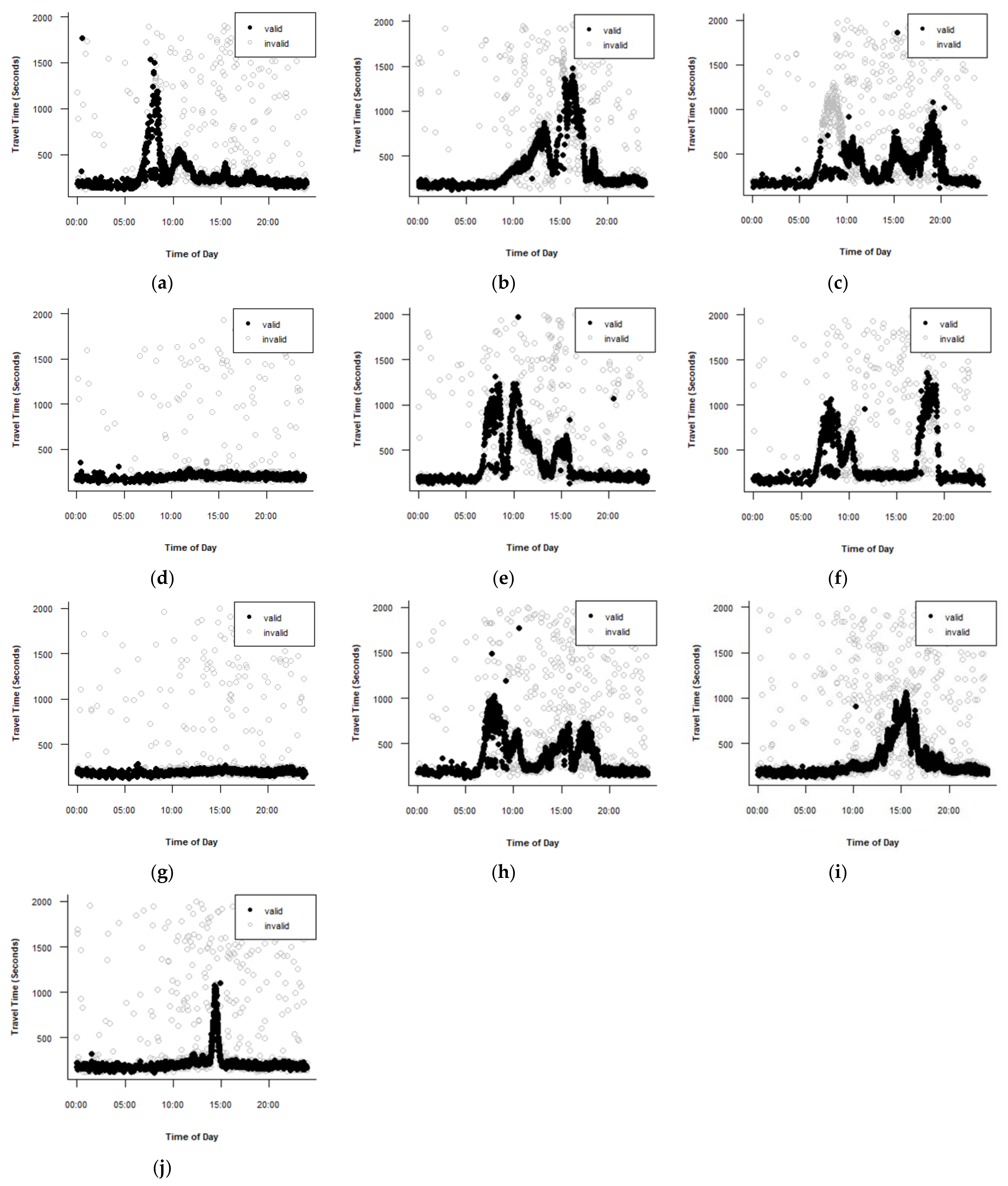
The Jang algorithm with $\alpha$ = 1, $\beta$ = 1.5, $\gamma$ = 0.3, and $t_W$ = 5 showed the best performance for Route A for the 28 May travel time dataset. The Jang algorithm with these parameters was applied for the ten days, and Figure 7 shows the results. Figure 7a,c,e,f,h show the datasets with poor performance because considerable amounts of lane-splitting observations during morning peak period remained after filtration. It is worth noting that these figures are for the weekdays. Therefore, the Jang algorithm parameters for Route A are sensitive for datasets from different days, and it is essential to make daily calibration of the parameters to obtain acceptable results.

The Jang algorithm parameters for the datasets that showed unacceptable results in Figure 7 were calibrated using a trial-and-error method.

Table 5. MARE values for route A.

Date	Mean Absolute Relative Error (MARE)
	Entire Day		8:00–9:00
	Before Calibration	After Calibration	Before Calibration	After Calibration
2 May	0.051	0.040	0.319	0.069
8 May	0.100	0.063	0.779	0.027
14 May	0.040	0.033	0.205	0.031
17 May	0.050	0.039	0.181	0.038
23 May	0.037	0.029	0.207	0.042

presents the MARE values for route A before and after calibration for the days that need to be calibrated. The MARE values for entire day after calibration were less than before calibration for all days, indicating that the calibration of the parameters improved the performance of the Jang algorithm. For the morning peak period, the amounts of lane-splitting observations before calibration were considerable for all days as shown in Figure 7a,c,e,f,h. As such, the MARE values for 8:00–9:00 before calibration were high as presented in Table 5. The MARE values for 8:00–9:00 after calibration were much less than before calibration for all days. This indicates that the calibration of the parameters highly improved the performance of the Jang algorithm during this period.

The Jang algorithm has four parameters, $\alpha$, $\beta$, $\gamma$, and $t_W$.

Table 6. Parameter values after calibration for Route A.

Date	$\mathit{\alpha }$	$\mathit{\beta }$	$\mathit{\gamma }$	${\mathit{t}}_{\mathit{W}}$
2 May	0.5 1	1 1	0.3	5
8 May	0.5 1	0.5 1	0.3	1 1
14 May	0.5 1	1 1	0.3	5
17 May	0.5 1	1 1	0.3	5
23 May	0.5 1	1 1	0.3	5
Value before calibration	1	1.5	0.3	5

¹ The parameter value is different from the value before calibration.

shows the values of the Jang algorithms’ parameters after calibration for the days that showed unacceptable performance before calibration for route A. The $\alpha$, $\beta$, and $t_W$ are sensitive, while $\gamma$ is insensitive. Four of five days have the same parameters, indicating that, after calibration, there are two new parameters sets, $\alpha$ = 0.5, $\beta$ = 0.5, $\gamma$ = 0.3, and $t_W$ = 1 for 8 May. The other parameters set, $\alpha$ = 0.5, $\beta$ = 1, $\gamma$ = 0.3 and $t_W$ = 5, are for 2, 14, 17, and 23 May. $t_W$ is different for just one day, indicating the sensitivity of $t_W$ is less than $\alpha$ and $\beta$.

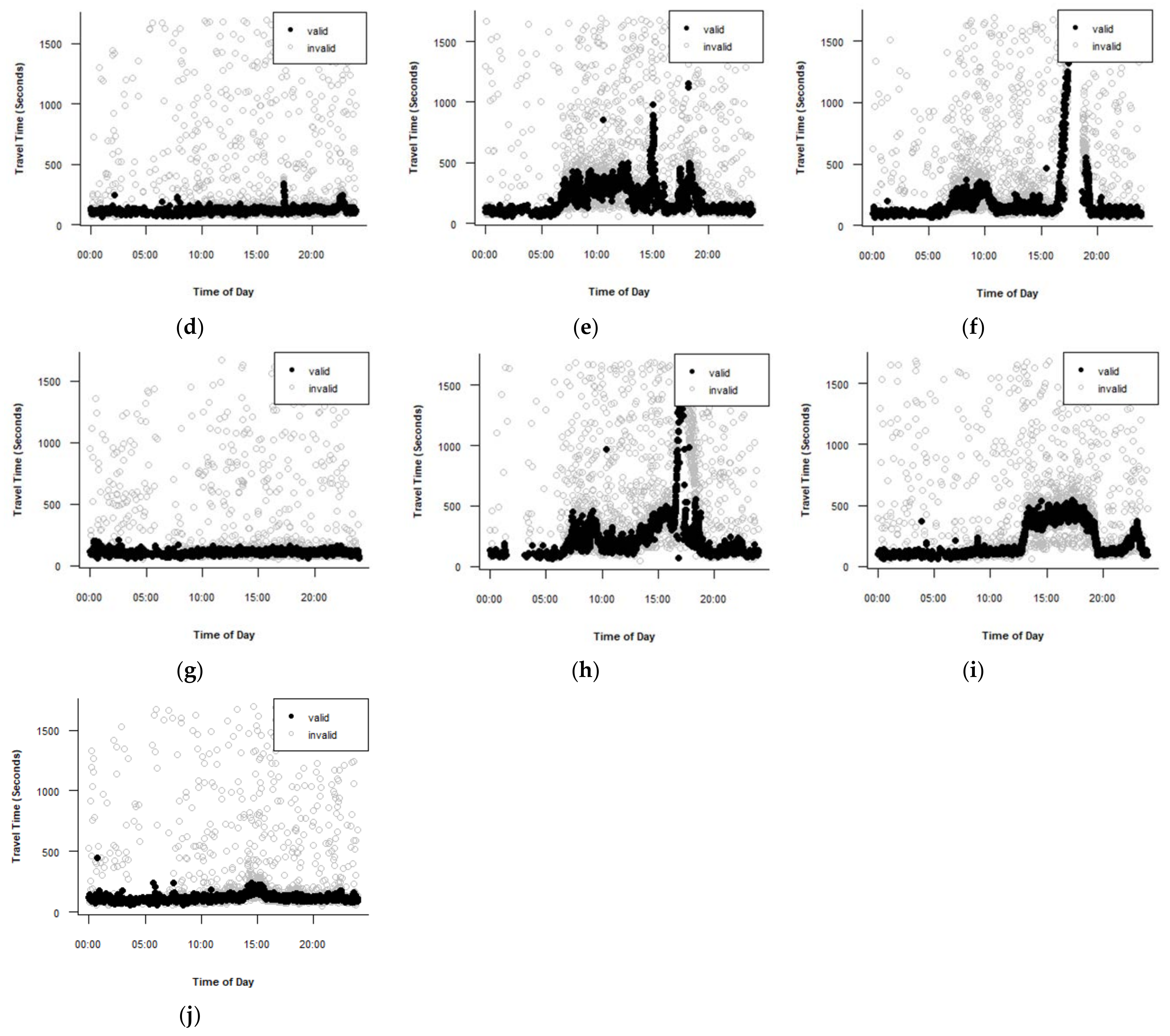
The TransGuide algorithm with $l_{th}$ = 0.3 and $t_W$ = 5 is the best algorithm for filtering the datasets for Route B for 28 May. The data for the ten days were filtered using the TransGuide algorithm with $l_{th}$ = 0.3 and $t_W$ = 5. Figure 8 shows the performance of the TransGuide algorithm for Route B for the ten days. Figure 8a–c,e,h,i show the datasets with poor performance. These datasets represent four weekdays and two weekends. Clearly, the TransGuide algorithm failed to follow the valid observations at the peak periods. As such, the parameters of the TransGuide algorithm for Route B are sensitive for datasets from different days and required calibration for each day.

Table 7. MARE values for route B.

Date	Mean Absolute Relative Error (MARE)
	Before Calibration	After Calibration
2 May	0.318	0.081
5 May	0.227	0.036
8 May	0.301	0.067
14 May	0.329	0.030
23 May	0.137	0.069
26 May	0.357	0.034

presents the MARE for route B before and after calibration for the days that need to be calibrated. The values of MARE for all days after calibration were much less than before calibration, indicating that the calibration of the parameters highly improved the performance of TransGuide algorithm.

Table 8. Parameter values after calibration for Route B.

Date	${\mathit{l}}_{\mathit{t}\mathit{h}}$	${\mathit{t}}_{\mathit{W}}$
2 May	0.5 1	5
5 May	0.5 1	5
8 May	0.35 1	4 1
14 May	0.45 1	5
23 May	0.3	6 1
26 May	0.5 1	4 1
Value before calibration	0.3	5

¹ The parameter value is different from the value before calibration.

shows the values of the TransGuide algorithms’ parameters after calibration for the days that showed unacceptable performance before calibration for Route B. Both parameters, $l_{th}$ and $t_W$, are sensitive. There are five new parameters sets after the calibration. The best parameters for 2 and 5 May are $l_{th}$ = 0.5 and $t_W$ = 5. The remaining days have different parameter sets.

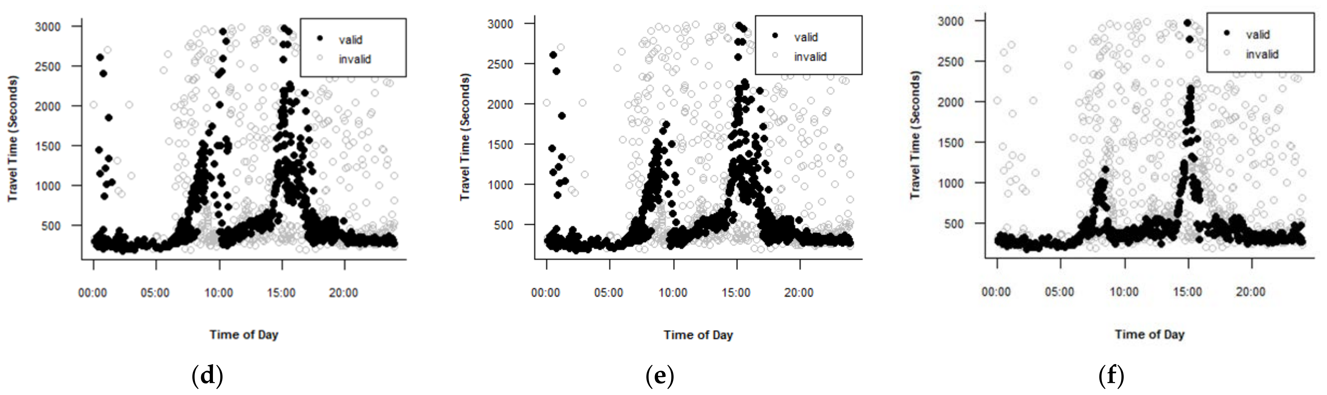
The Jang algorithm with $\alpha$ = 1, $\beta$ = 1, $\gamma$ = 0.3, and $t_W$ = 5 is the best algorithm for the Route C travel time data for 28 May and was applied for the ten days. Figure 9 shows the Jang algorithm performance for Route C for the ten days. Figure 9h shows the poor performance for the data for 23 May, which is a weekday. The Jang algorithm parameters are sensitive because one dataset for Route C showed poor performance. Therefore, the parameters require daily calibration to ensure good performance.

Table 9. MARE values for route C.

Date	Mean Absolute Relative Error (MARE)
	Entire Day		17:00–18:00
	Before Calibration	After Calibration	Before Calibration	After Calibration
23 May	0.104	0.077	0.544	0.039

presents the MARE for route C before and after calibration for 23 May. The MARE value after calibration was less than before calibration, indicating that the calibration of the Jang algorithm parameters improved the performance of the Jang algorithm. For the evening peak period, the number of lane-splitting observations before calibration was considerable as shown in Figure 9h. As such, the MARE value for 17:00–18:00 before calibration (0.544) was very high as presented in Table 9. The MARE value for 17:00–18:00 after calibration (0.039) was much less than before calibration (0.544). This indicates that the calibration of the parameters highly improved the performance of the Jang algorithm during this period.

Table 10. Parameter values after calibration for Route C.

Date	$\mathit{\alpha }$	$\mathit{\beta }$	$\mathit{\gamma }$	${\mathit{t}}_{\mathit{W}}$
23 May	0.5 1	1	0.3	5
Value before calibration	1	1	0.3	5

¹ The parameter value is different from the value before calibration.

shows the values of the Jang algorithm’s parameters after calibration for the days that showed unacceptable performance before calibration for Route C. The table shows that $\alpha$ is sensitive, but the other parameters are insensitive. Only one parameter for one day is sensitive for Route C. Therefore, the sensitivity of Route C is lower than Routes A and B.

Table 11. Summary of the evaluation of filtering algorithms.

Route	The Best Algorithm	No. of Days with Poor Performance before Calibration	No. of New Parameter Sets after Calibration
A	Jang	5	2
B	TransGuide	6	5
C	Jang	1	1

summarizes the evaluation of the filtering algorithms and the sensitivity of the algorithm parameters. The Jang algorithm is the best for Routes A and C, while the TransGuide algorithm is the best for Route B. The number of days with poor performance before calibration, and the number of new parameter sets after calibration are used to compare the routes in terms of the sensitivity of the algorithm’s parameters. Route C is less sensitive, with only one day of poor performance before calibration. Route B is more sensitive than Routes A and C because it has the highest number of days with poor performance before calibration and the highest number of new parameter sets after calibration. Because Routes A and C are less sensitive than Route B, the Jang algorithm is less sensitive than the TransGuide algorithm.

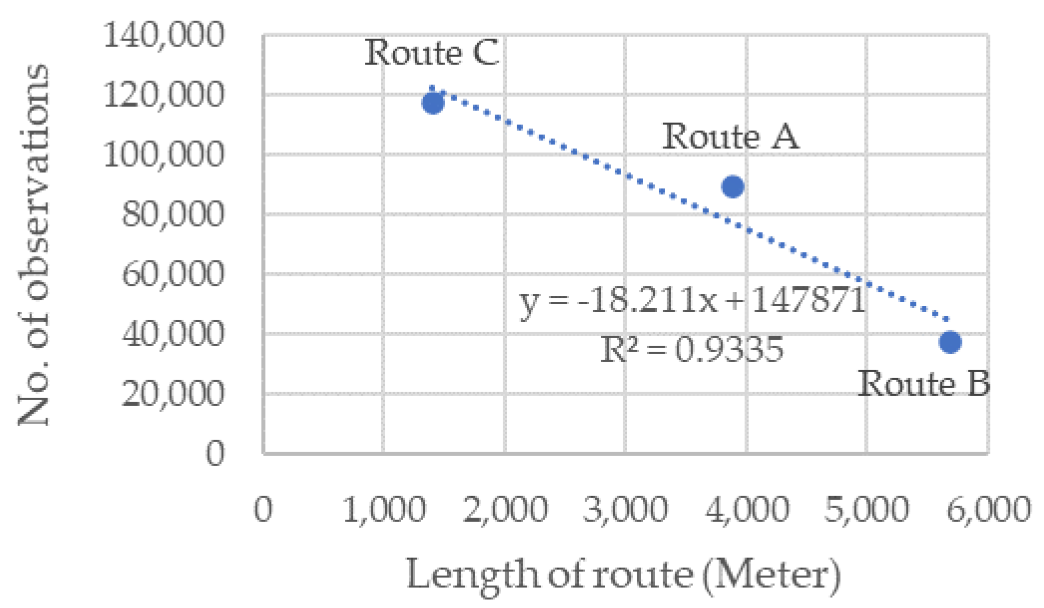
The route length is the distance between the two Wi-Fi sensors at the start and the end of the route. The Pearson correlation coefficient, effect size, and coefficient of determination are calculated to test the relationship of the distance between the sensors and the number of travel time observations.

Table 12. Results of the correlation test.

Pearson Correlation Coefficient ®	Effect Size (d)	Coefficient of Determination (R2)
−0.966	−7.47	0.93

shows that the effect size (d) is compatible with the Coefficient of Determination (R²) since R² (0.93) and d (−7.47) are very large based on Cohen’s standard [37]. In addition, the slope of the trend line in Figure 10 and the sign of d are negative. Thus, there is a very large negative correlation between the distance between the sensors and the number of observations. This indicates that the distance between the sensors has to be shortened to obtain more observations. Based on Table 11 and Figure 10, it can be concluded that the increase in the number of observations makes the Jang algorithm the best filtering algorithm. Jang algorithm is the best algorithm for Routes A and C because they have more observations than Route B.

Concerning the sensitivity of the algorithm parameters, Route C is less sensitive than Routes A and B because it has the highest number of observations. Route B is more sensitive than Routes A and C and has the lowest number of observations. Route A is more sensitive than Route C but less sensitive than Route B. Route A has fewer observations than Route C but more observations than Route B. Thus, the algorithms’ parameter sensitivity is inversely proportional to the number of observations. This means that the algorithms are highly sensitive at low number of observations, making the filtration is difficult. This conclusion conforms with the argument of Dion and Rakha [31] about the difficulties of filtering travel time datasets that have low sampling rate, especially the difficulty of tracking sudden changes in traffic conditions. Given the inverse proportion of the distance between sensors (or the route length) with the number of observations, the sensitivity of the algorithm parameters is directly proportional to the distance between sensors.

5. Conclusions

This paper has addressed the methods for filtering the travel time data for Malaysian roads with common lane-splitting situations. The two main problems with the datasets collected by MAC address are the outliers and lane-splitting observations. The literature proposed many travel time filtering algorithms for removing outliers from travel time datasets. Evaluation of these algorithms by considering lane-splitting yielded the following finding.

• The Jang algorithm and TransGuide algorithm are effective in filtering the outliers and lane-splitting data. The Jang algorithm is the best algorithm for Routes A and C, while the TransGuide algorithm is the best algorithm for Route B.
• The parameters of the Jang and TransGuide algorithms are sensitive for different days and can be used after daily parameter calibration.
• Since Routes C and A are less sensitive than Route B, the Jang algorithm is less sensitive than the TransGuide algorithm.
• The distance between sensors and the number of observations for the study area are inversely proportional.
• It can be concluded that an increase in the number of observations makes the Jang algorithm the best filtering algorithm because the Jang algorithm is the best algorithm for Routes A and C, which have more observations than route B.
• The sensitivity of the algorithm parameters is inversely proportional to the number of observations. Given the inverse proportion of the distance between sensors and the number of observations, the algorithms’ sensitivity is directly proportional to the distance between sensors.

In conclusion, even though there are many filtering algorithms, their usage is dependent on the characteristics of the travel time data. Two of the five well-known algorithms investigated in this study showed promising results. Even though the best two algorithms could filter the outliers and lane-splitting observations, they require considerable improvement to resolve the sensitivity issue. This will help to apply the filtration algorithms easily in real-time applications. In addition, it is recommended to use travel time data from more than three routes to investigate the statistical relationships in this study.

However, due to COVID-19, the authors could not collect recent traffic data due to Malaysia’s full and partial lockdowns. Undoubtedly, traffic is highly affected by these lockdowns. This was the main reason why the data in this research was archived data of the actual traffic condition of May 2018. Moreover, for the study area, the other traffic parameters such as traffic flow were not collected during May 2018.

References

- Gil Sander, F.; Blancas Mendivil, L.C.; Westra, R. Malaysia Economic Monitor: Transforming Urban Transport; The World Bank: Bangkok, Thailand, 2015. [Google Scholar]
- Wan, X.; Ghazzai, H.; Massoud, Y. Mobile crowdsourcing for intelligent transportation systems: Real-time navigation in urban areas. IEEE Access 2019, 7, 136995–137009. [Google Scholar] [CrossRef]
- Lu, Z.; Xia, J.; Wang, M.; Nie, Q.; Ou, J. Short-term traffic flow forecasting via multi-regime modeling and ensemble learning. Appl. Sci. 2020, 10, 356. [Google Scholar] [CrossRef] [Green Version]
- Shokoohyar, S.; Sobhani, A.; Sobhani, A. Impacts of trip characteristics and weather condition on ride-sourcing network: Evidence from Uber and Lyft. Res. Transp. Econ. 2020, 80, 100820. [Google Scholar] [CrossRef]
- Noor, R.M.; Rasyidi, N.B.G.; Nandy, T.; Kolandaisamy, R. Campus Shuttle Bus Route Optimization Using Machine Learning Predictive Analysis: A Case Study. Sustainability 2021, 13, 225. [Google Scholar] [CrossRef]
- Ministry of works Malaysia. Malaysian its Blueprint (2019–2023); Ministry of works Malaysia: Kuala Lumpur, Malaysia, 2019. [Google Scholar]
- Hao, Q.; Qin, L. The design of intelligent transportation video processing system in big data environment. IEEE Access 2020, 8, 13769–13780. [Google Scholar] [CrossRef]
- Vrbanić, F.; Ivanjko, E.; Kušić, K.; Čakija, D. Variable speed limit and ramp metering for mixed traffic flows: A review and open questions. Appl. Sci. 2021, 11, 2574. [Google Scholar] [CrossRef]
- Nguyen, D.D.; Rohács, J.; Rohács, D.; Boros, A. Intelligent total transportation management system for future smart cities. Appl. Sci. 2020, 10, 8933. [Google Scholar] [CrossRef]
- Peng, T.; Yang, X.; Xu, Z.; Liang, Y. Constructing an Environmental Friendly Low-Carbon-Emission Intelligent Transportation System Based on Big Data and Machine Learning Methods. Sustainability 2020, 12, 8118. [Google Scholar] [CrossRef]
- Musa, N.S.; Noor, N.M.M.; Marjan, J.M. The benefits of National Intelligent Transportation Management Centre (NITMC) establishment in Malaysia. In Proceedings of the IOP Conference Series: Materials Science and Engineering, Selangor, Malaysia; 2019; p. 012013. [Google Scholar]
- Martchouk, M.; Mannering, F.; Bullock, D. Analysis of freeway travel time variability using Bluetooth detection. J. Transp. Eng. 2011, 137, 697–704. [Google Scholar] [CrossRef]
- Long, K.; Yao, W.; Gu, J.; Wu, W.; Han, L.D. Predicting freeway travel time using multiple-source heterogeneous data integration. Appl. Sci. 2019, 9, 104. [Google Scholar] [CrossRef] [Green Version]
- Liu, Y.; Xia, J.C.; Phatak, A. Evaluating the Accuracy of Bluetooth-Based Travel Time on Arterial Roads: A Case Study of Perth, Western Australia. J. Adv. Transp. 2020. [Google Scholar] [CrossRef] [Green Version]
- Shokoohyar, S.; Sobhani, A.; Malhotra, R.; Liang, W. Travel Time Prediction in Ride-Sourcing Networks: A Case Study for Machine Learning Applications. J. Bus. Cases Appl. 2020, 26, 1–20. [Google Scholar]
- Guo, J.; Li, C.; Qin, X.; Huang, W.; Wei, Y.; Cao, J. Analyzing distributions for travel time data collected using radio frequency identification technique in urban road networks. Sci. China Technol. Sci. 2019, 62, 106–120. [Google Scholar] [CrossRef]
- Chen, Z.; Fan, W.D. Analyzing travel time distribution based on different travel time reliability patterns using probe vehicle data. International J. Transp. Sci. Technol. 2020, 9, 64–75. [Google Scholar] [CrossRef]
- Van Boxel, D.; Schneider, W.H., IV; Bakula, C. Innovative real-time methodology for detecting travel time outliers on interstate highways and urban arterials. Transp. Res. Rec. 2011, 2256, 60–67. [Google Scholar] [CrossRef]
- Moghaddam, S.S.; Hellinga, B. Evaluating the performance of algorithms for the detection of travel time outliers. Transp. Res. Rec. 2013, 2338, 67–77. [Google Scholar] [CrossRef]
- Moghaddam, S.S.; Hellinga, B. Algorithm for detecting outliers in Bluetooth data in real time. Transp. Res. Rec. 2014, 2442, 129–139. [Google Scholar] [CrossRef]
- Ouellet, J.V. Lane splitting on California freeways. In Proceedings of the Transportation Research Board 91st Annual Meeting, Washington, DC, USA, 22–26 January 2012. [Google Scholar]
- Rice, T.; Troszak, L.; Erhardt, T. Motorcycle Lane-Splitting and Safety in California; University of California Berkeley: Berkeley, CA, USA, 2015. [Google Scholar]
- Kurlantzick, A.; Krosner, B. Motorcycle Lane Splitting: A Literature Review; Ride to Work: Duluth, MN, USA, 2016. [Google Scholar]
- Beanland, V. Evaluation of the ACT Motorcycle Lane Filtering Trial; Centre for Human Factors and Sociotechnical Systems: Canberra, Australia, 2018. [Google Scholar]
- Beanland, V.; Pammer, K.; Sledziowska, M.; Stone, A. Drivers’ attitudes and knowledge regarding motorcycle lane filtering practices. In Proceedings of the 2015 Australasian Road Safety Conference, Queensland, Australia, 14–16 October 2015. [Google Scholar]
- Sperley, M.; Pietz, A.J. Motorcycle Lane-Sharing: Literature Review; Oregon Department of Transportation: Salem, OR, USA, 2010. [Google Scholar]
- Aupetit, S.; Espié, S.; Bouaziz, S. Naturalistic study of riders’ behaviour in lane-splitting situations. Cogn. Technol. Work 2015, 17, 301–313. [Google Scholar] [CrossRef]
- Lee, J. Vehicle Registrations in Malaysia Hit 28.2 Million Units. Available online: https://paultan.org/2017/10/03/vehicle-registrations-in-malaysia-hit-28-2-million-units/ (accessed on 10 January 2021).
- Clark, S.D.; Grant-Muller, S.; Chen, H. Cleaning of matched license plate data. Transp. Res. Rec. 2002, 1804, 1–7. [Google Scholar] [CrossRef]
- Southwest Research Institute. Automatic Vehicle Identification Model Deployment Initiative-System Design Document; Southwest Research Institute: San Antonio, TX, USA, 1998. [Google Scholar]
- Dion, F.; Rakha, H. Estimating dynamic roadway travel times using automatic vehicle identification data for low sampling rates. Transp. Res. Part B Methodol. 2006, 40, 745–766. [Google Scholar] [CrossRef]
- Jang, J. Outlier filtering algorithm for travel time estimation using dedicated short-range communications probes on rural highways. IET Intell. Transp. Syst. 2016, 10, 453–460. [Google Scholar] [CrossRef]
- Chen, S.; Wang, W.; van Zuylen, H. A comparison of outlier detection algorithms for ITS data. Expert Syst. Appl. 2010, 37, 1169–1178. [Google Scholar] [CrossRef]
- Wu, Z.; Wu, Z.; Rilett, L.R. Innovative nonparametric method for data outlier filtering. Transp. Res. Rec. 2020, 2674, 167–176. [Google Scholar] [CrossRef]
- Google. Kuala Lumpur Roads. Available online: https://www.google.com/maps/@3.1310283,101.7046947,14.32z (accessed on 10 January 2021).
- Haghani, A.; Hamedi, M.; Sadabadi, K.F.; Young, S.; Tarnoff, P. Data collection of freeway travel time ground truth with bluetooth sensors. Transp. Res. Rec. 2010, 2160, 60–68. [Google Scholar] [CrossRef]
- Cohen, J. Statistical Power Analysis for the Behavioral Sciences; Academic press: Cambridge, MA, USA, 2013. [Google Scholar]