Detecting All Non-Dominated Points for Multi-Objective Multi-Index Transportation Problems

Abstract

Multi-dimensional transportation problems denoted as multi-index are considered as the extension of classical transportation problems and are appropriate practical modeling for solving real–world problems with multiple supply, multiple demand, as well as different modes of transportation demands or delivering different kinds of commodities. This paper presents a method for detecting the complete nondominated set (efficient solutions) of multi-objective four-index transportation problems. The proposed approach implements weighted sum method to convert multi-objective four-index transportation problem into a single objective four-index transportation problem, that can then be decomposed into a set of two-index transportation sub-problems. For each two-index sub-problem, parametric analysis was investigated to determine the range of the weights values that keep the efficient solution unchanged, which enable the decision maker to detect the set of all nondominated solutions for the original multi-objective multi-index transportation problem, and also to find the stability set of the first kind for each efficient solution. Finally, an illustrative example is presented to illustrate the efficiency and robustness of the proposed approach. The results demonstrate the effectiveness and robustness for the proposed approach to detect the set of all nondominated solutions.

1. Introduction

The conventional transportation problem is a two-index transportation problem that can be represented as a special mathematical modelling which comprises a cost function subject to certain constraints. In classical methods, transporting costs from s sources to d destinations are to be minimized [1,2,3,4]. Multi-dimensional transportation problems denoted as multi-index are the extension of classical transportation problems and are appropriate practical modelling for solving real-world transportation problems with multiple supply, multiple demand as well as networks using diverse modes of transportation demands or delivering different kinds of commodities [5,6].

Many researchers have studied the practical investigation of multi-index transportation problem in optimization, mathematical modelling, and in industry. Wang et al. [7] implemented a decomposition method based on the sequential modification of the optimality criterion for dealing with the classical three-index transportation problem. They investigated the solutions of the transportation problem with a linear and quadratic objective function. Zitouni et al. [8] investigated a numerical study of a capacitated transportation problem with four subscripts (four indices) in order to realize a practical software to meet real needs. Manal et al. [9] presented an adaption of a classical crisp method to solve the four-index fuzzy transportation problem. Also, they found the optimal solution by improvement of the initial solution. Pham el al. [10] aimed to find a solution on the minimum transportation cost for the four-index transportation problem. They also developed an exact method to solve this problem with real variables. Skitsko et al. [11] developed an approach for applying the genetic algorithm for solving four-index transportation problems using evolutionary algorithms. Also, their conclusions promoted the application of the genetic algorithm for solving four-index transportation. In [12], the authors aimed to find a solution for the minimum transportation cost of the four-index transportation problem. They also developed a resolution method based on the coupling of a mathematical model, an algorithm, and a database.

In [13], the researchers implemented the modified distribution method to obtain an optimal solution for the four-index transportation problem. Djamel et al. [14] focused on the theoretical study and numerical solution of a capacitated four-index transportation problem, and constructed an algorithm for solving the problem. In [15], researchers investigated construction and algebraic formulation of a four-index transportation problem. The researchers in [16] dealt with bi-objective multi-index bulk transportation problem as an extension of a single objective multi-index bulk transportation problem. Their method was presented to minimize time and cost simultaneously. In [17], researchers dealt with the multi-index transportation problem, their method considering the indeterminacy of the demand parameters and the cost of cargo transportation. They developed a software application to solve a multi-index distribution problem with fuzzy parameters. In [18], an approach based on the study of reducibility of the multi-index transport problems to that of seeking a flow on the network was proposed. Pasa [19] aimed through his research to model the multi-index transportation problem which implies solving the non-linear problem with a non-linear objective function and linear restrictions. In [20], a fuzzy multi-index bi-criteria fixed charge bottleneck transportation problem was considered, and for the first time all parameters were taken as trapezoidal fuzzy numbers. El-Shorbagy et al. [21] presented an improved genetic algorithm for dealing with a multi-objective fuzzy multi–index multi-objective transportation problem (FM-MOTP). In [22], researchers presented the application of fuzzy theory for handling a multi-objective multi-index real-world transportation problem. In [5], the authors investigated a constrained multi-index transportation problem with axial constraints, and with bounds on source availabilities, on destination demands, and various types of commodities. In [23], researchers investigated a constrained multi−objective multi−index transportation problem, in which demands, supplies, and requirements were represented by triangular fuzzy numbers. The research in [24] represents a generalized nonlinear bi-objective multi-index transportation problem.

In this paper, we intend to locate the set of all efficient solutions (nondominated solutions) of the multi-objective multi-index transportation problem, which is considered a large-scale problem due to the curse of dimensionality. The proposed algorithm implements a weighted sum method to transform the multi-objective problem into a single objective problem; then the decomposition technique was applied to decompose the problem to a smaller-size two-index transportation sub-problem. Stability analysis for the weighted parameters was applied to determine its range to retain the optimal solution. Finally, a numerical illustrative example is presented for the sake of illustration.

The proposal is arranged as follows. Section 2 introduces problem formulation of the transportation problem with different dimensions. Section 3 discusses the theoretical preliminaries. Section 4 investigates the proposed algorithm. For the sake of illustration, a numerical example is presented in Section 5. Section 6 presents the analysis of computational complexity. Finally, Section 7 presents conclusions.

2. Problem Formulation

The multi-index transportation problem can be described as follows: There is a group G with $s$ supplies sites (sources) that produces $p$ raw materials types. The group network G can possess $v$ vehicle types to transport the commodities. The production network uses the flow “just-in-order” to avoid the storage of raw materials in the manufacturers. Therefore, these raw materials are stored in a logistics network that consists of $d$ destinations (warehouses). To maintain the production flow, the production sites send their requests on raw materials to the management center. Based on this obtained database, the center can calculate the ordered total quantity of product type taking into consideration the vehicle type, and then sends the order to its subcontractor. This transportation network is a transportation problem that must be developed to provide the ordered quantity of different commodities. Moreover, the commodities are acquired from sources and delivered to destinations by the existing conveys with at least one objective, that is, to minimize the total transportation cost.

2.1. Mathematical and Graphical Representation of Three Index Transportation Problem

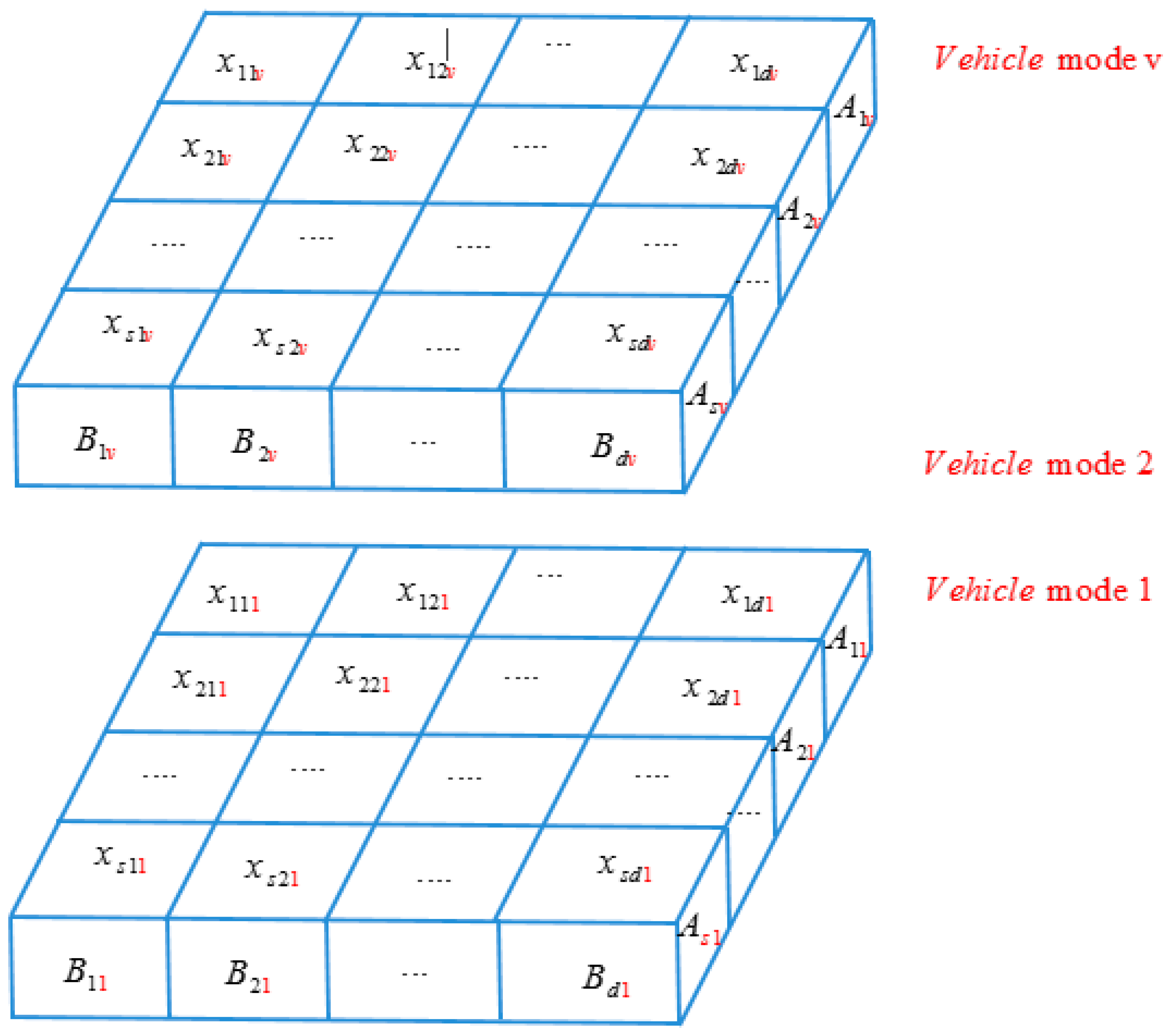
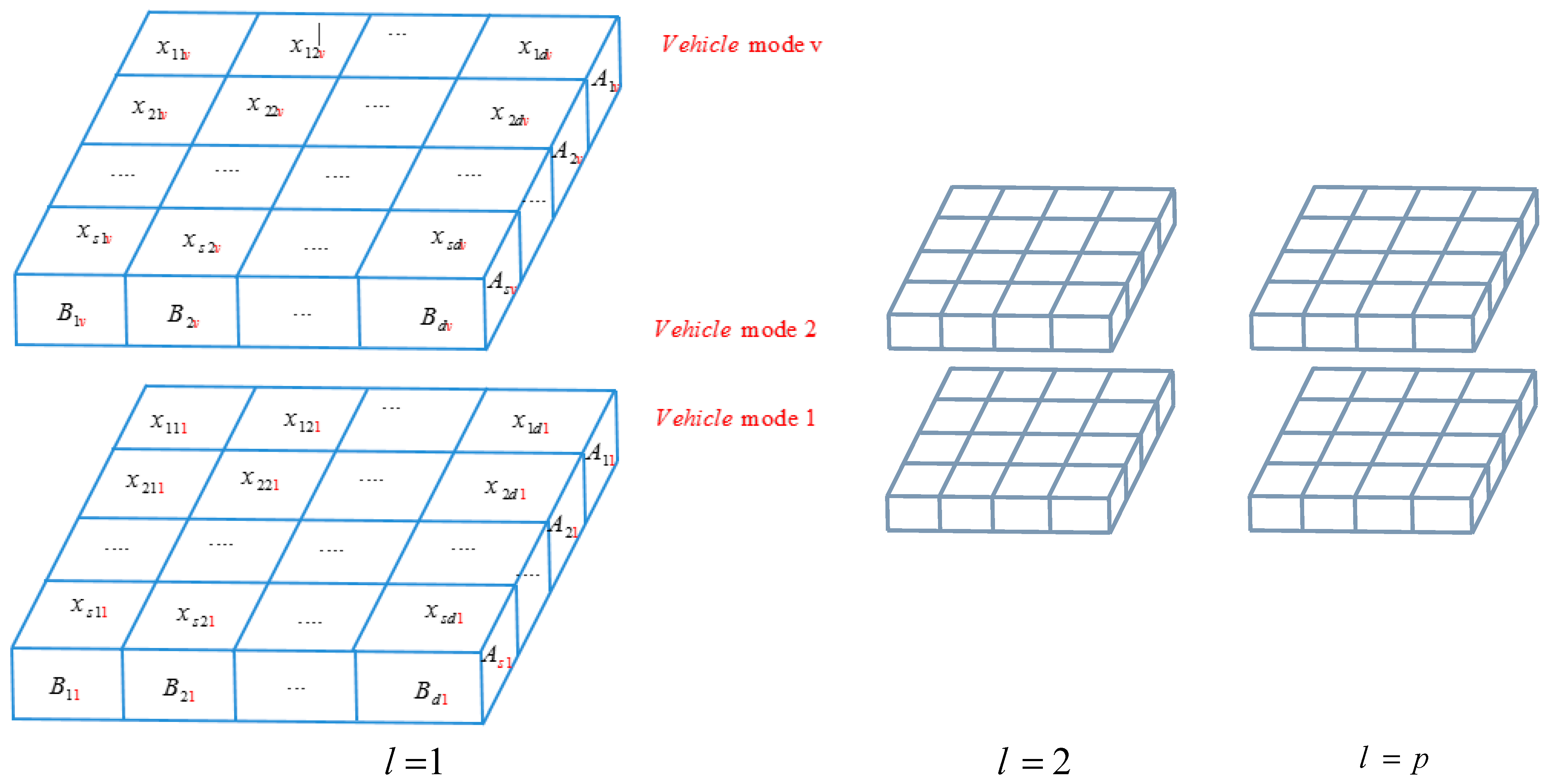
An extension of the transportation type of problem was stated by Haley [25], and may be thought of as a block in which the layers in all directions form a restricted transportation problem. The multi-index problem can be described as minimizing the cost and time of moving a set of p different commodities (l = 1, 2, …, p) from S origins (I = 1, 2, …, s) to d destinations (j = 1, 2, …, d).

The three-dimensional multi-index transportation problem can be visualized as a block of sdp cells for i = 1, 2, …, s; j = 1, 2, …, d; k = 1, 2, …, v. Each cell of this block represents one of the ${x_{ijl}}^{\prime }s$. When summed along the rows (for constant j and k) they equal $A_{jl}$. When summed along the columns (for constant l and i) they equal $B_{li}$. The arrangement of ${x_{ijl}}^{\prime }s$ and the boundary conditions are shown in Figure 1. According to the previous notations, the formulation of three index transportation can be stated as follows:

$$\begin{array}{l}3ITP:\\ Min\hspace{1em}z={\displaystyle \sum _{i=1}^s{\displaystyle \sum _{j=1}^d{\displaystyle \sum _{k=1}^v{c}_{\hspace{0.17em}i\hspace{0.17em}j\hspace{0.17em}k}^{}\hspace{0.17em}{x}_{\hspace{0.17em}i\hspace{0.17em}j\hspace{0.17em}k}}}},\\ subject\hspace{0.17em}to\\ {\displaystyle \sum _{j=1}^d{x}_{\hspace{0.17em}i\hspace{0.17em}j\hspace{0.17em}k}}=A_{\hspace{0.17em}i\hspace{0.17em}k},\hspace{0.17em}\hspace{1em}\hspace{1em}i=1,2,\dots ,s,\hspace{1em}k=1,2,\dots ,v,\\ {\displaystyle \sum _{i=1}^s{x}_{\hspace{0.17em}i\hspace{0.17em}j\hspace{0.17em}k}}=B_{\hspace{0.17em}j\hspace{0.17em}k},\hspace{0.17em}\hspace{1em}\hspace{1em}j=1,2,\dots ,d,\hspace{1em}k=1,2,\dots ,v,\\ x_{\hspace{0.17em}i\hspace{0.17em}j\hspace{0.17em}k}\ge 0,\hspace{0.17em}\hspace{1em}\hspace{1em}\forall \hspace{0.17em}i,\hspace{0.17em}j,\hspace{0.17em}k,\\ {\displaystyle \sum _{i=1}^s{A}_{\hspace{0.17em}i\hspace{0.17em}k}}={\displaystyle \sum _{j=1}^d{B}_{\hspace{0.17em}j\hspace{0.17em}k}},\hspace{0.17em}\hspace{1em}\hspace{1em}k=1,2,\dots ,v,\end{array}$$

(1)

2.2. Mathematical Formulation of the Four-Indextransportation Problem

The mathematical formulations of four-index transportation problem are presented according to earlier description. For illustrating, different notions will be used and defined as follows:

• $i,\hspace{0.17em}\hspace{0.17em}i=1,\hspace{0.17em}2,\hspace{0.17em}\dots ,\hspace{0.17em}s$ are s sources which represent the production sites.
• $j,\hspace{0.17em}\hspace{0.17em}j=1,\hspace{0.17em}2,\hspace{0.17em}\dots ,\hspace{0.17em}d$ are d destinations which represent the warehouses where the product types are transported.
• $k,\hspace{0.17em}\hspace{0.17em}k=1,\hspace{0.17em}2,\hspace{0.17em}\dots ,\hspace{0.17em}v$ represent the vehicle types or the means of transporting the product from sources to the required destinations.
• $l,\hspace{0.17em}\hspace{0.17em}l=1,\hspace{0.17em}2,\hspace{0.17em}\dots ,\hspace{0.17em}p$ represent the product types.
• $A_{\hspace{0.17em}i\hspace{0.17em}k\hspace{0.17em}l}$ represents the quantity of goods that can be transported from the source $i$ by vehicle type $k$ of product type $l$.
• $B_{\hspace{0.17em}j\hspace{0.17em}k\hspace{0.17em}l}$ represents the ordered quantity to be transported to destination $j$ by vehicle type $k$ of product type $l$.
• $c_{\hspace{0.17em}i\hspace{0.17em}j\hspace{0.17em}k\hspace{0.17em}l}$ represents the average unit cost for transporting a unit from source $i$ to destination $j$ by vehicle type $k$ of product type $l$. This unit cost will be calculated to cover the fixed and variable costs such as the distance between the sources and destinations, transit fees, and amortization costs of vehicles.
• $x_{\hspace{0.17em}i\hspace{0.17em}j\hspace{0.17em}k\hspace{0.17em}l}$ represents the quantity of goods in units transported from source $i$ to destination $j$ by vehicle type $k$ of product type $l$.

Figure 2 declares the structure of Transportation network for four-index transportation problem with m sources, n destinations, v vehicles, and p commodities.

According to the previous notations, the objective function of minimizing total cost of transportation can be defined as follows:

$$Min\hspace{1em}z={\displaystyle \sum _{i=1}^s{\displaystyle \sum _{j=1}^d{\displaystyle \sum _{k=1}^v{\displaystyle \sum _{l=1}^p{c}_{\hspace{0.17em}i\hspace{0.17em}j\hspace{0.17em}k\hspace{0.17em}l}^{}\hspace{0.17em}{x}_{\hspace{0.17em}i\hspace{0.17em}j\hspace{0.17em}k\hspace{0.17em}l}}}}}$$

(2)

Depending on the real economical requirements, agreements, and contracts, the variable can be constrained differently. According to the previous description, the constraints are defined as follows [10]:

$${\displaystyle \sum _{j=1}^d{x}_{\hspace{0.17em}i\hspace{0.17em}j\hspace{0.17em}k\hspace{0.17em}l}}=A_{\hspace{0.17em}i\hspace{0.17em}k\hspace{0.17em}l},\hspace{0.17em}\hspace{1em}\hspace{1em}i=1,2,\dots ,s,\hspace{1em}k=1,2,\dots ,v,\hspace{1em}l=1,2,\dots ,p$$

(3)

$${\displaystyle \sum _{i=1}^s{x}_{\hspace{0.17em}i\hspace{0.17em}j\hspace{0.17em}k\hspace{0.17em}l}}=B_{\hspace{0.17em}j\hspace{0.17em}k\hspace{0.17em}l},\hspace{0.17em}\hspace{1em}\hspace{1em}j=1,2,\dots ,d,\hspace{1em}k=1,2,\dots ,v,\hspace{1em}l=1,2,\dots ,p$$

(4)

$$x_{\hspace{0.17em}i\hspace{0.17em}j\hspace{0.17em}k\hspace{0.17em}l}\ge 0,\hspace{0.17em}\hspace{1em}\forall \hspace{0.17em}i,\hspace{0.17em}j,\hspace{0.17em}k,\hspace{0.17em}l$$

(5)

The first set of constraints (3) restricts the total quantities that can be transported from a source $i$ to all destinations by vehicle type $k$ of product type $l$ equal to the available quantity at source $i$ that can be transported by vehicle type $k$ of product type $l$. The second set of constraints (4) restricts the total quantities that can be transported from all sources to destination $j$ that can be transported by vehicle type $k$ of product type $l$ equal to the ordered quantity from destination $j$ to be transported by vehicle type $k$ of product type $l$. Finally, the set of constraints (5) restricts the variables to a non-negative value. See [10,11,25].

Moreover, balanced conditions must be considered, since a balanced transportation problem is a feasible problem. Balanced conditions guarantee that for each product type $l$ can be transported by vehicle type $k$, the quantities transported from all sources are equal to the quantities transported to all destinations. Therefore, balanced conditions can be defined as follows:

$${\displaystyle \sum _{i=1}^s{A}_{\hspace{0.17em}i\hspace{0.17em}k\hspace{0.17em}l}}={\displaystyle \sum _{j=1}^d{B}_{\hspace{0.17em}j\hspace{0.17em}k\hspace{0.17em}l}},\hspace{0.17em}\hspace{1em}\hspace{1em}\hspace{1em}k=1,2,\dots ,v,\hspace{1em}l=1,2,\dots ,p$$

(6)

According to the previous description, the mathematical formulation of the balanced four-index transportation problem can be defined as follows:

$$\begin{array}{l}4ITP:\\ Min\hspace{1em}z={\displaystyle \sum _{i=1}^s{\displaystyle \sum _{j=1}^d{\displaystyle \sum _{k=1}^v{\displaystyle \sum _{l=1}^p{c}_{\hspace{0.17em}i\hspace{0.17em}j\hspace{0.17em}k\hspace{0.17em}l}^{}\hspace{0.17em}{x}_{\hspace{0.17em}i\hspace{0.17em}j\hspace{0.17em}k\hspace{0.17em}l}}}}},\\ subject\hspace{0.17em}to\\ {\displaystyle \sum _{j=1}^d{x}_{\hspace{0.17em}i\hspace{0.17em}j\hspace{0.17em}k\hspace{0.17em}l}}=A_{\hspace{0.17em}i\hspace{0.17em}k\hspace{0.17em}l},\hspace{0.17em}\hspace{1em}\hspace{1em}i=1,2,\dots ,s,\hspace{1em}k=1,2,\dots ,v,\hspace{1em}l=1,2,\dots ,p,\\ {\displaystyle \sum _{i=1}^s{x}_{\hspace{0.17em}i\hspace{0.17em}j\hspace{0.17em}k\hspace{0.17em}l}}=B_{\hspace{0.17em}j\hspace{0.17em}k\hspace{0.17em}l},\hspace{0.17em}\hspace{1em}\hspace{1em}j=1,2,\dots ,d,\hspace{1em}k=1,2,\dots ,v,\hspace{1em}l=1,2,\dots ,p,\\ x_{\hspace{0.17em}i\hspace{0.17em}j\hspace{0.17em}k\hspace{0.17em}l}\ge 0,\hspace{0.17em}\hspace{1em}\forall \hspace{0.17em}i,\hspace{0.17em}j,\hspace{0.17em}k,\hspace{0.17em}l\\ {\displaystyle \sum _{i=1}^s{A}_{\hspace{0.17em}i\hspace{0.17em}k\hspace{0.17em}l}}={\displaystyle \sum _{j=1}^d{B}_{\hspace{0.17em}j\hspace{0.17em}k\hspace{0.17em}l}},\hspace{0.17em}\hspace{1em}\hspace{1em}\hspace{1em}k=1,2,\dots ,v,\hspace{1em}l=1,2,\dots ,p,\end{array}$$

(7)

2.3. Multi-Objective Four-Index Transportation Problem

In this section, we present the mathematical formulation of the multi-objective four-index transportation problem (M4ITP) that has $H,(H\ge 2)$ objectives and four indices, which can be formulated as follows:

$$\begin{array}{l}M4ITP:\\ Min\hspace{1em}{z}^h={\displaystyle \sum _{i=1}^s{\displaystyle \sum _{j=1}^d{\displaystyle \sum _{k=1}^v{\displaystyle \sum _{l=1}^p{c}_{\hspace{0.17em}i\hspace{0.17em}j\hspace{0.17em}l\hspace{0.17em}k}^h\hspace{0.17em}{x}_{\hspace{0.17em}i\hspace{0.17em}j\hspace{0.17em}k\hspace{0.17em}l}}}}},\hspace{1em}\hspace{1em}\hspace{1em}\hspace{1em}h=1,2,\dots ,H,\\ subject\hspace{0.17em}to\\ {\displaystyle \sum _{j=1}^d{x}_{\hspace{0.17em}i\hspace{0.17em}j\hspace{0.17em}k\hspace{0.17em}l}}=A_{\hspace{0.17em}i\hspace{0.17em}k\hspace{0.17em}l},\hspace{0.17em}\hspace{1em}\hspace{1em}i=1,2,\dots ,s,\hspace{1em}k=1,2,\dots ,v,\hspace{1em}l=1,2,\dots ,p,\\ {\displaystyle \sum _{i=1}^s{x}_{\hspace{0.17em}i\hspace{0.17em}j\hspace{0.17em}k\hspace{0.17em}l}}=B_{\hspace{0.17em}j\hspace{0.17em}k\hspace{0.17em}l},\hspace{0.17em}\hspace{1em}\hspace{1em}j=1,2,\dots ,d,\hspace{1em}k=1,2,\dots ,v,\hspace{1em}l=1,2,\dots ,p,\\ x_{\hspace{0.17em}i\hspace{0.17em}j\hspace{0.17em}k\hspace{0.17em}l}\ge 0,\hspace{0.17em}\hspace{1em}\forall \hspace{0.17em}i,\hspace{0.17em}j,\hspace{0.17em}k,\hspace{0.17em}l\\ {\displaystyle \sum _{i=1}^s{A}_{\hspace{0.17em}i\hspace{0.17em}k\hspace{0.17em}l}}={\displaystyle \sum _{j=1}^d{B}_{\hspace{0.17em}j\hspace{0.17em}k\hspace{0.17em}l}},\hspace{0.17em}\hspace{1em}\hspace{1em}\hspace{1em}k=1,2,\dots ,v,\hspace{1em}l=1,2,\dots ,p\end{array}$$

(8)

3. Theoretical Preliminaries

Since M4ITP is a multi-objective programming problem, the concept of optimality is exchanged with the concept of efficiency or nondominated solutions [26]. Therefore, in general M4ITP has a set of efficient solutions called the Pareto set or the set of all efficient solutions.

Definition 1. 

The index space (IS) of problem M4ITP can be defined as follows:

$$I{S}_{i\hspace{0.17em}j\hspace{0.17em}k\hspace{0.17em}l}=\left\{\left(i,\hspace{0.17em}j,\hspace{0.17em}l,\hspace{0.17em}k\right)|\hspace{0.17em}i=1,2,\dots ,s,\hspace{1em}j=1,2,\dots ,d,\hspace{1em}l=1,2,\dots ,p,\hspace{1em}k=1,2,\dots ,v\right\}$$

(9)

Definition 2. 

A feasible solution$x^{*}\in X$, where$X$represents the feasible domain of M4ITP, is an efficient solution for problem M4ITP if there is no other feasible solution$x\in X$satisfying both:

(1)

$z^h\left(x\right)\le z^h\left(x^{*}\right),\hspace{1em}h=1,2,\dots ,H$

(2)

$z^h\left(x\right)<z^h\left(x^{*}\right)$, for some $h\in \left\{1,2,\dots ,H\right\}$

Relative to M4ITP, the weighted-sum problem W4ITP can be defined as follows:

$$\begin{array}{l}W4ITP:\\ Min\hspace{1em}z={\displaystyle \sum _{h=1}^H{\displaystyle \sum _{i=1}^s{\displaystyle \sum _{j=1}^d{\displaystyle \sum _{k=1}^v{\displaystyle \sum _{l=1}^p{w}_h\hspace{0.17em}{c}_{\hspace{0.17em}i\hspace{0.17em}j\hspace{0.17em}k\hspace{0.17em}l}^h\hspace{0.17em}{x}_{\hspace{0.17em}i\hspace{0.17em}j\hspace{0.17em}k\hspace{0.17em}l}}}}}},\\ subject\hspace{0.17em}to\\ {\displaystyle \sum _{j=1}^d{x}_{\hspace{0.17em}i\hspace{0.17em}j\hspace{0.17em}k\hspace{0.17em}l}}=A_{\hspace{0.17em}i\hspace{0.17em}k\hspace{0.17em}l},\hspace{0.17em}\hspace{1em}\hspace{1em}i=1,2,\dots ,s,\hspace{1em}k=1,2,\dots ,v,\hspace{1em}l=1,2,\dots ,p,\\ {\displaystyle \sum _{i=1}^s{x}_{\hspace{0.17em}i\hspace{0.17em}j\hspace{0.17em}k\hspace{0.17em}l}}=B_{\hspace{0.17em}j\hspace{0.17em}k\hspace{0.17em}l},\hspace{0.17em}\hspace{1em}\hspace{1em}j=1,2,\dots ,d,\hspace{1em}k=1,2,\dots ,v,\hspace{1em}l=1,2,\dots ,p,\\ x_{\hspace{0.17em}i\hspace{0.17em}j\hspace{0.17em}k\hspace{0.17em}l}\ge 0,\hspace{0.17em}\hspace{1em}\hspace{1em}\forall \hspace{0.17em}i,\hspace{0.17em}j,\hspace{0.17em}l,\hspace{0.17em}k\\ {\displaystyle \sum _{i=1}^s{A}_{\hspace{0.17em}i\hspace{0.17em}k\hspace{0.17em}l}}={\displaystyle \sum _{j=1}^d{B}_{\hspace{0.17em}j\hspace{0.17em}k\hspace{0.17em}l}},\hspace{0.17em}\hspace{1em}\hspace{1em}\hspace{1em}k=1,2,\dots ,v,\hspace{1em}l=1,2,\dots ,p,\\ {\displaystyle \sum _{h\hspace{0.17em}=\hspace{0.17em}1}^H{w}_{\hspace{0.17em}h}}=1,\hspace{1em}\hspace{1em}{w}_{\hspace{0.17em}h}\ge 0,\hspace{0.17em}\hspace{1em}\forall \hspace{0.17em}h\end{array}$$

(10)

Theorem 1 

[26]. If $\overline{x}\in X$ is an optimal solution of the weighted-sum problem W4ITP where either w > 0, or $\overline{x}$ is a unique optimal solution, then $\overline{x}$ is considered a Pareto optimal solution of the M4ITP.

Theorem 2 

[26]. If $\overline{x}\in X$ is a Pareto optimal solution of the M4ITP, then $\overline{x}$ is an optimal solution of the W4ITP for some $w=(w_1,w_2,\dots ,w_k)\ge 0$.

This theorem requires convexity assumption which was guaranteed in transportation problems and hence cannot be applied for nonconvex problems. The weighting method [26] was implemented to transform multi-objective optimization to single objective optimization, due to the convexity of M4ITP. The weighting method is considered an efficient and robust method for generating all efficient solutions for convex problem. Therefore, by implementing the weighting method, we get a single objective problem W4ITP. We get different Pareto optimal solutions for the original problem M4ITP; when solving W4ITP for different weights ${\displaystyle \sum _{h\hspace{0.17em}=\hspace{0.17em}1}^H{w}_{\hspace{0.17em}h}}=1,\hspace{0.17em}\hspace{0.17em}{w}_{\hspace{0.17em}h}\ge 0,\hspace{0.17em}\hspace{0.17em}\forall \hspace{0.17em}h$, then the problem W4ITP could be considered a parametric problem in $w_h$.

Definition 3. 

The parametric space of problem W4ITP can be defined as follows:

$$W=\left\{w\in R^{\hspace{0.17em}h}|\hspace{0.17em}{\displaystyle \sum _{h\hspace{0.17em}=\hspace{0.17em}1}^H{w}_{\hspace{0.17em}h}}=1,\hspace{1em}{w}_{\hspace{0.17em}h}\ge 0,\hspace{0.17em}\hspace{0.17em}\forall \hspace{0.17em}h\right\}$$

(11)

Due to the linearity of the M4ITP, all nondominated solutions of M4ITP can be obtained by solving the W4ITP for all possible weights. Obviously, solving the W4ITP for all possible weights (${\displaystyle \sum _{h\hspace{0.17em}=\hspace{0.17em}1}^H{w}_{\hspace{0.17em}h}}=1,\hspace{1em}{w}_{\hspace{0.17em}h}\ge 0,\hspace{0.17em}\hspace{0.17em}\forall \hspace{0.17em}h$) by assigning different values is an impossible process, because there are infinite different values of weights. Therefore, it is proposed to use the Kuhn-Tucker conditions to identify the range of the weights value that retain a certain solution to be an efficient one in this range, which will be defined as the stability sets of the first kind.

In general, the W4ITP is a four-index transportation problem that has (s × d × p × v) decision variables. In addition, per Equations (2) and (3), it has ((s + d) × p × v) constraints. Obviously, it is hard to be solved by the techniques of the classical transportation problem using the curse of multi-index dimensionality. In other words, the W4ITP is characterized as:

• Large-scale problem with respect to multi-index, not efficiently solvable with respect to time and effort.
• Impossible to be solved for all possible weights.

Therefore, we propose a decomposition approach, which developed by decomposing the W4ITP into sub-problems, such that each sub-problem is a two-index transportation problem that can be handled easily by any suitable traditional technique. In addition, by implementing a parametric study for each sub-problem using the concept of the stability set of first kind, we can get all efficient solution sets of the original problem. The proposed approach saves time and effort for handling both M4ITP and W4ITP by reducing the dimension of the original problem. It also saves time to solve W4ITP for all possible weights.

Definition 4. 

The sub-problem can be defined as${\mathrm{W}4\mathrm{ITP}}_{kl},\hspace{1em}k=1,2,\dots ,v,\hspace{1em}l=1,2,\dots ,p$.

Definition 5. 

The index space of the sub-problems${\mathrm{W}4\mathrm{ITP}}_{kl},\hspace{1em}k=1,2,\dots ,v,\hspace{1em}l=1,2,\dots ,p$can be defined as follows:

$$I{S}_{\hspace{0.17em}ij}=\left\{\left(i,\hspace{0.17em}j\right)|\hspace{0.17em}i=1,2,\dots ,s;j=1,2,\dots ,d\right\}$$

(12)

The W4ITP [27] can be decomposed into (v × p) sub-problems ${\mathrm{W}4\mathrm{ITP}}_{kl}, k=1,2,\dots ,v, l=1,2,\dots ,p$. Each sub-problem is a two-index transportation problem with a dimension of (s × d) where the sub-problem can be defined as follows:

$$\begin{array}{l}W4IT{P}_{\hspace{0.17em}k\hspace{0.17em}l}:\hspace{1em}\hspace{1em}k=1,2,\dots ,v,\hspace{1em}l=1,2,\dots ,p,\\ Min\hspace{1em}z={\displaystyle \sum _{h=1}^H{\displaystyle \sum _{i=1}^s{\displaystyle \sum _{j=1}^d{w}_h\hspace{0.17em}{c}_{\hspace{0.17em}i\hspace{0.17em}j\hspace{0.17em}k\hspace{0.17em}l}^h\hspace{0.17em}{x}_{\hspace{0.17em}i\hspace{0.17em}j\hspace{0.17em}k\hspace{0.17em}l}}}},\\ subject\hspace{0.17em}to\\ {\displaystyle \sum _{j=1}^d{x}_{\hspace{0.17em}i\hspace{0.17em}j\hspace{0.17em}k\hspace{0.17em}l}}=A_{\hspace{0.17em}i\hspace{0.17em}k\hspace{0.17em}l},\hspace{0.17em}\hspace{1em}\hspace{1em}i=1,2,\dots ,s,\\ {\displaystyle \sum _{i=1}^s{x}_{\hspace{0.17em}i\hspace{0.17em}j\hspace{0.17em}k\hspace{0.17em}l}}=B_{\hspace{0.17em}j\hspace{0.17em}k\hspace{0.17em}l},\hspace{0.17em}\hspace{1em}\hspace{1em}j=1,2,\dots ,d,\\ x_{\hspace{0.17em}i\hspace{0.17em}j\hspace{0.17em}k\hspace{0.17em}l}\ge 0,\hspace{0.17em}\hspace{1em}\hspace{1em}\forall \hspace{0.17em}i,\hspace{0.17em}j,\hspace{0.17em}l,\hspace{0.17em}k\\ {\displaystyle \sum _{i=1}^s{A}_{\hspace{0.17em}i\hspace{0.17em}k\hspace{0.17em}l}}={\displaystyle \sum _{j=1}^d{B}_{\hspace{0.17em}j\hspace{0.17em}k\hspace{0.17em}l}},\hspace{0.17em}\\ {\displaystyle \sum _{h\hspace{0.17em}=\hspace{0.17em}1}^H{w}_{\hspace{0.17em}h}}=1,\hspace{1em}\hspace{1em}{w}_{\hspace{0.17em}h}\ge 0,\hspace{0.17em}\hspace{1em}\forall \hspace{0.17em}h\end{array}$$

(13)

Each sub-problem is a two-index classical transportation problem that has (s × d) decision variables and (s + d) constraints. Therefore, each sub-problem can be solved by the classical transportation techniques.

The parametric space for any sub-problem $W4IT{P}_{kl}$ equals the parametric space of all possible weights of problem W4ITP

Definition 6. 

The optimal solution of${\mathrm{W}4\mathrm{ITP}}_{kl},\hspace{1em}k=1,2,\dots ,v,\hspace{1em}l=1,2,\dots ,p$at$w\in W$is defined as

$$\begin{array}{l}{\overline{\overline{x}}}_{\hspace{0.17em}i\hspace{0.17em}j\hspace{0.17em}1\hspace{0.17em}1}^w=\left({\overline{x}}_{\hspace{0.17em}1\hspace{0.17em}1\hspace{0.17em}1\hspace{0.17em}1}^w,{\overline{x}}_{\hspace{0.17em}1\hspace{0.17em}2\hspace{0.17em}1\hspace{0.17em}1}^w,\dots ,{\overline{x}}_{\hspace{0.17em}i\hspace{0.17em}j\hspace{0.17em}1\hspace{0.17em}1}^w\right),\hspace{1em}\left(k,l\right)=\left(1,1\right),\hspace{1em}i=1,2,\dots ,s,\hspace{1em}j=1,2,\dots ,d\\ {\overline{\overline{x}}}_{\hspace{0.17em}i\hspace{0.17em}j\hspace{0.17em}1\hspace{0.17em}2}^w=\left({\overline{x}}_{\hspace{0.17em}1\hspace{0.17em}1\hspace{0.17em}1\hspace{0.17em}2}^w,{\overline{x}}_{\hspace{0.17em}1\hspace{0.17em}2\hspace{0.17em}1\hspace{0.17em}2}^w,\dots ,{\overline{x}}_{\hspace{0.17em}i\hspace{0.17em}j\hspace{0.17em}1\hspace{0.17em}2}^w\right),\hspace{1em}\left(k,l\right)=\left(1,2\right),\hspace{1em}i=1,2,\dots ,s,\hspace{1em}j=1,2,\dots ,d\\ ⋮\\ {\overline{\overline{x}}}_{\hspace{0.17em}i\hspace{0.17em}j\hspace{0.17em}v\hspace{0.17em}p}^w=\left({\overline{x}}_{\hspace{0.17em}1\hspace{0.17em}1\hspace{0.17em}v\hspace{0.17em}p}^w,{\overline{x}}_{\hspace{0.17em}1\hspace{0.17em}2\hspace{0.17em}v\hspace{0.17em}p}^w,\dots ,{\overline{x}}_{\hspace{0.17em}i\hspace{0.17em}j\hspace{0.17em}\hspace{0.17em}v\hspace{0.17em}p}^w\right),\hspace{1em}\left(k,l\right)=\left(v,p\right),\hspace{1em}i=1,2,\dots ,s,\hspace{1em}j=1,2,\dots ,d\end{array}$$

(14)

Definition 7. 

The optimal solution of the problem W4ITP at$w\in W$will be defined as:

$${\overline{x}}^w=\left({\overline{\overline{x}}}_{\hspace{0.17em}i\hspace{0.17em}j\hspace{0.17em}1\hspace{0.17em}1}^w,{\overline{\overline{x}}}_{\hspace{0.17em}i\hspace{0.17em}j\hspace{0.17em}1\hspace{0.17em}2}^w,\dots ,{\overline{\overline{x}}}_{\hspace{0.17em}i\hspace{0.17em}j\hspace{0.17em}v\hspace{0.17em}p}^w\right),\hspace{1em}i=1,2,\dots ,s,\hspace{1em}j=1,2,\dots ,d$$

(15)

where each component will be called sub-optimal at $w\in W$, where it is the optimal of a sub-problem ${\mathrm{W}4\mathrm{ITP}}_{kl},$ $k=1,2,\dots ,v,\hspace{1em}l=1,2,\dots ,p$.

Definition 8. 

The stability set of the first kind at${\overline{\overline{x}}}_{\hspace{0.17em}i\hspace{0.17em}j\hspace{0.17em}k\hspace{0.17em}l}^{\hspace{0.17em}w}$can be defined as follows:

$$S\left({\overline{\overline{x}}}_{\hspace{0.17em}i\hspace{0.17em}j\hspace{0.17em}k\hspace{0.17em}l}^{\hspace{0.17em}w}\right)=\left\{w\in W|\hspace{0.17em}{\overline{\overline{x}}}_{\hspace{0.17em}i\hspace{0.17em}j\hspace{0.17em}k\hspace{0.17em}l}^{\hspace{0.17em}w} \mathrm{is} \mathrm{the} \mathrm{optimal} \mathrm{solution} \mathrm{of} W4IT{P}_{kl}\right\}$$

(16)

The stability set of the first kind of the optimal solution ${\overline{\overline{x}}}_{\hspace{0.17em}i\hspace{0.17em}j\hspace{0.17em}k\hspace{0.17em}l}^{\hspace{0.17em}w}$ of $W4IT{P}_{k\hspace{0.17em}l},\hspace{0.17em}\left(k,l\right)\in I{S}_{\hspace{0.17em}k\hspace{0.17em}l}$ at $w\in W$ is the set of parameters that belong to the parametric space that retain the optimal solution as the optimal one.

Definition 9. 

The stability set of the first kind of the efficient solution of the problem M4ITP at$w\in W$can be defined as

$$SS\left({\overline{x}}^{\hspace{0.17em}w}\right)=\left\{w\in W|\hspace{0.17em}{\overline{x}}^{\hspace{0.17em}w} \mathrm{is} \mathrm{an} \mathrm{optimal} \mathrm{solution} \mathrm{of} \mathrm{problem} \mathrm{M}4\mathrm{ITP}\right\}$$

(17)

The stability set of the first kind of the optimal solution of the problem W4ITP at $w\in W$ is equal to $SS\left({\overline{x}}^{\hspace{0.17em}w}\right)$. Therefore, $SS\left({\overline{x}}^{\hspace{0.17em}w}\right)$ can be determined by determining the stability set of the first kind at ${\overline{\overline{x}}}_{\hspace{0.17em}i\hspace{0.17em}j\hspace{0.17em}k\hspace{0.17em}l}^{\hspace{0.17em}w},\hspace{1em}k=1,2,\dots ,v,\hspace{1em}l=1,2,\dots ,p$. In other words, $SS\left({\overline{x}}^{\hspace{0.17em}w}\right)$ is the weight that retains ${\overline{\overline{x}}}_{\hspace{0.17em}i\hspace{0.17em}j\hspace{0.17em}k\hspace{0.17em}l}^{\hspace{0.17em}w},\hspace{1em}i=1,2,\dots ,s,\hspace{1em}j=1,2,\dots ,d$ optimal solution of ${\mathrm{W}4\mathrm{ITP}}_{\mathrm{kl}},\hspace{1em}\left(k,l\right)\in I{S}_{\hspace{0.17em}kl}$.

Lemma 1. 

All the optimal solutions${\overline{\overline{x}}}_{\hspace{0.17em}w}^{\hspace{0.17em}i\hspace{0.17em}j\hspace{0.17em}k\hspace{0.17em}l}$of$W4IT{P}_{kl}$at$w\in W$represent an efficient solution for the problem M4ITP.

Proof. 

Since all optimal solutions ${\overline{\overline{x}}}_{\hspace{0.17em}i\hspace{0.17em}j\hspace{0.17em}k\hspace{0.17em}l}^{\hspace{0.17em}w}$ of ${\mathrm{W}4\mathrm{ITP}}_{kl}$ at $w\in W$ represent all sub-optimal components of the optimal solution of W4ITP at the same $w\in W$, then all optimal solutions ${\overline{\overline{x}}}_{\hspace{0.17em}i\hspace{0.17em}j\hspace{0.17em}k\hspace{0.17em}l}^{\hspace{0.17em}w}$ of ${\mathrm{W}4\mathrm{ITP}}_{kl}$ at $w\in W$ represent an efficient solution for W4ITP. □

The Lagrange function [26] for problem ${\mathrm{W}4\mathrm{ITP}}_{\mathrm{kl}},\hspace{1em}\left(k,l\right)\in I{S}_{\hspace{0.17em}kl}$ can be defined as:

$$\begin{array}{l}L={\displaystyle \sum _{h=1}^H{\displaystyle \sum _{j=1}^d{\displaystyle \sum _{i=1}^s{w}_{\hspace{0.17em}h}\hspace{0.17em}{c}_{\hspace{0.17em}i\hspace{0.17em}j\hspace{0.17em}k\hspace{0.17em}l}^{\hspace{0.17em}h}\hspace{0.17em}{x}_{\hspace{0.17em}i\hspace{0.17em}j\hspace{0.17em}k\hspace{0.17em}l}}}}+{\displaystyle \sum _{i=1}^s{u}_{\hspace{0.17em}i\hspace{0.17em}}\left({\displaystyle \sum _{j=1}^d{x}_{\hspace{0.17em}i\hspace{0.17em}j\hspace{0.17em}k\hspace{0.17em}l}-A_{\hspace{0.17em}i\hspace{0.17em}k\hspace{0.17em}l}}\right)}\\ \hfill +{\displaystyle \sum _{j=1}^d{v}_{\hspace{0.17em}j\hspace{0.17em}}\left({\displaystyle \sum _{i=1}^s{x}_{\hspace{0.17em}i\hspace{0.17em}j\hspace{0.17em}k\hspace{0.17em}l}-B_{\hspace{0.17em}j\hspace{0.17em}k\hspace{0.17em}l}}\right)}-{\displaystyle \sum _{i=1}^s{\displaystyle \sum _{j=1}^d{\gamma }_{\hspace{0.17em}i\hspace{0.17em}j\hspace{0.17em}k\hspace{0.17em}l}\hspace{0.17em}{x}_{\hspace{0.17em}i\hspace{0.17em}j\hspace{0.17em}k\hspace{0.17em}l}}},\hfill \end{array}$$

(18)

Therefore, the Kuhn-Tucker conditions [28] for ${\mathrm{W}4\mathrm{ITP}}_{\mathrm{kl}},\hspace{1em}\left(k,l\right)\in I{S}_{\hspace{0.17em}kl}$ can be defined as:

$$\begin{array}{l}\frac{\partial L}{\partial x_{\hspace{0.17em}i\hspace{0.17em}j\hspace{0.17em}k\hspace{0.17em}l}}=0,\hspace{1em}\hspace{1em}i=1,2,\dots ,s,\hspace{0.17em}\hspace{1em}j=1,2,\dots ,d,\\ u_{\hspace{0.17em}i\hspace{0.17em}}\left({\displaystyle \sum _{d=1}^D{x}_{\hspace{0.17em}i\hspace{0.17em}j\hspace{0.17em}k\hspace{0.17em}l}-A_{\hspace{0.17em}i\hspace{0.17em}k\hspace{0.17em}l}}\right)=0,\hspace{1em}\hspace{1em}i=1,2,\dots ,s,\\ v_{\hspace{0.17em}j\hspace{0.17em}}\left({\displaystyle \sum _{s=1}^S{x}_{\hspace{0.17em}i\hspace{0.17em}j\hspace{0.17em}k\hspace{0.17em}l}-B_{\hspace{0.17em}j\hspace{0.17em}k\hspace{0.17em}l}}\right)=0,\hspace{1em}\hspace{1em}j=1,2,\dots ,d\\ {\gamma }_{\hspace{0.17em}i\hspace{0.17em}j\hspace{0.17em}k\hspace{0.17em}l}\hspace{0.17em}{x}_{\hspace{0.17em}i\hspace{0.17em}j\hspace{0.17em}k\hspace{0.17em}l}=0,\hspace{0.17em}\hspace{0.17em}\hspace{0.17em}\hspace{1em}i=1,2,\dots ,s,\hspace{1em}\hspace{0.17em}j=1,2,\dots ,d,\\ {\gamma }_{\hspace{0.17em}i\hspace{0.17em}j\hspace{0.17em}k\hspace{0.17em}l}\ge 0,\hspace{1em}\hspace{1em}i=1,2,\dots ,s,\hspace{1em}j=1,2,\dots ,d,\end{array}$$

(19)

On solving this system of equations and inequalities at the obtained optimal solution of ${\mathrm{W}4\mathrm{ITP}}_{kl}$, the range of the weights value that retain that solution is an optimal one.

4. The Proposed Algorithm

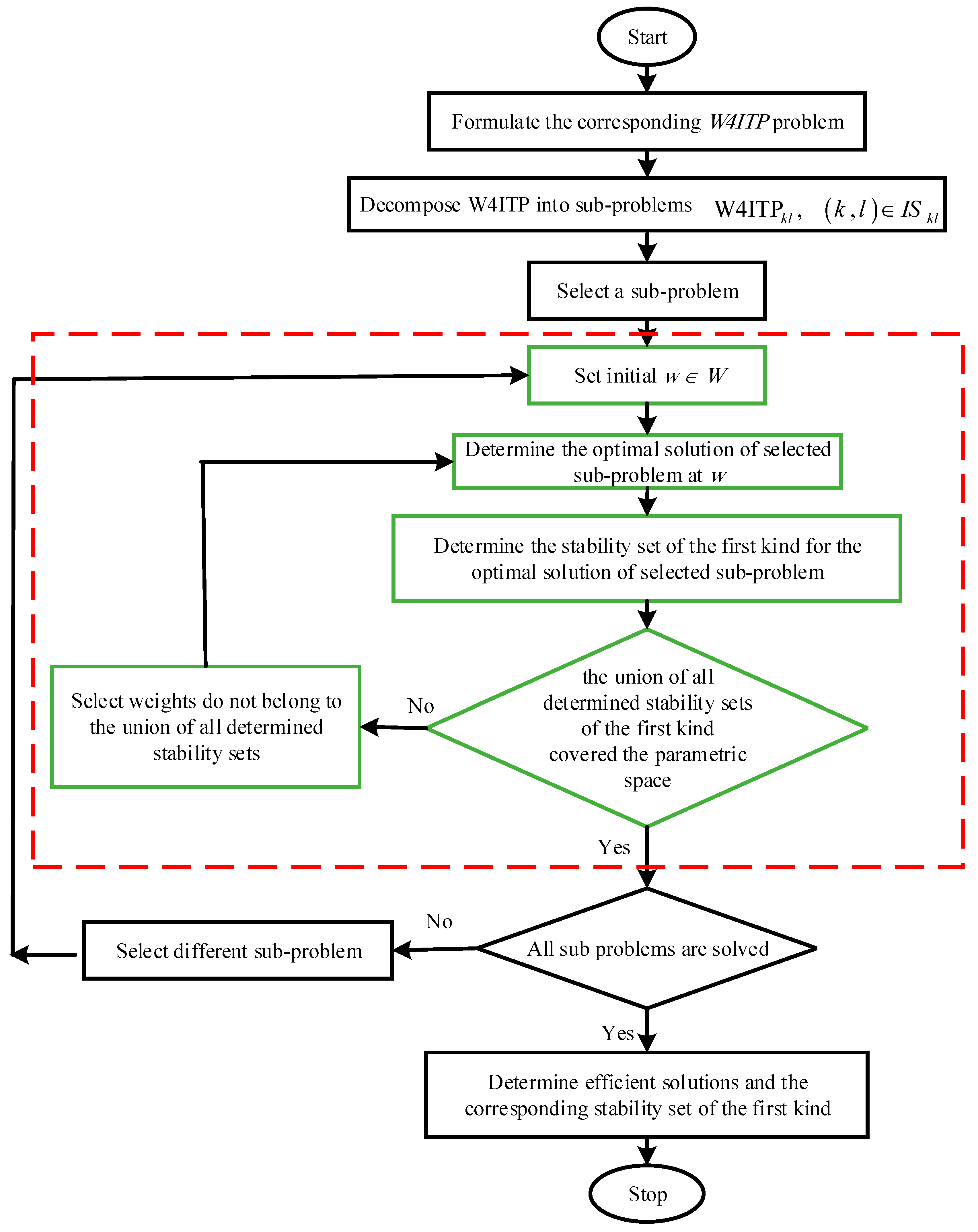
• Formulate the corresponding W4ITP problem of the M4ITP problem.
• Decompose W4ITP into $(v\times p)$ two dimensional sub-problems (${\mathrm{W}4\mathrm{ITP}}_{kl},\hspace{1em}\left(k,l\right)\in I{S}_{\hspace{0.17em}kl}$).
• Select $\left(k,l\right)\in I{S}_{\hspace{0.17em}kl}$.
• Set initial weights $w\in R^H$ (i.e., $w=\left(0,0,\dots ,0\right)$).
• Determine an optimal solution ${\overline{\overline{x}}}_{i\hspace{0.17em}j\hspace{0.17em}k\hspace{0.17em}l}^{\hspace{0.17em}w}$ for the selected problem ${\mathrm{W}4\mathrm{ITP}}_{kl},\hspace{1em}\left(k,l\right)\in I{S}_{\hspace{0.17em}kl}$ at $w$.
• Determine the stability set of the first kind $S\left({\overline{\overline{x}}}_{i\hspace{0.17em}j\hspace{0.17em}k\hspace{0.17em}l}^{\hspace{0.17em}w}\right)$ by utilizing the Kuhn-Tucker conditions.
• If the union of all determined stability sets of the first kind ${\displaystyle {\displaystyle \bigcup }_{kl}S\left({\overline{\overline{x}}}_{\hspace{0.17em}ijkl}^{\hspace{0.17em}w}\right)}$ does not cover all the parametric space then choose another $w$ that does not belong to the union of all determined stability sets of the first kind of the selected problem $\left\{w|w\notin {\displaystyle {\displaystyle \bigcup }_{kl}S\left({\overline{\overline{x}}}_{\hspace{0.17em}ijkl}^{\hspace{0.17em}w}\right)}\right\}$ and go to step 5, otherwise to step 3 until all sub-problems (${\mathrm{W}4\mathrm{ITP}}_{kl},\hspace{1em}\left(k,l\right)\in I{S}_{\hspace{0.17em}kl}$) are solved.
• Determine each optimal solution of $\mathrm{W}4\mathrm{ITP}$ (all efficient solutions of $\mathrm{M}4\mathrm{ITP}$) and the corresponding stability set of the first kind for each obtained efficient solution.
• Stop.

Figure 3 illustrates the flow chart of the proposed algorithm.

5. An Illustrative Example

The following problem is a multi-objective four-index transportation problem that has two objectives to be minimized. In addition, the problem has two sources $\left(i=1,2\right)$ with three destinations $\left(j=1,2,3\right)$ and three types of products $\left(l=1,2,3\right)$ that can be transported by two vehicle types $\left(k=1,2\right)$. The following mathematical model represents that problem. Moreover,

Table 1. The required data of the illustrative example.

	$(\mathbf{Vehicle} \mathbf{Type}, \mathbf{Product} \mathbf{Type})=\left(\mathit{k},\hspace{0.17em}\mathit{l}\right)$
	(1, 1)	(2, 1)	(1, 2)	(2, 2)	(1, 3)	(2, 3)
$\left(c^1{}_{1\hspace{0.17em}1\hspace{0.17em}k\hspace{0.17em}l},c^2{}_{1\hspace{0.17em}1\hspace{0.17em}k\hspace{0.17em}l}\right)$	(150, 200)	(800, 600)	(250, 700)	(500, 350)	(600, 800)	(1200, 1000)
$\left(c^1{}_{1\hspace{0.17em}2\hspace{0.17em}k\hspace{0.17em}l},c^2{}_{1\hspace{0.17em}2\hspace{0.17em}k\hspace{0.17em}l}\right)$	(400, 500)	(700, 750)	(450, 600)	(400, 500)	(800, 600)	(800, 1200)
$\left(c^1{}_{1\hspace{0.17em}3\hspace{0.17em}k\hspace{0.17em}l},c^2{}_{1\hspace{0.17em}3\hspace{0.17em}k\hspace{0.17em}l}\right)$	(350, 300)	(1000, 500)	(550, 900)	(600, 400)	(430, 500)	(1000, 800)
$\left(c^1{}_{2\hspace{0.17em}1\hspace{0.17em}k\hspace{0.17em}l},c^2{}_{2\hspace{0.17em}1\hspace{0.17em}k\hspace{0.17em}l}\right)$	(550, 600)	(500, 550)	(700, 600)	(800, 600)	(650, 700)	(750, 800)
$\left(c^1{}_{2\hspace{0.17em}2\hspace{0.17em}k\hspace{0.17em}l},c^2{}_{2\hspace{0.17em}2\hspace{0.17em}k\hspace{0.17em}l}\right)$	(700, 800)	(850, 600)	(800, 750)	(1000, 750)	(1000, 900)	(1100, 800)
$\left(c^1{}_{2\hspace{0.17em}3\hspace{0.17em}k\hspace{0.17em}l},c^2{}_{2\hspace{0.17em}3\hspace{0.17em}k\hspace{0.17em}l}\right)$	(300, 400)	(600, 480)	(600, 500)	(900, 400)	(850, 1100)	(850, 750)
$a_{\hspace{0.17em}1\hspace{0.17em}k\hspace{0.17em}l}$	100	175	150	300	200	250
$a_{\hspace{0.17em}2\hspace{0.17em}k\hspace{0.17em}l}$	125	400	300	300	400	100
$b_{\hspace{0.17em}1\hspace{0.17em}k\hspace{0.17em}l}$	80	175	210	225	180	140
$b_{\hspace{0.17em}2\hspace{0.17em}k\hspace{0.17em}l}$	90	350	140	250	250	110
$b_{\hspace{0.17em}3\hspace{0.17em}k\hspace{0.17em}l}$	55	50	100	125	170	100

illustrates the required data of the illustrative example.

For solving this illustrative example, we are going to apply the proposed algorithm as follows:

• Step (1):

By using the weighting method as a scalarization technique for solving a multi-objective programming problem, formulate the $\mathrm{W}4\mathrm{ITP}$ corresponding to the $\mathrm{M}4\mathrm{ITP}$ as illustrated below.

$$\begin{array}{l}W4ITP:\\ Min\hspace{1em}z={\displaystyle \sum _{i=1}^2{\displaystyle \sum _{j=1}^3{\displaystyle \sum _{k=1}^2{\displaystyle \sum _{l=1}^3\left(w\hspace{0.17em}{c}_{\hspace{0.17em}i\hspace{0.17em}j\hspace{0.17em}k\hspace{0.17em}l}^{\hspace{0.17em}1}\hspace{0.17em}{x}_{\hspace{0.17em}i\hspace{0.17em}j\hspace{0.17em}k\hspace{0.17em}l}+\left(1-w\right)c_{\hspace{0.17em}i\hspace{0.17em}j\hspace{0.17em}k\hspace{0.17em}l}^{\hspace{0.17em}2}\hspace{0.17em}{x}_{\hspace{0.17em}i\hspace{0.17em}j\hspace{0.17em}k\hspace{0.17em}l}\right)}}}},\\ subject\hspace{0.17em}to\\ {\displaystyle \sum _{j=1}^3{x}_{\hspace{0.17em}i\hspace{0.17em}j\hspace{0.17em}k\hspace{0.17em}l}}=A_{\hspace{0.17em}i\hspace{0.17em}k\hspace{0.17em}l},\hspace{0.17em}\hspace{1em}i=1,2,\hspace{0.17em}\hspace{1em}k=1,2,\hspace{0.17em}\hspace{1em}l=1,2,3,\\ {\displaystyle \sum _{i=1}^2{x}_{\hspace{0.17em}i\hspace{0.17em}j\hspace{0.17em}k\hspace{0.17em}l}}=B_{\hspace{0.17em}j\hspace{0.17em}k\hspace{0.17em}l},\hspace{0.17em}\hspace{1em}j=1,2,3,\hspace{0.17em}\hspace{1em}k=1,2,\hspace{0.17em}\hspace{1em}l=1,2,3,\\ x_{\hspace{0.17em}i\hspace{0.17em}j\hspace{0.17em}k\hspace{0.17em}l}\ge 0,\hspace{0.17em}\hspace{1em}\hspace{1em}\hspace{0.17em}\forall i,j,k,l\\ {\displaystyle \sum _{i=1}^2{A}_{\hspace{0.17em}i\hspace{0.17em}k\hspace{0.17em}l}}={\displaystyle \sum _{j=1}^3{B}_{\hspace{0.17em}j\hspace{0.17em}k\hspace{0.17em}l}},\hspace{0.17em}\hspace{1em}k=1,2,\hspace{0.17em}\hspace{1em}l=1,2,3,\end{array}$$

(20)

• Step (2):

Decompose the problem into six sub-problems $W4IT{P}_{kl}$ for all combination of $k=1,2; l=1,2,3$ as illustrated below.

$$\begin{array}{l}{\mathrm{W}4\mathrm{ITP}}_{11} \mathrm{coresponding} \mathrm{to} k=1, l=1\\ {\mathrm{W}4\mathrm{ITP}}_{21} \mathrm{coresponding} \mathrm{to} k=2, l=1\\ {\mathrm{W}4\mathrm{ITP}}_{12} \mathrm{coresponding} \mathrm{to} k=1, l=2\\ {\mathrm{W}4\mathrm{ITP}}_{22} \mathrm{coresponding} \mathrm{to} k=2, l=2\\ {\mathrm{W}4\mathrm{ITP}}_{13} \mathrm{coresponding} \mathrm{to} k=1, l=3\\ {\mathrm{W}4\mathrm{ITP}}_{23} \mathrm{coresponding} \mathrm{to} k=2, l=3\end{array}$$

Clearly, each problem $W4IT{P}_{kl}$ is linear programming that has six variables and four linearly independent equality constraints, which can be simply solved.

• Step (3):

For each sub-problem $W4IT{P}_{kl}$, find the optimal solutions corresponding to different weights that cover all parametric ranges, which can be defined as:

$$\begin{array}{ll}W& =\left\{\left(w_{\hspace{0.17em}1},w_{\hspace{0.17em}2}\right)\in R^{\hspace{0.17em}2}|\hspace{0.17em}{\displaystyle \sum _{h\hspace{0.17em}=\hspace{0.17em}1}^2{w}_{\hspace{0.17em}h}}=1,\hspace{1em}{w}_{\hspace{0.17em}h}\ge 0,\hspace{0.17em}\hspace{0.17em}\forall \hspace{0.17em}h\right\}\\ & =\left\{\left(w_{\hspace{0.17em}1},w_{\hspace{0.17em}2}\right)\in R^{\hspace{0.17em}2}|\hspace{0.17em}{w}_{\hspace{0.17em}1}=w,\hspace{0.17em}{w}_{\hspace{0.17em}2}=\left(1-w\right),\hspace{0.17em}w\in \left[0,1\right]\hspace{0.17em}\right\}\end{array}$$

(21)

For instance, suppose that the selected sub-problem is defined as $\left(k, l\right)=\left(2, l\right)\in I{S}_{k\hspace{0.17em}l}$. Therefore, the sub-problem is formulated as follows:

$$\begin{array}{l}{\mathrm{W}4\mathrm{ITP}}_{2\hspace{0.17em}1}:\\ Min\hspace{1em}z=\left\{\begin{array}{l}\left(w\hspace{0.17em}{c}_{\hspace{0.17em}1\hspace{0.17em}1\hspace{0.17em}2\hspace{0.17em}1}^{\hspace{0.17em}1}\hspace{0.17em}{x}_{\hspace{0.17em}1\hspace{0.17em}1\hspace{0.17em}2\hspace{0.17em}1}+\left(1-w\right)c_{\hspace{0.17em}1\hspace{0.17em}1\hspace{0.17em}2\hspace{0.17em}1}^{\hspace{0.17em}2}\hspace{0.17em}{x}_{\hspace{0.17em}1\hspace{0.17em}1\hspace{0.17em}2\hspace{0.17em}1}\right)+\left(w\hspace{0.17em}{c}_{\hspace{0.17em}2\hspace{0.17em}1\hspace{0.17em}2\hspace{0.17em}1}^{\hspace{0.17em}1}\hspace{0.17em}{x}_{\hspace{0.17em}2\hspace{0.17em}1\hspace{0.17em}2\hspace{0.17em}1}+\left(1-w\right)c_{\hspace{0.17em}2\hspace{0.17em}1\hspace{0.17em}2\hspace{0.17em}1}^{\hspace{0.17em}2}\hspace{0.17em}{x}_{\hspace{0.17em}2\hspace{0.17em}1\hspace{0.17em}2\hspace{0.17em}1}\right)+\\ \left(w\hspace{0.17em}{c}_{\hspace{0.17em}1\hspace{0.17em}2\hspace{0.17em}2\hspace{0.17em}1}^{\hspace{0.17em}1}\hspace{0.17em}{x}_{\hspace{0.17em}1\hspace{0.17em}2\hspace{0.17em}2\hspace{0.17em}1}+\left(1-w\right)c_{\hspace{0.17em}1\hspace{0.17em}2\hspace{0.17em}2\hspace{0.17em}1}^{\hspace{0.17em}2}\hspace{0.17em}{x}_{\hspace{0.17em}1\hspace{0.17em}2\hspace{0.17em}2\hspace{0.17em}1}\right)+\left(w\hspace{0.17em}{c}_{\hspace{0.17em}2\hspace{0.17em}2\hspace{0.17em}2\hspace{0.17em}1}^{\hspace{0.17em}1}\hspace{0.17em}{x}_{\hspace{0.17em}2\hspace{0.17em}2\hspace{0.17em}2\hspace{0.17em}1}+\left(1-w\right)c_{\hspace{0.17em}2\hspace{0.17em}2\hspace{0.17em}2\hspace{0.17em}1}^{\hspace{0.17em}2}\hspace{0.17em}{x}_{\hspace{0.17em}2\hspace{0.17em}2\hspace{0.17em}2\hspace{0.17em}1}\right)+\\ \left(w\hspace{0.17em}{c}_{\hspace{0.17em}1\hspace{0.17em}3\hspace{0.17em}2\hspace{0.17em}1}^{\hspace{0.17em}1}\hspace{0.17em}{x}_{\hspace{0.17em}1\hspace{0.17em}3\hspace{0.17em}2\hspace{0.17em}1}+\left(1-w\right)c_{\hspace{0.17em}1\hspace{0.17em}3\hspace{0.17em}2\hspace{0.17em}1}^{\hspace{0.17em}2}\hspace{0.17em}{x}_{\hspace{0.17em}1\hspace{0.17em}3\hspace{0.17em}2\hspace{0.17em}1}\right)+\left(w\hspace{0.17em}{c}_{\hspace{0.17em}2\hspace{0.17em}3\hspace{0.17em}2\hspace{0.17em}1}^{\hspace{0.17em}1}\hspace{0.17em}{x}_{\hspace{0.17em}2\hspace{0.17em}3\hspace{0.17em}2\hspace{0.17em}1}+\left(1-w\right)c_{\hspace{0.17em}2\hspace{0.17em}3\hspace{0.17em}2\hspace{0.17em}1}^{\hspace{0.17em}2}\hspace{0.17em}{x}_{\hspace{0.17em}2\hspace{0.17em}3\hspace{0.17em}2\hspace{0.17em}1}\right)\end{array}\right\},\\ subject\hspace{0.17em}to\\ x_{\hspace{0.17em}1\hspace{0.17em}1\hspace{0.17em}2\hspace{0.17em}1}+x_{\hspace{0.17em}1\hspace{0.17em}2\hspace{0.17em}2\hspace{0.17em}1}+x_{\hspace{0.17em}1\hspace{0.17em}3\hspace{0.17em}2\hspace{0.17em}1}=A_{\hspace{0.17em}1\hspace{0.17em}2\hspace{0.17em}1},\\ x_{\hspace{0.17em}2\hspace{0.17em}1\hspace{0.17em}2\hspace{0.17em}1}+x_{\hspace{0.17em}2\hspace{0.17em}2\hspace{0.17em}2\hspace{0.17em}1}+x_{\hspace{0.17em}2\hspace{0.17em}3\hspace{0.17em}2\hspace{0.17em}1}=A_{\hspace{0.17em}2\hspace{0.17em}2\hspace{0.17em}1},\\ x_{\hspace{0.17em}1\hspace{0.17em}1\hspace{0.17em}2\hspace{0.17em}1}+x_{\hspace{0.17em}2\hspace{0.17em}1\hspace{0.17em}2\hspace{0.17em}1}=B_{\hspace{0.17em}1\hspace{0.17em}2\hspace{0.17em}1},\\ x_{\hspace{0.17em}1\hspace{0.17em}2\hspace{0.17em}2\hspace{0.17em}1}+x_{\hspace{0.17em}2\hspace{0.17em}2\hspace{0.17em}2\hspace{0.17em}1}=B_{\hspace{0.17em}2\hspace{0.17em}2\hspace{0.17em}1},\\ x_{\hspace{0.17em}1\hspace{0.17em}3\hspace{0.17em}2\hspace{0.17em}1}+x_{\hspace{0.17em}2\hspace{0.17em}3\hspace{0.17em}2\hspace{0.17em}1}=B_{\hspace{0.17em}3\hspace{0.17em}2\hspace{0.17em}1},\\ x_{\hspace{0.17em}s\hspace{0.17em}d\hspace{0.17em}2\hspace{0.17em}1}\ge 0,\hspace{0.17em}\hspace{1em}s=1,2,\hspace{1em}d=1,2,3,\\ A_{\hspace{0.17em}1\hspace{0.17em}2\hspace{0.17em}1}+A_{\hspace{0.17em}2\hspace{0.17em}2\hspace{0.17em}1}=B_{\hspace{0.17em}1\hspace{0.17em}2\hspace{0.17em}1}+B_{\hspace{0.17em}2\hspace{0.17em}2\hspace{0.17em}1}+B_{\hspace{0.17em}3\hspace{0.17em}2\hspace{0.17em}1}\\ w\in \left[0,1\right]\end{array}$$

where the required data for the selected sub-problem is given by the 2nd column in Table 1.

In general, a two-index classical transportation problem has one dependent constraint that can be eliminated to get a linear programming problem in independent constraints only [1]. Since $W4IT{P}_{kl}$ is considered a classical transportation problem, one of the constraints can be eliminated to get a linear programming problem that has six variables and four constraints. Therefore, it can be reduced to a linear programming problem that has (6 − 4) = 2 variables which can be solved graphically. For simplicity, the reduced form of $W4IT{P}_{2\hspace{0.17em}1}$ will be denoted by $R_{\hspace{0.17em}2\hspace{0.17em}1}$ that can be formulated as illustrated below:

$$\begin{array}{l}{R}_{\hspace{0.17em}2\hspace{0.17em}1}:\\ Min\hspace{1em}z=\left(-130\hspace{0.17em}w+30\right)\hspace{0.17em}x+\left(-680\hspace{0.17em}w+130\right)\hspace{0.17em}y\hspace{0.17em}+\left(146750\hspace{0.17em}w+338250\right),\\ subject\hspace{0.17em}to\\ x\hspace{1em}\le 175,\\ \hspace{1em}y\le 350,\\ -x-y\le -125,\\ x+y\le 175,\\ x,\hspace{0.17em}y\ge 0\end{array}$$

where

$$\begin{array}{lll}{x}_{\hspace{0.17em}1\hspace{0.17em}1\hspace{0.17em}2\hspace{0.17em}1}=x,& x_{\hspace{0.17em}1\hspace{0.17em}2\hspace{0.17em}2\hspace{0.17em}1}=y,& x_{\hspace{0.17em}1\hspace{0.17em}3\hspace{0.17em}2\hspace{0.17em}1}=175-x-y,\\ x_{\hspace{0.17em}2\hspace{0.17em}1\hspace{0.17em}2\hspace{0.17em}1}=175-x,& x_{\hspace{0.17em}2\hspace{0.17em}2\hspace{0.17em}2\hspace{0.17em}1}=350-y,& x_{\hspace{0.17em}2\hspace{0.17em}3\hspace{0.17em}2\hspace{0.17em}1}=-125+x+y\end{array}$$

• Step (4):

Select initial $w=0\in \left[0,1\right]$

• Step (5):

Using the Lindo software package, find the optimal solution for ${\overline{\overline{x}}}_{\hspace{0.17em}i\hspace{0.17em}j\hspace{0.17em}2\hspace{0.17em}1}^{\hspace{0.17em}0}$ at $w=0$ for the problem $R_{\hspace{0.17em}2\hspace{0.17em}1}$, which is (x, y) = (125, 0)

• Step (6):

Determine the stability set of the first kind $S\left({\overline{\overline{x}}}_{\hspace{0.17em}12\hspace{0.17em}2\hspace{0.17em}1}^{\hspace{0.17em}0}\right)$ by implementing the Kuhn-Tucker conditions as follows:

$$\begin{array}{l}\left(-130\hspace{0.17em}w+30\right)+u_{\hspace{0.17em}1}-u_{\hspace{0.17em}3}+u_{\hspace{0.17em}4}-v_{\hspace{0.17em}1}=0,\\ \left(-680\hspace{0.17em}w+130\right)+u_{\hspace{0.17em}2}-u_{\hspace{0.17em}3}+u_{\hspace{0.17em}4}-v_{\hspace{0.17em}2}=0,\\ u_{\hspace{0.17em}1}\left(x-175\right)=0,\\ u_{\hspace{0.17em}2}\left(y-350\right)=0,\\ u_{\hspace{0.17em}3}\left(-x-y+125\right)=0,\\ u_{\hspace{0.17em}4}\left(x+y-175\right)=0,\\ -v_{\hspace{0.17em}1}\hspace{0.17em}x=0,\\ -v_{\hspace{0.17em}2}\hspace{0.17em}y=0,\\ x-175\le 0,\\ y-350\le 0,\\ -x-y+125\le 0,\\ x+y-175\le 0,\\ x,y,u_{\hspace{0.17em}1},u_{\hspace{0.17em}2},u_{\hspace{0.17em}3},u_{\hspace{0.17em}4},v_{\hspace{0.17em}1},v_{\hspace{0.17em}2}\ge 0\end{array}$$

By assigning (x, y) = (125, 0) and solving the resulting system, the stability set of first kind can be defined as follows:

$$S\left({\overline{\overline{x}}}_{\hspace{0.17em}i\hspace{0.17em}j\hspace{0.17em}2\hspace{0.17em}1}^{\hspace{0.17em}0}\right)=\left\{w\in \left[0,\hspace{0.17em}2/11\right)|\hspace{0.17em}\left(125,\hspace{0.17em}0\right) \mathrm{is} \mathrm{optimal} \mathrm{of} \mathrm{problem}\hspace{0.17em}{R}_{\hspace{0.17em}2\hspace{0.17em}1}\right\}$$

(22)

• Step (7):

Since all determined stability sets of the first kind do not cover the parametric space $W=\left[0,1\right]$, choose another $w\in \left(W-{\displaystyle \bigcup }S\left({\overline{\overline{x}}}_{\hspace{0.17em}s\hspace{0.17em}d\hspace{0.17em}1\hspace{0.17em}2}^{\hspace{0.17em}w}\right)\right)=\left[0,1\right]-\left[0,\hspace{0.17em}2/11\right)$ (i.e., $w=2/11$) and go to step 5 to find the optimal solution that covers all the range of parametric space.

By repeating the previous steps, the following stability sets of the first kind can be determined:

$$S\left({\overline{\overline{x}}}_{\hspace{0.17em}i\hspace{0.17em}j\hspace{0.17em}2\hspace{0.17em}1}^{\hspace{0.17em}2/11}\right)=\left\{w=2/11|\hspace{0.17em}{\overline{\overline{x}}}_{\hspace{0.17em}i\hspace{0.17em}j\hspace{0.17em}2\hspace{0.17em}1}^{\hspace{0.17em}2/11} \mathrm{is} \mathrm{optimal} \mathrm{of} \mathrm{problem}\hspace{0.17em}{R}_{\hspace{0.17em}2\hspace{0.17em}1}\right\}$$

(23)

$$S\left({\overline{\overline{x}}}_{\hspace{0.17em}i\hspace{0.17em}j\hspace{0.17em}2\hspace{0.17em}1}^{\hspace{0.17em}0.2}\right)=\left\{w\in \left(2/11,1\right]|\hspace{0.17em}{\overline{\overline{x}}}_{\hspace{0.17em}i\hspace{0.17em}j\hspace{0.17em}2\hspace{0.17em}1}^{\hspace{0.17em}0.2} \mathrm{is} \mathrm{optimal} \mathrm{of} R_{\hspace{0.17em}2\hspace{0.17em}1} \mathrm{problem}\right\}$$

(24)

where:

$${\overline{\overline{x}}}_{\hspace{0.17em}i\hspace{0.17em}j\hspace{0.17em}2\hspace{0.17em}1}^{\hspace{0.17em}2/11}=\left\{\left(x,y\right)|\hspace{0.17em}\left(x,y\right)=\lambda \left(125,0\right)+\left(1-\lambda \right)\left(0,125\right),\hspace{0.17em}0\le \lambda \le 1,\hspace{0.17em}\hspace{0.17em}x,y\hspace{0.17em}\mathrm{integers}\right\},$$

(25)

$${\overline{\overline{x}}}_{\hspace{0.17em}i\hspace{0.17em}j\hspace{0.17em}2\hspace{0.17em}1}^{\hspace{0.17em}0.2}=\left\{\left(x,y\right)|\hspace{0.17em}\left(x,y\right)=\left(0,175\right)\right\}$$

(26)

Now, when all determined stability sets of the first kind cover the parametric space, select different combination of k and l, that is, $\left(k, l\right)\in I{S}_{k\hspace{0.17em}l}-\left\{\left(2, l\right)\right\}$.

By repeating the previous steps, the following stability sets of the first kind can be determined as illustrated in

Table 2. The optimal solution $\left(\overline{x},\overline{y}\right)$ of $R_{\hspace{0.17em}lk}$ with respect to $w$.

$\left(\mathit{k},\hspace{0.17em}\mathit{l}\right)$	$\mathit{w}$	$\mathbf{Optimal} \mathbf{Solution} \left(\overline{\mathit{x}},\overline{\mathit{y}}\right)$
(1, 1)	∈[0, 1]	(80, 20)
(2, 1)	∈[0, 2/11]	(125, 0)
	=2/11	$\in \left\{\left(x,y\right)|\hspace{0.17em}\left(x,y\right)=\lambda \left(125,0\right)+\left(1-\lambda \right)\left(0,125\right),\hspace{0.17em}0\le \lambda \le 1,\hspace{0.17em}\hspace{0.17em}x,y\hspace{0.17em}\mathrm{integers}\right\}$
	∈(2/11, 1]	(0, 175)
(1, 2)	∈[0, 5/7]	(10, 140)
	=5/7	$\in \left\{\left(x,y\right)|\hspace{0.17em}\left(x,y\right)=\lambda \left(10,140\right)+\left(1-\lambda \right)\left(150,0\right),\hspace{0.17em}0\le \lambda \le 1,\hspace{0.17em}\hspace{0.17em}x,y\hspace{0.17em}\mathrm{integers}\right\}$
	∈[5/7, 1]	(150, 0)
(2, 2)	∈[0, 1]	(50, 250)
(1, 3)	∈[0, 1]	(0, 30)
(2, 3)	∈[0, 4/19]	(140, 10)
	=4/19	$\in \left\{\left(x,y\right)|\hspace{0.17em}\left(x,y\right)=\lambda \left(140,10\right)+\left(1-\lambda \right)\left(40,110\right),\hspace{0.17em}0\le \lambda \le 1,\hspace{0.17em}\hspace{0.17em}x,y\hspace{0.17em}\mathrm{integers}\right\}$
	∈[4/19, 1]	(40, 110)

and

Table 3. The optimal solution $\left(\overline{x},\overline{y}\right)$ of $R_{\hspace{0.17em}k\hspace{0.17em}l}$ with respect to $w$.

	$\mathit{w}\in$	$\left[0,2/11\right]$	$\left(2/11,4/19\right]$	$\left(4/19,5/7\right]$	$\left(5/7,1\right]$
$\left(\mathit{k},\hspace{0.17em}\mathit{l}\right)$
(1, 1)		(80, 20)	(80, 20)	(80, 20)	(80, 20)
(2, 1)		(125, 0)	(0, 175)	(0, 175)	(0, 175)
(1, 2)		(10, 140)	(10, 140)	(10, 140)	(150, 0)
(2, 2)		(50, 250)	(50, 250)	(50, 250)	(50, 250)
(1, 3)		(0, 30)	(0, 30)	(0, 30)	(0, 30)
(2, 3)		(140, 10)	(140, 10)	(40, 110)	(40, 110)

:

• Step (8):

Determine each optimal solution of W4ITP (all efficient solutions of M4ITP) and the corresponding stability set of the first kind for each obtained efficient solution. It can be noted that four different solutions were obtained for the W4ITP. Therefore, all efficient solutions of the illustrative example can be illustrated through the following tables (

Table 4. The efficient solution and the corresponding objectives value for $w\in \left[0,2/11\right]$.

	(k, l)
	(1, 1)	(2, 1)	(1, 2)	(2, 2)	(1, 3)	(2, 3)
$x_{1\hspace{0.17em}1\hspace{0.17em}k\hspace{0.17em}l}$	80	125	10	50	0	140
$x_{1\hspace{0.17em}2\hspace{0.17em}k\hspace{0.17em}l}$	20	0	140	250	30	10
$x_{1\hspace{0.17em}3\hspace{0.17em}k\hspace{0.17em}l}$	0	50	0	0	170	100
$x_{2\hspace{0.17em}1\hspace{0.17em}k\hspace{0.17em}l}$	0	50	200	175	180	0
$x_{2\hspace{0.17em}2\hspace{0.17em}k\hspace{0.17em}l}$	70	350	0	0	220	100
$x_{2\hspace{0.17em}3\hspace{0.17em}k\hspace{0.17em}l}$	55	0	100	125	0	0
$\left(z_{\hspace{0.17em}1},z_{\hspace{0.17em}2}\right)$	(2,021,100, 1,739,000)

,

Table 5. The efficient solution and the corresponding objectives value for $w\in \left[2/11,4/19\right]$.

	(k, l)
	(1, 1)	(2, 1)	(1, 2)	(2, 2)	(1, 3)	(2, 3)
$x_{1\hspace{0.17em}1\hspace{0.17em}k\hspace{0.17em}l}$	80	0	10	50	0	140
$x_{1\hspace{0.17em}2\hspace{0.17em}k\hspace{0.17em}l}$	20	175	140	250	30	10
$x_{1\hspace{0.17em}3\hspace{0.17em}k\hspace{0.17em}l}$	0	0	0	0	170	100
$x_{2\hspace{0.17em}1\hspace{0.17em}k\hspace{0.17em}l}$	0	175	200	175	180	0
$x_{2\hspace{0.17em}2\hspace{0.17em}k\hspace{0.17em}l}$	70	175	0	0	220	100
$x_{2\hspace{0.17em}3\hspace{0.17em}k\hspace{0.17em}l}$	55	50	100	125	0	0
$\left(z_{\hspace{0.17em}1},z_{\hspace{0.17em}2}\right)$	(1,937,350, 1,758,000)

,

Table 6. The efficient solution and the corresponding objectives value for $w\in \left[4/19,\hspace{0.17em}5/7\right]$.

	(k, l)
	(1, 1)	(2, 1)	(1, 2)	(2, 2)	(1, 3)	(2, 3)
$x_{1\hspace{0.17em}1\hspace{0.17em}k\hspace{0.17em}l}$	80	0	10	50	0	40
$x_{1\hspace{0.17em}2\hspace{0.17em}k\hspace{0.17em}l}$	20	175	140	250	30	110
$x_{1\hspace{0.17em}3\hspace{0.17em}k\hspace{0.17em}l}$	0	0	0	0	170	100
$x_{2\hspace{0.17em}1\hspace{0.17em}k\hspace{0.17em}l}$	0	175	200	175	180	100
$x_{2\hspace{0.17em}2\hspace{0.17em}k\hspace{0.17em}l}$	70	175	0	0	220	0
$x_{2\hspace{0.17em}3\hspace{0.17em}k\hspace{0.17em}l}$	55	50	100	125	0	0
$\left(z_{\hspace{0.17em}1},z_{\hspace{0.17em}2}\right)$	(1,862,350, 1,778,000)

and

Table 7. The efficient solution and the corresponding objectives value for $w\in \left[5/7,1\right]$.

	(k, l)
	(1, 1)	(2, 1)	(1, 2)	(2, 2)	(1, 3)	(2, 3)
$x_{1\hspace{0.17em}1\hspace{0.17em}k\hspace{0.17em}l}$	10	0	150	50	0	40
$x_{1\hspace{0.17em}2\hspace{0.17em}k\hspace{0.17em}l}$	90	175	0	250	30	110
$x_{1\hspace{0.17em}3\hspace{0.17em}k\hspace{0.17em}l}$	100	0	0	0	170	100
$x_{2\hspace{0.17em}1\hspace{0.17em}k\hspace{0.17em}l}$	80	175	60	175	180	100
$x_{2\hspace{0.17em}2\hspace{0.17em}k\hspace{0.17em}l}$	90	175	140	0	220	0
$x_{2\hspace{0.17em}3\hspace{0.17em}k\hspace{0.17em}l}$	55	50	100	125	0	0
$\left(z_{\hspace{0.17em}1},z_{\hspace{0.17em}2}\right)$	(1,848,350, 1,813,000)

).

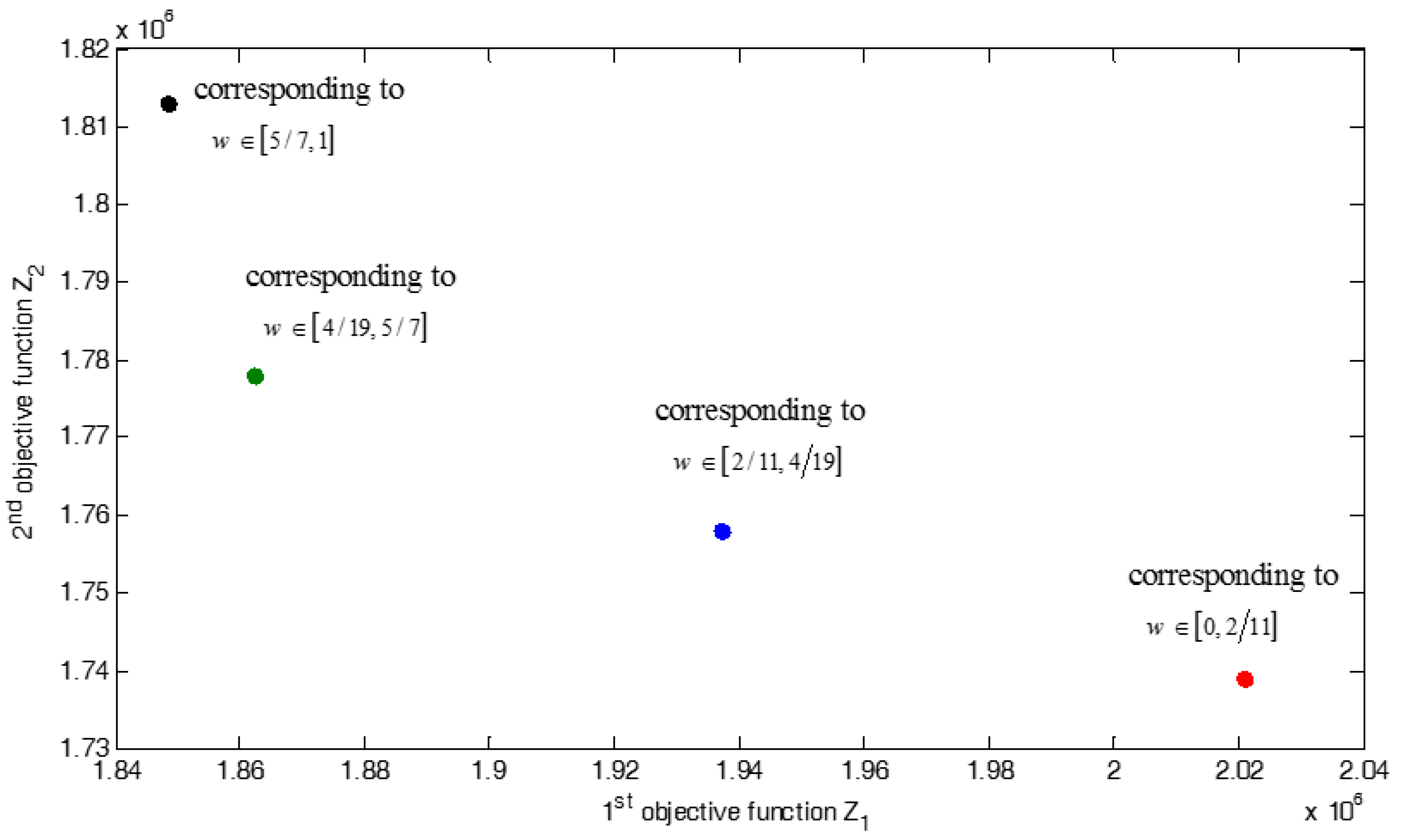
In addition, for the determined efficient solutions, Figure 4 declares the objectives space which represents the complete frontier of the four-index transportation problem.

From Figure 1, the proposed algorithm can locate four alternatives for the original multi-objective four index transportation problem, which constitute the Pareto frontier: $\overline{z}=\left(\mathrm{2,021,100}, \mathrm{1,739,000}\right)$ corresponding the weights range [0,2/11), $\overline{z}=\left(\mathrm{1,937,350},\mathrm{1,758,000}\right)$ corresponding the weights range [2/11,4/19), $\overline{z}=\left(\mathrm{1,862,350},\mathrm{1,778,000}\right)$ corresponding the weights range [4/19,5/7), and $\overline{z}=\left(\mathrm{1,848,350},\mathrm{1,813,000}\right)$ corresponding the weights range [5/7,1), which exhaustively cover all the parameter domain [0, 1]. We also observed that the proposed algorithm locates all the set of nondominated solutions, avoiding solving the large scale problem by transforming it to smaller size subproblems, which can be solved efficiently using any available software package.

6. Analysis of Computational Complexity

In this section we investigate the computational complexity of the proposed algorithm which deals with multi-objective multi-index transportation problem. The algorithm converts the multi-objective formulation to a single objective formulation, and hence decomposes it to a set of two-index transportation problem. In what follows, we assume that the proposed algorithm is to be performed on a set consisting of T sub-problems with n variables. As described in the previous section, the proposed algorithm consists of three main steps. First, transforming multi-objective formulation to single objective formulation. Second, applying decomposition technique to generate T subproblems. Third, solving each sub-problem. As a result, we show that the proposed method becomes strongly polynomial time solvable; the computational complexity in terms of the number of arithmetic operations is O(n3LT), where n is the number of variables, L is the input size of the problem, and T is the number of sub-problems. The suggested approach also has a better computational complexity than the other one dealing with the original four-index problem. This makes the proposed approach computationally cheap due to the decomposition process.

7. Conclusions

In this paper, a mathematical formulation of multi-objective multi-dimensional transportation problem is defined. Moreover, an efficient algorithm is proposed for solving the four-index transportation problem. The proposed algorithm implements the weighting sum method for transforming a multi-objective four-index formulation to a single objective four-index formulation, hence a decomposition approach was applied to decompose the problem to a set of two-index transportation sub-problems, which can be solved efficiently with any suitable software package. On the other hand, the stability set of the first kind is applied in order to determine the weight parameter ranges that keep the optimal solution unchanged. The proposed algorithm can effectively detect all the efficient solutions of the multi-objective four-index transportation problem. Finally, a numerical simulation demonstrates the ability of the proposed algorithm to deal with a multi-objective four-index transportation problem easily. The main features of the proposed algorithm are as follows:

(a)

Capable of decomposing the main problem with four-index into a set of sub-problems with two dimensions, which can be easily solved.

(b)

Capable of detecting all the set of nondominated solutions to the original problem.

(c)

Capable of dealing with low dimensional problem decreasing the time complexity.

(d)

Capable of determining the ranges of the weighted parameters that keep the optimal solution unchanged.

Until now, the multi-index transportation problem is one of the most adaptable transportation problems for engineering and industry applications. Following this direction of research, in the future, we will develop a multi-index formulation for real world application under uncertainty with fuzzy parameters.