Navigation of Autonomous Light Vehicles Using an Optimal Trajectory Planning Algorithm
by
 , ,
, ,
Ángel Valera
1 ,
,
Francisco Valero
2,
Marina Vallés
1,
Antonio Besa
2 ,
,
Vicente Mata
2 and 
Carlos Llopis-Albert
2,* 1
Instituto de Automática e Informática Industrial (ai2), Universitat Politècnica de València, 46022 Valencia, Spain
2
Center of Technological Research in Mechanical Engineering, Universitat Politècnica de València, 46022 Valencia, Spain
*
Author to whom correspondence should be addressed.
Sustainability 2021, 13(3), 1233; https://doi.org/10.3390/su13031233
Submission received: 18 December 2020
/
Revised: 18 January 2021
/
Accepted: 20 January 2021
/
Published: 25 January 2021
(This article belongs to the Section Sustainable Transportation)
Abstract
:Autonomous navigation is a complex problem that involves different tasks, such as location of the mobile robot in the scenario, robotic mapping, generating the trajectory, navigating from the initial point to the target point, detecting objects it may encounter in its path, etc. This paper presents a new optimal trajectory planning algorithm that allows the assessment of the energy efficiency of autonomous light vehicles. To the best of our knowledge, this is the first time in the literature that this is carried out by minimizing the travel time while considering the vehicle’s dynamic behavior, its limitations, and with the capability of avoiding obstacles and constraining energy consumption. This enables the automotive industry to design environmentally sustainable strategies towards compliance with governmental greenhouse gas (GHG) emission regulations and for climate change mitigation and adaptation policies. The reduction in energy consumption also allows companies to stay competitive in the marketplace. The vehicle navigation control is efficiently implemented through a middleware of component-based software development (CBSD) based on a Robot Operating System (ROS) package. It boosts the reuse of software components and the development of systems from other existing systems. Therefore, it allows the avoidance of complex control software architectures to integrate the different hardware and software components. The global maps are created by scanning the environment with FARO 3D and 2D SICK laser sensors. The proposed algorithm presents a low computational cost and has been implemented as a new module of distributed architecture. It has been integrated into the ROS package to achieve real time autonomous navigation of the vehicle. The methodology has been successfully validated in real indoor experiments using a light vehicle under different scenarios entailing several obstacle locations and dynamic parameters.
1. Introduction
In recent years, the fields of application of robotics have grown enormously. Thus, in addition to typical industrial applications (pick and place, arc or spot welding, machine tending, etc.), nowadays robots are being adopted in fields such as medicine [1,2], along with assistance robots [3,4], rescue robots [5], robots that replace human operators in inaccessible or dangerous environments [6], etc. All these tasks have in common uncontrolled and unpredictable environments. Furthermore, cooperation between different robotic systems is usually required for the successful accomplishment of these missions.
In the same way, there has been a very rapid growth in the development of applications based on mobile robots, such as cleaning and inspection robots, robotic transportation systems, precision agriculture, surveillance and military applications, etc. In all of these, one of the most critical problems is autonomous navigation.
The architecture of autonomous navigation in vehicles is based on different complex systems ranging from localization (determining the vehicle position and orientation) [7], perception (acquiring information from its environment and robotic mapping) [8], navigation and planning (guidance of a vehicle from a starting point to a destination through an optimal route while avoiding obstacles) [9], and the control system (managing all devices and systems) [10,11]. The emergence of new technologies such as the Internet of Things (IoT) allows a vehicle to access a great deal of high-quality information [12], which leads to the next generation of intelligent transportation systems with improved accuracy and robustness [13]. This wireless connectivity enables communication with external and internal sources of information, such as sensors, which lead to vehicle-to-vehicle (V2V), vehicle-to-infrastructure (V2I), vehicle-to-sensor, and vehicle-to-internet communications [14].
The communication needed to integrate such information has been tackled in the literature through different procedures, such as middleware or component-based frameworks [15]. A middleware can be defined as “the software layer that lies between the operating system and applications on each side of a distributed computing system in a network” and provides a common programming abstraction through distributed systems [16], improving portability, reliability and reducing the complexity of the systems [17]. In this regard, the use of robot control middleware avoids the problems and limitations of traditional approaches. This is because middleware offers a set of tools and generic libraries, kinematic and dynamic modeling algorithms for robots, control systems, etc. They are systems with increasingly modular structures [18] which allow complex distributed systems that can perform tasks such as hardware and software integration [19]. Moreover, another advantage of some of this middleware is the way the code is developed since the component-based software development (CBSD) approach is used. Therefore, middleware promotes the reuse of software components, thus allowing the implementation of robot systems from other existing ones and minimizing development and maintenance time [20,21].
In the area of robotics there are numerous robot control types of middleware, which include approaches such as Robot Operating System (ROS) [22], Orocos [23], Orca [24] Player [25] or Brics [26]. In this sense, because ROS is component-based free software middleware that has many tools and functionalities useful in the development of robotic applications, ROS outperforms other algorithms when applied to vehicle control, the merging of data from multiple sensors and the timestamping of various devices [27].
Autonomous vehicle localization has usually been addressed by means of the Global Positioning System (GPS) because of its low cost and easy accessibility. However, due to poor reliability, multiple limitations and inadequate accuracy (~10m), in recent years different sensors have been applied for vehicle localization using each standalone sensor, or a combination of sensors. This combination can be performed by means of certain fusion techniques, such as Kalman filter, particle filter, Bayesian network and Dempter-Shafter [7,28,29]. This fusion is translated into a reduction in uncertainty, increase in accuracy and reliability, extended spatial and temporal coverage and improved resolution. The different sensors include vision-based sensors such as cameras, Light Detection and Ranging (LIDAR), Radio Detection and Ranging (RADAR), Infrared (IR), Inertial Motion Units (IMU), wheel encoders, and ultrasonic sensors. An exhaustive summary of the pros and cons of such techniques can be found in [28,29].
Moreover, these sensors combine both on-board and off-board information (such as road marks or real-time traffic data) to avoid harsh environmental situations (e.g., snow, night vision, shadows, illumination variation, etc.), obstacles, pedestrians, other vehicles, etc. [28].
Map matching is the procedure for obtaining the location of the vehicle regarding an underlying map, which encompasses different layers. This covers the static elements of a map (e.g., road network, buildings, etc.); quasi-static features (e.g., road-side infrastructure, etc.); transient dynamic data (e.g., weather and traffic light information, congestion levels, etc.); and highly dynamic data (Vehicle-to-Everything (V2X) communications, Road-side Units (RSU), etc.). Map matching entails a high computational cost and is solved using different techniques such as Markov localization systems and Simultaneous Localization and Mapping (SLAM) systems [30]. There are two main categories of map, i.e., planar maps that are based on layers or planes on a Geographic Information System (GIS); and point-cloud maps which are based on a set of data points in the GIS, which are used in cameras, LIDAR and RADAR sensors. The object recognition and feature matching used to detect, recognize and classify objects is carried out using different methods such as Oriented Fast and Rotated BRIEF (ORB), Binary Robust Invariant Scalable Keypoints (BRISK), Difference of Gaussians (DoG), and Speeded-Up Robust Features (SURF) [31].
The navigation and planning problem can be classified into local and global navigation. The global navigation strategy entails a complete known environment, while the local navigation strategy implies an unknown and partially known environment. There are a wide range of algorithms to address the navigation problem in dynamic environments such as Differential Evolution (DE), Harmony Search (HS), Bat Algorithm (BA), Invasive Weed Optimization (IWO), Ant Colony Optimization (ACO), Bacterial Foraging Optimization (BFO), and Probabilistic Cell Decomposition (PCD) [30]. Furthermore, there are algorithms in the literature for obstacle avoidance, including the Bug algorithm, the Vector Field Histogram (VFH), and the Virtual Force Field (VFF) algorithm [30].
The main and innovative contribution of this manuscript is the development of an optimization procedure for the navigation of mobile autonomous robots while considering energy consumption, the vehicle’s dynamic behavior and avoiding obstacles. The reduction in energy consumption allows companies to fulfill environmental regulations and stay competitive in the marketplace. Furthermore, the disruptive effect of Electric Vehicles (EVs) in the global market could also benefit from energy efficiency. The capabilities of the proposed technology are translated in terms of sustainability covering economic, environmental, and social aspects. In this sense, the methodology is in line with circular economy trends, governmental environmental regulations, and social demands.
In addition, a global trajectory generator algorithm has been implemented and integrated with the ROS packages needed for autonomous navigation. Finally, the parameters of all packages have been tuned. It is a modular solution that provides a distributed architecture for obtaining an efficient and collision-free trajectory. A laser sensor is used not only to generate the environment map, but also to detect and avoid dynamic obstacles.
The paper is organized as follows. The second section presents the car-like vehicle used for the autonomous navigation. The third section describes the procedure developed for the generation of efficient trajectories and carries out a comparison with current state-of-the-art of autonomous vehicle driving. The fourth section presents the software control architecture. It is based on the ROS middleware, and the software integration is presented. The fifth section presents the application developed for the navigation of autonomous light vehicles. The sixth section introduces a discussion of the results. Finally, some conclusions are presented.
2. The Car-Like Light Vehicle RBK
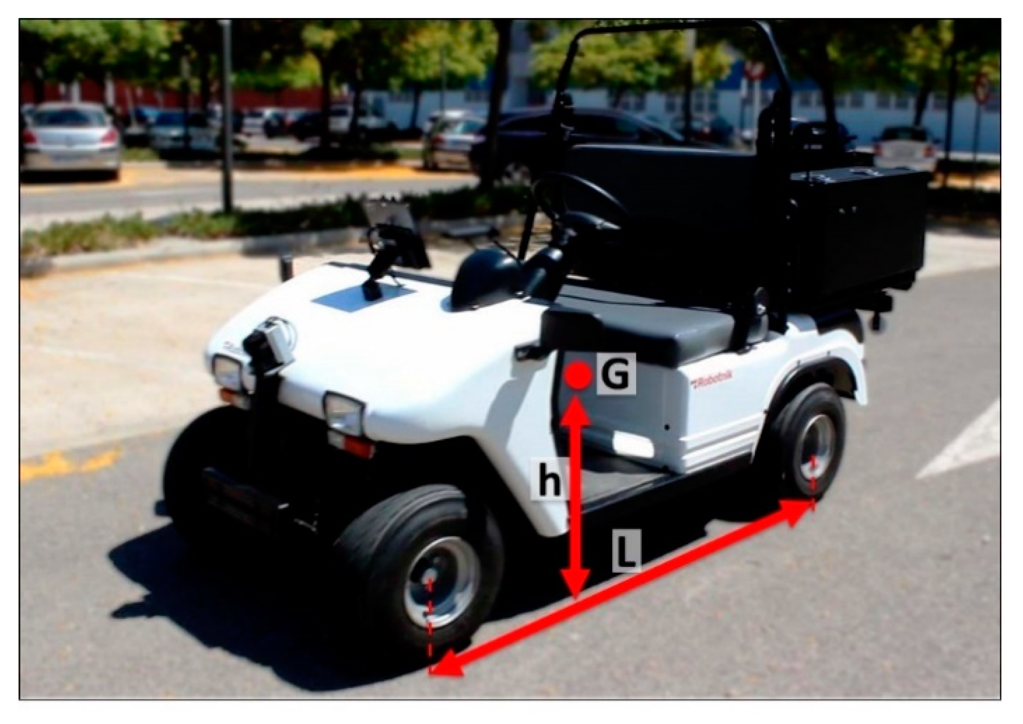
The RBK system is an electric vehicle for people and freight transport. It is powered by a hydrogen fuel cell and batteries with autonomous operation capacity (Figure 1). It has a rear-wheel drive, front-wheel steering Ackerman kinematics, and its main features are power 3.3 kW, mass 690 kg, top speed 32 km/h, length 2.66 m, width 1.23 m, height 1.70 m, wheelbase L = 1.65 m, height of the center of gravity (G) h = 0.50 m, distance from G to the front axle La = 1.10 m, and distance from G to the rear axle Lb = 0.55 m.
Modelling the dynamics of this vehicle has been performed using the bicycle model (see Figure 2). In [32] it is defined in more detail. This paper considers the following simplifications: (a) roll and pitch movements and side-load transfer are not considered, (b) aerodynamic effects are not considered, (c) a plane model of three degrees of freedom has been used, (d) the steering angle has a restriction related to its maximum value, (e) the front wheels are simplified into one that will exert force corresponding to both, (f) the rear wheels have the same simplification, (g) the steering angle corresponds to that of the single front wheel of the model, and (h) the sideslip angles and their gradient are small.
2.1. RBK Actuators and Sensors
To control vehicle movements, it is necessary to control the steering system, brakes, and engine speed. To do this, the RBK mobile robot has a DC motor to change the angle of the vehicle steering wheel in order to change the direction of travel. On the other hand, as mentioned above, the vehicle is propelled by a 3.3 kW AC motor.
The vehicle is equipped with a Curtis AC induction motor controller that provides information such as the controller state, the instant vehicle speed or the steering angle. With this information, the vehicle control algorithm can indicate the desired steering angle, the speed of the steering angle, and the speed and acceleration of the electric car.
The RBK is equipped with two types of sensor, proprioceptive (internal) sensors, which establish its configuration in its own set of coordinate axes, and exteroceptive (external) sensors, which allow the vehicle to position itself relative to its environment.
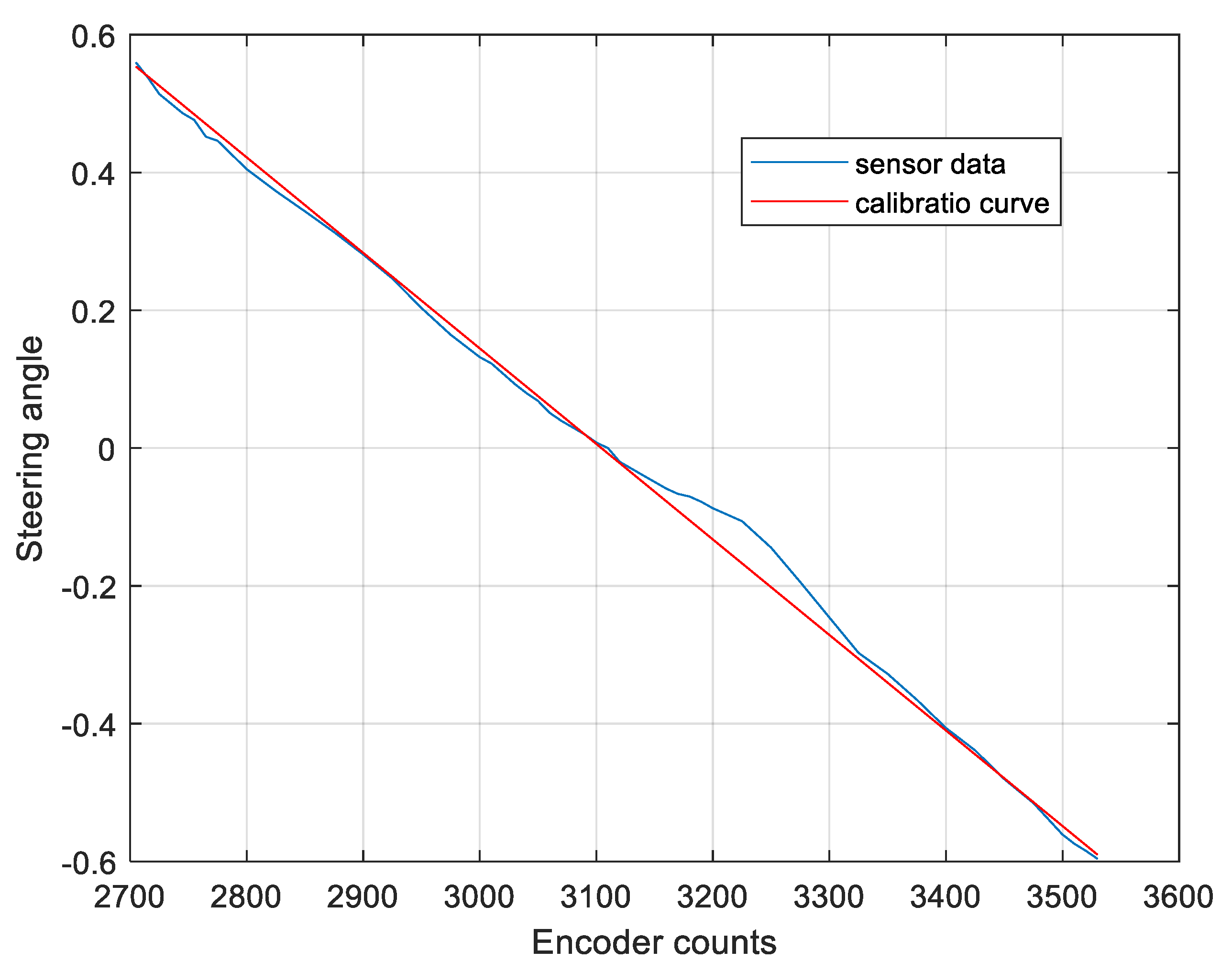
The car-like vehicle has several proprioceptive sensors. The AC motor for vehicle traction has an incremental encoder, and the steering system has an absolute encoder of 12 bits of resolution for measuring the vehicle’s steering angle. In this work, it was necessary to calibrate the steering sensor. Figure 3 shows the encoder and the angle information, and the calibration obtained. The square of the correlation coefficient obtained for the sensor calibration was R2 = 0.9985.
The RBK exteroceptive sensors used for this work are described below.
2.1.1. Racelogic VBOX3i
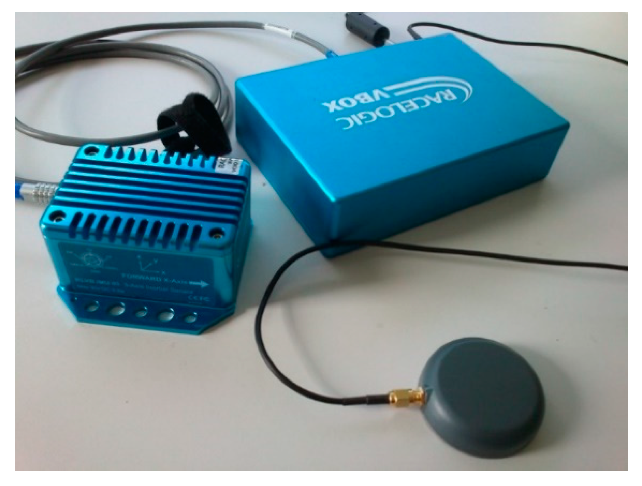
In order to improve the navigation of the vehicle, an inertial measurement unit (IMU) has been used. This is based on VBOX3i from Racelogic [33]. Using a powerful differential GPS engine, the VBOX3i can log GPS and other data (like position, velocity, heading, lateral and longitudinal accelerations, etc.) at 100 Hz. The VBOX3i also includes four high-resolution (24-bits) analogue input channels to record data from external sensors, brake/even trigger input of 10ns resolution, USB interface and 2 CAN bus interfaces to allow connection of Racelogic input modules while simultaneously transmitting GPS data on the second bus. VBOX3i is also compatible with different peripherals, including inertial measurement units, yaw rate sensors, telemetry modules, etc.
VBOX3i incorporates the IMU unit RLVBIMU04-V2 (see Figure 4). This provides highly accurate measurements of the accelerations and angular velocities using three accelerometers and three rate gyros. The acceleration range is ±5 G with a resolution of 0.04mg. The angular velocity range of this IMU unit is ±450°/s, with a resolution of 0.00085°/s. The Controller Area Network (CAN) based unit is temperature compensated and has improved calibration and stability. This IMU is designed for use either as a standalone sensor with simple connection and configuration via the CAN bus interface, or for use with VBOX GPS data loggers.
In this work, a software package had to be programmed in order to supply the information from this sensor to the vehicle control software. Using a serial communication port, the VBOX3i sends to the vehicle control PC the X, Y and Z axes’ accelerations and the pitch, roll, and yaw rate at a frequency of 20Hz.
2.1.2. SICK LMS291 Laser Sensor
The LMS291 Laser Measurement Systems is a non-contact measurement system (NCSDs) in stand-alone operation for industrial applications [34]. The system scans its surroundings two-dimensionally with a radial field of vision using infra-red laser beams. The measured data can be individually processed in real-time with external evaluation software for determining positions and other measurement tasks.
The laser measurement system can be used for determining the volumes or contours of bulk materials, determining the volume and the position of objects, collision prevention for vehicles or cranes, controlling docking processes, classification of objects, process automation, monitoring open spaces, etc.
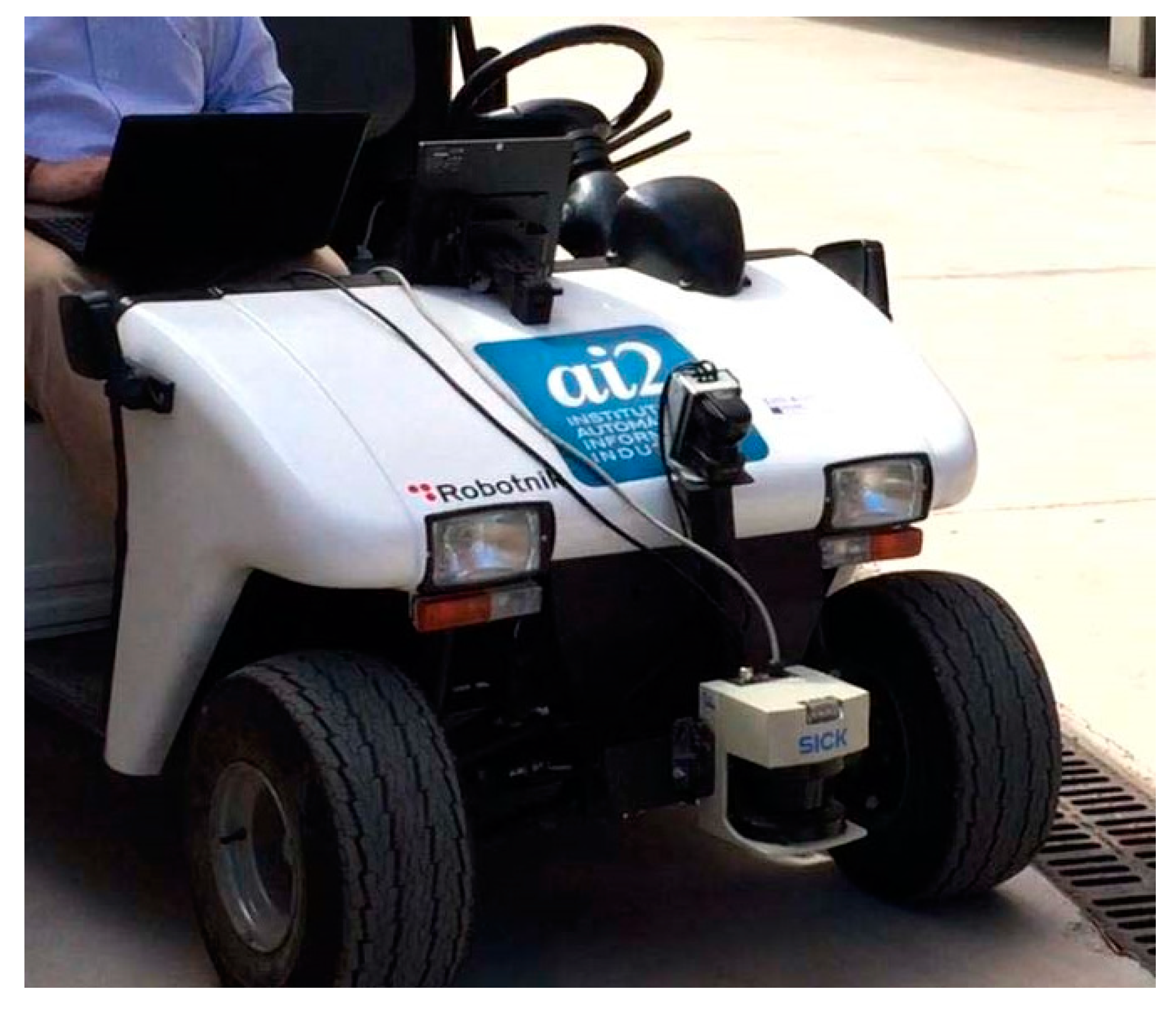
In this work, the laser sensor has been located in the front of the vehicle (see Figure 5). The sick_scan package [35] was used to install and program the LMS291 laser sensor. This driver provides the measurement data as a point cloud. These data are the distances between the laser sensor and the objects, calculated by measuring the time of flight of laser light pulses.
3. Trajectory Generation
This section shows how the trajectory modeling and a collision-free minimum-time trajectory is obtained.
3.1. Global Trajectory Modeling
The objective of the global trajectory planning problem is to obtain, with the constraints associated with the technical characteristics of a given vehicle, a trajectory that connects the starting and ending positions through a series of waypoints in minimum time.
From this series of points, a trajectory will be adjusted by means of the interpolation functions (1), so that it is carried out in minimum time, complying with pre-established restrictions. To accomplish this, a non-linear optimization problem is established. Considering the objective function and non-linear constraints, the problem is then defined.
For modeling the trajectory, the center of gravity of the mobile robot must pass through a sequence of m, via points (initial and final more waypoints) joined by m − 1 polynomial sections:
∀t ∈ [0, tj], where j = 1 …m − 1, t being the time variable associated with the robot’s motion in the polynomial section.
The (m − 1) polynomial functions that make up the path should be set up according to the (8 (m − 1)) continuity conditions shown below:
- C0 continuity: the initial position of each section must be equal to the final position of the previous one. Hence, the final position of each section must coincide with the initial position of the following section. With this condition, (4 (m − 1)) equations are set.
- C1 continuity: the initial velocity of each section must be equal to the final velocity of the previous one. With this condition, (2 (m − 2)) equations are set.
- C2 continuity: the initial acceleration of each section must be equal to the end of the previous one. With this condition, (2 (m − 2)) equations are set.
- The initial and final velocities of the trajectory must be zero. Four equations are set with this condition.
With these conditions and the times associated with the different segments, the coefficients of the polynomials can be obtained by solving a linear system of 8 (m − 1) equations. This process will be repeated every time the optimization algorithm adjusts the time for a given section.
To obtain the global trajectory of minimum time per m via points, an optimization problem with non-linear constraints has been proposed. For this optimization problem, the following constraints have been considered:
- The initial orientation of the robot θi, corresponding to the initial position.
- The steering wheel angle does not exceed the specified value δmax.
- The maximum velocity of the vehicle cannot exceed Vmax.
- The driving force is limited by the torque curve of the engine.
- The adhesion of the tires to the terrain is limited.
- The energy consumed by the vehicle is limited.
In this work, the solution is obtained by the NLPQLP Quadratic Programming Algorithm with Distributed and Non-Monotone Line Search (see [36]) considering the objective function:
It should be noted that, in order not to penalize the computation time, in each iteration the linear system will be solved using the normalized time method. In addition, finite differences are used for the calculation of the derivatives of the constraints.
In [37,38], the mathematical approach to the path generator used in this work is shown in greater detail. It shows the kinematic and dynamic modeling of a “bicycle model”, the formulation of the constraints, and the procedure for obtaining the global trajectory. It also shows how to obtain a path free of collisions with static obstacles, showing the simulation of various trajectories. It should be noted that these benefits are improved in this paper, since it will be possible to modify this efficient trajectory with restricted energy consumption, to avoid collisions with mobile obstacles [39].
3.2. Collision-Free Global Trajectory Generation
This Section presents the generation of an efficient and collision-free trajectory for a mobile robot in an environment with static obstacles. A trajectory is efficient when it is near the minimum time with a low computational cost and it matches the constraints imposed on the robot, as defined in Section 3.1. For collision detection (see [22]), the robot is modeled as a rectangular parallelogram and the environment is discretized by means of pattern obstacles, resulting in a very efficient procedure.
The trajectory generation algorithm needs the following initial information:
- The vehicle’s parameters.
- Locations of obstacles.
- Initial position (xGi, yGi) and orientation θGi of the vehicle.
- Final vehicle’s position (xGf, yGf).
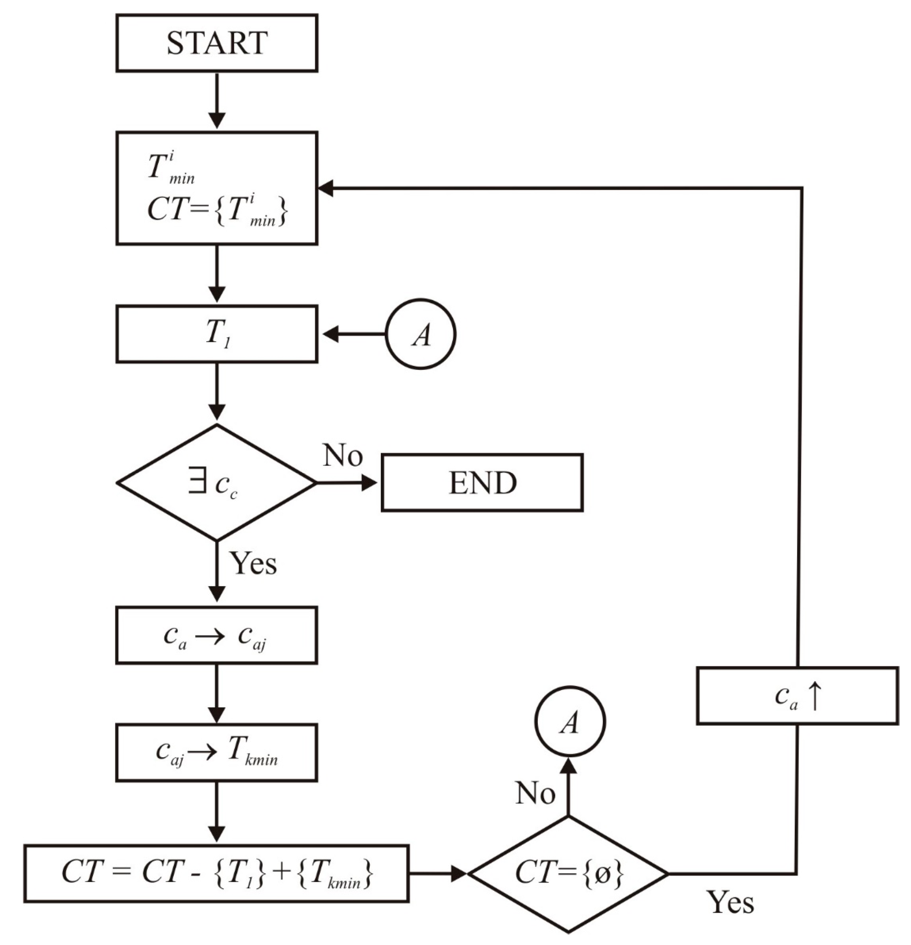
The algorithm for collision-free path generation is an iterative procedure with the following steps:
- Calculation of the minimum-time trajectory in a single section that passes through the initial (xGi, yGi) and final (xGf, yGf) points. is added to the set of trajectories pending verification and ordered from smallest to longest time, CT.
- Search for collisions in the minimum time trajectory . If there is a collision cc, a previous point ca in is determined, otherwise is the solution.
- If cc belongs to section m of T1 and ca to m − 1, T1 is extracted from CT and goes to point 7.
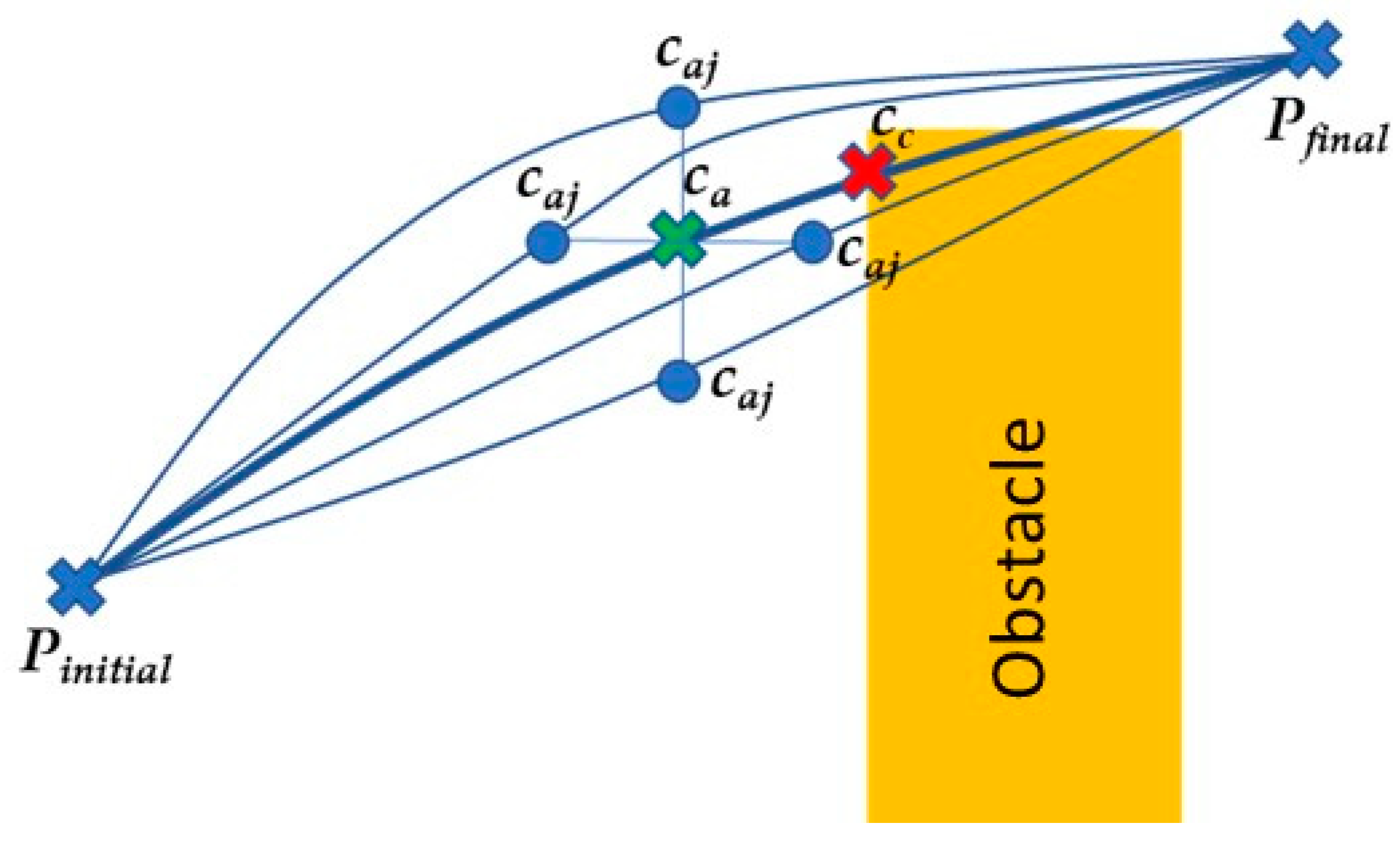
- Generation of adjacent positions from ca: four locations around ca are generated (caj, j = 1 … 4). (see Figure 6).
- Generation of offspring trajectories: for each of the adjacent positions obtained at previous point, caj, an offspring trajectory Tkmin (0 < k ≤ 4) is calculated, which contains all the passing points of previous to ca, point caj and the end point of the generating trajectory (xGf, yGf).
- CT update: the trajectory is extracted and the Tkmin generated in the previous section are added, reordering its elements from smallest to longest time.
- Blocking check: if CT is an empty set, return to step 2 by performing and increasing the step to obtain . Otherwise, return to step 2 without modifying CT.
The collision-free path generation algorithm proposed is highlighted in Figure 7.
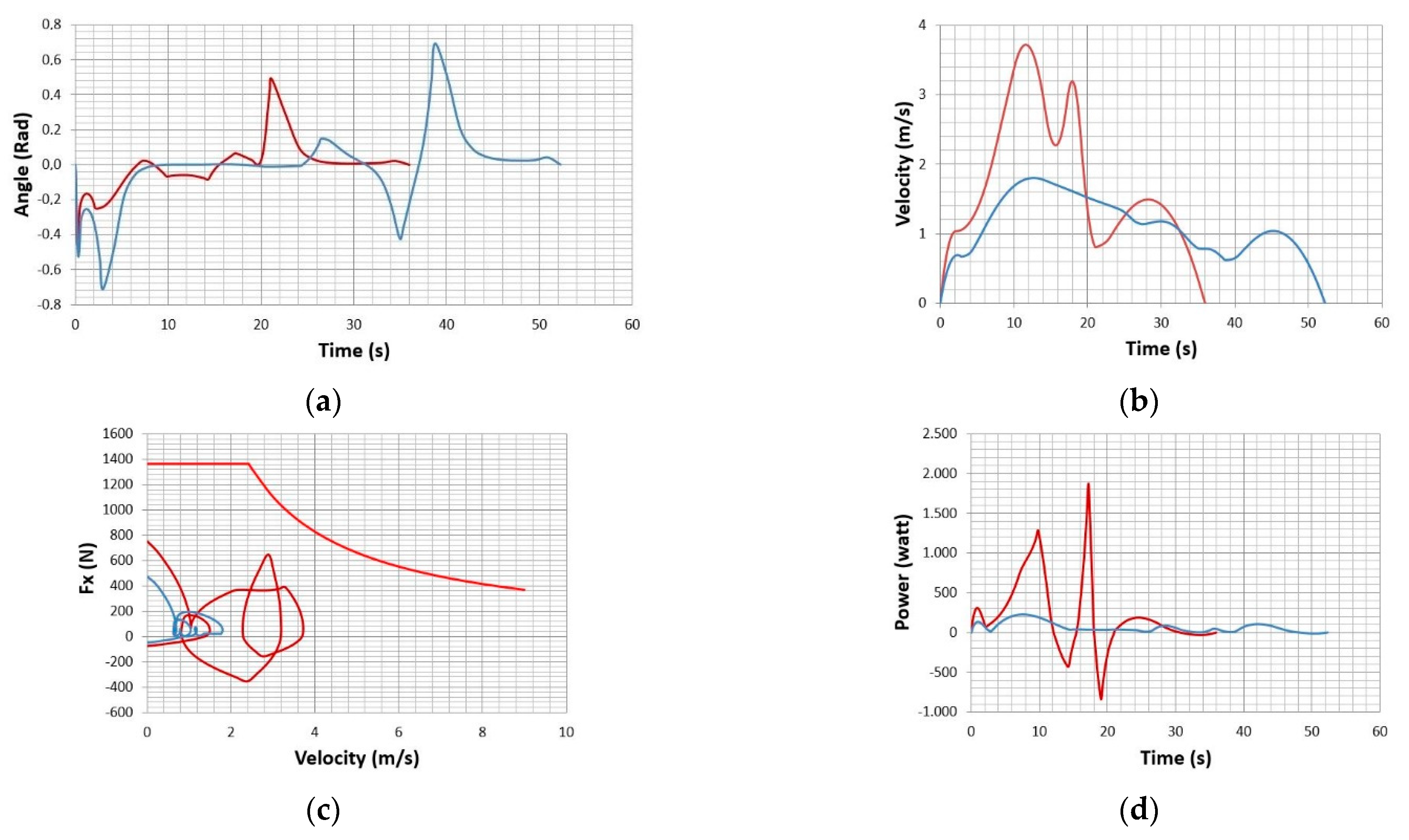
To illustrate this procedure, an example is shown in which, for the same workspace and with the same start and end positions, different limits are set for the energy consumed in the trajectory. Case 1 considers a consumption limitation of 10,000 Joules. In Case 2, the consumption was limited to 3500 Joules. Table 1 provides the most significant results and Figure 8 shows the paths for both cases.
Figure 9a shows how the constraint acts on the steering in the low-velocity trajectory that makes tighter turns. Figure 9b shows the evolution of the velocity in each trajectory, which is higher for the trajectory with higher energy consumption. The evolution of the driving force with the velocity of the robot is shown in Figure 9c, where the limit imposed by the motor has been indicated in red, and it can be seen how the constraint works for Case 1. Figure 9d shows the power applied to the rear wheels along the trajectory, which will be positive when supplied by the engine and negative when braking. The integration of the positive part allows us to obtain the energy consumed. Again, it is worthwhile mentioning that, although there are other approaches for autonomous vehicle path planning [40], the main difference of the present work regarding these algorithms is its capability to optimize vehicle navigation while considering energy consumption, together with typical vehicle dynamic behavior and obstacle avoidance.
3.3. Comparison with the Current State-of-the-Art of Autonomous Vehicle Driving
A comparison with the current state-of-the-art of autonomous vehicle driving is presented in Table 2. An exhaustive literature review can be found in [41,42,43]. This shows a wide range of techniques for global and local planning, and for modelling the dynamic behavior of the vehicle, each one with its pros and cons. There is also a broad variety of methods for location and mapping, control systems and perception sensors. As a result, the approaches presented by different authors for autonomous vehicle navigation entail a combination of such techniques, each one with its own advantages, disadvantages, and limitations. For instance, some approaches only consider static obstacles or are limited to static environments; present a high computational cost; assume low or constant speed; the tests are carried out with a miniature-sized vehicle; no collision checking is performed; obstacles are treated as simple geometries; lateral accelerations and curvature constraints are omitted; only lane-change maneuvers are considered; a large amount of data are needed; a traffic-free environment without regulations is assumed; optimization sensitivity to a number of variables and constraints, presenting problems with vehicle dynamics or in the curvature, lead to errors in the presence of obstacles; motion is restricted; there are difficulties in dealing with evasive maneuvers, etc. As aforementioned, the main difference of the present work regarding the current literature is its capability to optimize vehicle navigation while considering energy consumption, together with the typical vehicle dynamic behavior and obstacle avoidance.
4. Software Control Architecture
As seen above in the introductory section, autonomous navigation must solve different complex problems related to the location estimation, mapping, trajectory generation, etc. Using a robot middleware based on CBSD allows the saving of development time in the initial start-up part of the experimental platform and focus on the part of the autonomous navigation application under study or development. This is so since it allows the reusing of code already developed and previously validated for handling sensors and actuators, as well as other tasks necessary for autonomous navigation, but different from those under evaluation.
In this sense, the chosen software architecture for this work is based on the Robot Operating System (ROS) [47]. ROS is robot control middleware that has a fully distributed and modular component-based architecture. It is the most widely used middleware today and has a very large and active developer community. ROS has common features with other robot control middleware like Orocos, Orca, Microsoft Robotics Studio or Player, but, being open-source software (under the Creative Commons Attribution 3.0 license), programmers can freely share, use, and distribute the applications and developments made. In this way programmers can make new applications without having to start from scratch but based on previously tested and validated algorithms and programs.
Although ROS is not an operating system (it was defined as an open-source meta-operational system), it provides the standard services of one, such as hardware abstraction, low-level device control, implementation of commonly used functionality, message passing between processes, package maintenance, etc.
It is based on a network architecture where the processing takes place in the nodes that can receive, send and multiplex messages. The library is oriented for a UNIX system (Ubuntu-Linux) although it is also being adapted to other operating systems such as Fedora, Mac OS X, Arch, Gentoo, OpenSUSE, Slackware, Debian or Microsoft Windows. ROS programming can be done in different languages, such as C++, Python, Octave, JAVA, etc.
ROS has two basic parts: the operating system and a set of tools that are organized into packages that implement different functionalities. A package might contain ROS nodes, a ROS-independent library, a dataset, configuration files, a third-party piece of software, or anything else that logically constitutes a useful module. These packages are contributed by users and aim to provide useful and user-friendly functionalities so that the software can be easily reused.
The communication between the different nodes is governed by the master (ROS MASTER). This communication can be done by message passage (via ROS topics) or by service request.
The messages and service calls do not pass through the MASTER. It first registers all the nodes, and then establishes communication between peers and between all the processes of the system, thus establishing a decentralized architecture.
So, in this work, the robot control middleware ROS has been used to develop an autonomous vehicle navigation based on the trajectory generation described in Section 3. The way the trajectory generation algorithm has been integrated in the navigation application is described in the next section.
5. Development of Autonomous Light Vehicle Navigation
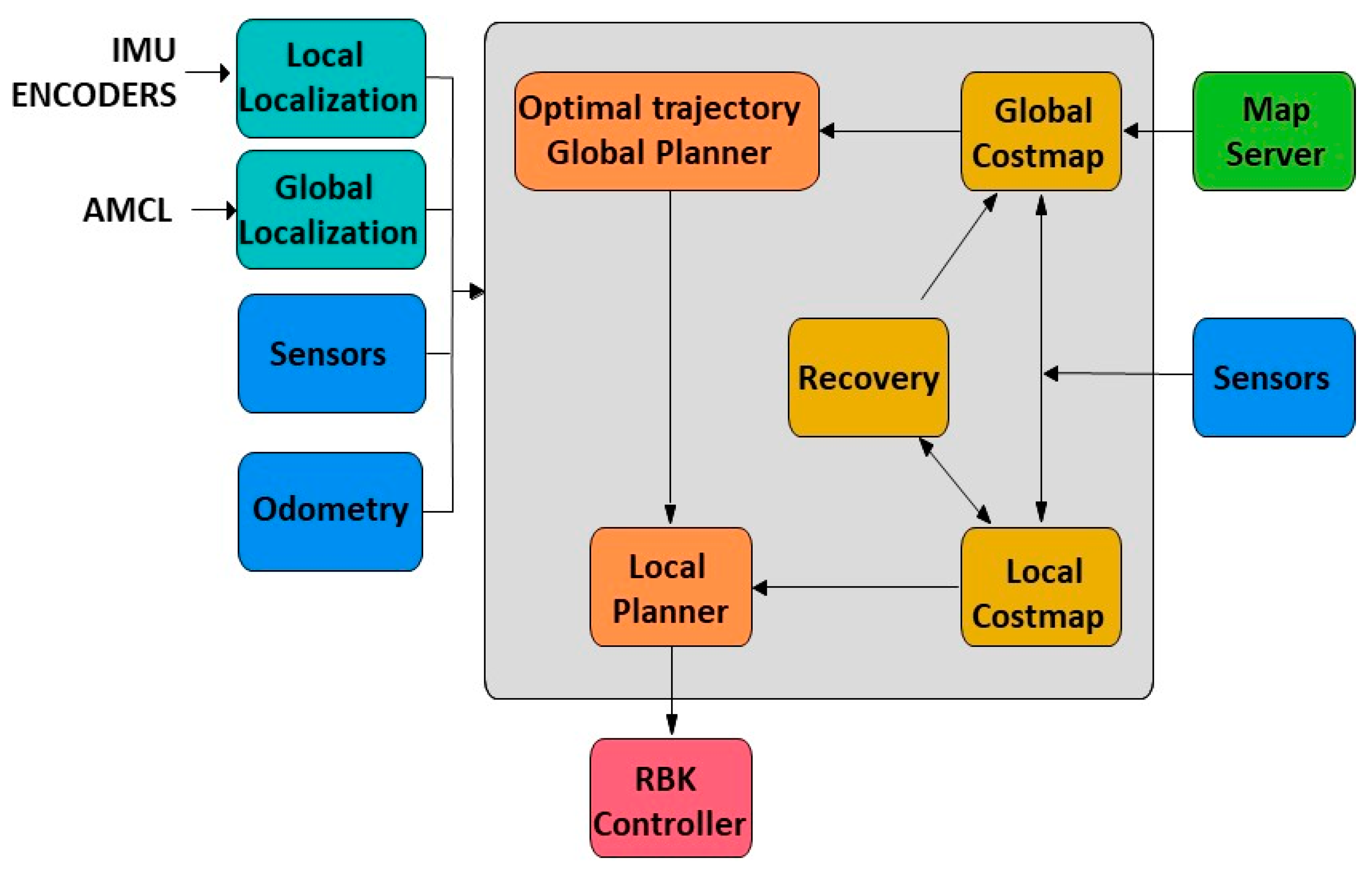
The trajectory generator presented in Section 3 has been integrated in the ROS navigation package move_base [48], which is shaded in gray in Figure 10 where all the modules and relationships needed for autonomous navigation are represented.
The Global Planner module computes the path to be followed by the vehicle to achieve the target position and substitutes for the original Global Planner module that comes with the move_base package provided by ROS. This new module implements the optimization algorithm for modeling the efficient trajectory with constrained energy consumption, proposed in Section 3. This module depends on a global map in which are shown possible obstacles that must be considered by the algorithm to calculate the global path free of obstacles and that is modified dynamically as the vehicle is moving by another application described later. Finally, the module provides (publishes) the trajectory calculated to the Local Planner module. The planner used in this work is The Elastic Band (TEB) developed by the Dortmunt University and provided by the teb_local_planner ROS package. This package receives a list of positions with their orientation and generates a trajectory that the vehicle can follow without problems, based on elastic band behavior.
Using laser measurements and vehicle odometry, the Local Planner can modify the trajectory locally to avoid collisions with dynamic obstacles. This local scheduler sends the necessary control actions to the RBK_controller node to regulate the vehicle’s steering and speed systems.
In addition to the Global Planner and Local Planner modules, a localization system is used that allows the ensuring of where the robot is at all times. The localization system is not included with the original navigation package, so it must be integrated into it.
This localization system will compare the map on which the vehicle will circulate with the data obtained from the laser device. For indoor navigation, it will be made up of two localization systems, the global and the local.
The local localization system works in continuous mode with a higher frequency than the global localization system. It uses the IMU and odometry measures with an Extended Kalman Filter (EKM) to fuse the different sensors’ data. This EKF is implemented by the robot localization package provided by ROS. For use in the autonomous navigation application being developed, such parameters as frequency, sensor timeout and two_d_mode have also been tuned.
For the global localization system, the AMCL algorithm has been used which will return a cloud of points with possible vehicle positions, and each of these points will have a covariance. This one works in discrete mode in such a way that it publishes, from time to time, a position that is used to correct the one given in a continuous way by the local localization system. In order to use this localization method, a map of the area which the robot is navigating and a laser sensor for detecting the environment are needed. To use this algorithm, some parameters (such as Min_particles, Max_particles, Use_map_topic, Odom_model_type, Update_min_d) have been fixed.
In addition to the application that allows navigation, it is necessary to have another application to generate maps. In this work, the slam_mapping package from ROS has been used, and more exactly the gmapping node. As the vehicle starts to move the map begins to be autocompleted.
Taking advantage of the ROS modular architecture, it was only necessary to implement and compile the newly developed module, reusing the modules already developed for the rest of the necessary navigation tasks.
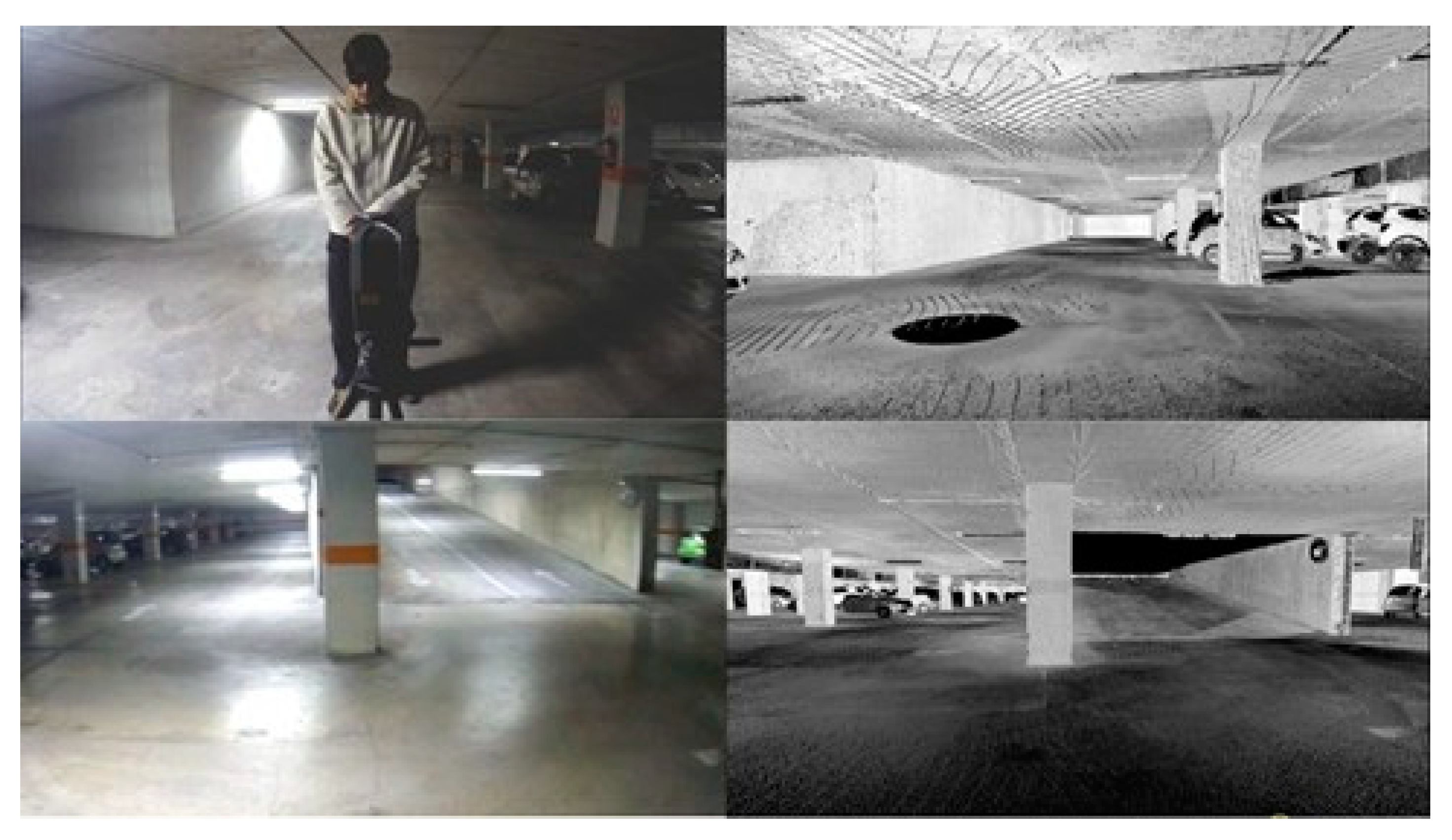
After tests in the laboratory, several experiments were conducted in the indoor and outdoor car garages at Ciudad Politécnica de la Innovación, Universitat Politècnica de València (CPI-UPV) in Spain with satisfactory results. For some of these tests, the indoor garage was scanned with a 3D FARO Focus 3D laser sensor. In the following link a video can be seen showing the process of capturing and finally obtaining mesh points: https://idecona.ai2.upv.es/nuevo_video/mapa-3d-garaje-cpi-u-politecnica-valencia. Figure 11 shows some pictures of the indoor garage and its 3D map.
Because the laser scanner incorporated into the RBK only provides measures in 2D, the 3D point clouds obtained from the garage with the FARO sensor were reduced to a 2D map. In these maps only the walls and the pillars are reflected. The parked cars were removed from the maps as they are considered dynamic obstacles and they should not be considered as part of the static global maps.
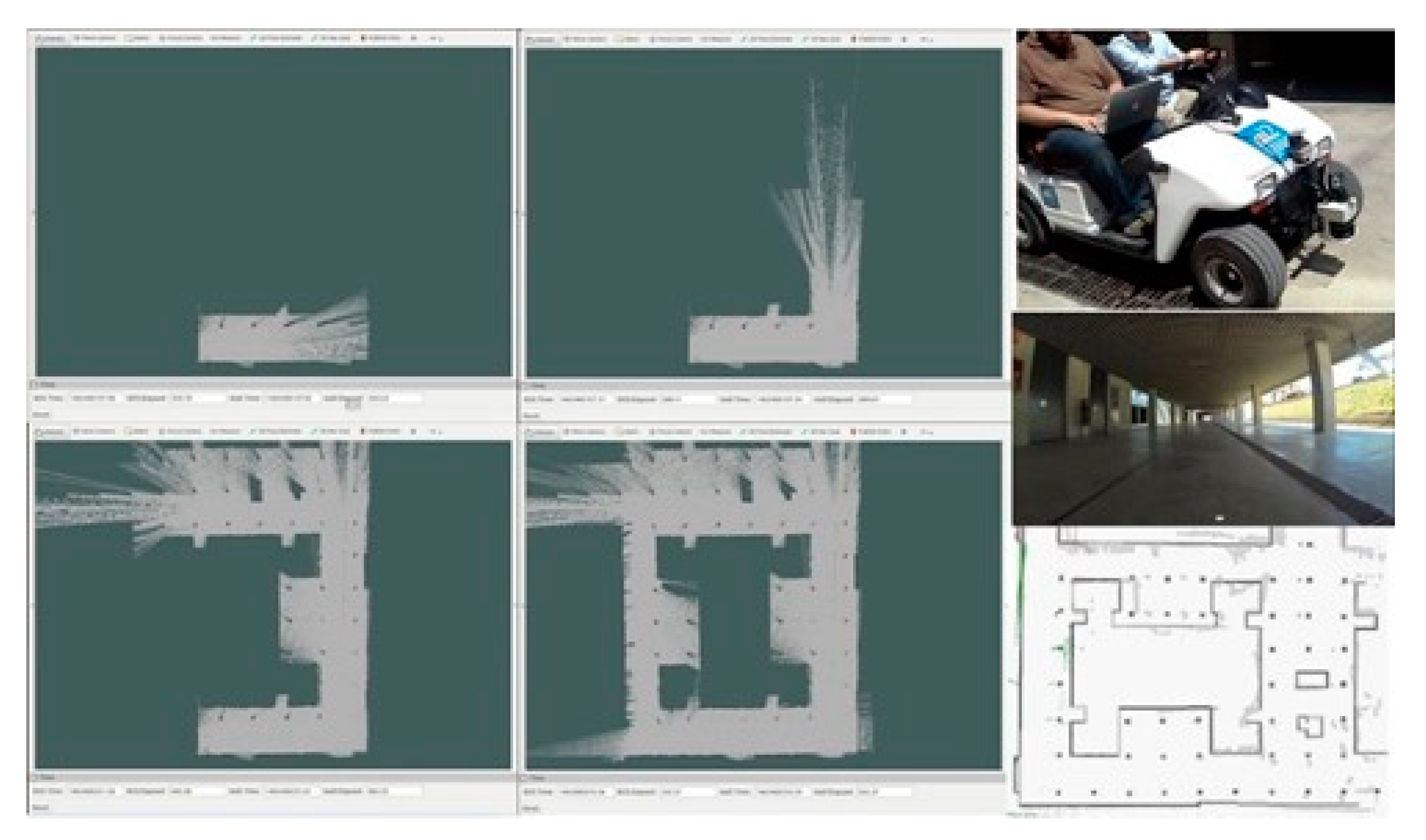
The outdoor garage was scanned in 2D with the SICK sensor laser shipped onto the RBK vehicle. Figure 12 shows the creation of this map. A video with the map generation using this sensor can be obtained at: https://idecona.ai2.upv.es/nuevo_video/maps-generation-autonomous-navigation-vehicles.
6. Results and Discussion
This research goes one step further than the current literature by considering the vehicle’s energy consumption among the constraints of the optimization problem, while minimizing the time required to perform the trajectory and taking into account the typical dynamic behavior of the vehicle and of obstacle avoidance. Furthermore, this is carried out using an efficient and robust algorithm with low computational cost. Another advantage of the proposed system is that it works in two stages, the first with global planning and fixed obstacles, and the second with local planning with mobile obstacle avoidance. In addition, a software control architecture based on ROS middleware is used, which leads to obtaining efficient and safe trajectories as shown in all the tests carried out.
In this sense, in Section 3.2 several cases were successfully conducted to validate the collision-free global trajectory algorithm, which share the same workspace and start and end positions but differ in limits of energy consumed during the execution of the trajectory. These tests show the capability of the algorithm to optimize vehicle navigation while considering energy consumption. This enables the automotive industry to design environmentally sustainable strategies towards compliance with governmental greenhouse gas (GHG) emission regulations and for climate change mitigation and adaptation policies. The reduction in energy consumption also allows companies to stay competitive in the marketplace.
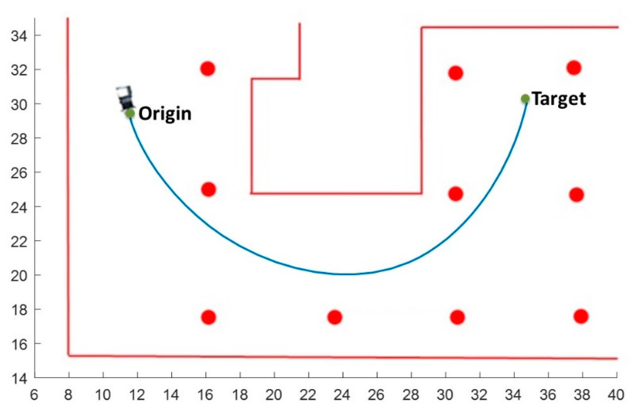
In addition, to validate the navigation system numerous tests were carried out as explained in Section 5 by considering both numerical simulations and an actual electric vehicle. They entail different scenarios in which the position of fixed obstacles, the consideration of several dynamic obstacles and the limitations of the maximum energy consumed were varied, and were performed at the CPI-UPV outdoor garage. Figure 13 shows the first test. This was a simple trajectory from the origin point (11.5, 29.5) to the target point (35, 30). In red the walls and the columns of the garage are represented. The blue line shows the original trajectory generated by the algorithm proposed in this work.
Figure 14 shows the trajectory reference and the path executed by the vehicle. As can be seen, the vehicle follows the reference with a very small error.
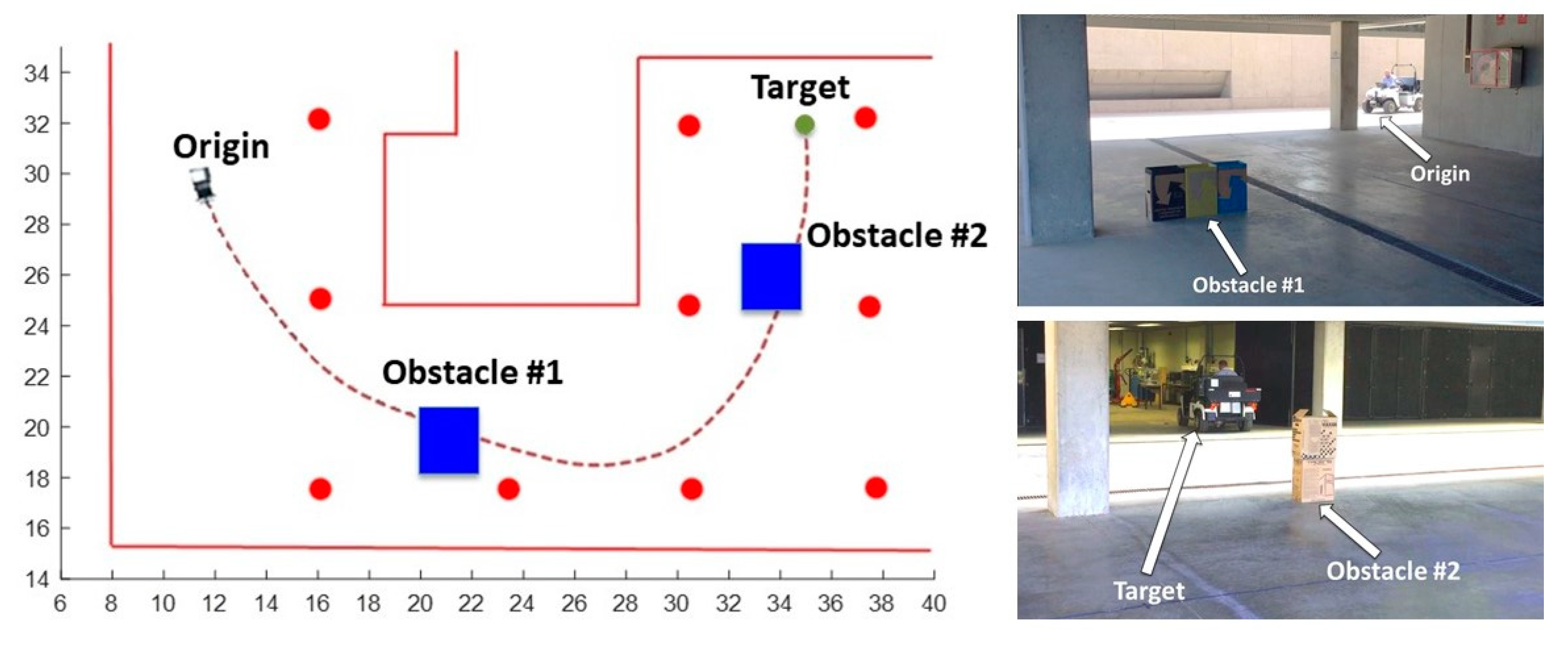
Figure 15 shows the second scenario presented in this work. The original trajectory generated (dashed line) was similar to the path of the first test, but in order to validate the proposed solution two dynamic obstacles have been placed at the navigation trajectory: Obstacle #1 and Obstacle #2.
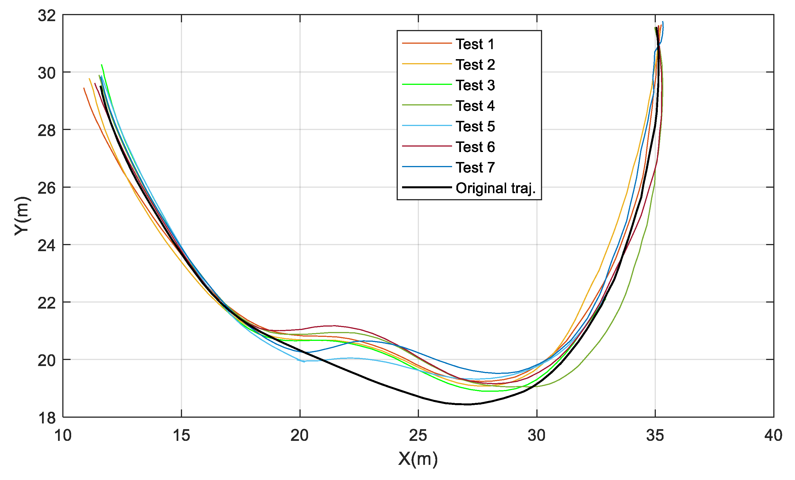
Figure 16 shows the response of the vehicle when only Obstacle #1 was placed. The original trajectory (without obstacle) is represented in black and with double thickness. Hundreds of simulations have been carried out with different scenarios in which the position of fixed obstacles and the limitations of maximum energy consumption were varied. The remaining curves in Figure 16 show seven of these tests performed on the vehicle. The starting position of the tests differs slightly, because it is complicated to place the vehicle in exactly the same original position.
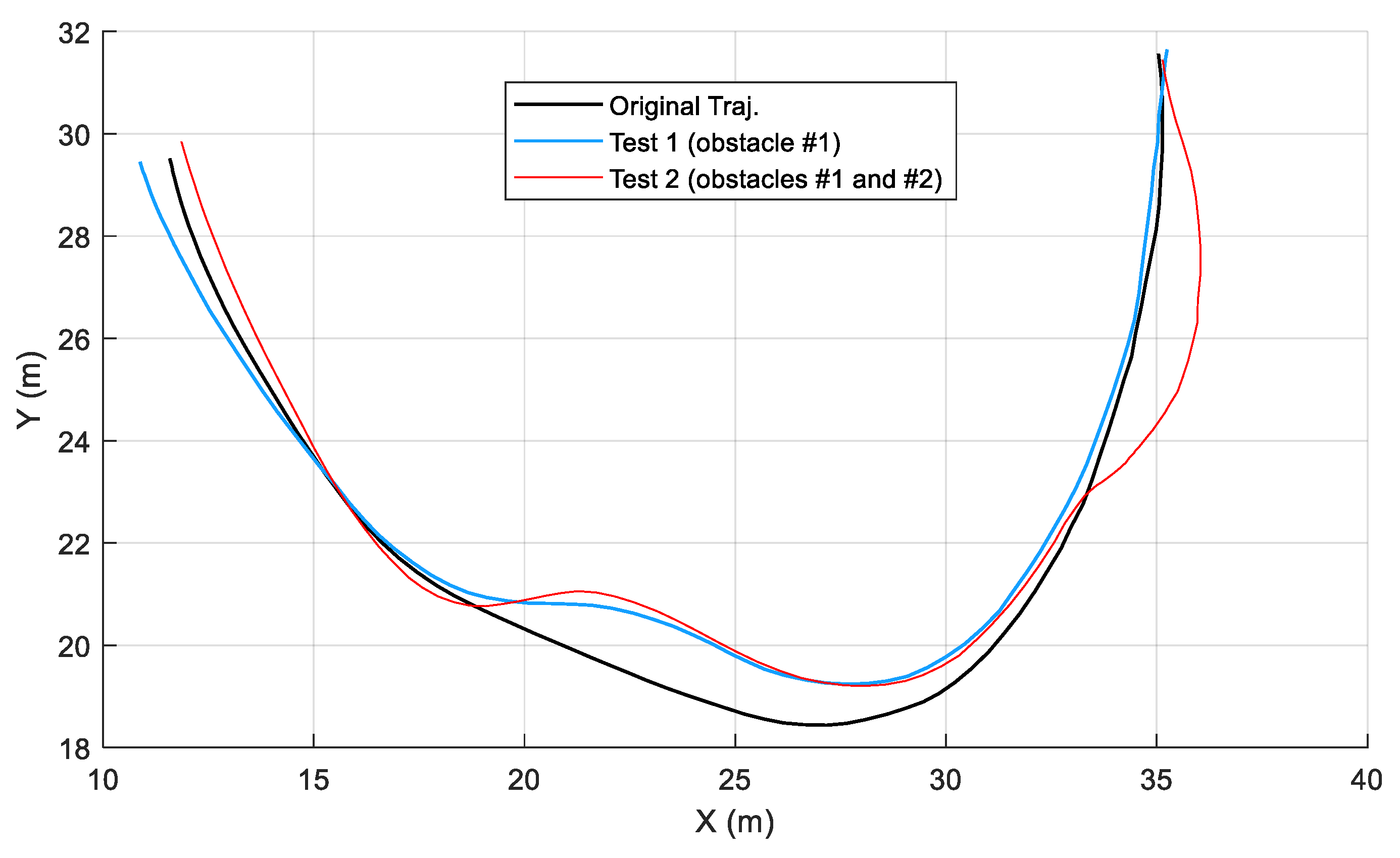
Figure 17 shows the response of the vehicle in a more complex scenario. The original trajectory without obstacles is shown in black, in blue when obstacle #1 was located, and in red when obstacles #1 and #2 were placed.
The complete demonstration of this experiment is available at the following link: https://idecona.ai2.upv.es/nuevo_video/electric-vehicle-automatic-natigation-obstacles-avoidance.
As a result, all these tests have proved the worth of the proposed navigation system. However, the system developed presents several weaknesses and limitations. In this sense, in a few rare cases, the ramification process to avoid obstacles can considerably increase the computational cost of the global algorithm in order to obtain the optimal trajectory, because of falling trapped to a local minimum. The dynamic behavior of the autonomous vehicle does not consider the roll and pitch movements, side-load transfers, and aerodynamics effects. In addition, a more realistic modelling of the steering and sideslip angles could be implemented. Therefore, further research should focus on the one hand on the trajectory generation, and on the other hand the development and implementation of navigation packages. The algorithm should be implemented with some improvements in both the behavior of the tires and in the modelling of losses. Nevertheless, a balance should be sought between the complexity of the models, which affects the computation time, and the accuracy of the results. For dissemination purposes, future work will be to publish a new ROS navigation package in a public directory to allow the scientific community to download and use it. Eventually, this package will be translated into the new version of the Robotic Operating System, ROS2.
Finally, as a conclusion of the comparison with the current state-of-the-art of autonomous vehicle driving as presented in Section 3, the main difference of the present work is its capability of optimizing vehicle navigation while considering energy consumption, together with typical vehicle dynamic behavior and obstacle avoidance.
7. Conclusions
This paper has presented the development and its implementation of an autonomous navigation system for mobile robots. It has shown the hardware/software platform used. The hardware is based on the RBK car-like vehicle equipped with advanced sensors such as a laser rangefinder and an IMU unit. The software platform is based on a distributed CBSD architecture. The software control architecture developed is based on the robot programming framework of the Robot Operating System (ROS).
The main contribution of this paper is the development of an autonomous navigation system for mobile robots while considering energy consumption. This enables the automotive industry to design environmentally sustainable strategies towards compliance with governmental greenhouse gas (GHG) emission regulations and for climate change mitigation and adaptation.
This navigation system consists of two planners. The first (global planner) generates the global path free of collisions which considers the static obstacles (walls, pillars, etc.) that are specified by the global map. The calculated trajectory is provided to the second planner: the local planner. Based on the vehicle’s laser and odometry sensors, this local planner is able to modify the trajectory locally to avoid dynamic obstacles.
The global planner developed in this work has several advantages. It is a collision-free efficient trajectory planner that implements, with a low computer cost, an optimization algorithm capable of modeling the trajectory by specifying the proposed restricted energy consumption.
Several tests have been carried out to validate the proposed planner. These tests took place in the same workspace and with the same initial and final positions, but different limits were set for the energy consumed in the trajectory. The paper has shown how these energy limitations impact on the vehicle’s response, both in steering and velocity.
The new global planner has been integrated and validated in the ROS middleware. In this way, different tasks that make up the navigation algorithm have been programmed as ROS modules. These modules have the ability to communicate between themselves, giving the system great flexibility, scalability and reusability.
This work has also presented some tasks related to the calibration and adjustment of the sensors and actuators of the vehicle, the parameter setting of packages and modules of the ROS, the generation of the environment maps for the navigation, etc.
Finally, several experimental tests of indoor navigation have been carried out. These tests validate the proposed solution, providing very satisfactory results.
Author Contributions
Conceptualization, Á.V., F.V. and V.M.; Data curation, M.V., A.B. and C.L.-A.; Formal analysis, M.V., A.B. and C.L.-A.; Funding acquisition, Á.V. and V.M.; Investigation, F.V. and C.L.-A.; Methodology, F.V., M.V. and C.L.-A.; Project administration, Á.V. and V.M.; Resources, M.V.and A.B.; Software, F.V. and A.B.; Supervision, Á.V. and V.M. All authors have read and agreed to the published version of the manuscript.
Funding
This work has been partially funded by FEDER-CICYT project with reference DPI2017-84201-R financed by Ministerio de Economía, Industria e Innovación (Spain).
Informed Consent Statement
Informed consent was obtained from all subjects involved in the study.
Data Availability Statement
Data is not publicly available, though the data may be made available on request from the corresponding author.
Acknowledgments
The authors sincerely acknowledge Borja Ponz for his help on several technical questions in this work.
Conflicts of Interest
The authors declare no conflict of interest.
References
- Shibata, T. Therapeutic seal robot as biofeedback medical device: Qualitative and quantitative evaluations of robot therapy in dementia care. Proc. IEEE 2012, 100, 2527–2538. [Google Scholar] [CrossRef]
- Lo, A.C.; Guarino, P.; Richards, L.G.; Haselkorn, J.K.; Wittenberg, G.F.; Federman, D.G.; Ringer, R.J.; Wagner, T.H.; Peduzzi, P. Robot-assisted therapy for long-term upper-limb impairment after stroke. N. Engl. J. Med. 2010, 362, 1772–1783. [Google Scholar] [CrossRef] [PubMed] [Green Version]
- Körtner, T.; Schmid, A.; Batko-Klein, D. How Social Robots Make Older Users Really Feel Well—A Method to Assess Users’ Concepts of a Social Robotic Assistant; Springer: Berlin/Heidelberg, Germany, 2012. [Google Scholar]
- Mukai, T.; Hirano, S.; Nakashima, H.; Kato, Y.; Sakaida, Y.; Guo, S.; Hosoe, S. Development of a nursing-care assistant robot RIBA that can lift a human in its arms. In Proceedings of the IEEE/RSJ International Conference on Intelligent Robots and Systems, Taipei, Taiwan, 18–22 October 2010. [Google Scholar]
- Nagatani, K.; Kiribayashi, S.; Okada, Y.; Tadokoro, S.; Nishimura, T.; Yoshida, T.; Hada, Y. Redesign of rescue mobile robot quince. In Proceedings of the IEEE International Symposium on Safety, Security, and Rescue Robotics, Kyoto, Japan, 1–5 November 2011. [Google Scholar]
- Du Toit, N.E.; Burdick, J.W. Robot motion planning in dynamic, uncertain environments. IEEE Trans. Robot. 2012, 28, 101–115. [Google Scholar] [CrossRef]
- Marín, L.; Soriano, A.; Vallés, M.; Valera, A.; Albertos, P. Event based distributed Kalman filter for limited resource multirobot cooperative localization. Asian J. Control 2019, 21, 1531–1546. [Google Scholar] [CrossRef]
- Yu, H.; Zhu, J.; Wang, Y.; Jia, W.; Sun, M.; Tang, Y. Obstacle Classification and 3D Measurement in Unstructured Environments Based on ToF Cameras. Sensors 2014, 14, 10753–10782. [Google Scholar] [CrossRef] [Green Version]
- Muñoz–Bañón, M.Á.; del Pino, I.; Candelas, F.A.; Torres, F. Framework for Fast Experimental Testing of Autonomous Navigation Algorithms. Appl. Sci. 2019, 9, 1997. [Google Scholar] [CrossRef] [Green Version]
- Kuutti, S.; Fallah, K.; Katsaros, M.; Dianati, F.; Mccullough, F.; Mouzakitis, A. A Survey of the State-of-the-Art Localization Techniques and Their Potentials for Autonomous Vehicle Applications. IEEE Internet Things J. 2018, 5, 829–846. [Google Scholar] [CrossRef]
- Schwarting, W.; Alonso-Mora, J.; Rus, D. Planning and Decision-Making for Autonomous Vehicles. Annu. Rev. Control Robot. Auton. Syst. 2018, 1, 187–210. [Google Scholar] [CrossRef]
- Minerva, R.; Biru, A.; Rotondi, D. Towards a Definition of the Internet of Things (IoT). 2015. Available online: https://iot.ieee.org/images/files/pdf/IEEE_IoT_Towards_Definition_Internet_of_Things_Revision1_27MAY15.pdf (accessed on 15 May 2020).
- Cao, Y.; Wang, N. Towards Efficient Electric Vehicle Charging Using VANET-Based Information Dissemination. IEEE Trans. Veh. Technol. 2017, 66, 2886–2901. [Google Scholar] [CrossRef] [Green Version]
- Lu, N.; Cheng, N.; Zhang, N.; Shen, X.; Mark, J.W. Connected Vehicles: Solutions and Challenges. IEEE Internet Things J. 2014, 1, 289–299. [Google Scholar] [CrossRef]
- Martín, D.; Marín, P.; Hussein, A.; Escalera, A.; Armingol, J.M. ROS-based Architecture for Autonomous Intelligent Campus Automobile (iCab). In UNED Plasencia Revista de Investigación Universitaria, 12th ed.; Agbatanero: Madrid, Spian, 2016; Volume 12, pp. 257–272. [Google Scholar]
- Bakken, D. Middleware. Encyclopedia of Distributed Computing; Kluwer Academic: Dodrecht, The Netherlands, 2001. [Google Scholar]
- Gill, C.; Smart, W. Middleware for robots. In Proceedings of the AAAI Spring Symposium on Intelligent Distributed and Embedded Systems, Palo Alto, CA, USA, 25–27 March 2002. [Google Scholar]
- von Essen, M.; Hirvonen, J. Robotic software frameworks and software component models in the development of automated handling of individual natural fibers. J. Micro-Bio Robot. 2014, 9, 29–45. [Google Scholar] [CrossRef]
- Basso, B.; Kehoe, B.; Hedrick, J.K. A multi-level modularized system architecture for mobile robotics. In Proceedings of the ASME 2010 Dynamic Systems and Control Conference, Cambridge, MA, USA, 13–15 September 2010. [Google Scholar]
- Alonso, D.; Pastor, J.A.; Sánchez, P.; Álvarez, B.; Vicente-Chicote, C. Generación Automática de Software para Sistemas de Tiempo Real: Un Enfoque basado en Componentes, Modelos y Frameworks. Rev. Iberoam. Automática e Inf. Ind. 2012, 9, 170–181. [Google Scholar] [CrossRef] [Green Version]
- Tang, J.F.; Mu, L.F.; Kwong, C.K.; Luo, X.G. An optimization model for software component selection under multiple applications development. Eur. J. Oper. Res. 2011, 212, 301–311. [Google Scholar] [CrossRef]
- Quigley, M.; Gerkey, B.; Conley, K.; Faust, J.; Foote, T.; Leibs, J.; Berger, E.; Wheeler, R.; Ng, A.Y. ROS: An open-source Robot Operating System. In Proceedings of the Open-Source Software Workshop International Conference Robotics and Automation, Kobe, Japan, 12–17 May 2009. [Google Scholar]
- Bruyninck, H. Open robot control software: The OROCOS project. In Proceedings of the IEEE International Conference on Robotics and Automation, Seoul, South Korea, 21–26 May 2001. [Google Scholar]
- Makarenko, A.; Brooks, A.; Kaupp, T. Orca: Components for robotics. In Proceedings of the International Conference on Intelligent Robots and Systems, Beijing, China, 9–15 October 2006. [Google Scholar]
- Gerkey, B.; Vaughan, R.; Howard, A. The player/stage project: Tools for multi-robot and distributed sensor systems. In Proceedings of the 11th Int. Conf. on Advanced Robotics, Coimbra, Portugal, 30 June–3 July 2003. [Google Scholar]
- Bischoff, R.; Guhkl, T.; Prassler, E.; Nowak, W.; Kraetzschmar, G.; Bruyninckx, H.; Soetens, P.; Haegele, M.; Pott, A.; Breedveld, P.; et al. BRICS-Best practice in robotics. In Proceedings of the ISR 2010 (41st International Symposium on Robotics) and ROBOTIK 2010 (6th German Conference on Robotics), Munich, Germany, 7–9 June 2010. [Google Scholar]
- Yu, X.; Marinov, M. A Study on Recent Developments and Issues with Obstacle Detection Systems for Automated Vehicles. Sustainability 2020, 12, 3281. [Google Scholar] [CrossRef] [Green Version]
- Marín, L.; Vallés, M.; Soriano, A.; Valera, A.; Albertos, P. Event-based localization in ackermann steering limited resource mobile robots. IEEE/ASME Trans. Mechatron. 2014, 19, 1171–1182. [Google Scholar] [CrossRef]
- Mattern, N.; Wanielik, G. Vehicle Localization in Urban Environments using Feature Maps and Aerial Images. In Proceedings of the 14th International IEEE Conference on Intelligent Transportation Systems (ITSC), Washington, DC, USA, 5–7 October 2011. [Google Scholar]
- Alatise, M.B.; Hancke, G.P. A Review on Challenges of Autonomous Mobile Robot and Sensor Fusion Methods. IEEE Access 2020, 8, 39830–39846. [Google Scholar] [CrossRef]
- Loncomilla, P.; Ruiz-del-Solar, J.; Martínez, L. Object recognition using local invariant features for robotic applications: A survey. Pattern Recognit. 2016, 60, 499–514. [Google Scholar] [CrossRef]
- Valero, F.; Rubio, F.; Llopis-Albert, C.; Cuadrado, J.I. Influence of the Friction Coefficient on the Trajectory Performance for a Car-Like Robot. Math. Probl. Eng. 2017, 2017, 1–9. [Google Scholar] [CrossRef] [Green Version]
- Racelogic Web Page. Available online: http://www.racelogic.co.uk (accessed on 24 April 2020).
- Sick Sensor Intelligence Web Page. Available online: https://www.sick.com/de/en/detection-and-ranging-solutions/2d-lidar-sensors/lms2xx/lms291-s05/p/p109849 (accessed on 24 April 2020).
- Sick Scan Package Summary. Available online: http://wiki.ros.org/sick_scan (accessed on 9 June 2020).
- Schittkowski, K. NLPQLP: A Fortran Implementation of a Sequential Quadratic Programming Algorithm with Distributed and Non-monotone Line Search; Report; Department of Computer Science, University of Bayreuth: Bayreuth, Germany, 2010. [Google Scholar]
- Valero, F.; Rubio, F.; Llopis-Albert, C. Assessment of the Effect of Energy Consumption on Trajectory Improvement for a Car-like Robot. Robotica 2019, 37, 1998–2009. [Google Scholar] [CrossRef]
- Valero, F.; Rubio, F.; Llopis-Albert, C.; Besa, A. Efficient trajectory of a car-like mobile robot. Ind. Robot Int. J. 2019, 2, 211–222. [Google Scholar] [CrossRef]
- Rubio, F.; Llopis-Albert, C.; Valero, F.; Besa, A.J. Sustainability and optimization in the automotive sector for adaptation to government vehicle pollutant emission regulations. J. Bus. Res. 2020, 112, 561–566. [Google Scholar] [CrossRef]
- Chen, Y.; Han, J.; Wu, H. Quadratic programming-based approach for autonomous vehicle path planning in space. Chin. J. Mech. Eng. 2012, 25, 665–673. [Google Scholar] [CrossRef]
- Yurtsever, E.; Lambert, J.; Carballo, A.; Takeda, K. A Survey of Autonomous Driving: Common Practices and Emerging Technologies. IEEE Access 2020, 8, 58443–58469. [Google Scholar] [CrossRef]
- Katrakazas, C.; Quddus, M.; Chen, W.-H.; Lipika, D. Real-time motion planning methods for autonomous on-road driving: State-of-the-art and future research directions. Transp. Res. Part C 2015, 60, 416–442. [Google Scholar] [CrossRef]
- Llopis-Albert, C.; Rubio, F.; Valero, F. Optimization approaches for robot trajectory planning. Multidiscip. J. Educ. Soc. Technol. Sci. 2018, 5, 1–16. [Google Scholar] [CrossRef] [Green Version]
- Li, X.; Sun, Z.; Zhu, Q.; Liu, D. A unified approach to local trajectory planning and control for autonomous driving along a reference path. Int. Conf. Mechatron. Autom. 2014, 1716–1721. [Google Scholar]
- Madas, D.; Nosratinia, M.; Keshavarz, M.; Sundstrom, P.; Philippsen, R.; Eidehall, A.; Dahl, K. On path planning methods for automotive collision avoidance. In Proceedings of the 2013 IEEE Intelligent Vehicles Symposium (IV), Gold Coast, QLD, Australia, 23–26 June 2013; pp. 931–937. [Google Scholar]
- Gonzalez, D.; Perez, J.; Lattarulo, R.; Milanes, V.; Nashashibi, F. Continuous curvature planning with obstacle avoidance capabilities in urban scenarios. In Proceedings of the 17th International IEEE Conference on Intelligent Transportation Systems (ITSC), Qingdao, China, 8–11 October 2014; pp. 1430–1435. [Google Scholar]
- Robot Operating System. Available online: https://www.ros.org/ (accessed on 24 April 2020).
- ROS Move_Base Package Summary. Available online: http://wiki.ros.org/move_base (accessed on 24 April 2020).
Figure 1.
RBK car-like light vehicle.

Figure 2.
Bicycle model.

Figure 3.
Steering sensor calibration.

Figure 4.
IMU unit and VBOX3i.

Figure 5.
SICK laser sensor of the RBK.

Figure 6.
Generation of offspring trajectories (fine lines) from the generated trajectory (thick line).
Figure 6.
Generation of offspring trajectories (fine lines) from the generated trajectory (thick line).

Figure 7.
Flow chart showing the algorithm of path generation followed in this study.

Figure 8.
Trajectory generation (Case 1 in purple, Case 2 in blue).

Figure 9.
(a) Steering rim angle; (b) Velocity; (c) Driving force vs Velocity; (d) Required power.

Figure 10.
Modules for car-like vehicle indoor navigation.

Figure 11.
Modules for car-like vehicle indoor navigation.

Figure 12.
Generation of 2D map of the Ciudad Politécnica de la Innovación, Universitat Politècnica de València (CPI-UPV) outdoor garage.
Figure 12.
Generation of 2D map of the Ciudad Politécnica de la Innovación, Universitat Politècnica de València (CPI-UPV) outdoor garage.

Figure 13.
Navigation trajectory at the CPI-UPV outdoor garage.

Figure 14.
Reference and vehicle response for the first test at CPI-UPV outdoor garage.

Figure 15.
Navigation trajectory at the CPI-UPV outdoor garage.

Figure 16.
Trajectories followed by the car-like vehicle with Obstacle #1.

Figure 17.
Trajectories followed by the car-like vehicle considering Obstacles #1 and #2.


Table 1.
Performance comparisons of the two cases considered.
| Cases | Trajectory Time (s) | Maximum Velocity (Km/h) | Computational Time (ms) | Energy Consumption (J) |
|---|---|---|---|---|
| Case 1 | 35.97 | 13.38 | 156.1 | 9394 |
| Case2 | 52.30 | 6.48 | 156.3 | 3380 |
Table 2.
Comparison with the current state-of-the-art of autonomous vehicle navigation.
| The presented research: Valera et al. (2021). See Section 6 for the pros and cons of the proposed system | |||
|---|---|---|---|
| Global Planning Techniques | Local Planning Techniques | Vehicle Model, Parameters | Location and Mapping, Perception Sensors and Control |
| Cubic interpolation functions between successive configurations for minimum time. | The Elastic Band (TEB) | -Bicycle model -Parameters: vehicle’s dynamic parameters (steering angles, inertial properties, etc.); location of obstacles; initial and final position and orientation of the vehicle | -Global maps are created by scanning the environment with a FARO 3D laser sensor and with a 2D SICK laser sensor. -Use of inertial measurement unit (IMU) based on VBOX3i of Racelogic, differential GPS engine, laser measurement sensors, Robot Operating System (ROS) middleware |
| Current Atate-of-the-Art | |||
| -Goal-directed (A* search) -Separator-based -Hierarchical -Bounded-hop | -Graph search (Dijkstra, A* algorithm, State lattice). -Sampling based (Randomized Potential Planner (RPP), RPP, Rapidly Exploring Random Trees (RRT), RRT*, Probabilistic RoadMap Planning (PRM)). -Curve interpolation (Clothoids, polynomials, Bezier, splines). -Numerical optimization (Num. non-linear opt., Newton’s method). -Deep learning (Fully Convolutional Network (FCN), segmentation network). | -Bicycle model -Bicycle dynamic models with constant tire models -Bicycle model with linear t-re characteristics, yaw, and lateral dynamics -Rectangles -2D position with heading and curvature | -Absolute positioning sensors -Odometry/dead reckoning -Global Positioning System (GPS) -Inertial Measurement Unit (IMU) -Simultaneous Localization and Mapping (SLAM) -A priori Map-based localization -Vision-based sensors such as cameras -Light Detection and Ranging (LIDAR) -Radio Detection and Ranging (RADAR) -Infrared (IR) -Ultrasonic sensors -Vehicle-to-Everything (V2X) -ROS middleware |
| Specific Works Similar to the Presented Research | |||
| Study | Geometric Curve/Approach | Vehicle Model, Parameters | Limitations |
| [44] | Model Predictive Control (MPC) | -Model: 2D position, heading, curvatures -Parameters: Distance to obstacles and from reference path; Smoothness and prediction distance; Maximum speed and lateral longitudinal acceleration | Optimization sensitivity to number of variables and constraints Only static obstacles |
| [45] | Model Predictive Control (MPC) | -Model: Bicycle model with linear tire characteristics and yaw Lateral dynamics -Parameters: Prediction and control horizon; Side slip and steering angle; Steering angle rate; Lateral position -Model: Rectangle | Optimization sensitivity to number of variables and constraints |
| [46] | 4th degree Bezier curves | -Parameters: Road boundaries; Static obstacles; Vehicle dynamics Lateral acceleration; Curvature; Maximum speed | Dynamic obstacles are not considered Low speeds assumed |
Publisher’s Note: MDPI stays neutral with regard to jurisdictional claims in published maps and institutional affiliations. |
© 2021 by the authors. Licensee MDPI, Basel, Switzerland. This article is an open access article distributed under the terms and conditions of the Creative Commons Attribution (CC BY) license (http://creativecommons.org/licenses/by/4.0/).
Share and Cite
MDPI and ACS Style
Valera, Á.; Valero, F.; Vallés, M.; Besa, A.; Mata, V.; Llopis-Albert, C. Navigation of Autonomous Light Vehicles Using an Optimal Trajectory Planning Algorithm. Sustainability 2021, 13, 1233. https://doi.org/10.3390/su13031233
AMA Style
Valera Á, Valero F, Vallés M, Besa A, Mata V, Llopis-Albert C. Navigation of Autonomous Light Vehicles Using an Optimal Trajectory Planning Algorithm. Sustainability. 2021; 13(3):1233. https://doi.org/10.3390/su13031233
Chicago/Turabian StyleValera, Ángel, Francisco Valero, Marina Vallés, Antonio Besa, Vicente Mata, and Carlos Llopis-Albert. 2021. "Navigation of Autonomous Light Vehicles Using an Optimal Trajectory Planning Algorithm" Sustainability 13, no. 3: 1233. https://doi.org/10.3390/su13031233
Note that from the first issue of 2016, this journal uses article numbers instead of page numbers. See further details here.