Research into the Mechanism for the Impact of Climate Change on Systemic Risk—A Case Study of China’s Small- and Medium-sized Commercial Banks

Abstract

Climate change is one of the gravest threats facing human society today, as well as an important factor for financial stability. This study takes 11 small- and medium-sized listed banks as subjects, measures the banks’ systemic risk using the CoVaR model and climate change using daily average temperature, and explores the mechanism between these two factors. Additionally, it investigates the influence of climate change on systemic risk in commercial banks through intermediary variables (e.g., commercial banks’ loan-deposit ratio, NPL ratio, and net interest margin). The results are as follows: (1) There is a positive correlation between climate change and systemic risk in banks within the confidence interval. (2)The indirect effect of climate change on systemic risk in banks through the NPL ratio is significantly positive, meaning that climate warming increases the NPL ratio and therefore increases the banks’ systemic risk.

1. Introduction

As one of the major contributors to structural change in the economic and financial system, climate change is typically "long-term, structural, and systemic", and hence is currently drawing attention from financial institutions and related national government authorities [1,2,3,4,5,6]. Climate change may lead to a reduction in collateral value and more stringent credit conditions [7,8,9,10]. Market signals may exaggerate the severity of risk from climate change due to the financial accelerator and financial constraint mechanisms [11]. As a result, the impact of climate change on a single financial institution may evolve into a systemic risk. In addition, the complexity of climate change results in a range of significant and unpredictable impacts on the financial system [12,13]. Extreme weather (physical risks) including floods and storms damages private properties, infrastructures, agricultural and industrial raw materials, etc., thus resulting in uncertainties in the prices of bulk commodities [14,15]. Consequently, the asset value of individuals and small- and medium-sized enterprises with poor capabilities of resisting risks may be affected, hence driving up the risk of their default to financial institutions [16,17]. This paper investigates how these risks arise, whether and how climate change impacts systemic risks, and whether the paths of such impacts will influence the stability of the financial system more widely.

Currently, relevant studies are limited. Almost no studies that are similar to this study are found at home and abroad. That said, contemporary research has shed light on the impact of climate change risks. For instance, internationally, some scholars developed a network-based climatic stress test method to measure climate and policy changes and learn the impact of such changes on the financial system [1,18,19,20,21]. Nevertheless, the method does not apply to this study, since it directly measures the influence of policy change derived from climate change on industries rather than that of climate change. Some scholars performed an empirical test to see how climate risk exposure affected the creditworthiness of the loans and bonds issued by an enterprise by employing the multiple regression method [3,22,23,24]. As its research subject was credit risk of enterprises, it was not consistent with the research objective of this study. In contrast, in China, there is a dearth of studies regarding the impact of climate change on traditional financial risks. Regarding similar studies, some scholars adopted the normative research method to identify the financial risk brought by climate change and deduced the influence of climate change on financial risk based on the digital information on climate change [25,26,27,28]. Similarly, some scholars carried out qualitative research on the impact of the type of climate risk on finance and the mechanism of the impact of climate change on the real economy [29,30,31,32,33,34,35,36,37]. In short, existing studies mostly focused on carbon emission reduction, carbon contamination, and carbon pricing. Some scholars perceived the influence of carbon emission on climate and economic growth from the perspective of the low-carbon economy [38,39]. Additionally, some scholars centered on green finance from the aspects of the carbon tax and the low-carbon energy market [40,41,42]. Similar studies are mostly qualitative research, rather than quantitative and empirical research, on the relationship between climate change and systemic risk. In particular, in-depth research on the following two core issues has yet to be conducted. First, the majority of the existing studies merely touch upon the impacts and risks for commercial banks resulting from climate change, and there is little systematic analysis on the theoretical level of the exacerbation by climate change of the risks faced by commercial banks. Second, scant attention is paid by existing studies to the characteristics of how climate change affects the risks incurred by commercial banks, and literature that empirically and quantitatively examines the impact of climate change on these risks is almost non-existent. This study utilizes a multi-factor linear regression model that effectively integrates financial risk, especially the comprehensive effect of unobservable factors in systemic risk, to avoid the weakness of logical reasoning in qualitative research and further grasp the influence of climate change on systemic risk and the mediating effect on the influence.

For the above reasons, this paper explores the impact of the risks posed by climate change on risks faced by commercial banks, and the heterogeneous results of such impacts in various factors of bank risks, through the subjects of 11 small- and medium-sized listed banks. To empirically examine the existence of the impact mechanism, this section translates the aforesaid theories concerning the impact of climate change on bank risks into observable and easily accessible measurement indicators and proposes research hypotheses. Additionally, a model for testing intermediary effects is constructed to empirically examine the mechanism for the impact of climate change on systemic risk in commercial banks. This paper is innovative in the following aspects: (1) Given the few existing studies on the impact of climate change on systemic risk, this paper is a meaningful attempt to research systemic risk in the financial sector from the perspective of climate change, thereby extending the boundary of studies on financial risks in the banking sector and enriching empirical research on climate change and systemic risk. (2)This paper explores mechanisms for the impact of climate change on systemic risk from such intermediary viewpoints as commercial banks’ loan-deposit ratio (LDR), non-performing loan (NPL) ratio, and net interest margin (NIM). It demonstrates that climate change can affect systemic risk through the intermediary path of NPL ratio, and thereby proves that climate change can influence systemic risk faced by the banking industry via multiple direct and indirect paths, thus supplying new direct evidence regarding the internal mechanism for the impact of climate change on systemic risk. (3)The impact of climate risks on systemic risk in commercial banks is evaluated by employing the regression model of single-factor impact and that of multiple-factor impact, the combined use of which enhances the reliability of single-method research results and helps to arrive at robust research conclusions.

The main structure of this paper’s follow-up research is as follows: Section 2 explores the impact of climate change on changes in financial risk; Section 3 measures systemic financial risk and climate change; Section 4 measures the impact of climate risk on systemic risk in commercial banks using two different regression models; Section 5 and Section 6 present the research discussions and conclusions.

2. Analysis of the Mechanism for the Effect of Climate Change on Changes in Financial Risks

According to international financial practice and research, the impacts of climate change on the stability of financial systems largely manifest as physical risk, transformation risk, and liability risk. In addition, the complexity of climate change results in a range of significant and unpredictable impacts on the financial system [43]. Consequently, the asset value of individuals and small- and medium-sized enterprises (SMEs) with poor capability to resist risks may be affected, hence driving up the risk of their default to financial institutions [44]. Meanwhile, the policy objective of transition to a low-carbon economy results in stricter policies for climate change, posing the risk of slumps in assets for large numbers of companies with high emissions, which in turn will impact the asset quality of financial institutions.

2.1. Direct Impact of Climate Change on Changes in Financial Risks

According to the definition of risks from climate change, physical risk can be deemed to have the most direct impact on changes in financial risks. Physical risk may impact the finance of an organization [45]. For example, it may cause direct damage to assets as well as the indirect impact of supply chain disruption. Besides, extreme temperature changes will affect the organization’s structure, operations, supply chain, transportation needs, and employee safety, therefore directly affecting the asset quality in the banking system. Natural disasters resulting from climate change may contribute to enormous economic losses, some of which are borne by insurance companies while others are not insured. Losses caused by climate-related natural disasters may impair the soundness of banking institutions and the stability of the financial system through several potential channels.

This transmission mechanism is dependent on losses covered by insurance, which create substantial risks for small- and medium-sized commercial banking institutions targeting SMEs [46]. The decrease in value of the collateral and the worsening household and corporate balance sheets may, in turn, push up loss given default (LGD) and probability of default (PD). Further, the increase in the NPL ratio will increase the risk exposure of banks, hence adversely impacting the banking system. Physical risk, therefore, affects the systemic risk in banks mainly from three aspects: Collateral value, and liquidity and capital.

2.2. Indirect Impact of Climate Change on Changes in Financial Risks

Transition risk affects the stability of the financial system usually through uncertainties in social governance or industrial structural transition resulting from the pressure of natural disasters due to climate change [47]. Such impact is deemed an indirect impact of climate change on changes in financial risks. Transition risk can be defined as the risk of economic imbalance and financial loss related to the transition to a low-carbon economy [48].

A smooth transition to a green economy is possible if the policy for mitigating the impact of climate change is able to spur a timely and orderly shift of social investment to low-carbon and green economy [49]. No change from the policy expectations suggests that the risk exposure brought by climate change will further increase over time. Besides, sudden stricter measures to mitigate climate change (such as the policy for carbon emission) may result in loss to the industries that are highly sensitive to climate change. The large-scale industries, including petroleum, power generation, and chemical industry, may be affected by unexpected policies. For the transition to a low-carbon economy or green economy, investment needs to shift from high-carbon energy production technologies to low-carbon (or zero-carbon) ones [50]. Once stricter emission policies are introduced, the assets of fossil fuel companies or companies relying on fossil fuel will plummet if the size of investment in low-carbon energy production is not large enough [51]. The transition risk, as a result, affects the systemic risk in banks primarily through climate policies and policies for industrial transition.

3. Measurement of Systemic Financial Risks and Climate Change

3.1. Measurement of Systemic Financial Risks Based on the Dynamic CoVaR Model

3.1.1. Introduction to Model

(1) $\mathrm{CoVaR}$ model

The traditional $\mathrm{VaR}$ method is perfect for the measurement of the systemic risk of an institution or a market, but poor for that of the risk spillover effect. As affected by the subprime mortgage crisis of the U.S. in 2008, the risk spillover effect of financial institutions has drawn extensive attention from the academic circle. Adian et al. first proposed the Conditional Value at Risk ($\mathrm{CoVaR}$) method [52].$\mathrm{CoVaR}$ method is a derivative of the $\mathrm{VaR}$ method.

${ \mathrm{VaR}}_{\mathrm{q}}^{\mathrm{i}}$ refers to the maximum probable loss to a financial institution for a duration under normal market fluctuation within a given confidence interval (CI), that is the $\mathrm{q}\%$ quantile of the loss variable, ${\mathrm{X}}^{\mathrm{i}}$, of the financial institution:

$$\mathrm{Pr}\left({\mathrm{X}}^{\mathrm{i}}\le {\mathrm{VaR}}_{\mathrm{q}}^{\mathrm{i}}\right)=\mathrm{q}\%$$

(1)

Wherein, ${\mathrm{X}}^{\mathrm{i}}$ stands for the loss to the financial institution, i, within a future holding period, ∆t, while q, the CI; ${\mathrm{VaR}}_{\mathrm{q}}^{\mathrm{i}}$, the Value at Risk (VaR) of the investment portfolio, when the CI is 1−q. For example, $\mathrm{Pr}\left({\mathrm{X}}^{\mathrm{i}}\ge \mathrm{RMB}100,000\right)=0.05$ means that the probability of a loss within a future holding period bigger than or equivalent to RMB100,000 is 0.05. Now the value of ${\mathrm{VaR}}_{0.05}^{\mathrm{i}}$ is RMB100,000.

Likewise, ${\mathrm{CoVaR}}_{\mathrm{q}}^{\left(\mathrm{i}|\mathrm{j}\right)}$ refers to the VaR of the financial institution, j, when the financial institution, i, has the event, $\mathrm{C}\left({\mathrm{X}}^{\mathrm{i}}\right)$. ${\mathrm{CoVaR}}_{\mathrm{q}}^{\left(\mathrm{j}|\mathrm{C}\left({\mathrm{X}}^{\mathrm{i}}\right)\right)}$ is defined as the $\mathrm{q}\%$ quantile of the following conditional probability distribution:

$$\mathrm{Pr}\left({\mathrm{X}}^{\mathrm{j}}|\mathrm{C}\left({\mathrm{X}}^{\mathrm{i}}\right)\le {\mathrm{CoVaR}}_{\mathrm{q}}^{\mathrm{j}|\mathrm{C}\left({\mathrm{X}}^{\mathrm{i}}\right)}\right)=\mathrm{q}\%$$

(2)

As shown in the above formula, the risk spillover effect of the financial institution, i, on the financial institution, j, is decided by the correlation between their loss sequences. The value of ${\mathrm{CoVaR}}_{\mathrm{q}}^{\mathrm{j}|\mathrm{i}}$ of the financial institution, i, consists of two parts: Unconditional VaR and risk spillover value, as shown in the formula below:

$$\Delta {\mathrm{CoVaR}}_{\mathrm{q}}^{\mathrm{j}|\mathrm{i}}={\mathrm{CoVaR}}_{\mathrm{q}}^{\mathrm{j}|{\mathrm{X}}^{\mathrm{i}}={\mathrm{VaR}}_{\mathrm{q}}^{\mathrm{i}}}-{\mathrm{CoVaR}}_{\mathrm{q}}^{\mathrm{j}|{\mathrm{X}}^{\mathrm{i}}={\mathrm{VaR}}_{0.5}^{\mathrm{i}}}$$

(3)

(2) Dynamic $\mathrm{CoVaR}$ model

This paper introduced the state variable method, regarded return series as the function of the state variable, ${\mathrm{M}}_{\mathrm{t}-1}$, and made the following quantile regression in order to estimate dynamic $\Delta \mathrm{CoVaR}$:

$${\mathrm{X}}_{\mathrm{t}}^{\mathrm{i}}={\mathsf{\alpha }}_{\mathrm{q}}^{\mathrm{i}}+{\mathsf{\gamma }}_{\mathrm{q}}^{\mathrm{i}}{\mathrm{M}}_{\mathrm{t}-1}+{\mathsf{\epsilon }}_{\mathrm{q},\mathrm{t}}^{\mathrm{i}}$$

(4)

$${ \mathrm{X}}_{\mathrm{t}}^{\mathrm{system}|\mathrm{i}}={\mathsf{\alpha }}_{\mathrm{q}}^{\mathrm{system}|\mathrm{i}}+{\mathsf{\beta }}_{\mathrm{q}}^{\mathrm{system}|\mathrm{i}}{\mathrm{X}}_{\mathrm{t}}^{\mathrm{i}}+{\mathsf{\gamma }}_{\mathrm{q}}^{\mathrm{system}|\mathrm{i}}{\mathrm{M}}_{\mathrm{t}-1}+{\mathsf{\epsilon }}_{\mathrm{q},\mathrm{t}}^{\mathrm{system}|\mathrm{i}}$$

(5)

Wherein, ${\mathrm{M}}_{\mathrm{t}-1}$ stands for the state variable lagging one period, while ${\mathrm{r}}_{\mathrm{q}}^{\mathrm{i}}$, the corresponding regression coefficient; ${\mathsf{\alpha }}_{\mathrm{q}}^{\mathrm{i}}$, the constant term; and ${\mathrm{X}}_{\mathrm{q}}^{\mathrm{i}}$ and ${\mathrm{X}}_{\mathrm{q}}^{\mathrm{system}|\mathrm{i}}$, the return series of a single bank and the overall return series of the banking industry, respectively.

The following estimated values can be obtained from the above quantile regression:

$${\mathrm{VaR}}_{\mathrm{q},\mathrm{t}}^{\mathrm{i}}={\widehat{\mathsf{\beta }}}_{\mathrm{q}}^{\mathrm{i}}+{\widehat{\mathsf{\gamma }}}_{\mathrm{q}}^{\mathrm{i}}{\mathrm{M}}_{\mathrm{t}-1}$$

(6)

$$\Delta \mathrm{CoVa}{\mathrm{R}}_{\mathrm{q},\mathrm{t}}^{\mathrm{i}}=\mathrm{CoVa}{\mathrm{R}}_{\mathrm{q},\mathrm{t}}^{\mathrm{i}}-\mathrm{CoVa}{\mathrm{R}}_{0.5,\mathrm{t}}^{\mathrm{i}}$$

(7)

$$={\widehat{\mathsf{\beta }}}_{\mathrm{q}}^{\mathrm{system}|\mathrm{i}}\left(\mathrm{V}\mathrm{a}{\mathrm{R}}_{\mathrm{q},\mathrm{t}}^{\mathrm{i}}-\mathrm{V}\mathrm{a}{\mathrm{R}}_{0.5,\mathrm{t}}^{\mathrm{i}}\right)$$

(8)

3.1.2. Data Selection and Processing

Large commercial banks comprise Industrial and Commercial Bank of China, Agricultural Bank of China, Bank of China, China Construction Bank, Bank of Communications, and China Postal Savings Bank, in accordance with the standards set out in the List of Legal Banking Financial Institutions released by the CBIRC in October 2019. Under the said standards, banks other than large commercial banks are defined as small- and medium-sized commercial banks. Research on systemic risk should consider both the risk spillover effect of large financial institutions on the financial market and the risk contagion effect of small-and medium-sized financial institutions on the financial system due to the risk amplification mechanism [53]. Given that most of the above financial institutions are affiliated to state-owned enterprises, experimental evidence of varied countries has demonstrated that government intervention can strongly subjective in the resource allocation of financial institutions, resulting in the disturbance of the natural market law and the reduction of the efficiency of resource allocation. For instance, Agusman A. et al. (2014) pointed out that the Indonesian government adopted a preset quota policy to inject capital to selected banks so as to eliminate the NPLs of problem banks and reduce credit risk [54]. In contrast, Imai M. (2020) deemed that the administrative intervention of the Japanese government severely distorted capital allocation and slowed down productivity [55]. In addition, Feng L. et al. (2019) focused on large Chinese financial institutions and assumed that government intervention promoted financial access and encouraged bribery [56]. A few studies indicated that the nature of property rights of financial institutions seriously prevented such institutions from adapting to the market law and impede large financial institutions from adopting the market principle. In view of this, the samples selected for this study were 11 small- and medium-sized commercial banks that were listed before 2011, namely, China Merchants Bank, Bank of Ningbo, Industrial Bank, Ping An Bank, Bank of Nanjing, China Minsheng Bank, China CITIC Bank, Shanghai Pudong Development Bank, Bank of Beijing, Huaxia Bank, and China Everbright Bank. These are typical small- and medium-sized commercial banks whose combined market value represents more than 75% of the total market value of small- and medium-sized commercial banks in China, even though this paper cannot cover the entire system of small- and medium-sized commercial banks. The timeframe for risk measurement in this section ranged from September 21, 2007 to March 27, 2020. The data on China Everbright Bank after January 2011 were selected to measure its banking systemic risk because it went public in August 2010, while for the other banks, data from September 2007 onwards were used. Meanwhile, the stock prices (unit: Weekly) of listed commercial banks and the indexes of commercial banks were adopted as sample data (sourced from Wind database) to represent each bank’s yield ratio sequence and the banking sector’s overall yield ratio sequence, respectively.

3.1.3. Status Variables

The status variables were selected based on the actual conditions of the capital market, and the selected variables were factors that affected the systemic risk in the banking sector, such as market, liquidity, and credit risk. With reference to the studies by scholars like Yan Yifeng [57] and Jing Shuai [58], the variables are detailed as follows: (1) Variation in M1 market interest rate: This paper adopted changes in the yield to maturity of the 3-month treasury bond on the last trading day of a week as compared to that of the previous week; (2) variation in M2 market yield: This paper adopted the increase or decrease in CSI 300 on the last trading day of a week as compared to that of the previous week; (3) variation in M3 volatility: This paper adopted the GARCH volatility of CSI 300; (4) changes in M4 long- and short-term spread: This paper adopted the difference between the yield to maturity of the 10-year treasury bond and that of the 3-month treasury bond; (5)variation in M5 liquidity spread: This paper adopted the difference between the 3-month Shanghai Interbank Offered Rate (SHIBOR) and the yield to maturity of the 3-month treasury bond; (6) variation in M6 credit spread: This paper adopted the difference between the yield to maturity of the 10-year AAA corporate bond and that of the 10-year treasury bond.

The above six state variables were selected after their roles in the stability and rationality of systemic risk measurement of the banking industry were taken into account. Among them, (1), (2), and (3) are the impacts of market risk on systemic risk; (4)can mirror the difficulties of the entire banking industry in raising funds from the capital market, and affects the liquidity of the banking industry; (5) and (6)reflect the interest rate risk and credit risk of the capital market, and influences the term mismatch and capital adequacy ratio (CAR) of bank assets. The time frame of these status variables ranged from 21 September 2007 to 20 December 2019, with a total of 627 pieces of observation data.

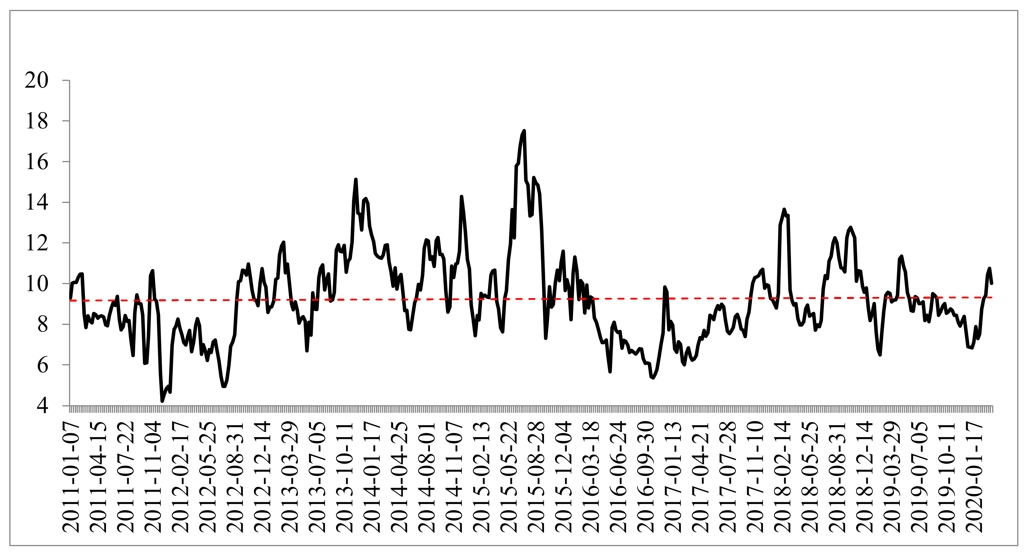
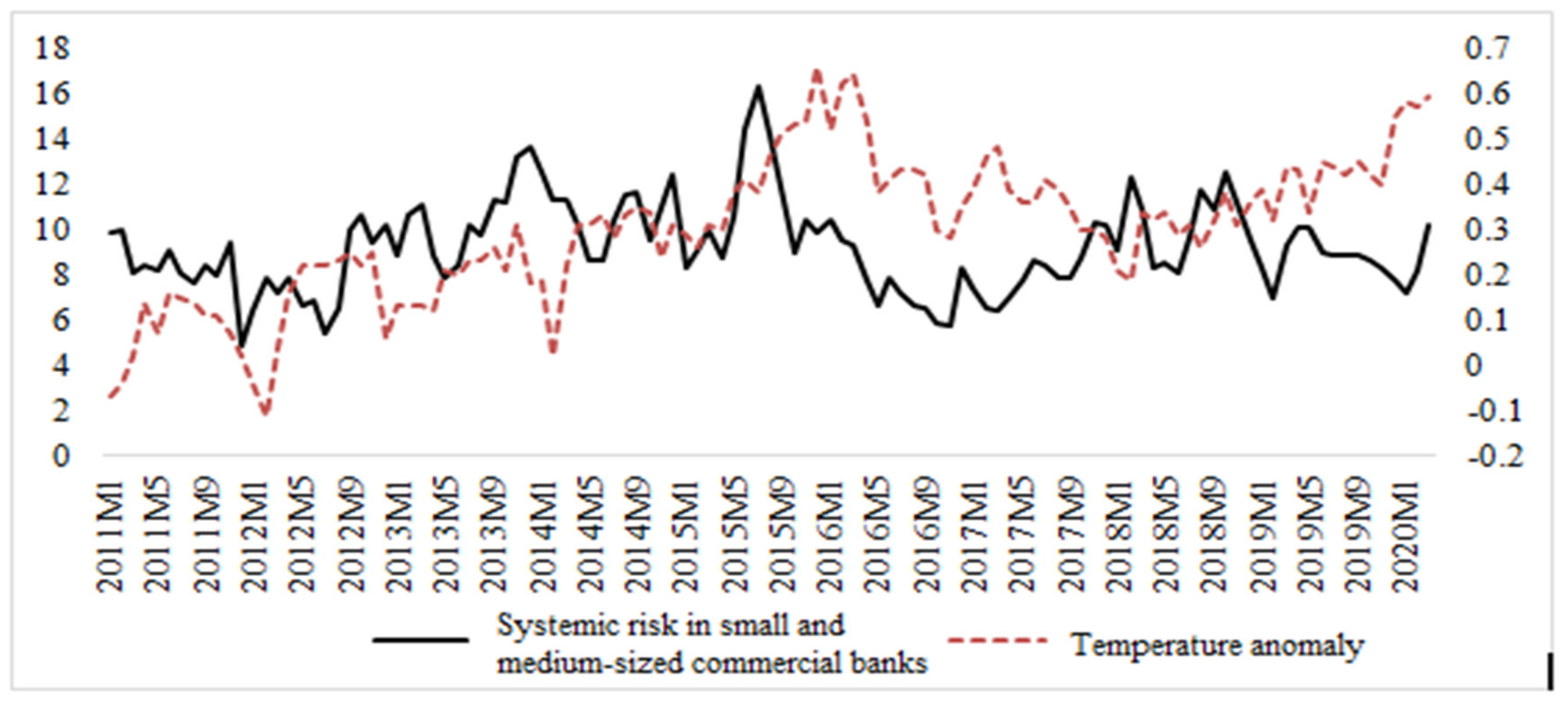
3.1.4. Empirical Results

The dynamic CoVaR value of each bank was measured according to the model, estimate 99% and 50% quantile regression models, calculate the dynamic systemic risk in the bank i, namely $\Delta {\mathrm{VaR}}_{0.99,\mathrm{t}}^{\mathrm{i}}$, [52].

Table 1. Estimated values of banks’ parameters when $q=99\%$

Banks	$\mathit{\beta }$	${\mathit{\gamma }}_1$	${\mathit{\gamma }}_2$	${\mathit{\gamma }}_3$	${\mathit{\gamma }}_4$	${\mathit{\gamma }}_5$	${\mathit{\gamma }}_6$
China Minsheng Bank	0.856345 (30.09)	0.2563	−0.1219	13.8702	0.6294	−3.4297	6.0078
Huaxia Bank	0.685290 (28.14)	8.0419	0.0316	8.3495	8.9260	0.8924	−7.2788
Bank of Beijing	0.765317 (25.08)	−0.1324	−0.4479	4.9239	0.2894	−2.1921	0.4153
Bank of Nanjing	0.650929 (10.06)	−0.9238	−0.1688	3.1751	−3.0075	−2.7424	−7.8969
Bank of Ningbo	0.711595 (11.14)	0.7706	−0.1713	3.9613	1.0962	−2.8082	−3.9274
Ping An Bank	0.668712 (29.18)	4.2248	0.1875	13.9360	−0.2058	−5.3534	6.6150
Shanghai Pudong Development Bank	0.723375 15.78)	1.1720	−0.3501	7.4879	−0.6822	−5.3691	13.1230
Industrial Bank	0.798520 (33.31)	5.5964	0.4517	11.5811	6.6687	−2.5132	0.5325
China Merchants Bank	0.757308 (30.24)	0.5868	−0.1320	3.7779	1.6247	0.5291	−5.9086
China CITIC Bank	0.810208 (20.67)	13.6422	0.1862	11.2629	13.2790	−1.5200	−11.3298
China Everbright Bank	0.774710 (28.55)	9.0757	0.1234	9.4735	7.5043	−1.8522	−6.7870

and

Table 2. Estimated values of banks’ parameters when q = 50%.

Banks	$\mathit{\beta }$	${\mathit{\gamma }}_1$	${\mathit{\gamma }}_2$	${\mathit{\gamma }}_3$	${\mathit{\gamma }}_4$	${\mathit{\gamma }}_5$	${\mathit{\gamma }}_6$
China Minsheng Bank	-	−1.1966	−0.0518	−1.0987	−0.9090	−0.3519	1.6229
Huaxia Bank	-	−0.7739	−0.1368	−1.1132	−0.2164	−0.1428	1.0374
Bank of Beijing	-	−0.7974	−0.1307	−0.7848	−0.7721	−0.2203	0.6553
Bank of Nanjing	-	−0.2471	−0.0778	−0.8082	−0.0720	−0.2023	0.4323
Bank of Ningbo	-	−1.2653	−0.1016	−1.2730	−1.1757	−0.3384	1.1455
Ping An Bank	-	−0.9791	−0.0801	−1.6228	−0.7318	−0.1281	0.9631
Shanghai Pudong Development Bank	-	−0.7994	−0.0929	−1.0020	−0.5843	−0.4944	0.8505
Industrial Bank	-	−1.0974	−0.1585	−1.3098	−0.8411	−0.4610	1.2712
China Merchants Bank	-	−1.0088	−0.1553	−1.1124	−0.7291	−0.3858	1.1022
China CITIC Bank	-	−0.9109	−0.0312	−1.0315	−0.6562	−0.5171	1.8194
China Everbright Bank	-	0.1697	−0.0970	−1.1801	0.3483	−0.1299	−0.7992

indicate the estimated result of coefficient of the status variables using quantile regression and the contribution β of small banks to the overall banking risk in the sample under the 99% quantile. From the statistics of t, β of all small banks in the sample was relatively significant. In particular, β of relatively large small- and medium-sized banks was higher, demonstrating that the spillover effect of systemic risk was stronger in larger-sized banks.

To give a more detailed description of the dynamic changes of the overall systemic risk in the 11 small- and medium-sized commercial banks, the dynamic systemic risks of the 11 banks from 2011 until now were weighted and averaged as per the market value, so as to represent the trends of dynamic changes in the overall systemic risk in listed small- and medium-sized commercial banks. As shown in Figure 1, it can be observed that the systemic risk in the banking sector was basically stable, and reached a record high amid the stock market crash from June to August 2015, more than six standard deviations from the average, when the financial market was experiencing violent fluctuations. In early 2020, the systemic risk in the banking sector rebounded significantly due to the impact of COVID-19, so banks should remain particularly vigilant about the increased systemic risk caused by disasters.

3.2. Measurement of Risk caused by Climate Change

Climatic conditions vary in different regions and countries, as do the types and impacts of extreme climate events. The representative Climate Extremes Index (CEI), for example, meets the actual conditions in the United States, but cannot be directly applied to other countries and regions. In line with China’s actual climate characteristics and the impacts of different types of extreme climate events, Ren Guoyu et al. from the China Meteorological Administration’s National Climate Center have explored and developed comprehensive climate change indexes suitable for China to represent the comprehensive trend of changes in climate conditions [59]. Given the availability of data, this paper represented the changes in temperature using temperature anomaly, thereby directly measuring the trend of climate change.

3.2.1. Selection of Indicators

This paper selected the difference between the daily mean temperature and the historical average of daily mean temperature to measure the trend of climate change.

$$\mathrm{DP}={\mathrm{T}}_{\mathrm{i}}-{\overline{\mathrm{T}}}_{\mathrm{i}}$$

(9)

In the formula, DP is the daily temperature anomaly, while ${\mathrm{T}}_{\mathrm{i}}$ and ${\overline{\mathrm{T}}}_{\mathrm{i}}$ are the daily temperature in China and the mean temperature of the ith day in the historical year in China.

3.2.2. Data Processing and Analysis

Regarding the availability of data, national temperature data were not available, in consideration of the availability of the data on the systemic risk and other control variables of domestic small- and medium-sized banks and the little difference between global climate change and the climate change in China, so the publicly available data on global temperature anomaly were selected. This paper collected data on global monthly mean temperature from January 2007 to March 2020. By taking the 30-year monthly mean temperature from 1981 to 2010 as the benchmark value, it measured the difference between the monthly mean temperature from 1 January 2011 to 31 March 2020, and the benchmark value as the temperature anomaly.

4. Assessment of the Impact of Climate Risk on Systemic Risk in Commercial Banks

4.1. Regression Model Based on the Single-Factor Impact of Climate

The weighted average value of the systemic risk in the above 11 small-and medium-sized commercial banks was taken as the overall systemic risk in these banks, and the weekly data were converted into monthly average data. The selected impact variable was the climate risk index, and the above data on temperature anomaly measured were used as the impact variable. The data selected were from January 2011 to March 2020. The results in Figure 2 suggest that the temperature anomaly (DP) and systemic risk in banks (COVAR) show a consistent trend and correlation to some extent. This study performed a more in-depth quantitative analysis of the data concerning temperature anomaly and systemic risk in banks.

The following model was built to research the single factor pair of climate change:

$$\Delta {\mathrm{CoVaR}}_t={\mathsf{\alpha }}_1{\mathrm{DP}}_t+{\mathsf{\epsilon }}_t$$

(10)

Wherein t means time, $\Delta {\mathrm{CoVaR}}_t$ the overall systemic risk in the sampled small-and medium-sized commercial banks, and ${\mathrm{DP}}_t$. the trend of climate change.

Data were standardized to unify its format and remove its heteroscedasticity. The analysis below is performed on the series of the logs of all variables. The stationarity test was performed on the series data on DP and $\Delta \mathrm{CoVaR}$. Besides, the optimal lag order was decided based on the Akaike information criterion (AIC), and it was 4 herein. According to the results in

Table 3. Results of stationarity tests on time series of variables.

Variable	Test Form	t-Statistics	10% Threshold	Prob *	Results
$\Delta \mathrm{CoVaR}$	(c,t,0)	−4.020948	−2.580908	0.0019	Smooth
DP	(c,t,0)	−2.629114	−2.580908	0.0902	Smooth

Note: * MacKinnon (1996) one-sided p-values.

, all the series passed the ADF stationarity tests at the significance level of 10%, so both $\Delta \mathrm{CoVaR}$ and DP series are stationary series, and there may be cointegration between $\Delta \mathrm{CoVaR}$ and DP, satisfying the prerequisites for applying the cointegration theory.

4.1.1. Creation of Inter-Series Cointegration

A regression equation was created, and its parameters were estimated by ordinary least squares (OLS). The results are shown in

Table 4. Regression estimation results.

	Coefficient	t-Statistics	p Value	R2	DW Value
Constant	9.0372	1.906523	0.0983	0.24	0.5234
Dp	0.6229	1.817289	0.0652

.

According to the results of the cointegration regression equation, the residual series of the equation was obtained by transformation, and a stationarity test was performed on the value of residual series. The optimal lag order was decided to be 1 according to the AIC. The results are shown in

Table 5. Stationarity test on residual series.

Residual	ADF Test Value	10% Threshold	Results
ε($\Delta \mathrm{CoVaR}$ −Dp)	−4.0391	−2.8879	Smooth

below.

The results indicate that the residual series passed the stationarity test on series at the significance level of 5%, proving a certain stable relationship between temperature anomaly and systemic risk in banks. To be specific, the estimated results of the cointegration regression equation indicate that the coefficient of Dp is positive, suggesting a certain consistency between the trend of changes in temperature anomaly and the systemic risk in banks during the sample period.

4.1.2. Error Correction Model

The error correction model (ECM) can reflect the relationship of short-run fluctuations and long-run equilibrium between variables, and the ECM results of the variables $\Delta \mathrm{CoVaR}$ and DP were obtained using OLS and presented in

Table 6. Error correction model (ECM) estimated results.

	Coefficient	t-Statistics	p Value	Adjustment to Long-Run Equilibrium
Constant	−0.0041	−2. 364135	0. 0196	0.2629
D(Dp)	0.8244	1.817289	0.0652
ECM(−1)	−0.2629	−0.481435	0.6450

.

In the above ECM, the difference revealed the impact of short-run fluctuations. The fluctuations in the systemic risk in banks can be divided into two parts. First, the impact of systemic risk itself and the short-run fluctuations in temperature anomaly. The short-run impact is relative to the aforesaid long-run impact, which mirrored the overall trend from January 2011 to March 2020, while the short-run impact here refers to the fluctuations in the past few years. According to the coefficient of short-run D(Dp), the short-run impact of temperature anomaly on systemic risk in the banking sector was positive, illustrating that like long-run impact, it was generally a factor in the growth of systemic risk. This positive effect was small, but slightly greater than that of the long-run impact. The aforesaid results demonstrate that, for a shorter period, climate warming worsened risks in banking to a certain degree.

Second, the impact of deviation from long-run equilibrium. The coefficients in ECM indicated the adjustment of temperature to the deviation of systemic risk from long-run equilibrium. It can be observed that the coefficient was relatively small, so the capability of temperature to correct such deviation is almost negligible. The direct impact of temperature on systemic risk in banks is insignificant because such risk is attributable to a variety of factors.

4.2. Building a Regression Model of Multiple-Factor Impact

In actual financial activities, banks’ own financial characteristics are also an important factor influencing their systemic risk, but the financial characteristics and systemic risk are both disturbed by climate factors. This paper, therefore, considered including such characteristics in the model as a mediator variable for a more rounded assessment of the contribution of dynamic influencing factors of systemic risk in banks.

4.2.1. Research Hypothesis

(1) Business structure. The deterioration of climate change risks impacts banks in the following ways. On the one hand, natural disasters resulting from climate change will impact private saving, thus undermining the banks’ foundation for liabilities. On the other hand, they will affect the banks’ asset business, driving down the size and quality of loans offered by commercial banks. In this paper, the loan-deposit ratio (LDR), i.e., the ratio of a commercial bank’s total loans to its total savings, was selected to measure the changes caused by climate risk to the banks’ asset/liability business. A lower loan-deposit ratio implies the banks’ poorer utilization efficiency of assets and lower profitability.

On the basis of the above analysis, H1 was proposed, namely that the risk from climate change would reduce the loan-deposit ratio of commercial banks and increase the systemic risk in the banking sector.

(2) Asset quality. Loans are the most important asset type of banking and financial institutions, so the primary impact of climate change on banks’ asset quality is its impact on the credit quality of loan portfolios. UNEP revealed in its 2006 report that the potential exposure of risk from climate change was high in such industries as coal, petroleum, power, cement, and aluminum, which were exposed to severe policy supervision and input price risk. These industries would adversely impact the banks’ asset quality once they were exposed to the risk from climate change because of policies for industrial transition. The NPL ratio is the principal indicator for measuring the asset quality of commercial banks, so an increased NPL ratio suggests deterioration in asset quality and increase in systemic risk in the banking sector.

On the basis of the above analysis, H2 was proposed, namely that climate change risks would increase the loan-deposit ratio of commercial banks and the systemic risk in the banking sector.

(3) Profit margin. Climate change will decrease the profits of commercial banks. The profits of commercial banks in China are mostly derived from debit and credit spreads, so this paper employed NIM to measure the profitability of commercial banks in China. The narrower NIM of commercial banks suggests increased systemic risk in the banking sector.

On the basis of the above analysis, this paper put forward H3, namely that climate risk would narrow the NIM of commercial banks and push up the systemic risk in the banking sector.

4.2.2. Model Building

(1) Sample selection and data sources

The impact of climate change on systemic risk is one-way only, so regarding the model selection, the least squares regression was adopted to assess the multiple regression model. The following model was built herein to analyze the impact of climate change on systemic risk in the small- and medium-sized banks in the sample:

$$\Delta {\mathrm{CoVaR}}_t={\mathsf{\alpha }}_1{\mathrm{DP}}_t+{\mathsf{\alpha }}_2{\mathrm{Mediator}}_t+{\mathsf{\epsilon }}_t$$

(11)

Wherein t means time, $\Delta {\mathrm{CoVaR}}_t$ the overall systemic risk in the sample small-and medium-sized commercial banks, ${\mathrm{DP}}_t$ the trend of climate change, and Mediator_t other mediator variables.

(2) Setting of variables

Dependent variable: The weighted average value of the systemic risk in the above 11 small- and medium-sized commercial banks was taken as the overall systemic risk in these banks ($\Delta \mathrm{CoVaR}$), and the weekly data were converted into monthly average data, which were standardized to remove the impact of negative values. The greater $\Delta \mathrm{CoVaR}$ suggests higher systemic risk in a bank.

Independent variable: The data on temperature anomaly (DP) measured in Part III were used as the independent variable to represent the factors of climate change.

Mediator variables: Based on the above analysis, this paper maintains that climate change may influence the systemic risk in China’s banks by affecting the business structure, asset quality, and profit margin of commercial banks. The loan-deposit ratio (LDR) of commercial banks was taken as a measurement indicator for business structure; NPL ratio as a measurement indicator for asset quality; and NIM as a measurement indicator for changes in profit margin. The quarterly data on these three variables were converted into monthly data.

The data period was from January 2011 to March 2020, with a view to ensuring consistency in the length of bank data and avoiding the impact of the 2007 sub-prime mortgage crisis. The operating data on these banks were sourced from their reports, and the macroeconomic data from the Wind databases. The weekly and quarterly data were converted into monthly data for analysis. Data were processed using the statistical software Eviews.

4.2.3. Empirical Research and Result Analysis

(1) Descriptive statistics

Table 7. Results of descriptive statistics about variables.

	$\mathbf{\Delta }\mathbf{CoVaR}$	DP	LDR	NPL	NIM
Mean	9.2247	0.3010	0.7948	0.0122	0.0243
Median	8.8760	0.3100	0.7432	0.0141	0.0251
Maximum	16.3015	0.6600	0.9607	0.0173	0.0290
Minimum	4.8304	−0.1100	0.6757	0.0055	0.0192
Std. Dev.	1.9991	0.1579	0.0944	0.0044	0.0029
Skewness	0.6383	−0.1895	0.5480	−0.3365	−0.1970
Kurtosis	3.8311	2.9433	1.6649	1.4049	1.6743
Observations	111	111	111	111	111

sets out the results of descriptive statistics about the dependent variable, independent variable, mediator variables, and control variable.

As indicated by the statistical results, from 2011 to the beginning of 2020, the standard deviation of $\Delta \mathrm{CoVaR}$ regarding systemic risk in China’s small- and medium-sized commercial banks was 1.9991, and the difference between the minimum and maximum values surpassed 10, demonstrating sharp fluctuations in the overall risk profile of these banks during the sample period. Additionally, the average value of temperature anomaly was 0.30, in line with the trend of climate warming. The standard deviation of LDR was greater among the three mediator variables, illustrating dramatic changes in the business structure of small- and medium-sized commercial banks during the sample period. By contrast, that of the NPL ratio was small, suggesting that the asset quality of China’s commercial banks was relatively stable and within a reasonable range.

(2) Stationarity test

Before building a regression model, this paper conducted separate ADF tests on the dependent variable, independent variable, and three mediator variables, so as to prevent spurious regression. Specifically, at the 5% confidence level, $\Delta \mathrm{CoVaR}$ of the overall systemic risk in small- and medium-sized banks was stationary in the original series; climate change DP, LDR, NIM, and NPL ratio became stationary after the first order differentiation. The test results suggest that the orders of integration of more than two variables in the dependent variable exceeded those of the independent variable and were the same, so a cointegration relationship can be established. Test results are shown in

Table 8. Results of stationarity tests on time series of variables.

Variable	Test Form	t-Statistics	10% Threshold	Prob *	Results
$\Delta \mathrm{CoVaR}$	(c,t,0)	−4.0048	−4.0436	0.0112	Smooth
DP	(c,0,0)	−2.6291	−2.8879	0.0902	Not smooth
D(DP)	(c,0,0)	−12.4167	−2.8882	0.0000	Smooth
LDR	(c,t,1)	−2.2407	−3.4516	0.4622	Not smooth
D(LDR)	(c,t,2)	−7.8801	−3.4523	0.0000	Smooth
NPL	(c,0,1)	−1.5993	−2.8882	0.4795	Not smooth
D(NPL)	(c,0,0)	−3.2312	−2.8882	0.0208	Smooth
NIM	(c,0,1)	−1.7209	−2.8882	0.4180	Not smooth
D(NIM)	(c,0,2)	−21.4569	−2.8887	0.0000	Smooth

Note: * MacKinnon (1996) one-sided p-values.

:

(3) Cointegration test

Johansen’s test was selected to test whether there was a long-run and stationary equilibrium between variables. The results of the VAR model indicated that the optimal lag order was 2, so the maximum lag order used in Johansen’s test was 1. The results of the trace test and maximum eigenvalue test are shown in

Table 9. Result of Johansen’s test for cointegration.

Null Hypothesis	Trace Test			Null Hypothesis	Maximum Eigenvalue Test
	Statistics	Threshold (5%)	p Value		Statistics	Threshold (5%)	p Value
None *	111.2557	95.7537	0.0028	None *	41.3392	40.0776	0.0358
At most 1 *	69.9165	69.8189	0.0491	At most 1	25.2442	33.8769	0.3687
At most 2	44.6723	47.8561	0.0966	At most 2	19.2678	27.5843	0.3941
At most 3	25.4045	29.7971	0.1475	At most 3	14.3335	21.1316	0.3383
At most 4	11.071	15.4947	0.2072	At most 4	9.2030	14.2646	0.2697
At most 5	1.8680	3.8415	0.1717	At most 5	1.8680	3.8415	0.1717

Note: * denotes rejection of the hypothesis at the 0.05 level.

below. It can be observed that there was at most one cointegration equation between variables, so there was a long-run and dynamic equilibrium relationship between them.

(4) Multiple collinearity test

This paper first tested whether there was multicollinearity to ensure the estimated results were unbiased before the least squares regression was employed.

VIF (variance inflation factor) is one of the methods to detect multicollinearity. As the reciprocal of tolerance, VIF is positively correlated with collinearity. In case of multiple variables, if VIF falls between 0 and 10, this proves no multicollinearity between variables. Results of the multiple collinearity test are shown below in

Table 10. Multiple collinearity test.

Variable	DP	LDR	NPL	NIM
R2	0.641	0.748	0.867	0.812
VIF	2.788	3.964	7.528	5.309

:

(5) Model estimation and analysis

① Model estimation of the impact of climate change on the overall systemic risk in banks

It can be concluded from the above that there was a weak linear positive correlation between the temperature anomaly and the overall systemic risk in small-and medium-sized commercial banks, so the model set herein is as follows:

$$\Delta {\mathrm{CoVaR}}_{\mathrm{t}}={\mathsf{\alpha }}_1{\mathrm{DP}}_{\mathrm{t}}+{\mathsf{\alpha }}_2{\mathrm{LDR}}_{\mathrm{t}}+{\mathsf{\alpha }}_3{\mathrm{NPL}}_{\mathrm{t}}+{\mathsf{\alpha }}_4{\mathrm{NIM}}_{\mathrm{t}}+{\mathsf{\epsilon }}_{\mathrm{t}}$$

(12)

The model estimation results are in

Table 11. Model estimation results (OLS).

Variable	Coefficient	Standard Deviation	t-Statistics	p Value
DP	0.7274	2.0160	0.3608	0.7190
LDR	−6.5623	4.0210	−1.6320	0.1056
NIM	−23.7898	152.5949	−0.1559	0.8764
NPL	76.5610	118.2888	0.6472	0.5189
ε	13.8658	6.2878	2.2052	0.0296
R-squared	0.0363	Mean dependent var		9.2247
Adjusted R-squared	−0.0001	S.D. dependent var		1.9991
S.E. of regression	1.9992	Akaike info criterion		4.2674
Sum squared resid	423.6586	Schwarz criterion		4.3894
Log likelihood	−231.8388	Hannan-Quinn criter.		4.3169
F-statistic	0.9970	Durbin-Watson stat		0.5451
Prob(F-statistic)	0.4126

as follows.

According to the significance test and Table 11, except for the constant term that was significant at the 5% significance level, other parameters were not significant, nor was the overall linearity test of the regression model. The model was therefore likely to have heteroscedasticity. The Breusch–Pagan test was used to test heteroscedasticity in the model. Significance was determined through Obs*R-square statistic or the corresponding p-value in

Table 12. Heteroscedasticity test.

F-Statistics	Prob.F	obs*R-Square	Prob.chi-Square
3.792163	0.0064	13.89568	0.0076

, and it was found that p-value = 0.0076 and that the null hypothesis was rejected, so heteroscedasticity existed in the model.

It can be seen from the above that the existence of heteroscedasticity in the model was revealed by the test, so to guarantee the sound statistical properties of the regression parameter estimates, the development of novel methods for model estimation to remove heteroscedasticity was necessary. The most commonly used method is the weighted least squares. Using weighted least squares (WLS), the original model is weighted so that it can become a new model without heteroscedasticity, and then the ordinary least squares method (OLS) is employed to estimate the model’s parameters. By taking the reciprocal 1/abs($e_t$) in the residual estimator series $e_t$ of the original model as the weight, the new model is as follows:

$$\frac{1}{\left|e_t\right|}\Delta \mathrm{Co}{\widehat{\mathrm{VaR}}}_{\mathrm{t}}=\widehat{{\mathsf{\alpha }}_1}\frac{1}{\left|e_t\right|}{\mathrm{DP}}_{\mathrm{t}}+\widehat{{\mathsf{\alpha }}_2}\frac{1}{\left|e_t\right|}{\mathrm{LDR}}_{\mathrm{t}}+\widehat{{\mathsf{\alpha }}_3}\frac{1}{\left|e_t\right|}{\mathrm{NPL}}_{\mathrm{t}}+\widehat{{\mathsf{\alpha }}_4}\frac{1}{\left|e_t\right|}{\mathrm{NIM}}_{\mathrm{t}}+\frac{1}{\left|e_t\right|}\widehat{{\mathsf{\epsilon }}_{\mathrm{t}}}$$

(13)

This model was estimated by Eviews, and the estimation results are in

Table 13. Model estimation results (WLS).

Variable	Coefficient	Standard Deviation	t-Statistics	p Value
ε	13.3045	1.687277	7.885192	0.0000
DP	0.9027	0.417235	2.163685	0.0327
LDR	−5.6124	0.680173	−8.251482	0.0000
NIM	−23.7731	47.19046	−0.503770	0.6155
NPL	55.0378	31.47661	1.748531	0.0833
Weighted Statistics
R-squared	0.7710	Mean dependent var		9.1596
AdjustedR-squared	0.7623	S.D. dependent var		18.6795
S.E. of regression	0.5254	Akaike info criterion		1.5950
Sum squared resid	29.2712	Schwarz criterion		1.7170
Log likelihood	−83.5248	Hannan-Quinn criter.		1.6445
F-statistic	89.2337	Durbin-Watson stat		0.9686
Prob(F-statistic)	0.0000	Weighted mean dep.		9.2538
Unweighted Statistics
R-squared	0.0355	Mean dependent var		9.2247
Adjusted R-squared	−0.0009	S.D. dependent var		1.9991
S.E. of regression	1.9999	Sum squared resid		423.9786
Durbin-Watson stat	0.5442

as follows.

It is found in Table 13 that after WLS, the test of parameter T, except for NIM, was significant, R-squared dramatically increased, and that F test was also significant.

The regression model is obtained:

$$\Delta \mathrm{Co}{\widehat{\mathrm{VaR}}}_{\mathrm{t}}=13.3045+0.9027\mathrm{DP}-5.6124\mathrm{LDR}-23.7731\mathrm{NIM}+55.0378\mathrm{NPL}$$

(14)

Table 13 indicates the results of multiple regression analysis for the total effect of climate change on systemic risk in banks. The adjusted R²value of the model was 0.7623, and F statistic was 89.2337 and it passed the test at the 1% significance level. This suggested that the overall goodness of fit of the model was satisfactory.

Regarding the mediator variables, NPL ratio and LDR were significant at the 1% confidence level. Additionally, the coefficient of NPL ratio was positive, implying that the increase in NPL ratio would accelerate the spread of systemic risk in banks during the sample period. The coefficient of NIM was negative, suggesting that narrowed NIM would contribute to increased systemic risk in banks during the sample period. As an important indicator for measuring the liquidity of a bank, an increase in LDR means a decrease in liquidity, and the systemic risk in the banking sector should go up. In the above model estimation, nevertheless, the coefficient of LDR was negative, so LDR was inversely correlated with systemic risk in the banking sector. The increase in LDR indicated the increase in the banks’ utilization efficiency of capital and profitability, suggesting that the increased LDR within a certain interval implied improved operating capability, thereby lowering the operational risk.

The regression coefficient between the independent variable, temperature anomaly (DP), and systemic risk in banks ($\Delta \mathrm{CoVaR}$), was 0.9028, and was significant at the 1% confidence level. This demonstrated that the rise in temperature factor exacerbated the overall systemic risk in banks during the sample period, but such exacerbation was mild. Although this conclusion is in consistence with the idea that risk from climate change will exacerbate financial risks in banks, the following two facts must be taken into account. First, the contributors to systemic risk in banks are complex, and concern the macroeconomic environment, banks’ operating status, as well as market liquidity. The risk from climate change affects systemic risk in banks by influencing a variety of economic and environmental factors, rather than exercising a direct impact on such risk. Second, the length of the sample data may cause climatic factors to deviate from systemic risk in banks, since the considerable harm caused by climate change tends to become apparent only over a long period of time. Next, this paper will put into consideration how climate change affects the systemic risk in banks by influencing other factors related to such risk.

② Empirical analysis of the impact of climate change on mediator variables

An estimation test of the effect of climate change on mediator variables was performed using least squares regression, and the test results were in

Table 14. Test results of climate change on mediator variables.

Variable	Mediator Variable
	LDR	NPL	NIM
DP	0.8245 ***	26.9530 ***	−26.6535 ***
Constant term	−0.3543 ***	−0.0276	0.9484 ***

Note: *** significant at p < 0.01.

as follows:

As can be observed from Table 14, the impact of climate change on NPL ratio and LDR was significantly positive, suggesting that the LDR and NPL ratio of small- and medium-sized commercial banks increased as the temperature anomaly grew during the sample period. The temperature anomaly had a greater impact on NPL ratio than on the other two indicators. The anomaly was negatively correlated with NIM, demonstrating that climate change would decrease NIM and thus the banks’ profitability over the sample period.

③ Test for mediation effect based on the Bootstrap method

According to the above analysis, a possible mediation effect between the dependent variable and independent variable was identified, meaning that the independent variable affected the dependent variable via mediator variables. Next, this paper employed the PROCESS macro for SPSS, and discussed how the independent variable affected the dependent variable based on the Bootstrap method. Since the aforesaid test of model found that heteroscedasticity existed in the dependent variable, independent variable, and mediator variables, the series of variables was weighted by the above estimated weight to test mediation effect.

Table 15. Test for mediation effect based on bootstrap method.

Impact Path	Direct and Indirect Effect	BootSE	Interval Floor	Interval Ceiling
DP→$\Delta \mathrm{CoVaR}$	−0.7776	0.5005	−1.7698	0.2146
DP→LDR→$\Delta \mathrm{CoVaR}$	−3.1010	2.8845	−9.0448	3.2072
DP→NPL→$\Delta \mathrm{CoVaR}$	5.9292	2.0357	1.6650	10.0711
DP→NIM→$\Delta \mathrm{CoVaR}$	16.7177	7.4589	11.3047	38.6391

uses the Bootstrap method to test the impact of climate change on systemic risk in the banking sector through the three mediator variables.

It can be found from

Table 16. Summary of hypothesis testing results.

Hypothesis	Hypothesis Details	Results
H1	Climate change would reduce the LDR of commercial banks and increase the systemic risk in the banking sector.	Not supported
H2	Climate change would increase the NPL ratio of commercial banks and the systemic risk in the banking sector.	Supported
H3	Climate change would narrow the NIM of commercial banks and increase the systemic risk in the banking sector.	Not supported

that the upper and lower limits for the temperature factor affecting systemic risk in banks included 0, suggesting that the direct impact of this factor on the systemic risk in banks was not significant. The upper and lower limits for climate change affecting systemic risk in banks via NPL ratio and NIM excluded 0, indicating that climate change significantly affected the systemic risk in banks by affecting the NPL ratio and NIM of commercial banks, with significant indirect effects. The mediation effect of the NPL ratio was positive, demonstrating that the increase in temperature factor would raise the NPL ratio of commercial banks, thus pushing up their systemic risk. Additionally, the mediation effect of NIM was positive, implying that the increase in temperature factor did not lower the systemic risk concurrently with the growth of NIM. This is indirect proof that the temperature factor cannot exacerbate systemic risk by reducing the mediation effect of NIM. The upper and lower limits for the temperature factor affecting systemic risk in banks through LDR included 0, illustrating that the indirect impact of this factor on systemic risk in banks through LDR was not significant.

The goodness of fit of the aforesaid models indicate that climate change was positively correlated with the overall systemic risk in the sample commercial banks, while the increase in NPL ratio and NIM would respectively increase and decrease the systemic risk, consistent with general experience. The results of the mediation test prove that climate change significantly affected the overall systemic risk in the sample commercial banks through the NPL ratio, meaning that the increase in temperature anomaly would boost the NPL ratio, thereby exacerbating the overall systemic risk in commercial banks.

5. Discussion

5.1. The Main Innovation of This Study

The impact of climate change on systemic risk is yet to be revealed, and its impact on the entire financial market is minor at present. As the climate and environment deteriorate, however, climate change will pose a serious risk to the risk exposure of the banking sector in the long run. Currently, commercial banks in China have started paying attention to green loans, but lack assessment of the climate adaptability of loan business. The gap of financial supervision in climate adaptability of loan assets substantially enhances the probability of exposure of the banking sector to the risk from climate change in the future. In comparison with the existing relevant studies, the research process and conclusions of this study are innovative. Few existing studies involved the relationship between climate change and systemic risk of the banking industry. For example, Battiston S. et al. (2017) analyzed the impact of climate policy on the financial system. Their independent and dependent variables were different from those in this study [1]; so was their research method. Although Giusy C et al. (2020) adopted the same method as this study, the content of the study was different from that of this study [3]. On the basis of review of the existing literature, the research topic, mechanism, and process of this study show great innovation.

(1) This study analyzed the tendency of climate and systemic risk within a long period, through the regression model with the single factor, climate. The analysis result demonstrated that the changes in both factors are generally relevant, which was a qualitative understanding of their relationship. Furthermore, the single-factor regression model was employed to prove the quantitative relevance between the two factors. The research process not only abandoned the shortcoming of simple demonstration methods of qualitative research of the existing studies (e.g., Battiston S., 2017; Lei Yao & Zhao Tianyi, 2019); Sun Tianyin, 2020; Tan Lin & Gao Jialin, 2020), but also effectively proved the impact of climate change on systemic risk of banks [1,25,26,27].

(2) The single-factor regression model might omit some important impact factors of systemic risk. Hence, this paper adopted a multi-factor regression model to deepen the understanding of the comprehensive factors of systemic risk. Moreover, it probed into the mechanism of action between them. This paper discovered the mediating effect of NPL ratio and loan-to-deposit ratio on the influence of climate change on systemic risk, which broke the stereotype research on climate and risk. Furthermore, this paper explored the mechanism of the impact of climate change on systemic risk. Therefore, banks and government regulators can formulate effective climate-finance policies by referring to the research results of this study. Besides, banks can effectively predict systemic risk arising from climate change.

5.2. Countermeasure Suggestions for Banks and Government

Based on the validity of the research conclusions, this paper puts forward suggestions from two aspects, namely banks and government regulators.

(1) Suggestions for banks. In accordance with the aforesaid argument, climate change can significantly affect systemic risk of banks. In view of this, banks can adopt the following measures to prevent risks. First, commercial banks should take climate change as a strategic issue, and senior management should improve their awareness of risk from climate change. Besides, banks should step up the identification and information disclosure concerning climate change risks and opportunities, and allocate resources to support green transition and development. Second, banks should establish a complete management system for environmental and social risk, incorporate climate adaptability into their lending decisions, perfect their internal policies for management over climate risk regarding business, and carry out dynamic management of climate risk. Third, banks should develop quantitative risk management and credit assessment instruments for analysis of the impact of climate change and perform scenario analysis of climate risk and climate adaptability as well as climate stress tests [53].

(2) Government monitoring. Regarding government regulation, climate change is the consequence of multiple factors. Governments, as the rule-maker and executor, should carry out mandatory supervision, guiding the public and enterprises to make long-term and holistic strategic planning during top-level design. As it is impossible to curb climate change, governments can only realize sustainable development via effective guidance. Moreover, banks and governments should join hands to prevent possible systemic risk. Therefore, this paper gives the following suggestions for government regulation. First, the issue of climate change should be included in the macroprudential framework. Also, financial stability assessment should be conducted. The factor of climate change should be incorporated into the existing macroprudential framework. The risk to financial stability posed by climate change should be assessed. At present, Chinese regulators have not attached sufficient importance to the systemic financial risks that may result from climate change. Given the Chinese economy’s heavy reliance on traditional energies and production modes and the large size of the existing loans granted by banks to traditional energy companies, it is necessary to build an assessment model for financial stability that takes global climate change into account and will give early warnings about related risks to financial institutions. Second, unified criteria for assessment and grading of projects’ climate adaptability and mitigation should be established for the banking sector. Such criteria should be an important part of the due diligence process prior to loan extensions in the banking sector. Third, a compensatory mechanism for climate risk should be created for inclusive credit projects regarding industries vulnerable to climate change that concern national interest and people’s livelihood, including agriculture, forestry, animal husbandry and fishery, mining, tourism, retail, and wholesale. Such a mechanism would minimize the risks associated with bank loans for industries vulnerable to climate change, while helping to enhance the climate adaptability of these industries. Fourth, financial support for the advancement of new energy, clean energy, and green low-carbon industries should be stepped up, so as to facilitate the transition to a low-carbon economy. Additionally, the impact of climate change should be reduced and mitigated through support for the development of green industries.

6. Conclusions

This paper explored the influence of climate change on systemic risk of banks, based on the monthly data for 2011 to 2020 on 11 listed small- and medium-sized commercial banks in China. The relevant conclusions are below:

(1) The empirical test based on the regression model with the single factor of climate revealed that temperature departure and systemic risk of banks are correlated, to some extent. In addition, the stationary test discovered that there is a stable relation between temperature departure and systemic risk of banks. In other words, changes in temperature departure are consistent with those in systemic risk of banks. In the short run, climate warming aggravates systemic risk of banks, to some extent. In the long run, systemic risk of banks is derived from multiple factors. The influence of the single factor, air temperature, can only exert a limited impact on systemic risk of banks. Thus, a multi-factor model should be developed to gain deeper insight into the comprehensive influence on systemic risk of banks.

(2) This paper, based on its multi-factor model, revealed that: First, climate change plays a positive but minor role in systemic risk in banks in the long run. In addition, the adjustment of climate change to the long-run deviation of systemic risk is slight. Also, the capability of temperature to correct the long-run equilibrium of systemic risk is almost negligible. This suggests that a wide range of factors contribute to systemic risk in banks, and that in the short run, climate factor is one of the less significant factors. Second, the empirical results of the mediation effect imply that, over the sample period, the increase in NPL ratio significantly exacerbated the spread of systemic risk in banks, and narrowed NIM would significantly push up such risk. There is a positive correlation between climate change and systemic risk in banks within the confidence interval. Third, the test results of the mediation effect on variables refuted the hypotheses that climate change affects systemic risk in banks through NIM and LDR, but supported the hypothesis that climate change affects systemic risk in banks through the NPL ratio. The indirect effect of climate change on systemic risk in banks through the NPL ratio is significantly positive, meaning that climate warming has pushed up the NPL ratio and therefore increased the banks’ systemic risk.

Certainly, this study still has limitations due to some objective reasons. Such limitations are mainly found in the measurement of climate change. Data on global abnormal temperature were employed to measure climate change in China. There are some errors in terms of the matching of the existing data on climate change with the data on the dependent variable, systemic risk, attributable to data availability. This study would be optimized and deepened through more perfectly matched data to be found by these authors or readers. Nevertheless, this study is of theoretical and practical significance with respect to the prediction of systemic risk of banks from the viewpoint of climate change. Additionally, its research on the relevant mechanism of action is innovative and inspiring.

References

1. Battiston, S.; Mandel, A.; Monasterolo, I.; Schütze, F.; Visentin, G. A climate stress-test of the financial system. Nat. Clim. Chang. 2017, 7, 283–288. [Google Scholar] [CrossRef]
2. Huntington, E.; Visher, S.S. Climatic Change: Their Nature and Causes; Yale University Press: New Haven, CO, USA, 1922; p. 2. Available online: https://www.questia.com/library/94928129/climatic-changes-their-nature-and-causes (accessed on 17 November 2020).
3. Giusy, C.; Gianfranco, G.; Marco, S. Climate change and credit risk. J. Clean. Prod. 2020, 266, 1–10. [Google Scholar]
4. Agassiz, L. Tudes Sur Les Glaciers; Privately Published; Neuch Tel: Paris, France, 1840. [Google Scholar]
5. Hay, W.W.; Robert, M.D.; Christopher, N.W. The Late Cenozoic up lift climate change paradox. Int. J. Earth Sci. 2002, 91, 746–774. [Google Scholar] [CrossRef] [Green Version]
6. Bernanke, B. A Letter to Sen. Bob Corke. Wall Str. J. 2009, 11, 18. [Google Scholar]
7. Kaufman, G.G.; Kenneth, E.S. What Is Systemic Risk, and Do Bank Regulators Retard or Contribute to It? In The Independent Review; The Independent Institute: Oakland, CA, USA, 2003; pp. 371–391. Available online: https://law.stanford.edu/publications/what-is-systemic-risk-and-do-bank-regulators-retard-or-contribute-to-it/ (accessed on 17 November 2020).
8. Dansgaard, W.; Johnsen, S.J.; Clausen, H.B.; Dahl-Jensen, D.; Gundestrup, N.S.; Hammer, C.U.; Hvidberg, C.S.; Steffensen, J.P.; Sveinbjörnsdottir, A.E.; Jouzel, J. Evidence for general instability of past climate from a 250 kyr ice core record. Nature 1993, 364, 218–220. [Google Scholar] [CrossRef]
9. De Bandt, O.; Hattmann, P. Systemic Risk A Survey. Available online: https://papers.ssrn.com/sol3/papers.cfm?abstract_id=258430 (accessed on 17 November 2020).
10. Huntington, E. Climatic Variations and Economic Cycles, Geographical Review; Taylor & Francis, Ltd.: New York, NY, USA, 1916. [Google Scholar]
11. Smaga, P. The Concept of Systemic Risk. Available online: https://papers.ssrn.com/sol3/papers.cfm?abstract_id=2477928 (accessed on 17 November 2020).
12. Szpunar, P.J. Rola polityki makroostrożnościowej w zapobieganiu kryzysom finansowym. Narodowy Bank Polski. Departament Edukacji i Wydawnictw. 2012, 278. [Google Scholar] [CrossRef]
13. Adrian, T.; Brunnermeier, M.K. CoVaR. Am. Econ. Rev. 2006, 106, 1705–1741. [Google Scholar] [CrossRef]
14. Acharya, V.; Pedersen, L.; Philippon, T.; Richardson, M. Measuring Systemic Risk. Rev. Financ. Stud. 2017, 30, 2–47. [Google Scholar] [CrossRef]
15. Brownlees, C.; Engle, R.F. SRISK: A Conditional Capital Shortfall Measure of Systemic Risk. Rev. Financ. Stud. 2017, 30, 48–79. [Google Scholar] [CrossRef]
16. Aglietta, M.; Espagne, E. Climate and Finance Systemic Risks, more than an Analogy? The Climate Fragility Hypothesis. Available online: https://www.researchgate.net/profile/Etienne_Espagne/publication/305307236_Climate_and_Finance_Systemic_Risks_more_than_an_analogy_The_climate_fragility_hypothesis/links/57876ef808aea8b0f0c2bcd3.pdf (accessed on 7 November 2020).
17. Batten, S.; Sowerbutts, R.; Tanaka, M. Let’s Talk About the Weather: The Impact of Climate Change on Central Banks. Available online: https://papers.ssrn.com/sol3/papers.cfm?abstract_id=2783753 (accessed on 7 November 2020).
18. Dafermos, Y.; Nikolaidib, M.; Galanisc, G. Climate Change, Financial Stability and Monetary Policy. Ecol. Econ. 2018, 152, 219–234. [Google Scholar] [CrossRef]
19. Bank of England. The impact of climate change on the UK insurance sector: A climate change adaptation report by the Prudential Regulation Authority. Available online: https://www.bankofengland.co.uk/-/media/boe/files/prudential-regulation/publication/impact-of-climate-change-on-the-uk-insurance-sector.pdf (accessed on 7 November 2020).
20. FSB. Recommendations of the Task Force on Climate-related Financial Disclosures. June, 2017 [N/OL]. Available online: https://www.fsb-tcfd.org/wp-content/uploads/2017/06/FINAL-TCFD-Report-062817.pdf (accessed on 6 June 2019).
21. Center for American Progress, Climate Change Threatens the Stability of the Financial System by Gregg Gelzinis and Graham Steele 2019. Available online: https://www.americanprogress.org/issues/economy/reports/2019/11/21/477190/climate-change-threatens-stability-financial-system/ (accessed on 21 November 2019).
22. European Central Bank. The Financial Stability Review. Frankfurt, 2019. Available online: https://www.ecb.europa.eu/pub/financialstability/fsr/html/ecb.fsr201905~266e856634.en.html#toc1 (accessed on 16 March 2019).
23. Economist Intelligence Unit. The Cost of Inaction: Recognising the Value at Risk from Climate; Chane: London, UK, 2015. [Google Scholar]
24. Dowla, A. Climate Change and Microfinance. Bus. Strat. Dev. 2018. [Google Scholar] [CrossRef]
25. Yao, L.; Tianyi, Z. Managing Financial Risks from Climate Change. Available online: https://www.citivelocity.com/citigps/managing-financial-risks-climate-change/ (accessed on 17 November 2020).
26. Tianyin, S. Analysis on Sustainable Finance and Climate Risk. Financ. Perspect. J. 2020, 2, 24–31. [Google Scholar]
27. Lin, T.; Jialin, G. Research on the Mechanism and Countermeasures of the Financial System for Risk from Climate Change. J. Financ. Dev. Res. 2020, 1, 13–20. [Google Scholar]
28. Qiang, Z.; Han, Y.; Song, L. The Summary of Development in Global Climate Change and Its Influencing Factors. Adv. Earth Sci. 2005, 20, 47–60. [Google Scholar]
29. Qin, D.H.; Chen, Z.L.; Luo, Y.; Ding, Y.H.; Dai, X.S.; Ren, J.W.; Zhai, P.M.; Zhang, X.Y.; Zhao, Z.C.; Zhang, D.E. Updated Understanding of Climate Change Sciences. Adv. Clim. Chang. Res. 2007, 3, 63–73. [Google Scholar]
30. The National Climate Change Coordinating Group under the National Development and Reform Commission. Impacts of and Adaptation to Climate Change. In Initial National Communication on Climate Change of the People’s Republic of China; Planning Press: Beijing, China, 2004; pp. 23–35. [Google Scholar]
31. Huang, C.; Liu, Q.; Hong, N. The Third National Assessment Report on Climate Change; Chinese Science Publishing & Media Ltd.: Beijing, China, 2015. [Google Scholar]
32. Huo, Z.; Li, M.; Li, N.; Ma, Y. Impacts of Seasonal Climate Warming on Crop Diseases and Pests in China. Sci. Agric. Sin. 2012, 45, 2168–2179. [Google Scholar]
33. Pan, G.; Gao, M.; Hu, G. Impacts of Climate Change on Agricultural Production in China. J. Agro Environ. Sci. 2011, 30, 1698–1706. [Google Scholar]
34. Zhang, L.; Huo, Z.; Wang, L. Effects of Climate Change on the Occurrence of Crop Insect Pests in China. Chin. J. Ecol. 2012, 31, 1499–1507. [Google Scholar]
35. Xu, S.; Song, G.; Li, D.; Yuan, N. Spatial-temporal Variation of Cultivated Land and Its Effects on Grain Production Capacity of Northeast Grain Main Production Area. Trans. Chin. Soc. Agric. Eng. 2012, 28, 1–9. [Google Scholar]
36. Li, X.; Fu, H. Review of Foreign Theories about Risks in Financial System. Econ. Perspect. 1998, 1, 78–93. [Google Scholar]
37. Ren, B. Empirical Research on the Impact of Money and Real Estate Bubble on Financial Risks. Ph.D. Thesis, Liaoning University, Shenyang, China, 2019. [Google Scholar]
38. Ionescu, L. The Economics of the Carbon Tax: Environmental Performance, Sustainable Energy, and Green Financial Behavior. Geopolit. Hist. Intemational Relat. 2020, 12, 101–107. [Google Scholar]
39. Pflugmann, F.; De Blasio, N. The Geopolitics of Renewable Hydrogen in Low Carbon Energy Markets. Geopolit. Hist. Intemational Relat. 2020, 12, 9–44. [Google Scholar]
40. Ionescu, L. Pricing Carbon Pollution: Reducing Emissions or GDP Growth? Econ. Manag. Financ. Mark. 2020, 15, 37–43. [Google Scholar]
41. Ionescu, L. Towards a Sustainable and Inclusive Low-Carbon Economy: Why Carbon Taxes, and Not Schemes of Emission Trading, Are a Cost-Effective Economic Instrument to Curb Greenhouse Gas Emissions. J. Self Govemance Manag. Econ. 2019, 7, 3541. [Google Scholar]
42. Ionescu, L. Climate Policies, Carbon Pricing, and Pollution Tax: Do Carbon Taxes Really Lead to a Reduction in Emissions? Geopolit. Hist. Intemational Relat. 2019, 11, 92–97. [Google Scholar]
43. Mao, J.; Zhang, H. Empirical Study on Systemic Financial Risk in China’s Banks Based on CCA Model. Macroeconomics 2015, 2, 33–52. [Google Scholar]
44. Didier, J.; Wang, X. The Impact of Climate on Human Histories; Gold Wall Press: Beijing, China, 2014. [Google Scholar]
45. Lamb, H.H.; Ingram, M.J. Report on the International Conference on “Climate and History”; Past & Present: Beijing, China, 1982. [Google Scholar]
46. IPCC. Climate Change 2014: Synthesis Report; Contribution of Working Groups I, II and III to the Fifth Assessment Report of the Intergovernmental Panel on Climate Change; Pachauri, R.K., Meyer, L.A., Eds.; IPCC: Geneva, Switzerland, 2014; p. 44. [Google Scholar]
47. Dietz, S.; Bowen, A.; Dixon, C.; Gradwell, P. Climate value at risk of global financial assets. Nat. Clim. Chang. 2016, 2, 676–679. [Google Scholar] [CrossRef] [Green Version]
48. Federal Reserve Bank of New York. Superstorm Sandy: Update from Businesses in Affected Areas. 2014. Available online: https://www.newyorkfed.org/medialibrary/interactives/fall2013/fall2013/files/key-findingssandy.pdf (accessed on 20 July 2019).
49. Klomp, J. Financial fragility and natural disasters: An empirical analysis. J. Financ. Stab. 2014, 13, 180–192. [Google Scholar] [CrossRef]
50. Lambert, C.; Noth, F.; Schuewer, U. How Do Banks React to Increased Asset Risks? Evidence from Hurricane Katrina. Available online: https://papers.ssrn.com/sol3/papers.cfm?abstract_id=2022096 (accessed on 17 November 2020).
51. Carney, M. Breaking the Tragedy of the Horizon–Climate Change and Financial Stability. Available online: http://www.bankofengland.co.uk/publications/Documents/speeches/2015/speech844.pdf (accessed on 2 July 2019).
52. Adrian, T.; Brunnermeier, M.K. CoVaR; Working Paper; NBER: National Bureau of Economic Research: Cambridge, MA, USA, 2011. [Google Scholar] [CrossRef]
53. Benoit, S.; Colliard, J.; Hurlin, C.; Pérignon, C. Where the Risks Lie: A Survey on Systemic Risk. Rev. Financ. 2017, 21, 109–152. [Google Scholar] [CrossRef]
54. Agusman, A.; Cullen, G.S.; Gasbarro, D.; Monroe, G.S.; Zumwalt, J.K. Government intervention, bank ownership and risk-taking during the Indonesian financial crisis. Pac. Basin Financ. J. 2014, 5, 114–131. [Google Scholar] [CrossRef] [Green Version]
55. Imai, M. Government Financial Institutions and Capital Allocation Efficiency in Japan. J. Bank. Financ. 2020, 7, 1–11. [Google Scholar] [CrossRef]
56. Feng, L.; Fu, T.; Kutan, A.M. Can government intervention be both a curse and a blessing? Evidence from China’s finance sector. Int. Rev. Financ. Anal. 2019, 61, 71–81. [Google Scholar] [CrossRef]
57. Yan, Y. Measurement of Systemic Risk in China’s Banking Sector Based on CoVaR. Stat. Decis. 2018, 6, 28–42. [Google Scholar]
58. Jing, S. Research on the Influence of Internet Finance on the Systemic Risk of China’s Commercial Banks. Ph.D. Thesis, Shanxi University of Finance and Economics, Taiyuan, China, June 2019. [Google Scholar]
59. Ren, G.; Chen, Y.; Liu, D. Definition and Trend Analysis of an Integrated Extreme Climatic Index. Clim. Environ. Res. 2010, 15, 56–72. [Google Scholar]
Figure 1. Trends of systemic risk in small- and medium-sized commercial banks.
Sustainability 12 09582 g001
Figure 2. Trends of systemic risk in 11 small- and medium-sized commercial banks and of the indicator of temperature anomaly.
Sustainability 12 09582 g002