Construction and Empirical Research on the Dynamic Provisioning Model of China’s Banking Sector under the Macro-Prudential Framework


1
School of Economics and Management, Harbin Institute of Technology, Harbin 150001, China
2
Antai College of Economics and Management, Shanghai Jiao Tong University, Shanghai 200030, China
*
Authors to whom correspondence should be addressed.
Sustainability 2020, 12(20), 8527; https://doi.org/10.3390/su12208527
Submission received: 5 September 2020
/
Revised: 30 September 2020
/
Accepted: 7 October 2020
/
Published: 15 October 2020
(This article belongs to the Special Issue Sustainability, Digital Transformation and Fintech: The New Challenges of the Banking Industry)
Abstract
:Since the international financial crisis in 2008, to achieve the political goal of financial stability, academic circles, financial industry, and regulatory authorities worldwide have deeply reflected on the current economic regulatory theories and policy adjustment tools through introducing the macroprudential policy. The dynamic provisioning system is a counter-cyclical policy tool in the macro-prudential adjustment framework widely used in the world. This paper uses the binary Gaussian Copula function to combine the measurement method of the default distance in the contingent claims analysis method with the risk warning idea based on the Probit model and proposes the contingent claims analysis (CCA)–Probit–Copula dynamic provisioning model based on nine forward-looking indicators. Based on China’s actual conditions, this model solves present problems faced by the current dynamic provisioning system in China, such as insufficient historical credit data reserves of commercial banks, excessive reliance on subjective judgments, and conflicts with the current accounting system. Moreover, this model can put forward corresponding counter-cyclical provisioning requirements according to the influence degree of macro-cyclical factors to different commercial banks’ own default risk, which not only takes into account the security and liquidity of commercial banks, but also ensures their profitability and competitiveness. Based on the empirical test of historical data from listed commercial banks in China, it proves that the dynamic provisioning requirements proposed in this model can effectively adjust the overall credit scale of the banking industry in counter-cyclical ways, thereby achieving the policy goals of counter-cyclical adjustment under the macro-prudential framework and maintaining the security of China’s financial system and the sustainable development of the macroeconomy.
1. Introduction
For a long time, maintaining the steady growth and sustainable development of the national economy has been the fundamental purpose of macroeconomic policy adjustment and the common pursuit of macroeconomic theory. Since the 1990s, the financial systems of major countries in the world have shown a trend of rapid development and deepening. The development of finance and the improvement of its functions have greatly reduced the financing costs and information costs of the real economy, making finance increasingly the center of the modern economic system. Meanwhile, financial security and stability have also become new key factors that determine the economy’s health and sustainable development. Traditional economic adjustment tools have policy objectives that are mainly price stability, economic growth, full employment, and balance of international payments. The key to policy adjustment is to weigh the output target and the price target. However, the introduction of the political goal of financial stability has created a new conflict: when the macroeconomy is in a period of low inflation and high growth, it will promote the accumulation of potential financial systemic risks instead. According to Tinbergen’s rule and policy comparative advantage theory, major countries generally choose to introduce macro-prudential policies as a supplement to traditional economic adjustment policy tools, which has the effect of promoting sustainable and stable economic development.
Before the international financial crisis in 2007, the conventional wisdom in dealing with financial risk was “monetary policy plus micro-prudential regulation”. Micro-prudential regulation believes that systemic risk can be prevented by ensuring the safety of individual financial institutions. In fact, micro-prudence does not guarantee the overall safety of the financial system, but promotes the failure and collapse of the financial system to some extent. On the contrary, macro-prudential policies are intended to examine the prevention, remedy, and distribution of responsibility for systemic risks among financial institutions from the top to bottom with a more macro and holistic perspective, so as to achieve the goal of maintaining the stability and security of the financial system through external review and internal regulation. The starting point of macro-prudence can be considered from horizontal and vertical dimensions. From a horizontal perspective, macro-prudential policies focus on risk contagion among financial institutions; from a vertical perspective, macro-prudential policies are mainly aimed at the pro-cyclical problems in the financial system. In China, an economic system dominated by indirect financing, commercial bank credit is the main financing method for the real economy. Moreover, maintaining the continuity of commercial bank credit is the key to ensuring the sustained and stable development of China’s economy. However, the cyclical financial crisis and the pro-cyclicality of bank credit operations have made economic entities’ inevitable liquidity difficulties, which have intensified the cyclical crisis of the macro economy. Therefore, counter-cyclical credit adjustment is an inevitable requirement for maintaining the sustainable and stable development of China’s economy. Besides, the dynamic provisioning requirements discussed in this paper can be used as a macroprudential tool for counter-cyclical credit adjustment.
Under the micro-prudential framework, banks only focus on the changes of their own present level of risk but lack an overall and forward-looking vision, so they often have the phenomenon of pro-cyclical credit operation. Borio, 2003 [1] argued that Basel II did not prevent the accumulation of risks in the entire financial system, but enhanced the pro-cyclical nature of the bank credit market and even the overall economy. Capital adequacy ratio, the core regulatory indicator in Basel II, has helped prompt this phenomenon. On the one hand, when the economy goes up, the risk weighting of the corresponding asset goes down as the market price of collateral goes up. Under the fixed capital adequacy ratio standard, the existing capital adequacy ratio level will be surplus, which will inevitably prompt most financial institutions to expand their balance sheets by increasing liabilities to avoid being punished by the stock market for perceived lack of leverage. On the other hand, when the economy goes down, as the market price of collateral falls, the risk weighting of the corresponding asset increases, tightening the existing capital adequacy ratio level. Because financial regulators typically require financial institutions in crisis to maintain the required capital adequacy level, financial institutions whose capital adequacy ratios are close to standard levels will choose to sell assets and offset their liabilities in order to scale back their balances.
As an important policy tool for macro-prudential counter-cyclical regulation, a dynamic provisioning ratio requires financial institutions to increase capital provision in the stage of economic upturn, improve the minimum leverage ratio of financial institutions, prevent excessive statement expansion, and increase the foresight of potential risks. During downturns, the dynamic provisioning ratio will be lowered accordingly, which improves the buffer of commercial banks to deal with losses, prevents the rapid contraction of the balance sheets of large-scale financial institutions, and avoids the amplification and contagion of systemic risks. Therefore, the dynamic provisioning requirement can be used as a capital buffer mechanism to smooth the financial cycle and is a powerful tool to increase the effectiveness of macro-prudential policies, maintain the security of the financial system, and promote the sustainability of macroeconomics. Thus, the purpose of this paper is to propose a dynamic provisioning model suitable for China’s national conditions on the basis of analyzing the limitations of the current dynamic provisioning model in China and to prove the effectiveness of the counter-cyclical adjustment of the model through empirical tests.
2. Literature Review
The regulation of capital adequacy ratio has aggravated the pro-cyclical problem among deposit-taking financial institutions. Kashyap et al., 2004 [2] proposed the time-varying capital requirements to this model: the idea is that banks should tolerate higher bankruptcy risks when they are short of capital and tighter credit supply than in booms, which means that banks in distress should be required to meet lower capital adequacy requirements during economic downturns. This thought coincides with the dynamic capital requirement put forward by the Chinese scholar Liu, 2012 [3]. In 2008, Kashyap et al. 2008 [4] proposed to solve the pro-cyclical problem of capital adequacy ratio by issuing contingent convertibles or reverse convertibles. Such financial instruments usually set a threshold value for the issuer’s capital or stock market value. When the reference index falls below this threshold value, these bonds will automatically turn into the issuer’s stock, thus achieving the purpose of replenishing capital and reducing liabilities. Samuel, Kashyap et al. 2011 [5] proposed an improved solution for PCA, incorporating limits on the amount of capital into the PCA’s regulatory indicators so that we can effectively discourage financial institutions from opting to sell assets rather than replenish capital in the event of economic downturns, a surge in risk, or actual losses.
In general, the above methods are all improvements or supplements to the regulatory indicator of capital adequacy ratio. However, if the capital requirements are not “stratified” and the capital adequacy ratio is solely relied on for counter-cyclical adjustment, the expected target is often not achieved. In addition, the existence of moral hazard will further lead to the deviation of policy results and policy objectives.
As a result, Basel III adopts the method of provision dynamic provisioning to carry out counter-cyclical adjustment. Dynamic provisions require financial institutions to increase capital provisions in the stage of economic upturn to improve the foresight of potential risks, and lower the standard of capital provisions in the stage of economic downturn to increase the buffer against losses and prevent the amplification and contagion of risks.
The existing dynamic provisioning model mainly has two forms: the dynamic provisioning model represented by Spain and based on anticipated loan losses, and the dynamic provisioning model represented by Peru and based on a triggering mechanism. In addition, Mexico et al. 2012 [6] transform operational objects from commercial banks to various types of assets in the application of dynamic provisioning systems, but specific modeling ideas continue with the Spanish or Peruvian model.
Academic circles have undertaken a lot of empirical tests on the policy effectiveness of the counter-cyclical adjustment of the dynamic provision system. The research results of Kanagaretnam, et al., 2005 [7] showed that the loan loss provision and provision operation of commercial banks in the uptrend period was more pro-cyclical compared with the downtrend period. Jin et al., 2013 [8] took 1419 banks from different countries and regions as samples. Their study indicated that banks in Asia were more likely to show pro-cyclicality of loan loss provision in the economic downtrend. Balla et al., 2009 [9] substituted the historical data of commercial banks in the United States from 1993 to 2008 into the Spanish dynamic provision model for simulation testing. It was found that, compared with the current US reserve system for loan provision based on occurred or estimable events, the capital provision required in the crisis stage can be extracted at an earlier time, thus smoothing the income of commercial banks and reducing the pro-cyclical nature of commercial bank credit under the framework of dynamic provision. Martha et al., 2014 [10] analyzed the historical credit data of Colombia’s commercial banks and pointed out that the counter-cyclical adjustment effect of the dynamic provision system is mainly achieved in two ways: (i) it is effectively suppressed by the excessive credit expansion of commercial banks in the boom, and the credit expansion is mainly due to excessive competition between commercial banks; (ii) the accumulation of provisions during the economic boom can show a buffer during the recession. Jimenez et al., 2017 [11] used the historical data of the commercial banks in Spain to prove that dynamic provision can effectively smooth the credit cycle. The study believes that the realization of this mechanism is because the cost of loan loss provision during the economic boom is much less than the cost of capital replenishment and macro-policy adjustment in times of crisis, but the study also stated that while implementing the Spanish dynamic provision system, it should be alert to the possibility of regulatory arbitrage. In addition, Santiago et al., 2010 [12], through analyzing historical experiences of Spain, Colombia, and Peru, believed that only in the process of implementing the dynamic provisioning system, taking into account the policy rules and discretionary decisions, can the policy goal of counter-cyclical regulation be effectively achieved. Meanwhile, the transparency between financial institutions and financial regulators is also a key factor to determine the effect of counter-cyclical regulation. Santiago et al., 2013 [13] also believed that, from a theoretical perspective, the dynamic reserve system could also be regarded as a mechanism to correct disaster myopia, herd behavior, information asymmetry, and short-term behavior of bank managers. In fact, the introduction of the dynamic provision system woul improve the bank managers’ awareness of credit risks, so as to properly record and recognize credit risks in advance and reduce the pro-cyclicality of credit provisions. Huang et al., 2014 [14] and Gao et al., 2017 [15], Chinese scholars, proved that the introduction of a forward-looking dynamic provisioning system in China would effectively restrain the cyclical economic fluctuations and the pro-cyclical credit behavior by constructing a new Keynes DSGE model with an independent banking sector. Zhang et al., 2004 [16] believed that, in the light of the experience of countries that already have dynamic provisioning systems, such as Spain, the implementation of the dynamic provisioning system can help to smooth out the cyclical fluctuations in the provision for loan losses and help to enhance the stability of the banking system. However, in the process of introducing the dynamic provisioning system into China’s banking supervision system, it is necessary to combine with China’s national conditions.
Li, 2009 [17] believed that when the current international dynamic provisioning model is introduced into China’s macro-prudential supervision system, there are three difficulties: (i) Provision for losses not yet incurred violated the principle of the current accounting standards that provision can only be made for losses that have occurred or that have been conclusively demonstrated to be occurring; (ii) the subjective factors in the current dynamic provisioning process in the world will give an opportunity to artificially smooth the profits; (iii) China’s data reserve on indicators such as long-term loan loss rate of commercial Banks cannot support the direct application of the current international model in China.
Specifically, the basic requirements of both dynamic provisioning models are statistical analysis of historical data on commercial bank loans in a full cycle, both in Spain and Peru, where the non-performing loan ratio has experienced a full cycle of surges and falls. However, China’s non-performing loan rate data began to be counted in 2004 and has not yet shown completely cyclical characteristics, and since 2008, China’s banking sector non-performing loan rate has been at a historically low level and maintained a relatively stable state. Therefore, it is difficult to put forward an effective dynamic provisioning model through the statistical analysis of the historical data of non-performing loans. Because of this, the China Banking Regulatory Commission (CBRC), in reference to the existing international dynamic provisioning model, proposed the current dynamic provisioning model in China [18]. The model is
GP stands for general provisions made in the current period. L represents all loans in the current period. NLR stands for the historical non-performing loan ratio. PCR stands for loan provision coverage in the current period, with a lower limit of 2.5%. δ is the adjustment factor. SP is a special provision for the current period.
Compared with the dynamic provisioning model implemented in Spain, China’s current model is not only based on statistics of historical non-performing loan rates, but also affected by adjustment factor δ when making loan provisioning. The main reason is that China’s commercial banks have insufficient historical data reserves for the indicator of non-performing loan ratio, so subjective adjustment factor δ is needed to help achieve the policy goal of counter-cyclical adjustment.
This model considers the problem of insufficient statistics of historical data in China. Therefore, when determining the historical non-performing loan ratio and provision coverage in the corresponding period, it adopts the five-year moving window period to take the average value and solidifies after a complete economic cycle. However, the non-performing loan rate of the country’s commercial banking industry has been at a historically low level and remained relatively stable since 2008. Therefore, even if the method of moving windows is adopted, it will still be difficult to make the model have forward-looking effects, and it is difficult to truly achieve the policy goal of macro-prudential counter-cyclical supervision. Additionally, as a key parameter to achieve “dynamic” in this model, the adjustment coefficient does not have an exact method to determine its value. Instead, the adjustment, with a certain degree of subjectivity, is based on macroeconomic indicators, the overall risk level of the banking sector, and the financial index deviation of financial institutions. Through empirical analysis, Chen et al., 2015 [19] and Zhang et al., 2016 [20] have found that the provision for loan losses is widely used in China’s commercial banking industry to smooth profits. Bushman et al., 2012 [21] argued that forward-looking provisions based on smoothing profits rather than covering future loan losses would significantly increase the risk level taken by banks. In addition, due to the subjective judgmental factors in the model, time lag will occur in the process of adjusting the dynamic provisioning requirements. As a counter-cyclical adjustment tool, the dynamic provision system places more emphasis on time variability and timeliness. The time inconsistency phenomenon may promote economic fluctuations instead. Moreover, the loan provisioning rate based on the current model completely relies on the historical non-performing loan rate, which is contrary to the current accounting system proposing the principle of loan provision based on real or predictable losses.
In order to solve the problem of subjectivity in the dynamic provisioning model, Li et al., 2008 [22] drew on the idea of the credit rating migration matrix adopted by Moody’s and applied the Markov chain prediction theory to construct a forward-looking dynamic provisioning model. Moreover, the defects of the original model that could not cover the macroeconomic cyclical fluctuation factors were corrected. The specific method is to measure the credit risk migration matrix during the economic period and recession period, respectively, and introduce the dynamic weighting, which can be adjusted according to macroeconomic changes to construct a weighted migration matrix to indicate dynamic provisioning. However, this method has some limitations: on the one hand, the determination of dynamic weights in this model requires historical data on the change of non-performing loan rate in the complete economic cycle; on the other hand, when this model is used to analyze the changes of credit risks in bank loans, it does not distinguish the macro cyclical factors from the micro individual factors, but all of them are viewed from the cyclical perspective, which weakens the ability of Banks to resist credit risks to some extent. In addition, Xu et al., 2011 [23] estimated the degree of bank loan default loss and the dynamic law of loan default probability through dynamic random modeling of the return on assets of borrowing enterprises, so as to realize the dynamic and forward-looking provision for loan losses. However, there are two limitations to modeling dynamic provisioning rates in this way: first, the bank’s counterparties are not only businesses, but also individuals, peers, and government agencies. In addition, some of the borrowing enterprises are not listed, making it difficult to obtain real and accurate asset return data, so the dynamic provisioning requirements proposed by the model will also be biased. Second, dynamic provisioning requirements are a macro-prudential tool; their role is to inhibit the bank’s pro-cyclical operation and offset the financial macro-cyclical changes brought about by the risk. However, taking the return on assets of borrowing enterprises as the dynamic provisioning model indicating variables, the results will be influenced by micro-factors such as the enterprise’s own characteristics and business behavior, which makes it difficult to meet the requirements of macro-prudential regulation.
Therefore, proposing a dynamic provisioning model that is suitable for China’s financial system and can avoid subjectivity to a certain extent is important to enrich China’s macro prudential “toolbox” and achieve the goal of counter cyclical regulation.
3. Methods
3.1. Construction of Dynamic Provisioning Model
This paper usds the contingent claims analysis method (CCA) to measure the risk of default by financial institutions due to bankruptcy (hereinafter referred to as default risk). The model was first applied in papers by Gray et al., 2007 [24] and then further extended by Jobst et al., 2010 [25]. The CCA model is a theoretical model based on financial market data and financial institutions’ balance sheets to assess the risk of default and can use current data to calculate the probability of default risk. The model can measure the risk of default of individual institutions from a micro level as well as the systemic risk of the whole system at the macro level.
The CCA model, like the B–S–M option pricing formula, assumes the geometric brown movement of asset price At subject to as drift rate and as volatility. According to mathematical deduction, the following formula can be obtained.
where, ~ N(0,1).
Merton, 1974 [26] argues that a company’s stock E can be considered a call option, while the company’s total assets A can be considered as the underlying asset of the call option, and the company’s liability B can be considered as the execution price. The maturity date of the liability is determined to be T. If the total assets of the company at the T moment, the total return of the shareholders of the company is ; If the total assets of the company at the T moment, the total return of the shareholders of the company is 0, and the company is in bankruptcy and default.
Additionally, at maturity T, the probability of default due to the bankruptcy of the target financial institution is
It can be found that the DD and the probability of default are inversely variable: the larger the DD, the smaller the probability of default, and the smaller the DD, the greater the probability of default by the institution, which is the one-to-one correspondence. Therefore, DD can be used as an indicator of the risk of default by financial institutions.
Further observation shows that in addition to the time constant T, there are three variables affecting the change of DD: the drift rate of asset return , the volatility of asset return , and the ratio of the present value of total assets to the maturity date of liabilities A0/BT. In addition, A0/BT can represent the leverage ratio of the financial institution to some extent. According to Moody’s treatment, the BT value is the sum of the book value of short-term liabilities and 0.5 times the book value of long-term liabilities, so the BT value has a one-to-one correspondence with the total debt level. Additionally, the ratio of A0/BT will be inversely variable to the leverage of the agency at this stage. For convenience, the variable K is used below to represent A0/BT. The above three influencing factors were used to obtain the partial derivative of DD.
DD is in the same direction as the drift rate of return on assets , and in the opposite direction as the volatility rate of return on assets of the financial institution. The variable K is inversely correlated with the leverage ratio of the institution and positively correlated with the DD of the institution.
According to the “risk neutral” idea proposed by Cox et al., 1976 [27], when applying the B–S–M option pricing formula, all risky assets do not require risk compensation. When calculating the default distance DD, most of the relevant studies adopted the idea of “risk neutrality” to replace the return drift rate of assets with risk-free interest rate r.
Risk-free interest rate r is affected to some extent by cyclical changes in the macro economy. This paper uses the average of the seven-day fixing repo rate to represent the average of the risk-free interest rate in a year, which is usually in the same direction as the year-on-year level of nominal GDP, as shown in Figure 1.
This is because the benchmark interest rate level is regulated by monetary policy and is usually equated with the risk-free interest rate, while promoting economic growth and maintaining prices are included in our monetary policy objectives. As one of the common monetary policy rules of central banks, Taylor’s Law reflects the influence of these two policy objectives on monetary policy making. It argues that the base rate level is also affected by both the price gap and the output gap, apart from the trend item.
represents the trend item. The difference between the expected year-on-year real GDP growth rate and the potential GDP growth rate represents the output gap, and the potential GDP growth rate is obtained from the year-on-year real GDP level processed by the H–P filtering method. The difference between the expected rate of inflation and the target level of monetary policy represents the price gap. The output gap is partly related to the possibility of an expected overheating, and the price gap can be used to measure the level at which expected inflation exceeds policy objectives. When the economy is in an upward cycle, real economic growth rises and is usually accompanied by higher inflation, which is reflected in the increase of output gap and price gap, and leads to the tightening of monetary policy and the rise of benchmark interest rates. Otherwise, it goes down. Therefore, theoretically both and are positive. In addition, nominal GDP equals the product of the real GDP and GDP deflator, so that the year-on-year growth rate of nominal GDP will also be affected by both real economic growth and inflation level. Therefore, the year-on-year growth level of nominal GDP usually has the same trend as the benchmark interest rate and risk-free interest rate.
According to Sharpe’s definition, systemic risk refers to the risk that cannot be eliminated by diversification. Therefore, from a relatively long-term perspective, the volatility of the financial institution’s asset return and the volatility of the market return show a certain degree of the same trend.
From the above analysis, there is a certain correlation between macro-economic cycle changes and financial cycle changes. During the boom, the return on assets of financial institutions generally rose, while the level of market volatility showed a downward trend, which usually promoted the upward trend of the financial cycle. During a recession, the return on assets of financial institutions generally declines, while the level of market volatility tends to rise, usually driving down the financial cycle. However, financial cyclical changes and economic changes are not completely synchronized, and systemic risks do not all come from macroeconomic changes. Factors such as international capital flows, asset pricing bubbles, and even shadow banking may trigger systemic risks. At the same time, the excessive correlation of balance sheets between financial institutions and unreasonable internal incentives have amplified this process. As a result, there may also be increased systemic risks and cyclical downwards in finance during boom period. In addition, failures within the financial system may also contribute to and accelerate the surge in systemic risks when the downturn in the economy leads to a systemic increase. Therefore, when discussing the impact factors of default risk of micro-financial institutions from the perspective of “top-down” macro-prudence, we should consider both macroeconomic fluctuations and internal factors of the financial system.
When the financial cycle goes up, the drift rate of asset return generally rises, and the volatility of asset return is affected by the level of market volatility , which also has a downward trend, resulting in an increase in the default distance of financial institutions and a decrease in the risk of default. This reduction in the risk of default is usually reflected in a decrease in the risk weighting of the corresponding assets, resulting in an increase in the level of capital adequacy, at which point most financial institutions usually choose to expand their balance sheets by increasing leverage to maximize the value of the company and shareholders’ interests. In the process, financial institutions will create a new combination of leverage and default risk.
The following relationship exists under the condition of risk-neutral pricing.
and represent, respectively, the original ratio of A0/BT at the time of risk prediction and the correspondingly measured default distance, and , , , and , respectively, represent the A0/BT ratio, default distance, risk-free interest rate level, and volatility of asset yield after the upward change in the economy. represents the A0/BT ratio corresponding to the adjustment of the default distance back to the original level when the financial cycle changes upward, which is the lower limit of . When the financial cycle changes upward, represents the distance to default when the financial cycle changes downward and the corresponding leverage ratio is not adjusted, namely the lower limit of .
When there is a cyclical downturn in finance, the drift rate of asset return usually falls generally, while the volatility of asset return tends to rise, at which time the default distance of financial institutions decreases and the risk of default increases. Usually, the risk weight of corresponding assets rises and the capital adequacy ratio drops. In order to meet the regulatory requirements on capital adequacy ratio and reduce the risk of default, most financial institutions sell risky assets and reduce their leverage ratio. In the process, financial institutions will also create a new combination of leverage and default risk.
Additionally, there is the following relationship:
and still represent, respectively, the original ratio of A0/BT at the time of risk prediction and the correspondingly measured default distance, and , , and represent the A0/BT ratio, default distance, risk-free interest rate level, and volatility of the assets return, respectively, after the downward change in the financial cycle. represents the A0/BT ratio corresponding to the adjustment of the default distance back to the original level after the downward change in the economy, which is the upper limit of . represents the distance to default when the financial cycle changes upward and the corresponding leverage ratio is not adjusted, which is the upper limit of .
It should be emphasized that the CCA model cannot accurately calculate the change range of K, or the adjustment range of leverage ratio, but the model can calculate the range that K can float when the economy changes periodically. The boundary of the value of K in the process of financial cyclical changes is exactly the object that needs supervision.
The core of the so-called counter-cyclical adjustment is that when the systemic risk changes, the financial institutions should not only consider the change of their own default risk during the measurement period, but also increase the forward-looking expectation of the cyclical change of systemic risk, and make comprehensive judgment and adjust the leverage accordingly.
The concept of marginal expected shortfall proposed by Acharya et al., 2016 [28] is adopted to measure the expected loss suffered by individual financial institutions when left-tail extreme events occur in the overall financial system.
In the formula, represents the expected loss of financial institution i when the left-tail extreme event occurs under the (1 − α) confidence level. R represents the rate of return of the overall financial system. yi represents the proportion of financial institution i in the overall financial system. ri represents the rate of return of financial institution i.
The higher the value, the greater the degree of exposure to systemic risk on behalf of financial institutions, and the greater the degree of loss in the event of a systemic crisis. This potential loss increases the risk of default caused by non-individual factors in micro-financial institutions, which is precisely the object of forward-looking dynamic provisioning.
When putting forward dynamic provisioning requirements for micro-financial institutions and weakening pro-cyclical changes of systemic risks, this paper draws on the idea of a crisis early warning mechanism to enable micro-financial institutions to anticipate the cyclical changes of losses suffered by systematic risks, thus reducing the degree of pro-cyclical operations of financial institutions. First, this paper calculates the historical data of quarter of each financial institution and calculates its mean. After that, when the current of the financial institution i is below 3% and, in the next four quarters, the rises above 3%, it is considered that the potential loss of financial institution i due to the influence of systemic risk picks up in the following year, recorded as Event 1. When the of financial institution i is above 5% at the present stage, and the falls below 5% in the next four quarters, it is considered that the possible losses of financial institution i due to the influence of systemic risks fall in the following year, recorded as Event 2. As the main purpose of this operation is to meet the requirement of increasing counter-cyclicality under macro-prudential conditions, the objective of this paper is to measure the probability of a change in the degree of loss of financial institutions by systemic risk. Event 1 is regarded as a representative event of the pick-up of the loss degree, while Event 2 is regarded as a representative event of the decline of the loss degree. The reason for event setting is detailed in Appendix A.
In this paper, the binary Probit model is used to predict the probability of Event 1 and Event 2 appearing, respectively. The idea of the Logit/Probit model was first proposed by Frankel et al., 1996 [29], namely the FR model. In their paper, they analyzed the factors that caused the currency crisis in developing countries. It is most reasonable to choose quarterly as the frequency of data extraction. This is because, if monthly data is used, when predicting the probability of loss change in the next year, it is equivalent to looking forward 12 units of time. The forecasting period is relatively long, reducing the accuracy of the forecast. If the annual data are used for analysis, there will be few historical data, and the regression results will not be representative. This paper selects the Probit model to build an early warning mechanism, because the Probit model and the default distance in the CCA model are based on the standard normal distribution, which reflects a certain degree of “compatibility”. This is conducive to introducing the Probit model into the traditional CCA model to modify, and finally put forward, the dynamic provisioning model.
When analyzing the probability of the MES value of financial institutions to pick up, this paper constructs the dummy variable Y1 and stipulates
represents the value of the financial institution i in the t period, representing the expected loss level of financial institution i at the confidence level when a left-tail extreme event occurs in the financial system.
Set the dummy variable that satisfies the normal distribution, and set a threshold . Let A be linearly dependent on the explanatory variable. Assume that when the dummy variable exceeds the threshold, Y1 = 1. Establish regression model
Is stands for the selected forward-looking indicators.
The probability of ≤ can be calculated by the standard normal cumulative distribution function.
is the probability of Event 1.
Similarly, when analyzing the probability of the MES value of financial institutions to decline, this paper constructs the dummy variable Y2 and stipulates
Set the dummy variable that satisfies the normal distribution, establish the threshold value , and establish the regression model.
When ≤ , Y2 = 1. Calculate the probability
is the probability of Event 2.
The business activities of financial institutions, especially the credit operations of commercial banks, have pro-cyclical characteristics. The reason is that when financial institutions measure their own bankruptcy risks, they often start from the current economic environment and ignore the cyclical changes in systemic risks that will occur in the future. This reflects the short-sightedness of financial institutions, which leads to the phenomenon of pro-cyclical adjustment of financial institutions’ balance sheets. Therefore, the premise of constructing a dynamic provisioning model suitable for China’s commercial banking industry is to propose a modified CCA model with a forward-looking mechanism, which can consider the possibility of bankruptcy events in the future when the loss degree caused by systemic risk changes in the future of commercial banks.
MDDs are defined as the modified default distance, used to reflect changes in the default risk of financial institutions under the condition of forward-looking future systemic risk changes. F(·,·) represents the joint cumulative distribution function. s = 1, 2.
As the theoretical analysis above can determine that the default distance DD and the dummy variable n.e.ds both meet the standard normal distribution, the binary Gaussian Copula function should be introduced for the calculation of their joint cumulative distribution.
represents the inverse function of the standard normal cumulative distribution. ρ represents the correlation between random variables.
Considering the future rise and fall of the systemic risk level, the upper and lower limits of the MDD value are determined, respectively. When the DD value is higher than the historical average, MDD takes the lower limit. When the DD value is lower than the historical average, MDD takes the upper limit.
In the modified CCA model, it can be found that in addition to measuring their own default risk based on current indicators, financial institutions also consider the possibility of changes in their own default risk due to cyclical changes in systemic risks in the next year. It has narrowed the room for adjustment of the leverage ratio of commercial banks, thus achieving the goal of increasing forward-looking and counter-cyclical regulation.
The counter-cyclical regulation effect of the modified CCA model on the financial system is realized by extracting dynamic provisions. In the research of applying the CCA model, there are two mainstream ways to determine the value of BT. One is the treatment method of Moody’s, and the other is directly expressed by the level of book total liabilities. However, a large number of existing research conclusions indicate that both calculation results are almost the same. Therefore, this paper adopts Moody’s method in calculating the default distance, that is, the sum of the book value of short-term liabilities and 0.5 times the book value of long-term liabilities to represent BT. Assuming that the proportion of long-term liabilities of financial institution i in total liabilities is v, the relationship between the book value of total liabilities B and BT is:
Then the K value in the modified CCA model has a one-to-one correspondence with the leverage ratio of financial institutions:
As the K value and the leverage ratio L have a reverse relationship, the limits of the leverage ratio adjustment can be judged in the process of changes in the default risk of financial institutions.
The requirement of the dynamic provisioning ratio (DPR) of financial institutions is the difference between the leverage ratio obtained by the modified CCA model and the original CCA model. This is because loan provision is regarded as an expense in accounting, decreasing “undistributed profit” and included in the “asset impairment provision” account. According to the requirements of Basel III to calculate the leverage ratio of commercial banks using Tier 1 capital, when the actual level of assets and liabilities remains unchanged, the higher the dynamic provisioning ratio is, the lower the calculated leverage ratio will be. On the contrary, the lower the dynamic provisioning ratio, the higher the calculated leverage ratio. Therefore, when the financial cycle goes up, by increasing the provisioning ratio, the leverage ratio of financial institutions can be reduced, and pro-cyclical balance sheet expansion can be suppressed; when the financial cycle goes down, by reducing the provisioning ratio, it can increase the level of leverage of financial institutions and curb pro-cyclical balance sheet reduction behavior. The dynamic provisioning model constructed in this paper is designed to withdraw loss provisions for the overall assets of commercial banks. The advantage of this design is that it can not only make commercial banks subject to the counter-cyclical adjustment of the dynamic provisioning rate during credit operations, to a certain extent, but also prevent the phenomenon of shadow credit arising from commercial banks’ evasion of supervision.
and , respectively, represent the default distance and modified default distance of the measure, and L1 and L2, respectively, represent the leverage adjustment limits calculated by the CCA model and modified CCA model.
When the default distance is lower than the historical average, the DPR value is positive, which means extracting dynamic provisions and restraining the tendency of excessive leverage of financial institutions, that is, preventing the accumulation of potential risks in the upward stage of the financial cycle. When the default distance is higher than the historical average, the DPR value is negative, which means releasing dynamic provisions, preventing large-scale risk aversion of financial institutions, and maintaining the security of the financial system in the downward phase of the financial cycle. From a horizontal perspective, the extraction of the dynamic provisioning rate is related to the degree to which financial institutions are impacted by systemic risks. From a vertical perspective, the dynamic provisioning rate is related to the level of systemic risk and changes in macroeconomic indicators. The model constructed in this paper is dynamic in both horizontal and vertical dimensions and makes up for the shortcoming of the original dynamic provisioning model, which is still pro-cyclical to some extent.
Compared with the traditional dynamic provision model, the dynamic provisioning model constructed in this paper has achieved the following five improvements:
- The model is based on multi-factor indicators, which is helpful to solve the problem of insufficient data reserves when only the historical credit data of commercial banks are used for dynamic provision adjustment.
- The dynamic provisioning rate calculated in this paper is a supplementary provisioning rate that has a corrective effect on the micro-prudential loan provisioning rate based on a five-tier classification method, so it does not cover up the real risk situation of commercial banks in the current period and resolves the conflict with the current accounting system.
- The model excludes subjective factors, so as to avoid the provision behavior of commercial banks based solely on smoothing profits rather than resisting risks.
- The model has different requirements for dynamic provision of different commercial banks, avoiding a one-size-fits-all regulatory model. While maintaining the safety of commercial banks, it also takes into account competitiveness and profitability.
- The model is designed to set aside provisions for the whole assets of commercial banks. The advantage of this design is that it can not only make the credit operation of commercial banks subject to the counter-cyclical regulation through extracting dynamic provisions, but also prevent the phenomenon of regulatory arbitrage of commercial banks and distortion of resource allocation to a certain extent.
3.2. Selection of Forward-Looking Indicators
According to the theoretical analysis above, it can be seen from formula (4) that when the leverage ratio of commercial banks remains unchanged, the default risk of commercial banks is influenced by external factors through two channels: volatility of assets and interest rate. Based on previous research results (Behn et al., 2013 [30]; Detken et al., 2014 [31]; Shen Yue et al., 2008 [32]; Ma Jun et al., 2019 [33]), combined with the theoretical analysis in Section 3.1, this paper selects macroeconomic and financial credit indicators. This paper foresees the changes in the default risk of commercial banks from nine aspects: output gap, inflation, unemployment, credit, foreign debt, foreign exchange reserves, foreign trade balance, credit, the stock market, and the real estate market, which enhances the risk prediction capabilities of commercial banks and achieves the policy objectives of counter-cyclical adjustment of credit. The specific index setting method is shown in Table 1.
The risk level of commercial banks is periodically affected by the macroeconomic output level. Meanwhile, the change of macroeconomic output level will also cause the monetary policy to adjust accordingly, and the adjustment of monetary policy will weaken or even reverse the impact of the cyclical change of macroeconomic output level on the risk level of commercial banks. Therefore, the effect of GDP change on bank default risk in the above two ways should be discussed separately when establishing forward-looking dynamic provisioning indicators. By formula (13), it can be seen that the effect of macroeconomic output on monetary policy is achieved through the expected output gap. Under the conditions of adaptive expectations, the policy makers’ judgment on the expected output gap will be largely affected by the current output gap, so this paper selects the current output gap as an indicator to measure the impact of the total output level on the default risk of commercial banks through the transmission of monetary policy. The value of the output gap is equal to the difference between the actual GDP year-on-year growth rate and the potential GDP year-on-year growth rate. The potential GDP year-on-year growth rate is obtained by H–P filtering the actual GDP year-on-year growth rate.
An unemployment indicator to measure the cyclical changes in economic production was chosen. Due to the existence of a natural unemployment rate, the rise of the unemployment rate indicates that the macro economy tends to be depressed, while the decline of the unemployment rate indicates that the macro economy tends to be overheated. As China has long adopted the registered unemployment rate instead of the survey unemployment rate, the statistical unemployment rate is often difficult to measure the accurate unemployment situation in China. The urban unemployment rate is obtained through the census of urban permanent residents, which is more reliable. Therefore, this paper chooses the index of urban unemployment year-on-year growth rate to represent the unemployment situation in China.
In order to meet the quarterly statistical requirements of the forward-looking indicators of the dynamic provisioning model constructed in this paper, the cumulative year-on-year GDP deflator is selected to represent the level of inflation. The expected inflation target announced by China is based on the CPI, and the statistical calibers of the CPI and the GDP deflator are different. Additionally, the expected inflation target is relatively stable. Therefore, this paper does not calculate the inflation gap, but directly uses the current GDP deflator to measure the impact of inflation level on default risk of commercial banks.
The purpose of choosing the three indicators of foreign debt, foreign exchange reserves, and foreign trade balance is to measure the impact of external economic factors on the default risk of Chinese commercial banks. As the three indicators of foreign debt, foreign exchange reserve, and current account balance are calculated in USD, the quarter-end value of the USD–CNY reference rate is used to calculate the ratio of current increment to nominal GDP.
In order to exclude the influence of seasonal credit changes, this paper chooses the year-on-year growth rate of domestic non-financial sector credit to represent the change of China’s credit scale. At the same time, due to the pro-cyclical changes in the prices of collateral and pledges, which promoted the pro-cyclical operation of bank credit, this paper selects two indicators, the total market value of A-shares and cumulative new construction site area year-on-year growth rate, to forecast the default risk of commercial banks, which will strengthen the counter-cyclicality of commercial bank credit. It is worth emphasizing that the year-on-year growth rate of new construction area can better represent the real estate market. During the boom period, due to the active inventory replenishment operations of real estate companies, the year-on-year growth rate of new construction site area increased; during the downturn, because of the active destocking operations of real estate companies, the year-on-year growth rate of new construction site area decreased.
This paper defines the three indicators of C, SM, and REM as credit forward-looking indicators, and other indicators as economic cyclical indicators. The former reflect the correlation between financial sub-markets, while the latter reflect the impact of cyclical changes in macroeconomic indicators on the financial system.
4. Empirical Analysis
4.1. Study Data
This paper selected 14 listed commercial banks in China, all of which have completed the A-share listing before 2008. Through the Wind database, this paper obtained the data related to the total liabilities, total assets, and the proportion of long-term liabilities disclosed in the annual reports of these 14 commercial Banks from 2007 to 2019, and regarded them as the assets and liabilities situation at the beginning of the next year. Additionally, according to formula (25), the corresponding execution price BT in the CCA model was calculated. In order to correspond with the data disclosed in the annual report, the year-end total market value of common shares of each bank under the CSRC algorithm was obtained through the Wind database, which was used as the total market value at the beginning of next year in turn. In this paper, the seven-day fixed repo rate from 2008 to 2019 was selected as the risk-free interest rate of the corresponding year. This paper assumed that when commercial banks make default risk prediction at the beginning of the year, the beginning level of the seven-day fixed repo rate used in the calculation process represents the risk-free interest rate of the whole year and that the annual volatility of ROA of commercial banks in this year remains the level of the annual volatility in the previous year.
When calculating volatility of ROA, this paper first used the weekly closing price of common shares of each bank in the secondary market to calculate the volatility of logarithmic return and converted it into the corresponding annual volatility. The reason why weekly closing price was chosen to calculate volatility is that after one week of price adjustment, weekly closing price can more reasonably show market information. Therefore, this paper argues that the volatility calculated by weekly closing price can more accurately reflect the risk level of the corresponding stock. The relationship between annual volatility and weekly volatility is
represents the closing price of the stock in week t. represents the closing price of the stock in week t − 1. represents the logarithmic rate of return in week t. represents the annual average of the logarithmic rate of return. n represents the number of trading weeks in a year. It was supposed that the stock price follows logarithmic normal distribution.
Then, formula (31) and the B–S–M option pricing formula were iteratively calculated to output the volatility of ROA under the condition that the error is less than 0.0001.
represents the volatility of ROE. represents the volatility of ROA. A0 represents total assets of listed commercial banks at the beginning of the year. E0 represents the total market value of the stocks of listed banks at the beginning of the year.
The B–S–M option pricing formula is,
where r represents the risk-free interest rate. The value of T is 1, which represents unit time. BT represents the total liabilities of listed banks at the end of the year.
As the above 14 banks all completed the listing before October 2007, this paper used the Wind database to obtain the daily closing price and the total market value of the 14 banks from 9 October 2007 to 31 December 2019. The day-on-day growth rate of Shenwan Bank index was taken as the overall stock return rate of the banking industry, and the tail expected losses of each listed commercial bank from the fourth quarter of 2007 to the fourth quarter of 2019 were calculated, respectively, under the 95% confidence level according to the method shown in formula (15). The forward-looking indicators for the corresponding quarter were obtained. Descriptive statistics are shown in Table 2.
4.2. Regression Results
In this paper, according to the Probit regression model proposed in Section 3.1, the probability of the occurrence of Event 1 and Event 2 was regressed, respectively, and the corresponding parameters were estimated. The heteroscedasticity of random terms is a common phenomenon in the regression of binary discrete models. Therefore, this paper adopted the White correction of robust standard error to heteroscedasticity. In addition, each explanatory variable had a certain theoretical correlation. In order to prevent the existence of multicollinearity, this paper used AIC and SC as the basis and adopted the stepwise regression method. The criterion is to increase the explanatory variable in the model if the AIC value or SC value can be reduced. The regression results are shown in Table 3 and Table 4.
4.3. Discussion
Through the regression analysis of Event 1 and Event 2, it can be found that the larger the output gap in the current period, the more generally inhibiting the effect on the default risk of the commercial banking industry. Theoretically, this is because the policy makers’ judgment on the expected output gap is a weighted average of the historical number of the indicator under the conditions of adaptive expectations. Additionally, the closer the time is, the greater the weight will be applied to the judgment. Therefore, the expected output gap will largely depend on the current output gap level. When the current output gap is large, monetary policy makers will expect that the future economy will have a tendency to overheat, and therefore will raise the level of risk-free interest rates to drive the overall interest rate level upward. According to formula (4), the increase in interest rates will increase the default distance, that is, the default risk of commercial banks has a downward trend. The increase in interest rates will reduce the duration of commercial banks’ credit assets, shorten the period required to recover the principal, and reduce the bank’s default risk accordingly.
The cumulative year-on-year GDP deflator is significantly negatively correlated with the occurrence probability of Event 1. It can be understood that when the loss of financial institutions from systemic risks is at a historically low level, the higher the level of inflation, the less likely the loss will rise in the next year. This is because the level of systemic risk is low and credit activities generally tend to expand under the upward phase of the financial cycle. The expansion of credit is one of the manifestations of loose monetary policy. Yi et al., 2002 [34] believe that the expansion of monetary policy will cause the stock market to rise before the inflation level in the short term, and the subsequent monetary policy tightening brought by the inflation would bring back the excessively rising stock market in the early stage. It can be seen that when the level of systemic risk is low, the increase in inflation actually inhibits the overheating of the stock market, thereby inhibiting the blind credit expansion that occurred during the overheating stage of the stock market, maintaining the credit quality of commercial banks, and preventing the risk from rising due to the future fall of the stock market. The cumulative year-on-year GDP deflator is also significantly negatively correlated with the occurrence probability of Event 2. It can be understood that when the loss of financial institutions from systemic risks is at a historically high level, the higher the inflation level, the less likely the loss will fall. This is because the level of systemic risk is high, and credit activities generally shrink during the downward phase of the financial cycle. At this time, the tight monetary policy brought by high inflation further suppressed the price of assets in the market, which prompts financial institutions to further sell assets and increases the systemic risk and the volatility of ROA of micro-financial institutions.
The year-on-year growth rate of urban unemployment has a significant negative correlation with the probability of Event 1 and a significant positive correlation with the probability of Event 2. This indicates that no matter whether the losses of commercial banks from systemic risks are at a historical high or low level at the present stage, the lower the level of unemployment, the more likely commercial banks will encounter default events triggered by systemic risks in the next year. Conversely, the higher the level of unemployment, the lower the probability that commercial banks will default in the next year. This is because the fluctuation of the unemployment level represents the deviation of the actual unemployment rate from the natural unemployment rate. When the unemployment level is lower, it indicates that the current macro economy has a tendency to overheat, and when the unemployment level is higher, it indicates that the current macro economy is more depressed. As the macro economy is characterized by cyclical changes, commercial banks should put forward higher provision requirements when the level of unemployment is lower, so as to prevent a surge in non-performing loans of commercial banks and an increase in their own default risk due to future economic recessions. In contrast, when the unemployment level is higher, commercial banks should reduce their provision requirements accordingly, so as to adapt to the future economic recovery. It can be seen that the dynamic provisioning model constructed in this article realizes the prospect of cyclical fluctuations in the macro economy due to the inclusion of the unemployment indicator.
Compared with China’s current dynamic provisioning model, the model proposed in this paper introduces three forward-looking indicators, the output gap, the cumulative year-on-year GDP deflator, and the year-on-year growth rate of urban unemployment, which make the model more sensitive to fluctuations in macroeconomic cycles while taking into account the credit cycle.
The domestic non-financial sector credit year-on-year growth rate has a significant negative correlation with the occurrence probability of events 1 and 2. When the financial cycle is downward and the level of systemic risk is high, the expansion of credit will restrain the decline of default risk in the banking industry, further promoting the level of systemic risk in the next year. When the financial cycle goes up and the level of systemic risk is low, the expansion of credit scale will restrain the rise of default risk in the banking industry and maintain a low level of systemic risk. This regression result shows that when the fluctuation of systemic risk occurs before the counter-cyclical credit adjustment policy, the policy will promote systemic risk instead. This further illustrates that counter-cyclical policy adjustments should be forward-looking.
The ratio of the quarterly increase in foreign debt to nominal GDP has a significant negative correlation with the probability of Event 2. This shows that when the level of systemic risk is high, the increase in China’s foreign debt will lead to a general increase in the default risk of commercial banks in the next year. This phenomenon is not significant when the systemic risk is low. The main reason for this phenomenon is that there is a huge difference between the foreign debt volume and the treasury bonds volume in China. The increase in the level of foreign debt cannot replace the issuance of treasury bonds, nor can it optimize the debt structure of central finance in China. At the same time, the increase in the volume of foreign debt requires a country to have sufficient foreign exchange reserves as a guarantee, which weakens the country’s ability to use foreign reserves to maintain exchange rate stability, and exchange rate fluctuations will increase the default risk of sovereign debt. Gorzelak et al.2019 [35] used panel data regression to analyze developed and developing countries from 1970 to 2012 and found that the default risk of sovereign debt has a significant non-linear positive correlation with the default risk of the private sector. Therefore, when the default risk of foreign debt rises, it will trigger a “spiral rise” in the default probability of sovereign debt and the default probability of the private sector, which will eventually cause the systemic risk to increase sharply, the credit quality of commercial banks to generally deteriorate, and banks default risks to generally increase.
There is a significant negative correlation between the ratio of quarterly increase in foreign exchange reserves to nominal GDP and the occurrence probability of Event 1 and Event 2. Foreign exchange reserves have both advantages and disadvantages for a country’s macroeconomic development. On the one hand, the increase in foreign exchange reserves is conducive to enhancing the ability of the central bank of China to intervene in the foreign exchange market, meeting the needs of maintaining the stability of exchange rate and blocking the transmission of international economic fluctuations to the country. On the other hand, when a country’s foreign exchange reserves are higher than the appropriate scale, it will cause waste of social resources and decline in output. Agarwal 1971 [36], when studying the appropriate scale of foreign exchange reserves of developing countries, proposed that if the foreign exchange held by them that exceeds the appropriate size is used to import production, the underemployment situation in developing countries can be improved, so as to enhance the output level of the country. Therefore, when a country holds excessive foreign exchange reserves, it can be seen as suppressing the country’s overall investment returns to a certain extent. As a result, the default risk of China’s commercial banks generally rises, and the systemic risk also goes up. Foreign exchange reserves have opposite effects on the default risk of commercial banks from the channels of interest rate and asset volatility, respectively. Through the above results, it can be found that when the level of systemic risk is low, the increase of foreign exchange reserve increment will restrain the increase of default risk of commercial banks in the next year. When the level of systemic risk is high, the increase of foreign exchange reserve increment will keep the default risk of commercial banks at a high level.
The ratio of quarterly increase in current account balance to nominal GDP has a significant negative correlation with the probability of Event 1 and a significant positive correlation with the probability of Event 2, which shows that the foreign trade surplus will bring about a general decline in the default risk of commercial banks in the next year. This is because the increase of current account surplus is conducive to improving China’s foreign exchange reserves, reducing the pressure on the central bank to use foreign exchange in adjusting the foreign exchange market and preventing the transmission of external risks to China through the price mechanism.
The ratio of quarterly increase in total market value of A-shares to nominal GDP and cumulative new construction site area year-on-year growth rate has a significant positive correlation with the probability of Event 1 and a significant negative correlation with the probability of Event 2. The reason is that, due to the general rise in stock prices and real estate prices, there is an over-expansion trend in credit that uses listed company stocks as collateral or real estate as collateral, which makes the average credit quality of commercial banks decline. Moreover, the extent of losses caused by systemic risks in commercial banks will generally rise in the next year. Conversely, the general decline in stock prices and real estate prices will inhibit the blind expansion of commercial bank credit and reduce the impact of systemic risks on commercial banks.
The introduction of forward-looking indicators, the ratio of the quarterly increase in foreign debt to nominal GDP, and the ratio of quarterly increase in foreign exchange reserves to nominal GDP allows the dynamic provisioning model to take into account the impact of the external economy on China’s economy when making counter-cyclical adjustments. In addition, the introduction of forward-looking indicators, the ratio of quarterly increase in current account balance to nominal GDP, and the ratio of quarterly increase in total market value of A-shares to nominal GDP makes it possible to refer to the driving factors of fluctuations in the credit cycle when calculating the dynamic provision rate and makes the model more forward-looking. The above two aspects reflect the advanced nature of the model proposed in this paper relative to the current model in China.
4.4. Counter-Cyclical Validity Test
The dynamic provisioning model can realize the effectiveness of counter-cyclical adjustment, which means that it has the following two functions. First, the loan provision behavior of commercial banks can be adjusted counter-cyclically, and it forms excess provision for non-performing loans in the upward stage of the cycle, the provision which acts as a buffer for the downward stage of the cycle. Second, it can regulate the credit behaviors of commercial banks in a counter-cyclical manner, restrain the excessive expansion of credit in the upward stage of the cycle, and prevent the rapid contraction of credit in the downward stage of the cycle.
As shown in Table 5, according to formula (24), the correlation coefficients between the default distances of 14 listed commercial banks and their thresholds of Event 1 and Event 2 in the binary Gaussian Copula model are calculated. Then, according to formulas (23) and (27), the dynamic provisioning ratio of the 14 listed commercial banks from 2008 to 2019 is back-tested.
It is necessary to emphasize that the dynamic provisioning rate provided in this paper is not the total loan loss provision ratio provided by commercial banks during credit operations. It is a supplementary provisioning rate that is additionally set based on a forward-looking view of cyclical systemic risk and has a corrective effect on the micro-prudential loan provision rate based on a five-tier classification method.
As shown in Figure 2, the dynamic provisioning rate based on the model in this paper has a strong counter-cyclical characteristic. Affected by the U.S. financial crisis, the default distances of 14 listed commercial banks in China from 2009 to 2011 were all at a relatively low level, indicating that China’s banking industry was also affected during the global financial crisis. At this stage, the dynamic provisioning requirements in this paper are also at a historically low level, releasing credit creation capabilities and helping to supplement the overall economic liquidity. During the period from 2012 to 2013, because the default risk of commercial banks was generally alleviated, the dynamic provisioning rate also increased accordingly, so that the loss reserve coul be accumulated at a lower cost for the subsequent rise of systemic risks. From 2014 to 2016, the supply-side structural reforms and the policy orientation of preventing financial risks worsened the default risk of the country’s commercial banks, and the dynamic provisioning rate measured back declined, which can promote the overall economic stability. Since 2017, the default distance of listed commercial banks has been at a historically high level. In order to limit the blind expansion of bank credit, the dynamic provisioning rate level of the commercial banking industry has risen, achieving the characteristics of counter-cyclical adjustment. In addition, this paper has different requirements for dynamic provision of different commercial banks, instead of a one-size-fits-all regulatory model. While maintaining the safety of commercial banks, it also takes into account differences and profitability.
According to the theoretical analysis in Chapter 3, macroeconomic and systemic financial risks are transmitted to the default risk of commercial banks through the two channels of asset return rate and asset volatility in the process of financial cycle changes, thus affecting the bank’s leverage ratio adjustment and credit behavior. Therefore, it is possible to simulate the changes of default risk prediction of commercial banks to examine their credit behavior in the economic and financial cycle. After commercial banks are required to take dynamic provision based on the CCA–Probit–Copula model, the fixed index of default risk is changed from the default distance in CCA model to the modified default distance in formula (23). As shown in Figure 3, the modified default distance has a significant improvement in cross-cycle stability compared to the default distance in the CCA model. This indicates that the dynamic provisioning rate in this paper can make the risk prediction of commercial banks appear with less fluctuation, thus making the credit operation more stable and realizing the goal of counter-cyclical regulation of macro-prudential policy.
5. Conclusions
In China, under an economic system dominated by indirect financing, maintaining the continuity of commercial bank credit is the key to ensuring the sustained development of the national economy. Therefore, counter-cyclical credit adjustment is an inevitable requirement for maintaining the sustainable development of China’s economy. Establishing a forward-looking dynamic provisioning system is a key step to improve the macro-prudential supervision system and curb cyclical fluctuations in bank credit. After reading and summarizing relevant literature, a dynamic provisioning model based on the CCA–Probit–Copula model is constructed in this paper to achieve the policy goal of counter-cyclical adjustment of bank credit against the background of China’s actual national conditions. The model measures the impact of China’s systemic risks on the default risk of commercial banks and provides a counter-cyclical dynamic provisioning rate based on nine forward-looking indicators. According to the historical data of listed commercial banks in China, the empirical test proves that the dynamic provisioning requirements proposed in this model can effectively adjust the overall credit scale of the banking industry in counter-cyclical ways. Therefore, under the macro-prudential framework, policy goals of counter-cyclicality can be achieved, maintaining the security of China’s financial system and sustainable development of the macroeconomy.
Research conclusions of this paper mainly include the following:
- Both the macroeconomic cyclical factors and the forward-looking factors of credit risk are taken into consideration. The effective way out of such dilemmas as insufficient historical credit data reserves of commercial banks, excessive reliance on subjective judgments, and conflicts with the current accounting system is the CCA–Probit–Copula dynamic provisioning model.
- On the basis of multiple forward-looking indicators, carrying out the CCA–Probit–Copula dynamic provisioning model can make it possible to propose matching differentiated dynamic provisioning requirements in accordance with the degree to which different commercial banks’ default risks are affected by macro-cyclical factors. This not only considers the safety and liquidity of commercial banks, but also ensures their profitability and competitiveness.
- The dynamic provisioning rate based on the CCA–Probit–Copula model can respond sensitively to the cyclical changes in the overall commercial banking sector’s default risk, which enables banks to accumulate provisions for high-risk periods at lower costs during low-risk periods. Moreover, the continuity and stability of bank credit operations can be significantly improved under the effect of this dynamic provisioning rate, so as to promote the sustainable development of China’s economy.
Author Contributions
Conceptualization: X.H. and A.Z.; methodology: X.H. and A.Z.; software: A.Z.; validation: X.H. and A.Z.; formal analysis: X.H. and A.Z.; data curation: X.H. and A.Z.; writing—original draft preparation: X.H. and A.Z.; writing—review and editing: X.H. and A.Z.; funding acquisition: X.H. All authors have read and agreed to the published version of the manuscript.
Funding
This research was funded by Key Program of NSFC, Research on Financial Innovation and Risk Analysis Theory in the Network Big Data Environment (71532004), and Surface Project of NSFC, Research on Financial Crisis Contagion Based on Multifractal Theory (71773024).
Acknowledgments
The authors are grateful to the editors and anonymous reviewers for their valuable comments on earlier versions of the manuscript.
Conflicts of Interest
The authors declare no conflict of interest.
Appendix A
Because the A-share market has price limits, the daily return rates of listed commercial banks are all between −10% and 10%. According to the actual situation of the MES value of 14 listed commercial banks in China selected in this paper, 1%, 3%, 5%, 7%, and 9% are selected as the boundary values for defining Event 1 and Event 2, respectively. Regression analysis was performed on events with different value methods, and the optimal definition of Event 1 and Event 2 was determined based on the following three principles.
- In the regression analysis of events with different definition methods, the method with the most universally significant parameter estimation is selected.
- In regression analysis, the same forward-looking indicator should indicate the same direction for changes in the default risk of commercial banks, otherwise it will be regarded as a false regression.
- The emergence of extreme values in the regression parameters should be avoided, otherwise the regression results defined by this value method cannot be used to propose the dynamic provisioning ratio.
Due to space limitations, the regression results of other event definition methods are not presented in the paper. Those interested can contact the author’s email at [email protected].
References
- Borio, C. Towards a Macroprudential Framework for Financial Supervision and Regulation; BIS: Basel, Switzerland, 2003. [Google Scholar]
- Kashyap, A.K.; Stein, J.C. Cyclical implications of the Basel II capital standards. Econ. Perspect. 2004, 28, 18–31. [Google Scholar]
- Liu, Z. Research on the Quantity Selection of Regulatory Capital. Financ. Regul. Res. 2012, 1, 75–87. [Google Scholar]
- Kashyap, A.K.; Rajan, R.G.; Stein, J.C. Rethinking capital Regulation. In Proceedings of the Economic Policy Symposium, Jackson Hole, WY, USA, 10 August 2020. [Google Scholar]
- Hanson, S.; Kashyap, A.K.; Stein, J.C. A Macroprudential Approach to Financial Regulation. J. Econ. Perspect. 2011, 25, 3–28. [Google Scholar] [CrossRef] [Green Version]
- Wezel, T.; Chan-Lau, J.A.; Columba, F. Dynamic Loan Loss Provisioning Simulations on Effectiveness and Guide to Implementation; IMF: Washington, DC, USA, 2012. [Google Scholar]
- Kanagaretnam, K.; Lobo, G.J.; Yang, D. Determinants of signaling by banks through loan loss provisions. J. Bus. Res. 2005, 58, 312–320. [Google Scholar] [CrossRef]
- Jin, J.Y.; Kanagaretnam, K.; Lobo, G.J.; Mathieu, R. Impact of FDICIA internal controls on bank risk taking. J. Bank. Financ. 2013, 37, 614–624. [Google Scholar] [CrossRef]
- Balla, E.; McKenna, A. Dynamic provisioning: A countercyclical tool for loan loss reserves. Econ. Q. 2009, 95, 383–418. [Google Scholar]
- López, M.; Tenjo, F.; Zárate, H. Credit Cycles, Credit Risk and Countercyclical Loan Provisions. Ens. Sobre Política Econ. 2014, 74, 9–17. [Google Scholar]
- Jiménez, G.; Ongena, S.; Peydró, J.; Saurina, J. Macroprudential Policy, Countercyclical Bank Capital Buffers, and Credit Supply: Evidence from the Spanish Dynamic Provisioning Experiments. J. Polit. Econ. 2017, 125, 2126–2177. [Google Scholar] [CrossRef] [Green Version]
- Fernández de Lis, S.; Garcia-Herrero, A. Dynamic Provisioning: Some Lessons from Existing Experiences; Asian Development Bank Institute: Manila, Philippines, 2010. [Google Scholar]
- Fernández de Lis, S.; Garcia-Herrero, A. Dynamic Provisioning: A Buffer Rather Than a Countercyclical Tool. Economía 2013, 2, 387–398. [Google Scholar]
- Huang, R.; Jiang, H.; Huang, J. Dynamic Provisioning, Financial Risk and Economic Cycle Based on DSGE Model. Mod. Financ. Econ. 2014, 2, 29–41. [Google Scholar]
- Gao, J.; Fan, C.; Yang, D. The Synergistic Effect of Chattel Mortgage Financing for Enterprises and Macro-prudential Regulation. J. Financ. Res. 2017, 39, 111–125. [Google Scholar]
- Zhang, X.; Yu, L. Spain’s Dynamic Provisioning System and Its Enlightenment to China. J. Financ. Res. 2004, 26, 28–35. [Google Scholar]
- Li, W. Discussion on Counter-cyclical Policies under the Framework of Macro-prudential Supervision. J. Financ. Res. 2009, 31, 7–24. [Google Scholar]
- Li, H.; Hu, Y.; Si, Z. Research on the Implementation of Dynamic Provisioning in China’s Banking Industry. China Financ. 2010, 8, 142–151. [Google Scholar]
- Chen, C.; Wei, J.; Cao, L. Do China’s Commercial Banks Use Loan Loss Provision for Income Smoothing? J. Financ. Res. 2015, 37, 46–63. [Google Scholar]
- Zhang, R.; Li, D. An Analysis of Managerial Discretion Behavior Based on Discretionary Loan Loss Provision. Financ. Forum 2016, 12, 30–39. [Google Scholar]
- Bushman, R.M.; Williams, C.D. Accounting discretion, loan loss provisioning, and discipline of Banks’ risk-taking. J. Account. Econ. 2012, 54, 1–18. [Google Scholar] [CrossRef]
- Li, Y.; Lu, J. A Study on Provisioning for Forward- looking Loan Loss in the Banking. Financ. Forum 2008, 4, 42–48. [Google Scholar]
- Xu, Y.; Liu, Q.; Wang, Z. Research on the Appropriateness of Dynamic and Forward-looking Loan Loss Provision. J. Financ. Res. 2011, 33, 100–114. [Google Scholar]
- Gray, D.F.; Merton, R.C.; Bodie, Z. A New Framework for Measuring and Managing Macrofinancial Risk and Financial Stability. 2007. Available online: https://www.researchgate.net/publication/43106070 (accessed on 3 February 2015).
- Jobst, A.A.; Gray, D.F. Systemic CCA—A Model Approach to Systemic Risk. In Proceedings of the Beyond the Financial Crisis: Systemic Risk, Spillovers and Regulation, Dresden, Germany, 28 October 2010. [Google Scholar]
- Merton, R.C. Pricing of corporate debt: The Risk Structure of Interest Rates. J. Financ. 1974, 29, 449–470. [Google Scholar]
- Cox, J.C.; Ross, S.A. The valuation of options for alternative stochastic processes. J. Financ. Econ. 1976, 3, 145–166. [Google Scholar] [CrossRef]
- Acharya, V.V.; Pedersen, L.H.; Philippon, T.; Richardson, M. Measuring Systemic Risk. Rev. Financ. Stud. 2016, 30, 2–47. [Google Scholar] [CrossRef]
- Frankel, J.A.; Rose, A.K. Currency crashes in emerging markets: An empirical treatment. J. Int. Econ. 1996, 41, 351–366. [Google Scholar] [CrossRef] [Green Version]
- Behn, M.; Detken, C.; Peltonen, T.A.; Schudel, W. Setting Countercyclical Capital Buffers Based on Early Warning Models: Would it Work; European Central Bank: Frankfurt, Germany, 2013. [Google Scholar]
- Detken, C.; Weeken, O.; Alessi, L.; Bonfim, D.; Boucinha, M.M.; Castro, C.; Frontczak, S.; Giordana, G.; Giese, J.; Jahn, N.; et al. Operationalising the Countercyclical Capital Buffer: Indicator Selection, Threshold Identification and Calibration Options; European Systemic Risk Board: Frankfurt, Germany, 2014. [Google Scholar]
- Shen, Y.; Qi, L. Index System Design and Monitoring of Chinese Financial Bank Systemic Risks. J. Southwest Univ. Soc. Sci. Ed. 2008, 34, 139–143. [Google Scholar]
- Ma, J.; He, X.; Liu, S. A Crisis Warning Model Based on Macro Variables; National Institute of Finance, Tsinghua University: Beijing, China, 2019. [Google Scholar]
- Yi, G.; Wang, Z. Monetary Policy and Financial Assets Price. Econ. Res. J. 2002, 48, 13–20. [Google Scholar]
- Siwińska-Gorzelak, J.; Brzozowski, M. Sovereign default and the structure of private external debt. Cent. Eur. Econ. J. 2019, 5, 1–9. [Google Scholar] [CrossRef]
- Agarwal, J.P. Optimal Monetary Reserves for Developing Countries. Weltwirtschaftliches Arch. 1971, 107, 76–91. [Google Scholar] [CrossRef]
Figure 1.
Comparison of the average risk-free interest rate with the year-on-year growth rate of nominal GDP.
Figure 1.
Comparison of the average risk-free interest rate with the year-on-year growth rate of nominal GDP.

Figure 2.
(a) Dynamic provisioning rate based on the model presented in this paper; (b) default distance of listed commercial banks.
Figure 2.
(a) Dynamic provisioning rate based on the model presented in this paper; (b) default distance of listed commercial banks.

Figure 3.
(a) Modified default distance presented in this paper; (b) default distance in CCA model.


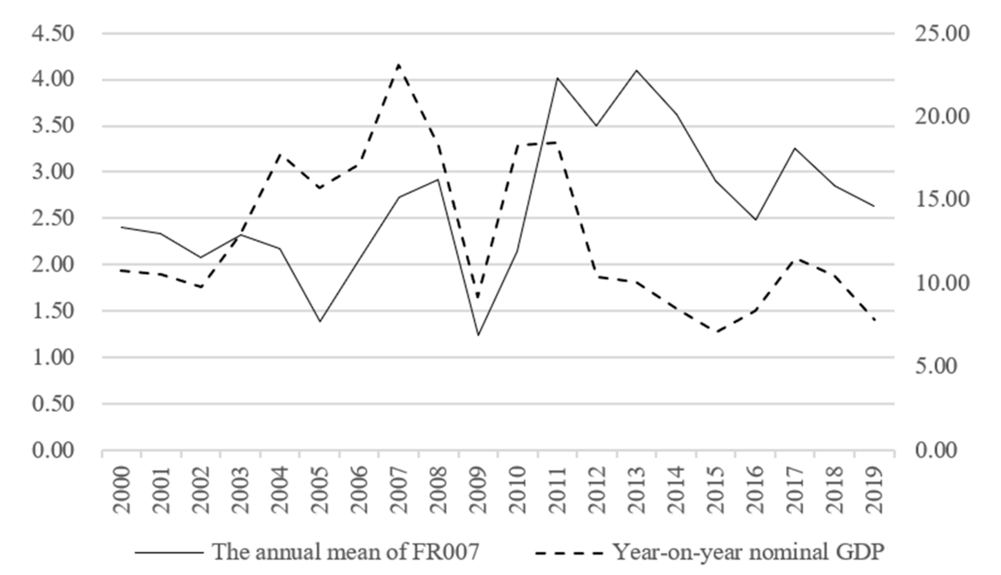
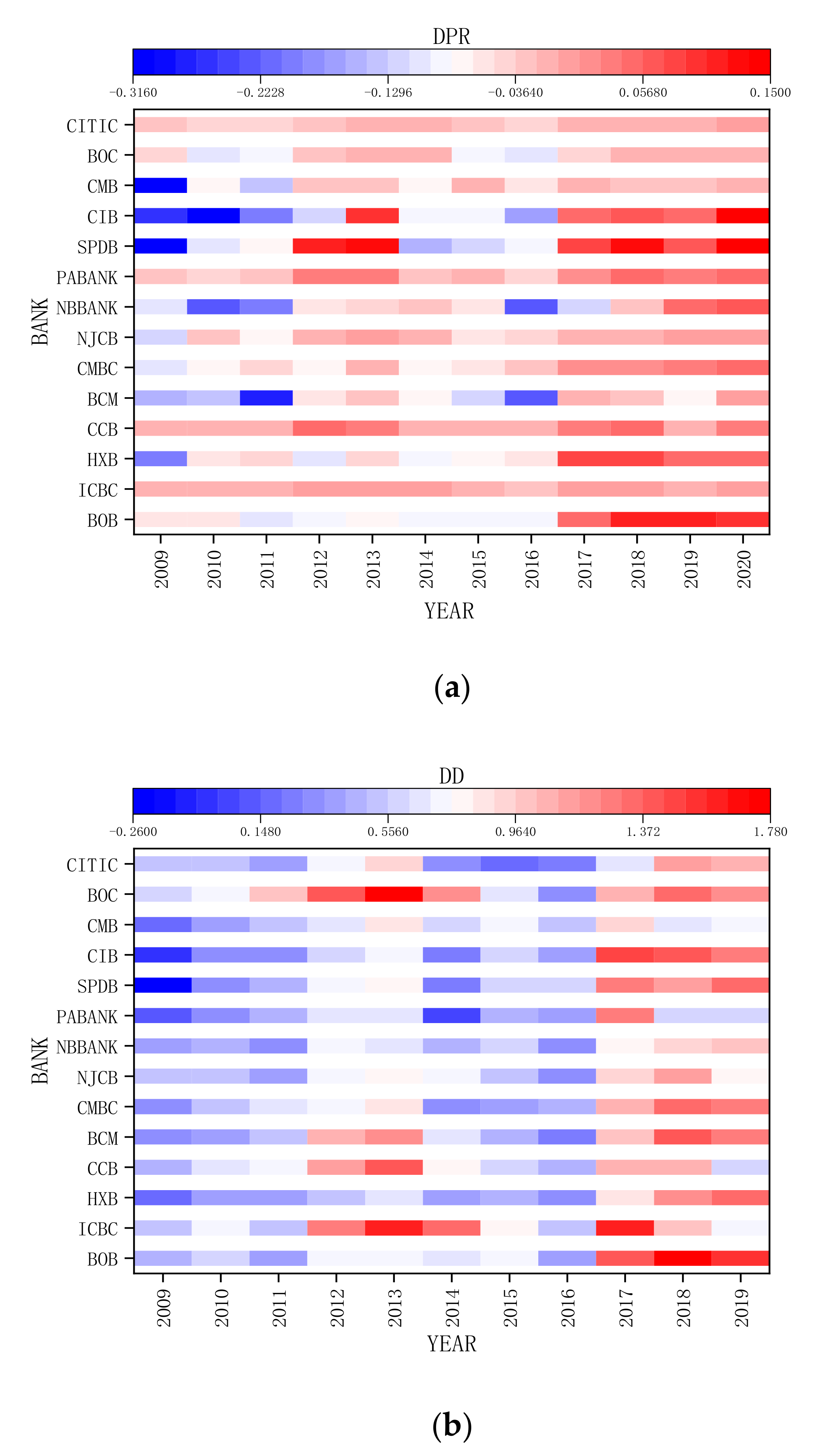
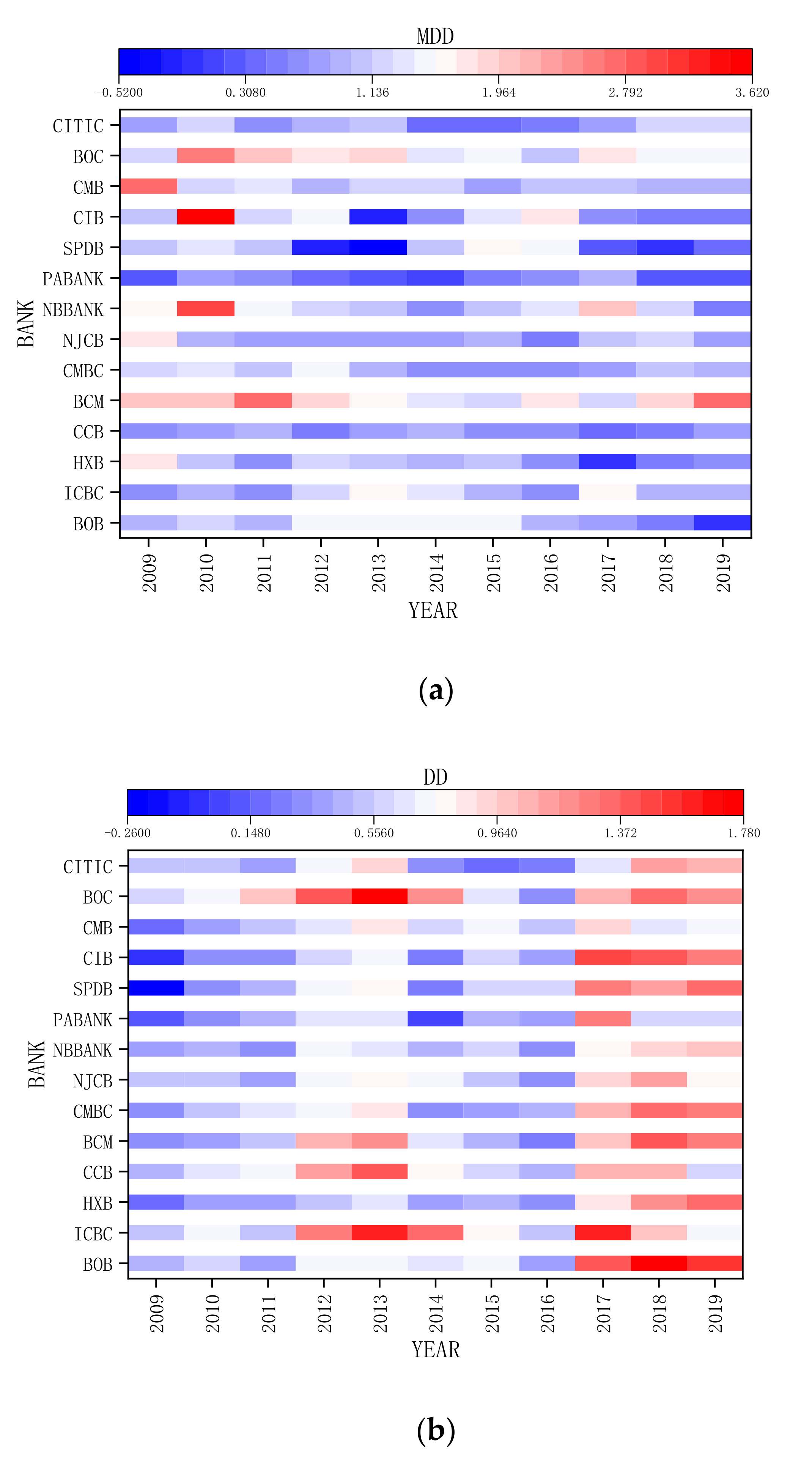
Table 1.
Setting method of forward-looking indicators.
| Indicator (Quarterly) | Abbreviation | Setting Method |
|---|---|---|
| Output gap | OG | The difference between real GDP year-on-year growth rate and potential GDP year-on-year growth rate |
| Inflation | I | Cumulative year-on-year GDP deflator |
| Unemployment rate | UR | Urban unemployment year-on-year growth rate |
| Foreign debt | FD | The ratio of quarterly increase in foreign debt balance to nominal GDP |
| Foreign exchange reserves | FER | The ratio of quarterly increase in foreign exchange reserves to nominal GDP |
| Foreign trade balance | FTB | The ratio of quarterly increase in current account balance to nominal GDP |
| Credit | C | Domestic non-financial sector credit year-on-year growth rate |
| Stock market | SM | The ratio of quarterly increase in total market value of A-shares to nominal GDP |
| Real estate market | REM | Cumulative new construction site area year-on-year growth rate |
Table 2.
Descriptive statistics.
| Indicators | Mean (%) | Maximum (%) | Minimum (%) | Median (%) | Standard Deviation (%) |
|---|---|---|---|---|---|
| OG | −0.0646 | 2.6092 | −4.4480 | −0.1800 | 1.2016 |
| I | 3.5862 | 9.2100 | −0.9800 | 3.1800 | 3.0763 |
| UR | 1.3456 | 10.9100 | −2.0100 | 0.5500 | 2.8118 |
| C | 16.1958 | 33.1500 | 10.1900 | 15.1400 | 5.2204 |
| FD | 0.0160 | 0.2900 | −0.0500 | 0.0100 | 0.0471 |
| FER | −0.0307 | 0.0600 | −0.1700 | −0.0200 | 0.0498 |
| FTB | 0.0309 | 0.1200 | −0.0100 | 0.0200 | 0.0280 |
| SM | 0.0269 | 1.0600 | −1.3100 | 0.0100 | 0.4100 |
| REM | 8.0788 | 34.1000 | −17.2744 | 7.4000 | 11.0717 |
| MES5%(BOB) | 2.8567 | 7.6825 | 0.2424 | 2.6778 | 1.6909 |
| MES5%(ICBC) | 2.3188 | 6.3178 | 0.4141 | 1.8245 | 1.6017 |
| MES5%(HXB) | 3.4414 | 9.0823 | 0.6441 | 3.0618 | 2.0274 |
| MES5%(CCB) | 2.5160 | 7.5438 | −1.1957 | 2.3547 | 1.8034 |
| MES5%(BCM) | 3.1825 | 8.8084 | 0.3155 | 2.8477 | 2.0020 |
| MES5%(CMBC) | 3.0042 | 7.5143 | 0.8844 | 2.4681 | 1.7294 |
| MES5%(NJCB) | 3.3603 | 9.8108 | 0.6306 | 2.8801 | 2.0746 |
| MES5%(NBBANK) | 3.5824 | 8.3472 | 1.1519 | 3.3139 | 1.8716 |
| MES5%(SPABANK) | 3.6243 | 7.8368 | 0.0000 | 3.1213 | 2.0302 |
| MES5%(SPDB) | 3.4216 | 8.2442 | 0.8305 | 2.7384 | 1.8345 |
| MES5%(CIB) | 3.4579 | 7.8659 | 0.7896 | 3.0855 | 1.9586 |
| MES5%(CMB) | 3.2992 | 9.4372 | 0.8803 | 2.8517 | 1.7329 |
| MES5%(BOC) | 2.1903 | 6.5244 | 0.1761 | 1.7219 | 1.4162 |
| MES5%(CITIC) | 3.4881 | 7.4035 | 0.8184 | 3.2361 | 1.8095 |
| DD(BOB) | 0.9203 | 1.7598 | 0.3859 | 0.7131 | 0.5080 |
| DD(ICBC) | 1.0059 | 1.6012 | 0.5011 | 0.8989 | 0.4069 |
| DD(HXB) | 0.6915 | 1.5740 | 0.1645 | 0.5097 | 0.4353 |
| DD(CCB) | 0.8437 | 1.3817 | 0.4464 | 0.7773 | 0.2990 |
| DD(BCM) | 0.8511 | 1.5797 | 0.2693 | 0.8324 | 0.4449 |
| DD(CMBC) | 0.7901 | 1.5887 | 0.2977 | 0.7179 | 0.4198 |
| DD(NJCB) | 0.7086 | 1.1121 | 0.3419 | 0.7307 | 0.2345 |
| DD(NBBANK) | 0.6362 | 1.0126 | 0.3022 | 0.6199 | 0.2449 |
| DD(SPABANK) | 0.5333 | 1.2552 | 0.0627 | 0.5279 | 0.3037 |
| DD(SPDB) | 0.7035 | 1.3419 | −0.2586 | 0.6655 | 0.4588 |
| DD(CIB) | 0.6777 | 1.4472 | 0.0034 | 0.5734 | 0.4535 |
| DD(CMB) | 0.6393 | 1.0232 | 0.1790 | 0.6745 | 0.2182 |
| DD(BOC) | 1.0909 | 1.7820 | 0.3374 | 1.1328 | 0.4348 |
| DD(CITIC) | 0.6415 | 1.1214 | 0.2089 | 0.6202 | 0.2989 |
Table 3.
Regression results on the probability of Event 1.
| Banks | c | OG | I | UR | C | FD | FER | FTB | SM | REM |
|---|---|---|---|---|---|---|---|---|---|---|
| BOB | −1.009 | −0.989 ** (0.017) | −0.446 ** (0.018) | — | — | — | — | — | 1.545 ** (0.025) | 0.053 * (0.063) |
| ICBC | −0.916 | −0.364 *(0.080) | — | — | — | — | — | — | — | 0.043 ** (0.039) |
| HXB | 0.055 | — | — | −0.281 ** (0.010) | — | — | — | — | 0.978 ** (0.042) | — |
| CCB | 2.832 | — | −0.370 *** (0.003) | — | −0.169 *** (0.008) | — | −19.971 *** (0.008) | — | — | — |
| BCM | 6.423 | −1.652 *** (0.005) | — | −0.326 * (0.063) | −0.450 *** (0.002) | — | — | −21.770 ** (0.038) | — | 0.049 * (0.081) |
| CMBC | 1.631 | −0.862 ** (0.027) | — | −0.445 ** (0.017) | −0.106 * (0.073) | — | — | — | 1.670 ** (0.013) | — |
| NJCB | 0.768 | — | −0.206 ** (0.010) | −0.302 ** (0.010) | — | — | — | — | — | — |
| NBBANK | 3.937 | −0.794 ** (0.013) | — | — | −0.271 *** (0.004) | — | — | −28.101 *** (0.009) | — | 0.063 ** (0.020) |
| SPABANK | 2.187 | −0.853 *** (0.002) | — | — | −0.216 *** (0.000) | — | — | — | 1.764 ** (0.010) | 0.095 *** (0.002) |
| SPDB | −0.308 | — | — | −0.210 * (0.055) | — | — | — | — | — | — |
| CIB | 3.410 | −0.811 * (0.068) | — | −0.286 * (0.069) | −0.267 ** (0.020) | — | — | — | — | 0.046 * (0.053) |
| CMB | 0.566 | — | −0.272 *** (0.003) | −0.336 * (0.052) | — | — | — | — | — | — |
| BOC | 1.871 | — | −0.301 *** (0.007) | — | −0.133 ** (0.038) | — | −17.849 ** (0.011) | — | — | — |
| CITIC | 2.673 | — | −0.147 * (0.057) | — | −0.183 *** (0.006) | — | — | — | — | 0.051 ** (0.018) |
***, **, * indicate significance at the 0.01, 0.05, and 0.10 level, respectively.
Table 4.
Regression results on the probability of Event 2.
| Banks | c | OG | I | UR | C | FD | FER | FTB | SM | REM | ||
|---|---|---|---|---|---|---|---|---|---|---|---|---|
| BOB | −1.041 | 0.525 * (0.053) | — | — | — | — | −12.146 * (0.082) | — | — | −0.070 * (0.090) | ||
| ICBC | −0.512 | — | — | — | −0.10973 ** (0.048) | — | −18.604 ** (0.039) | — | — | — | ||
| HXB | −1.363 | — | — | — | — | — | — | 17.058 ** (0.018) | — | — | ||
| CCB | −1.740 | — | −0.137 * (0.098) | — | — | — | — | 18.986 ** (0.017) | −1.586 ** (0.050) | — | ||
| BCM | 17.039 | — | — | 40.511 *** (0.000) | −18.374 *** (0.000) | −139.812 *** (0.000) | −125.262 *** (0.000) | 4640.601 *** (0.000) | — | −6.800 *** (0.000) | ||
| CMBC | 15.192 | — | — | 2.146 ** (0.023) | −1.518 ** (0.014) | — | −116.758 *** (0.009) | — | — | −0.252 ** (0.015) | ||
| NJCB | −0.455 | 1.212 *** (0.002) | −0.379 ** (0.012) | — | — | −53.973 *** (0.007) | −18.660 * (0.074) | 27.735 ** (0.014) | −2.464 ** (0.023) | — | ||
| NBBANK | −1.235 | — | −0.289 *** (0.005) | — | — | — | — | 38.942 *** (0.000) | −2.147 *** (0.001) | — | ||
| SPABANK | −1.335 | — | — | — | — | — | — | 20.222 *** (0.000) | −1.474 ** (0.024) | — | ||
| SPDB | −1.756 | — | — | 0.173 ** (0.011) | — | — | — | 18.484 ** (0.015) | — | — | ||
| CIB | −1.705 | — | — | 0.173 ** (0.011) | — | — | — | 18.484 ** (0.015) | — | — | ||
| CMB | −1.591 | — | — | 48.593 *** (0.000) | −20.831 *** (0.000) | −107.995 *** (0.000) | — | 5558.682 *** (0.000) | — | −6.903 *** (0.000) | ||
| BOC | 0.255 | — | — | — | −0.1296 ** (0.014) | −12.846 ** (0.035) | — | — | — | — | ||
| CITIC | 1.038 | 0.451 ** (0.019) | −0.231 * (0.072) | — | −0.125 * (0.072) | — | −15.914 * (0.099) | 17.250 ** (0.041) | — | — | ||
***, **, * indicate significance at the 0.01, 0.05, and 0.10 level, respectively.
Table 5.
The correlation coefficients in the binary Gaussian Copula model.
| BANK | EVENT 1 | EVENT 2 |
|---|---|---|
| BOB | 0.373 | −0.367 |
| ICBC | 0.023 | −0.064 |
| HXB | −0.522 | 0.496 |
| CCB | −0.120 | 0.266 |
| BCM | −0.489 | −0.218 |
| CMBC | −0.337 | 0.113 |
| NJCB | −0.354 | −0.044 |
| NBBANK | −0.400 | 0.316 |
| SPABANK | −0.150 | 0.224 |
| SPDB | −0.549 | 0.609 |
| CIB | −0.502 | 0.474 |
| CMB | −0.527 | −0.103 |
| BOC | −0.140 | −0.354 |
| CITIC | −0.185 | −0.083 |
Publisher’s Note: MDPI stays neutral with regard to jurisdictional claims in published maps and institutional affiliations. |
© 2020 by the authors. Licensee MDPI, Basel, Switzerland. This article is an open access article distributed under the terms and conditions of the Creative Commons Attribution (CC BY) license (http://creativecommons.org/licenses/by/4.0/).
Share and Cite
MDPI and ACS Style
Hui, X.; Zhang, A. Construction and Empirical Research on the Dynamic Provisioning Model of China’s Banking Sector under the Macro-Prudential Framework. Sustainability 2020, 12, 8527. https://doi.org/10.3390/su12208527
AMA Style
Hui X, Zhang A. Construction and Empirical Research on the Dynamic Provisioning Model of China’s Banking Sector under the Macro-Prudential Framework. Sustainability. 2020; 12(20):8527. https://doi.org/10.3390/su12208527
Chicago/Turabian StyleHui, Xiaofeng, and Aoran Zhang. 2020. "Construction and Empirical Research on the Dynamic Provisioning Model of China’s Banking Sector under the Macro-Prudential Framework" Sustainability 12, no. 20: 8527. https://doi.org/10.3390/su12208527
Note that from the first issue of 2016, this journal uses article numbers instead of page numbers. See further details here.