The Stochastic Annuity Method for Supporting Maintenance Costs Planning and Durability in the Construction Sector: A Simulation on a Building Component


Abstract
:1. Introduction
2. Literature and Regulatory Background
2.1. The Regulatory Framework
- ISO 15686-5:2008, Buildings and Constructed Assets—Service Life planning—Part 5: Life Cycle Costing (revised July 2017—ISO 15686-5:2017) [3];
- ISO 15686-1:2000, Building and constructed assets—Service Life planning—Part 1: General principles (revised by 15686-1:2011) [6];
- ISO 15686-2:2001, Building and constructed assets—Service Life planning—Part 2: Service Life prediction procedures (revised by 15686-2:2012) [7];
- ISO 15686-7:2006, Building and constructed assets—Service Life planning—Part 7: Performance Evaluation for Feed-back of Service Life data from practice (revised by 15686-7:2017) [8];
- ISO 15686-8:2008, Building and constructed assets—Service Life planning—Part 8: Reference Service Life and Service Life estimation [9].
- Furthermore:
- UNI 11156-3: 2006, Valutazione della durabilità dei componenti edilizi. Metodo per la valutazione della durata (vita utile) [10];
- Standard EN 15459-1:2017—Energy performance of buildings—Economic evaluation procedure for energy systems in buildings (repealed by UNI EN 15459-1:2018) [4];
- Guidelines accompanying Commission Delegated Regulation (EU) No 244/2012 [11];
- Directive 2010/31/EU of the European Parliament and of the Council of 19 May 2010 on the energy performance of buildings—recast (revised by Directive 2018/844/EU—EPBD recast) [12].
2.2. The International Literature
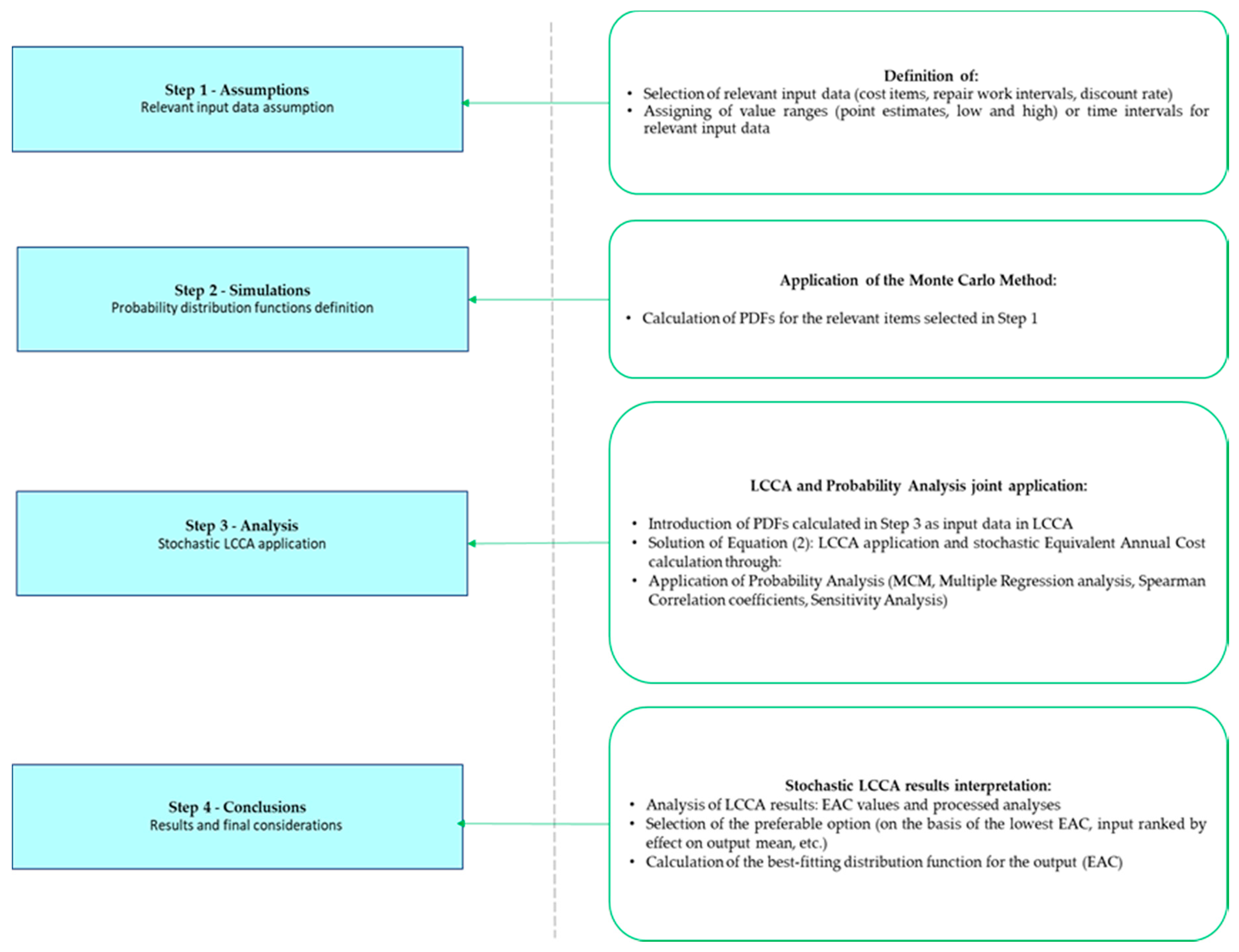
3. Methodology
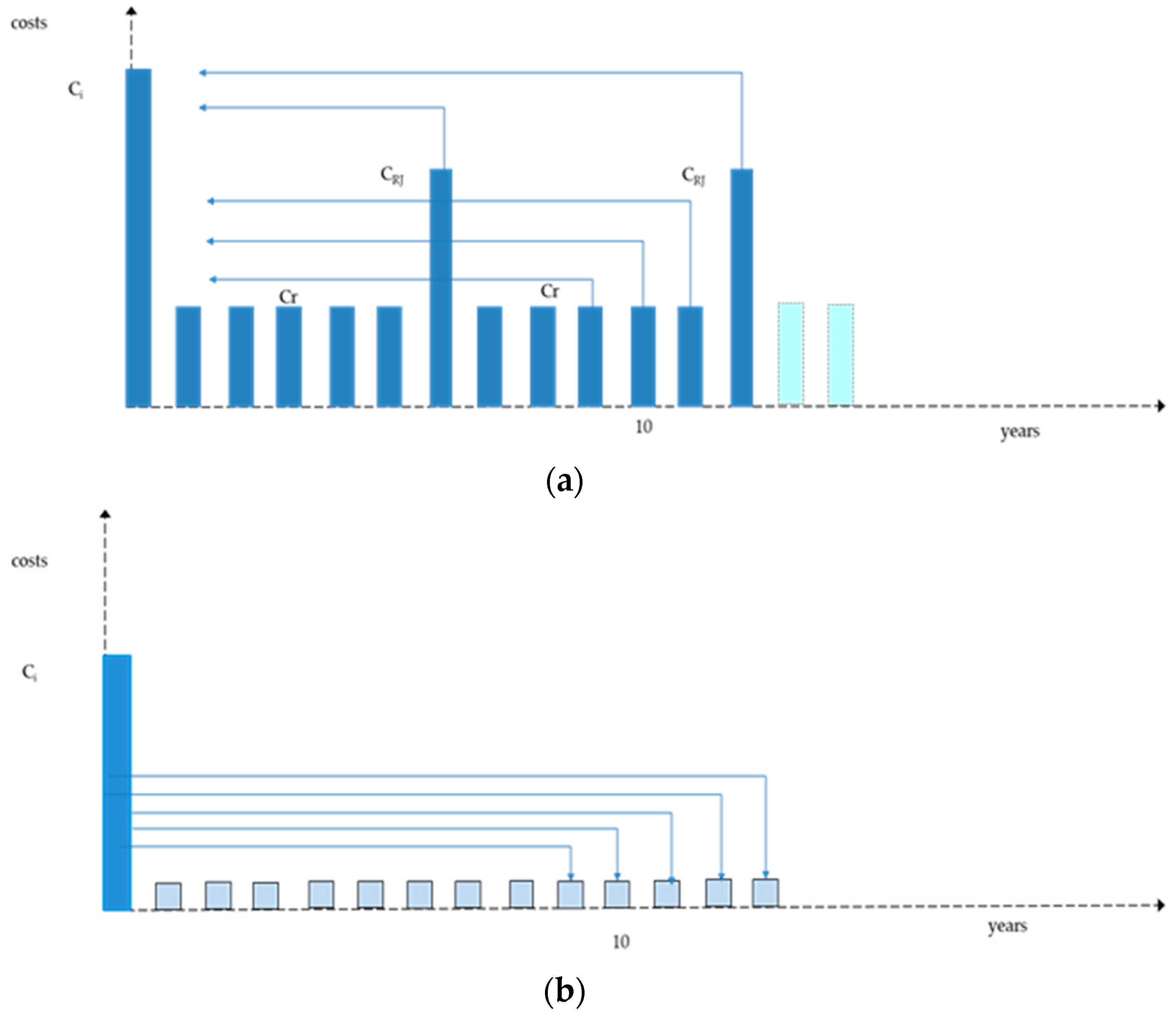
3.1. The Annuity Method Approach
- –
- running costs, generally constant over time;
- –
- replacement costs (or extraordinary maintenance costs), periodically distributed, related to components or systems with a service life lower or higher than the building life cycle.
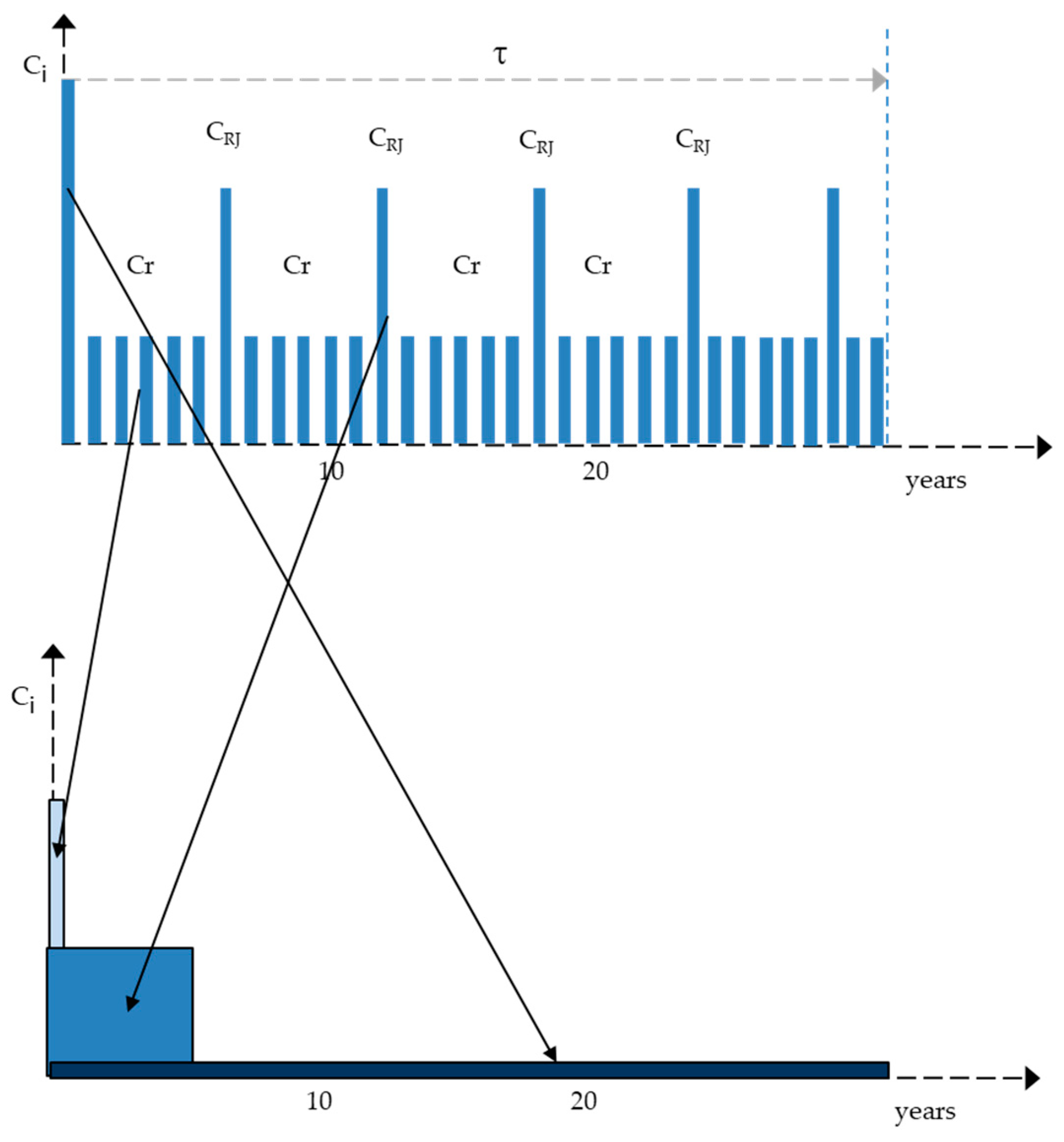
3.2. The Stochastic Annuity Method Approach
3.3. The Life Cycle Costing Approach
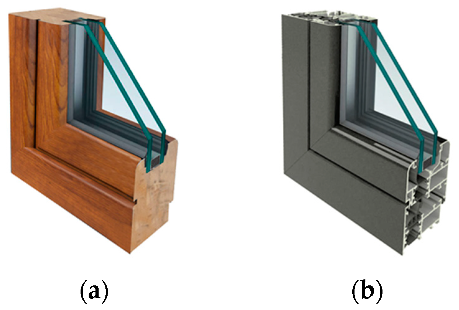
4. Case Study
5. Simulation and Results
5.1. Input Data Assumptions and Probability Distribution Functions Calculation
- –
- Firstly, a higher probability for repairing/replacement time intervals reduction is considered, and a lower probability for repairing/replacement time intervals lengthening;
- –
- Secondly, a noticeable reduction on the time intervals for Timber Frame, considering a lower durability degree as respect to Aluminum Frame.
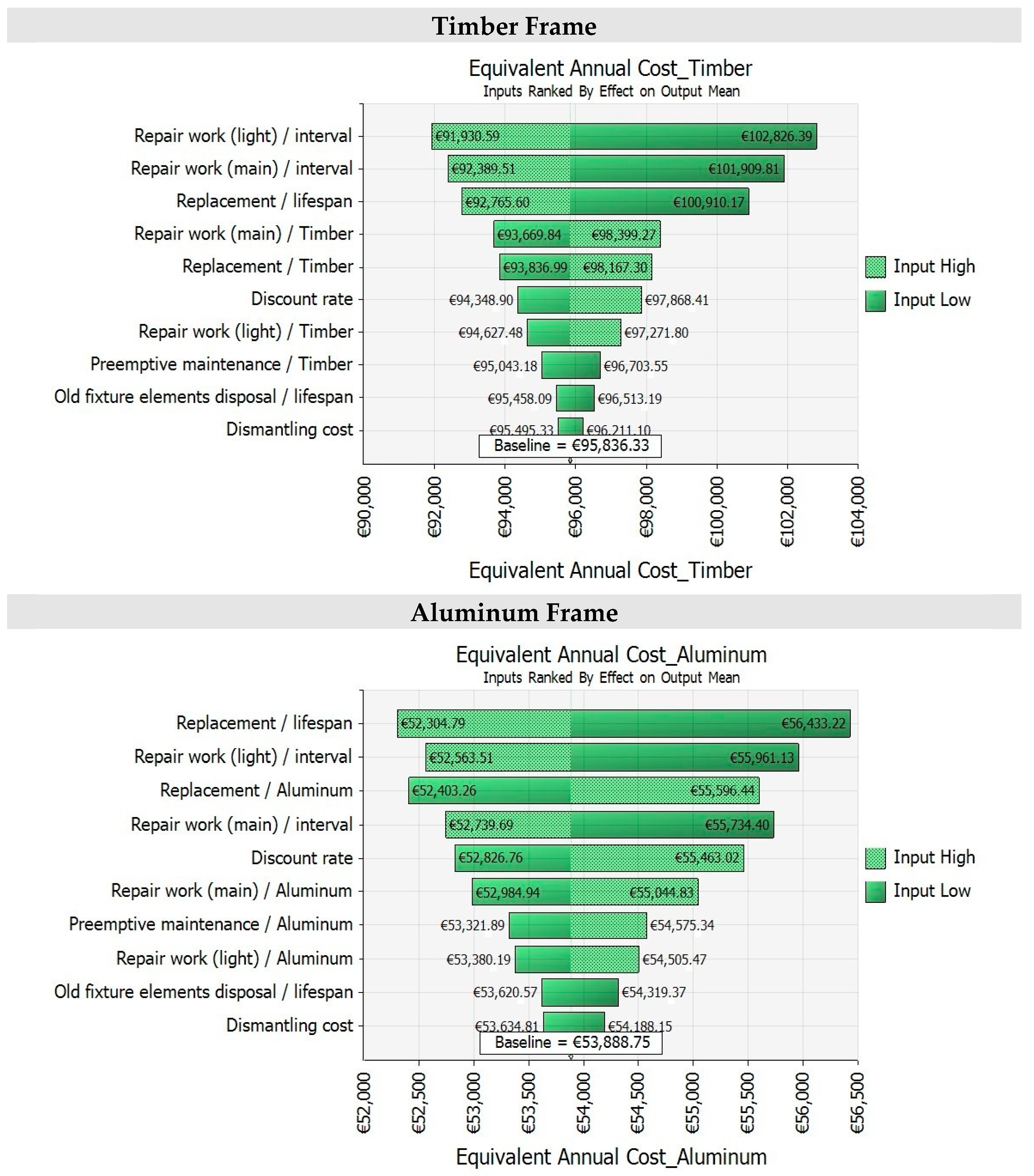
5.2. Stochastic Equivalent Annual Cost Calculation in Life Cycle Cost Analysis
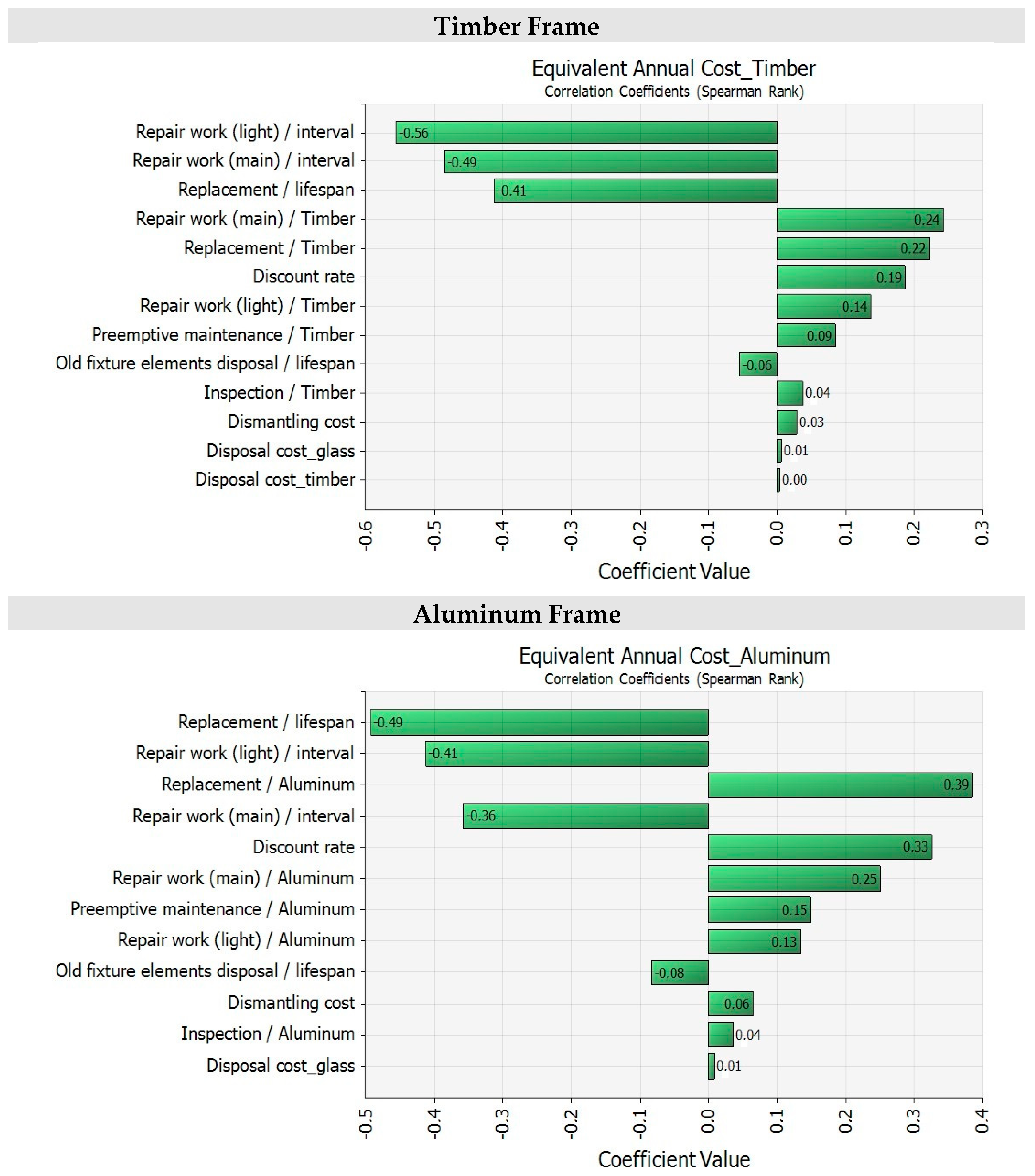
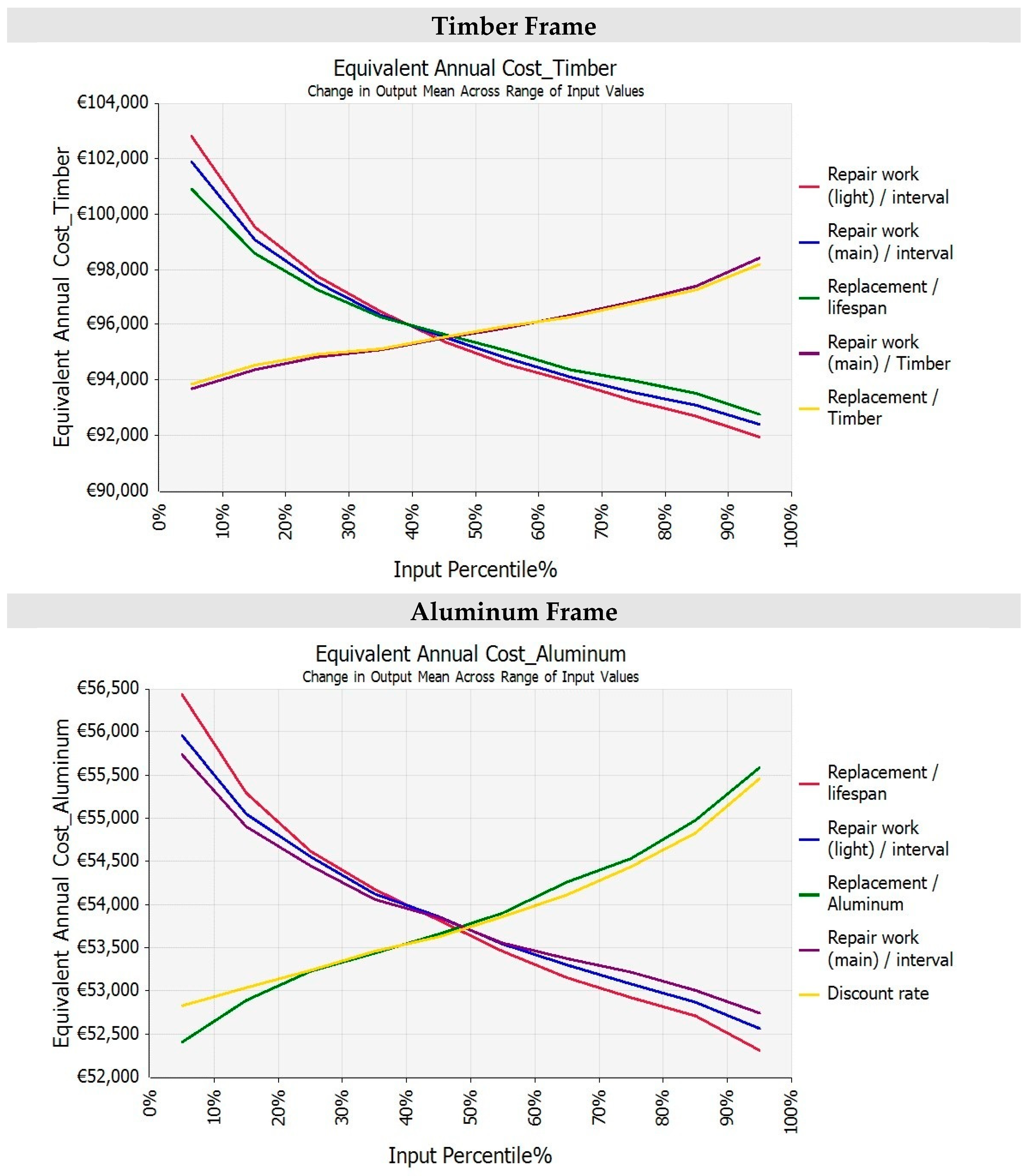
5.3. Stochastic LCCA Results and Final Considerations
6. Conclusions
Author Contributions
Funding
Acknowledgments
Conflicts of Interest
References
- Farahani, A.; Wallbaum, H.; Dalenback, J.O. Optimized Maintenance and Renovation Scheduling in Multifamily Buildings—A Systematic Approach Based on Condition State and Life Cycle Cost of Building Components. Constr. Manag. Econ. 2018, 37, 3. [Google Scholar] [CrossRef] [Green Version]
- Sarja, A. Predictive and Optimised Life Cycle Management. Buildings and Infrastructure; Taylor & Francis: Oxon, UK, 2006. [Google Scholar]
- International Organization for Standardization. ISO 15686:2008—Buildings and Constructed Assets—Service-Life Planning—Part 5: Life Cycle Costing. ISO/TC 59/CS 14; International Organization for Standardization: Geneva, Switzerland, 2008. [Google Scholar]
- European Committee for Standardization (CEN). Standard EN ISO 15459-1:2017. Energy Performance of Buildings—Economic Evaluation Procedure for Energy Systems in Buildings; European Committee for Standardization: Brussels, Belgium, 2017. [Google Scholar]
- Fregonara, E.; Giordano, R.; Ferrando, D.G.; Pattono, S. Economic-Environmental Indicators to Support Investment Decisions: A Focus on the Buildings’ End-of-Life Stage. Buildings 2017, 7, 65. [Google Scholar] [CrossRef] [Green Version]
- International Organization for Standardization. ISO 15686-1:2000, Building and Constructed Assets—Service Life Planning—Part 1: General Principles; International Organization for Standardization: Geneva, Switzerland, 2000. [Google Scholar]
- International Organization for Standardization. ISO 15686-2:2001, Building and Constructed Assets—Service Life Planning—Part 2: Service Life Prediction Procedures; International Organization for Standardization: Geneva, Switzerland, 2001. [Google Scholar]
- International Organization for Standardization. ISO 15686-7:2006, Building and Constructed Assets—Service Life Planning—Part 7: Performance Evaluation for Feed-Back of Service Life Data from Practice; International Organization for Standardization: Geneva, Switzerland, 2006. [Google Scholar]
- International Organization for Standardization. ISO 15686-8:2008, Building and Constructed Assets—Service Life Planning—Part 8: Reference Service Life and Service Life Estimation; International Organization for Standardization: Geneva, Switzerland, 2008. [Google Scholar]
- Italian Organization for Standardization. UNI 11156-3: 2006, Valutazione Della Durabilità dei Componenti Edilizi. Metodo per la Valutazione Della Durata (Vita Utile); Italian Organization for Standardization (UNI): Milan, Italy, 2006. [Google Scholar]
- European Parliament. Guidelines Accompanying Commission Delegated Regulation (EU) No 244/2012 of 16 January 2012 Supplementing Directive 2010/31/EU; European Parliament: Brussels, Belgium, 2012. [Google Scholar]
- European Parliament. Directive 2010/31/EU of the European Parliament and of Council of 19 May 2010 on the Energy Performance of Buildings (Recast); Official Journal of the European Union: Brussels, Belgium, 2010; Available online: https://eur-lex.europa.eu/LexUriServ/LexUriServ.do?uri=OJ:L:2010:153:0013:0035:EN:PDF (accessed on 3 April 2020).
- Flanagan, R.; Kendell, A.; Norman, G.; Robinson, G.D. Life cycle costing and risk management. Constr. Manag. Econ. 1987, 5, 53–71. [Google Scholar] [CrossRef]
- Boussabaine, A.; Kirkham, R. Whole Life-Cycle Costing: Risk and Risk Responses; Blackwell Publising: Oxford, UK, 2004; pp. 56–83, 142–162. [Google Scholar]
- Fregonara, E.; Ferrando, D.G.; Pattono, S. Economic–Environmental Sustainability in Building Projects: Introducing Risk and Uncertainty in LCCE and LCCA. Sustainability 2018, 10, 1901. [Google Scholar] [CrossRef] [Green Version]
- Curto, R.A.; Fregonara, E. Decision Tools for Investiments in the Real Estate Sector with Risk and Uncertainty Elements, Jahrbuch für Regionalwissenschaft 1999; Springer: Heidelberg, Germany, 1999. [Google Scholar]
- Wang, N.; Chang, Y.C.; El-Sheikh, A. Monte Carlo simulation approach to life cycle cost management. Struct. Infrastruct. Eng. 2012, 8, 739–746. [Google Scholar] [CrossRef]
- Jafari, A.; Valentin, V.; Russell, M. Probabilistic Life Cycle Cost Model for Sustainable Housing Retrofit Decision- Making. In Proceedings of the International Conference on Computing in Civil and Building Engineering, Orlando, FL, USA, 23–25 June 2014; pp. 1925–1933. [Google Scholar]
- Oduyemi, O.; Okoroh, M.; Fajana, O.S. Risk assessment methods for life cycle costing in buildings. Sustain. Build. 2016, 1, 9–18. [Google Scholar] [CrossRef] [Green Version]
- Bourke, K.; Davies, H. Factors Affecting Service Life Predictions of Buildings: A Discussion Paper. Laboratory Report—Building Research Establishment; Garston: Watford, UK, 1997. [Google Scholar]
- Shohet, I.M.; Puterman, M.; Gilboa, E. Deterioration patterns of building cladding components for maintenance management. Constr. Manag. Econ. 2002, 20, 305–314. [Google Scholar] [CrossRef]
- Hovde, P.J.; Moser, K. Performance Based Methods for Service Life Prediction; International Council for Research and Innovation in Building and Construction: Rotterdam, The Netherlands, 2004. [Google Scholar]
- Kumar, D.; Setunge, S.; Patnaikuni, I. Prediction of life-cycle expenditure for different categories of council buildings. J. Perform. Constr. Facil. 2010, 24, 556–561. [Google Scholar] [CrossRef]
- Flint, M.; Baker, J.; Billington, S. A Probabilistic Framework for Performance-based Durability Engineering. In Durability of Building Materials and Components. Building Pathology and Rehabilitation; De Freitas, V., Delgado, J., Eds.; Springer: Berlin, Germany, 2013; Volume 3. [Google Scholar]
- Fregonara, E.; Ferrando, D.G. How to Model Uncertain Service Life and Durability of Components in Life Cycle Cost Analysis Applications? The Stochastic Approach to the Factor Method. Sustainability 2018, 10, 10. [Google Scholar] [CrossRef] [Green Version]
- König, H.; Kohler, N.; Kreissig, J.; Lützkendorf, T. A Life Cycle Approach to Buildings. Principles, Calculations, Design Tools; Detail Green Books: Regensburg, Germany, 2010. [Google Scholar]
- Hoff, J.L. Equivalent Uniform Annual Cost: A New Approach to Roof Life Cycle Analysis. Available online: https://epdmroofs.org/wp-content/uploads/2018/04/2007_01_anewapproachtorooflifecycleanalysis_interface_jimhoff.pdf (accessed on 3 April 2020).
- Schade, J. Life cycle cost calculation models for buildings. In Proceedings of the 4th Nordic Conference on Construction Economics and Organisation: Development Processes in Construction Mangement, Luleå Tekniska Universitet, Luleå, Sweden, 14–15 June 2007; pp. 321–329. [Google Scholar]
- Marszal, A.J.; Heiselberg, P. Life cycle cost analysis of a multi-storey residential Net Zero Energy Building in Denmark. Energy 2011, 36, 5600–5609. [Google Scholar] [CrossRef]
- Plebankiewicz, E.; Zima, K.; Wieczorek, D. Life Cycle Equivalent Annual Cost (LCEAC) as a Comparative Indicator in the Life Cycle Cost Analysis of Buildings with Different Lifetimes. MATEC Web Conf. 2018, 196. [Google Scholar] [CrossRef]
- Flanagan, R.; Norman, G. Life Cycle Costing for Construction; Royal Institution of Chartered Surveyors: London, UK, 1983. [Google Scholar]
- Department of Energy (DOE). Life Cycle Cost Handbook Guidance for Life Cycle Cost Estimate and Life Cycle Cost Analysis; Department of Energy (DOE): Washington, DC, USA, 2014. [Google Scholar]
- Fregonara, E.; Lo Verso, V.R.M.; Lisa, M.; Callegari, G. Retrofit Scenarios and Economic Sustainability. A Case-study in the Italian Context. Energy Procedia 2017, 111, 245–255. [Google Scholar]
- Maio, C.; Schexnayder, C.; Knutson, K.; Weber, S. Probability distribution function for construction simulation. J. Constr. Eng. Manag. 2000, 126, 285–292. [Google Scholar] [CrossRef]
- Sarja, A. Life Cycle Management of Concrete Infrastructures for Improved Sustainability. Available online: https://www.irbnet.de/daten/iconda/CIB5503.pdf (accessed on 3 April 2020).


| Timber Frame | Aluminum Frame | ||||||
|---|---|---|---|---|---|---|---|
| Input Data | Unit | Low Range | Point Estimate | High Range | Low Range | Point Estimate | High Range |
| Inspection | € per year | 6220 | 6547 | 7202 | 2253 | 2372 | 2609 |
| Preemptive maintenance | € per year | 15,550 | 16,369 | 18,005 | 11,267 | 11,860 | 13,046 |
| Repair work (light) | € | 62,201 | 65,474 | 72,022 | 45,067 | 47,439 | 52,183 |
| Repair work (light) interval | years | 1.8 | 3 | 3.3 | 3.5 | 5 | 5.5 |
| Repair work (main) | € | 117,854 | 130,949 | 157,138 | 74,717 | 83,019 | 99,622 |
| Repair work (main) interval | years | 4.2 | 7 | 7.7 | 7 | 10 | 11 |
| Replacement | € | 339,561 | 377,290 | 452,748 | 258,404 | 287,115 | 344,538 |
| Replacement interval (lifespan) | years | 15 | 25 | 30 | 17.5 | 25 | 27.5 |
| Dismantling cost | €/m2 | 29.7 | 33 | 39.6 | 29.7 | 33 | 39.6 |
| Disposal cost | €/ton | 49.5 | 55 | 66 | −640 | −800 | −880 |
| Dismantling/disposal interval | years | 15 | 25 | 30 | 17.5 | 25 | 27.5 |
| Discount rate | % | 1.25 | 1.39 | 2.50 | 1.25 | 1.39 | 2.50 |
| Input Data | Distribution | Graph | Min | Mean | Max | 5% | 95% |
|---|---|---|---|---|---|---|---|
| Disposal cost_glass | Triangular |  | 72.04 | 82.67 | 95.96 | 75.1 | 91.62 |
| Disposal cost_timber | Triangular |  | 49.52 | 56.83 | 65.96 | 51.63 | 62.99 |
| Disposal cost_aluminum | Triangular |  | 640.15 | 773.33 | 879.75 | 683.82 | 849.02 |
| Dismantling cost | Triangular |  | 29.7 | 34.1 | 39.57 | 30.98 | 37.79 |
| Discount rate | Triangular |  | 1.25% | 1.71% | 2.5% | 1.34% | 2.24% |
| Inspection cost (€): | |||||||
| Timber | Triangular |  | 6221 | 6657 | 7201 | 6347 | 7023 |
| Aluminum | Triangular |  | 2254 | 2411 | 2608 | 2299 | 2544 |
| Preemptive maintenance cost (€): | |||||||
| Timber | Triangular |  | 15,554 | 16,641 | 17,999 | 15,867 | 17,557 |
| Aluminum | Triangular |  | 11,268 | 12,057 | 13,042 | 11,496 | 12,721 |
| Repair work (light) cost (€): | |||||||
| Timber | Triangular |  | 62,214 | 66,565 | 71,998 | 63,468 | 70,228 |
| Aluminum | Triangular |  | 45,078 | 48,230 | 52,181 | 45,986 | 50,884 |
| Repair work (light) interval (years): | |||||||
| Timber | Triangular |  | 1.8 | 2.7 | 3.3 | 2.1 | 3.15 |
| Aluminum | Triangular |  | 3.5 | 4.67 | 5.5 | 3.89 | 5.28 |
| Repair work (main) cost (€): | |||||||
| Timber | Triangular |  | 117,889 | 135,313 | 157,043 | 122,925 | 149,965 |
| Aluminum | Triangular |  | 74,759 | 85,786 | 99,608 | 77,932 | 95,075 |
| Repair work (main) interval (years): | |||||||
| Timber | Triangular |  | 4.20 | 6.30 | 7.70 | 4.90 | 7.35 |
| Aluminum | Triangular |  | 7 | 9.33 | 11 | 7.77 | 10.55 |
| Replacement cost (€): | |||||||
| Timber | Triangular |  | 339,753 | 389,866 | 452,604 | 354,172 | 432,083 |
| Aluminum | Triangular |  | 258,506 | 296,685 | 344,449 | 269,523 | 328,812 |
| Replacement interval (years): | |||||||
| Timber | Triangular |  | 15.02 | 23.33 | 29.98 | 17.74 | 28.06 |
| Aluminum | Triangular |  | 17.53 | 23.33 | 27.49 | 19.44 | 26.38 |
| Old fixture elements disposal interval (years) | |||||||
| Timber | Triangular |  | 15.01 | 23.33 | 29.97 | 17.74 | 28.06 |
| Aluminum | Triangular |  | 17.52 | 23.33 | 27.49 | 19.44 | 26.38 |
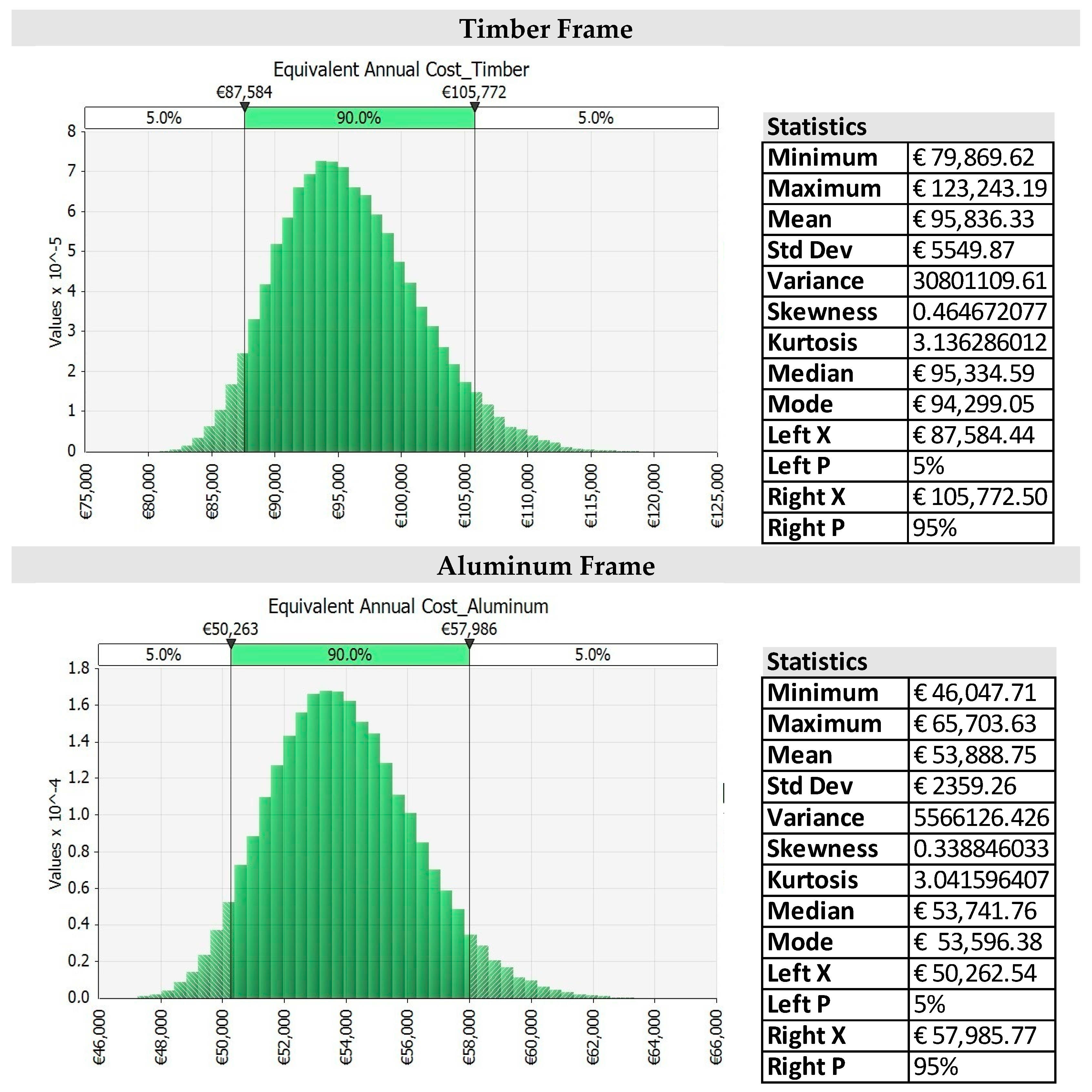
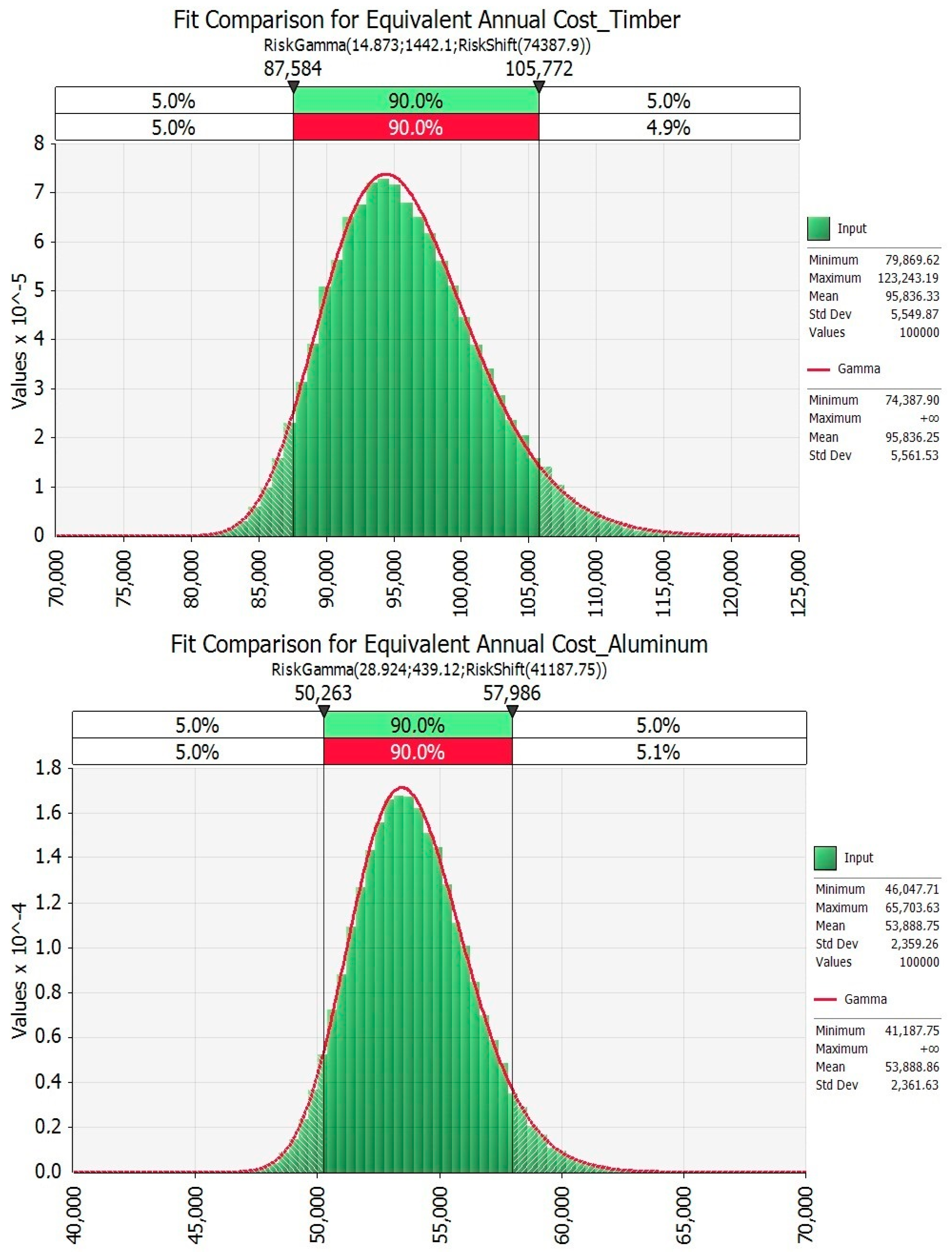
| Output | Graph | Min | Mean | Max | 5% | 95% |
|---|---|---|---|---|---|---|
| Equivalent Annual Cost_Timber |  | € 79,870 | € 95,836 | € 123,243 | € 87,584 | € 105,772 |
| Equivalent Annual Cost_Aluminum |  | € 46,048 | € 53,889 | € 65,704 | € 50,263 | € 57,986 |
© 2020 by the authors. Licensee MDPI, Basel, Switzerland. This article is an open access article distributed under the terms and conditions of the Creative Commons Attribution (CC BY) license (http://creativecommons.org/licenses/by/4.0/).
Share and Cite
Fregonara, E.; Ferrando, D.G. The Stochastic Annuity Method for Supporting Maintenance Costs Planning and Durability in the Construction Sector: A Simulation on a Building Component. Sustainability 2020, 12, 2909. https://doi.org/10.3390/su12072909
Fregonara E, Ferrando DG. The Stochastic Annuity Method for Supporting Maintenance Costs Planning and Durability in the Construction Sector: A Simulation on a Building Component. Sustainability. 2020; 12(7):2909. https://doi.org/10.3390/su12072909
Chicago/Turabian StyleFregonara, Elena, and Diego Giuseppe Ferrando. 2020. "The Stochastic Annuity Method for Supporting Maintenance Costs Planning and Durability in the Construction Sector: A Simulation on a Building Component" Sustainability 12, no. 7: 2909. https://doi.org/10.3390/su12072909