Physical Fatigue Detection Using Entropy Analysis of Heart Rate Signals

Abstract

Physical fatigue is one of the most important and highly prevalent occupational hazards in different industries. This research adopts a new analytical framework to detect workers’ physical fatigue using heart rate measurements. First, desired features are extracted from the heart signals using different entropies and statistical measures. Then, a feature selection method is used to rank features according to their role in classification. Finally, using some of the frequently used classification algorithms, physical fatigue is detected. The experimental results show that the proposed method has excellent performance in recognizing the physical fatigue. The achieved accuracy, sensitivity, and specificity rates for fatigue detection are 90.36%, 82.26%, and 96.2%, respectively. The proposed method provides an efficient tool for accurate and real-time monitoring of physical fatigue and aids to enhance workers’ safety and prevent accidents. It can be useful to develop warning systems against high levels of physical fatigue and design better resting times to improve workers’ safety. This research ultimately aids to improve social sustainability through minimizing work accidents and injuries arising from fatigue.

1. Introduction

The safer and healthier a workplace is, the fewer probabilities of diseases, accidents, injuries, and low performance [1]. Each day, an average of 6000 people die as a result of work-related accidents or diseases, totaling more than 2.2 million work-related deaths a year [2]. Of these, about 350,000 deaths are from workplace accidents, and more than 1.7 million are from work-related diseases [2]. Studies and estimates by many countries and the International Labor Organization (ILO) have shown that the economic costs of work-related illness and injury would be equivalent to a range of 1.8%–6% of gross domestic product (GDP) [3].

Physical fatigue is the ephemeral inability of muscles to maintain ideal physical performance, and results from prolonged activity [4,5,6]. It is one of the most important and highly prevalent occupational hazards in different industries [5,7]. Fatigue can occur due to excessive physical workload and results in a temporary reduction in the capability of physical activities [8]. Fatigue is one of the major sources for reduction in productivity, poor quality of work, injuries, and accidents in workplaces [9,10]. According to the World Health Organization, in recent years, the effects of physical fatigue on human health have been accumulating. Although “tiredness” has been reported as a construction accident risk by several studies, less attention was paid to this risk [5]. Fatigue affects workers’ health and safety and needs to be measured and controlled to prevent severe injuries.

In recent years, several studies have been conducted to assess physical workload and fatigue in construction projects using various subjective and objective methods. In most of the previous studies, subjective methods, including interviews [5] and questionnaires [6,11], have been used. The subjective methods used in previous studies do not provide broad insights into the adverse effects of physical fatigue and have several disadvantages. For example, they may suffer from subjective bias, and some people may answer in such a way to support the researcher’s hypothesis [6,11,12]. Therefore, a significant shift in the methods and tools adopted in previous research is needed. Measurement of the physiological responses which are less susceptible to participant bias represents a viable alternative and objective method to measure the impacts of physical fatigue. The use of physiological measurements, in addition to questionnaires, is the fundamental step change that this research area requires to establish a defensible evidence base for producing safety guidelines regarding the impact of physical fatigue on human health.

The previous studies harnessed physiological signals to estimate fatigue level, since it results from physical overexertion and is associated with physiological symptoms [8]. In the previous studies, heart rate, oxygen consumption, muscle activity, skin temperature, electrodermal (EDA) activity, blood pressure, and inertial measurement units were used to assess physical fatigue [13,14,15,16,17,18,19]. Chang et al. [20] investigated the relationship between the heart rate and fatigue and suggested heart rate as an indicator to predict the extent of strains or hazards which construction workers encounter [20]. Aryal et al. [21] used heart rate, skin temperature, and an electroencephalogram (EEG) sensor to assess the level of fatigue. The classification accuracy based on features extracted from the average of skin temperature and heart rate data was 82% [21]. Maman et al. [22] used inertial measurement units (IMUs) and developed a data-driven approach to assess workers’ fatigue in simulated manufacturing tasks. Important features from the five sensor locations were selected, and they achieved high accuracy in estimating the Ratings of Perceived Exertions (RPE) scale [22]. Jebelli et al. [18] used EDA, skin temperature (ST), and a photoplethysmogram (PPG) to assess workers’ physical states under different workloads. The heart rate variability, percentage heart rate, and EDA level showed a clear difference in light and medium tasks [18]. Zhang et al. [23] assessed the feasibility of using jerk, the time derivative of acceleration, as an indicator of physical exertion as fatigue develops over the course of a demanding task. They concluded that jerk is a useful indicator of physical exertion and experience level [23].

According to the reviewed literature, among the previous physiological symptoms, heart rate is the most widely used method for estimating a worker’s fatigue level [24,25,26]. It can be used as an effective means of determining the physiological strain of subjects in applied field situations [24]. Heart rate has also been used in other fields to assess fatigue [27,28]. Based on the previous studies, it has been proved that there is an association between physical fatigue and various heart rate metrics, such as heart rate, heart rate variability, and heart rate reserve (%HRR) [15,19,21,24]. According to [29], one of the common symptoms of fast or slow heart rate is fatigue.

Therefore, the aim of this study is to fill the gap in the literature by adopting a novel analysis method to monitor workers’ physical fatigue using physiological measurements. To study the patterns of physiological signals while subjects perform different tasks, the authors extracted features using different entropies and statistical measures. The features that resulted in the highest fatigue prediction accuracy were selected. Then, different classification algorithms were used to create a suitable model that could be used for the prediction of physical fatigue in new cases.

The proposed method will help to recognize physical fatigue more accurately. Having accurate and real-time monitoring of physical fatigue may enhance workers’ safety and helps to prevent accidents. The proposed method may be useful for developing warning systems against high levels of physical fatigue and for designing better resting times to improve workers’ safety.

This research is organized as follows. First, in Section 2, the method is described. The data collection method, physically fatiguing tasks, entropy-based nonlinear features, statistical measures, information gain (IG) as our feature selection algorithm, and different classification algorithms are reviewed in this section. Then, our proposed method is explained in detail. In Section 3, experimental results are discussed. Finally, the conclusion and future work are discussed in Section 4.

2. Method

In this research, an integral design framework is used to detect physical fatigue. In the following, the method of data collection is first introduced. Then, the physically fatiguing tasks, different methods for entropy calculation, different methods of statistical measures, feature selection algorithm, and classification methods are introduced. Finally, our proposed method is described in detail.

2.1. Data Collection (Participants)

The data used in this research were collected earlier by Maman et al. using a wearable sensor (Polar CR800X). Their protocol consisted of three physically demanding tasks [22]. Five males and 3 females of different ages ranging from 18 to 62 years from the local community were engaged for a duration of 3.5 months.

Table 1. Detailed demographic information of the participants (adopted from [22]).

Participant	Gender	Age	Height (m)	Weight (kg)	RHR (bpm)
P1	Female	18	1.66	48	42
P2	Male	21	1.89	79.7	65
P3	Female	29	1.77	70.2	62
P4	Male	62	1.71	88.8	71
P5	Male	23	1.71	69.3	67
P6	Male	59	1.6	73.8	67
P7	Male	30	1.72	72.2	74
P8	Female	19	1.62	62.5	62

Resting heart rate (RHR).

presents more detailed demographic information of the participants. Out of eight participants, two were from manufacturing industries and the rest were students with exposure to different physical activities. The Review Board of the Buffalo University approved the procedures of the experiments. A huge sample size could not be generated because of the time constraints of the participants.

2.2. Physically Fatiguing Tasks

The prime goal of the study is to detect physical fatigue based on the data obtained from the wearable sensors. RPE [27] was used to label the data. Fatigue occurrence was detected using RPE analysis and a binary decision rule as follows [22]:

$$\mathrm{Y}=\left\{\begin{array}{l}0, \forall RPE<15\\ 1, \forall RPE \ge 15\end{array}\right\}.$$

(1)

In [22], participants did three experimental sessions. In each session, one physically fatiguing task was performed for three hours divided into one-hour periods. Between the one-hour periods, there was one minute of rest for the collection of subjective ratings using the Borg RPE scale [30]. The physically fatiguing tasks were categorized as:

• Part Assembly Task (ASM): A simulation was applied for fine motor control; it comprised part assembly operation in this task. Participants, with the aid of visual instructions, built sub-assemblies by utilizing Erector Assembly Kits while executing the task. The working posture was a stationary standing position for the three one-hour periods while carrying out the task.
• Supply Pickup and Insertion Task (SPI): This task required unscrewing and fastening the bolts by bending forward and moving with supplies to a bolt box. In several manufacturing units, this uncomfortable and common posture is used for a certain amount of time. Hence, this physical task was selected. Scientific literature confirmed that repeated lifting and bending generate high probabilities of disorders of the lower back.
• Manual Material Handling (MMH): Bodily fatigue is generally caused by continuous walking, as reported by 45% of the workers of the industry [22]. The whole task involved selecting packages with various weights, viz. 26, 18, or 10 kg, shifting them to a two-wheeled trolley, moving it to another section, and stacking the weights at the destined location. The palletization of the package was done on the basis of the orders received. One minute was the median time for shifting one package in one cycle. Out of three scenarios, the participants completed two sets. During the three-hour period, each scenario comprised of shifting 18 packages, summing up to a total of 108 packages as a whole.

2.3. Entropy-Based Nonlinear Features

There are many published studies that have demonstrated the advantages of entropy over conventional methods [31]. Using entropies instead of or alongside statistical measures can improve the performance of diagnosing systems. Pandian and Srinivasa proved that entropy techniques are useful tools in diagnosing patients with heart disorders [32]. Farahabadi et al. used entropy measures and observed that the entropy in heart patients is higher compared to the healthy ones [33]. Entropy as a nonlinear analysis can also give additional information about the heart rate variability [34]. In this research, the aim is to detect fatigue using heart rate signals. Previous studies has achieved good performance and results using entropy measures.

There are different methods for calculating the entropy of data. In this section, some of these methods that are used in this research are reviewed.

• Shannon Entropy: In Information Theory, Shannon entropy is considered as a basic entropy technique [35]. It calculates the average minimum number of bits needed to encode the string of symbols. It also takes into account the frequencies of symbols. The equation is:

  $$H(X)=-{{\displaystyle \sum }}_{i=0}^{N-1}{p}_{i}lo{g}_2{p}_i,$$

  (2)

  where for a given symbol, p_i is the probability of occurrence.
  For each symbol, the minimum average number of bits measured as

  $$\mathrm{Number}\mathrm{of}\mathrm{bits}=H\left(X\right).$$

  (3)
  Tsallis and Rényi entropies are the simplified versions of Shannon entropy.
• Tsallis Entropy (E_ts): Constantino Tsallis introduced the Tsallis entropy concept in 1998 [36]. It is identical to Havrda–Charvát structural α-entropy. This non-extensive and non-additive entropy generalizes the Boltzmann–Gibbs theory. Consequences and predictions can be derived using this entropy when applied in social, artificial, and natural complex systems. The Tsallis entropy can be applied in various applications, including the black hole entropy calculation uniqueness theorem, the Klein, Gordon, and Dirac equations, the thermo-statistics of overdamped motion of interacting particles, and anomalous diffusion.

  $$E_{\mathrm{ts}}=\frac{1}{\alpha -1}(1-{{\displaystyle \sum }}_{n-1}^{x }{E}_n^{\alpha }), for \alpha \ne 1,$$

  (4)

  where the probability of occurrence, termed as E_n and p_n, is the feature value of the feature p that has the range of values from p₁ to p_x.
• Rényi Entropy (E_r): In information theory, the Hartley, Shannon, collision, and min entropies are generalized by the Rényi entropy. Entropies measure the randomness, uncertainty, and diversity of a system. Alfréd Rényi proposed this entropy [37]. This entropy conceptualized the generalized dimensions with reference to fractal dimension measurement. It is vital in statistics and ecology for index diversity. It is utilized for entanglement estimation in quantum information. The min entropy is applied in theoretical computer science for randomness extractors. The formula is given in the below equation for Rényi entropy.

  $$E_r=\frac{1}{\alpha -1}log({{\displaystyle \sum }}_{n-1}^x{E}_n^{\alpha }), for \alpha \ne 1$$

  (5)
• Log-Energy Entropy: The selection of the entropies must be based on the occasions applied in information theory. The log energy entropy (concentration in normalized entropy) measures the complexity intensity of the signals [35]. Let us consider s as the signal and s_i as the coefficient of s on the orthonormal basis. The additive cost function is termed as entropy E so that E(0) = 0 and E(s) = ${\displaystyle \sum }_{i}E(s_i$). With this convention, the log energy entropy can be defined:

  log(0) = 0: E2(s_i) = log(s_i²).

  (6)
  Hence,
  $$E2(s)={{\displaystyle \sum }}_{i}log(s_i^2)$$

  (7)
• Kraskov Entropy: The differential statistical entropy of random variable X with d dimensions in the continuous time domain and with unknown density function f(x) is defined as [38]

  $$H(x)=-{\displaystyle \int }dx \mu (x)log\mu (x).$$

  (8)

The probability distribution function for the distance to the k-nearest neighbor samples and x_i can be applied to obtain the density function dx. Kraskov entropy can be obtained by measuring and estimating k-nearest neighbors (k-NN) entropy. It can be defined as follows:

$$\widehat{H}\left(X\right)=-\psi \left(k\right)+\psi \left(N\right)+log(C_d)+\frac{d}{N}{{\displaystyle \sum }}_{i=0}^{N}log\epsilon \left(i\right),$$

(9)

where C_d symbolizes the volume of a d-dimensional unit ball that depends on the sample space, (x₁, x₂,……, x_n) are the d-dimensional n random samples of the variable X, $\epsilon \left(i\right)$ is the distance between the k-NN sample points in the d-dimensional sample space and sample x_i, and $\varphi \left(t\right)$ represents the digamma function. Non-linear features based on Kraskov entropy may be applicable in EEG signal analysis.

2.4. Statistical Measures

In addition to mean, variance, and standard deviation, we used two more tests named kurtosis and skewness.

• Skewness: Skewness is a measure of the asymmetry of the probability distribution of a random variable about its mean. The D’Agostino test allows the testing of whether a given distribution is symmetric. When the distribution’s shape is observed, one or more peaks (modes) may be found. The volume of data at the left side makes the right tail longer, and the distribution is termed as skewed right or positively skewed. On the contrary, the distribution is called negatively skewed or skewed left if the peak is towards the right, which makes the left tail longer. Skewness can be defined as the quantification of difference in distribution from the normal distribution. Skewness is a number and has no unit. The moment coefficient of skewness of a set of data is defined as below [39]:

  Skewness: g₁ = m₃/m₂^3/2,

  (10)

  where m₃ = ∑(x − $\overline{x}$)³/n, m₂ = ∑(x − $\overline{x}$)²/n, n is the sample size, $\overline{x}$ is the mean, m₂ is the variance, and m₃ is the third moment of the dataset. The skewness may be termed as g₁ = average of z³, where z = (x − $\overline{x}$)/σ, (σ is the standard deviation). A zero value of skewness makes the data perfectly symmetrical, which is very rare to find in real-world scenarios. Bulmer [40] suggested the following rules:
  • If the skewness is <–1 or >+1, then it is highly skewed distribution.
  • If the skewness is between +1/2 and +1 or between −1 and −1/2, it is moderately skewed distribution.
  • If the skewness is between −1/2 and +1/2, it is approximately symmetric distribution.
• Kurtosis: Kurtosis, which involves the fourth moment, is another common measure of shape. The kurtosis is more effective than skewness in the case of outliers. Both tails enhance the kurtosis in the case of symmetric distribution. The kurtosis has no unit and is measured as a number like skewness. Balanda et al. [41] mentioned the tails and that “increasing kurtosis is associated with the movement of probability mass from the shoulders of distribution into its center and tails”. Westfall et al. [42] proposed that the central peak was not the reason for kurtosis, but rather the tail. If we change the exponent from 3 to 4 in the coefficient of skewness, the moment of the coefficient of the kurtosis formula is derived.

  Kurtosis a₄ = m₄/m₂² and excess kurtosis g₂ = a₄ − 3,

  (11)

  where:

  $$m_4 = \sum {(x - \overline{x})}^4/n\cdots \mathrm{and}\cdots m_2 = \sum {(x - \overline{x})}^2/n.$$

  (12)

The excess kurtosis of the normal distribution is zero. m₄ is the fourth moment of the dataset, n is the sample size, m₂ is the variance, and $\overline{x}$ is the mean.

The kurtosis can also be termed as the average of z⁴, where z = (x − $\overline{x}$)/σ, where σ is the standard deviation. The average value of z⁴ is always greater than or equal to 1, whereas the average value of z is always zero. It should be noted that identical observation for kurtosis can be tested with the Anscombe–Glynn test.

2.5. Information Gain (IG) as Our Feature Selection Algorithm

IG is an entropy-based feature selection technique extensively used in machine learning applications. IG estimates the amount of information that a feature provides about a class [43]. Unrelated features do not convey any information, while key features give us maximal information. IG results in entropy reduction. Entropy is defined in information theory. More information content results in higher entropy. Entropy is the common way of measuring impurity and can be defined as:

$$\mathrm{Entropy}={{\displaystyle \sum }}_i-p_{i}lo{g}_2{p}_i,$$

(13)

where $p_i$ is the probability for class i. In a two-class problem, a good training set does not have all of the examples belonging to the same class for the entropy of a group. A total 50% in either class for the entropy of a group makes a good training set for learning. The vital attributes need to be extracted from the training feature vectors for differentiating between the learning classes. The ordering of attributes in the nodes of a decision tree may be utilized by the extraction of key features.

2.6. Classifier Algorithms

In this section, the different classification methods that are used in this research are reviewed briefly.

• k-nearest neighbors (KNN): Both regression and classification problems can be tackled by the KNN algorithm, which is a supervised machine learning classifier [44]. The advantage of this algorithm is that it is easy to implement and simple. KNN assumes that similar things exist in close proximity. KNN classifies the unknown labels based on similarity measures. Pattern recognition and statistical estimation utilize this non-parametric method. Euclidean, Manhattan, and Minkowski distances can be used for continuous variables, whereas in the case of categorical variables, Hamming distance can be applied. The choice of k is dependent on the data. A larger value of k reduces the noise but makes less distinction between the class boundaries. Irrelevant features and noisy data degrade the performance of the algorithm. Hence, evolutionary algorithms may be utilized to select key features for improving classification results [45].
• Naïve Bayes: The Bayes theorem of probability is a building block of the Naïve Bayes classification technique [46]. The classifier believes the presence of a feature to be unrelated to the existence of any other feature. It is useful for huge datasets and can perform better than any other sophisticated classifiers. It is easy to implement and performs nicely in the case of categorical variables as well as multi-class classification. In the training dataset, if a category is not present but is available in the test dataset, the model assigns a zero probability, which is termed as “Zero Frequency”. To overcome this situation, smoothing techniques like Laplace estimation may be used. In the real-life scenario, it is simply unlikely to have independent predictors as assumed by Naïve Bayes. This classifier is used in various applications, including sentiment analysis, spam filtering, text classification, and recommendation systems [45].
• Decision Tree: The decision tree is a pattern recognition and machine learning technique that can be applied to represent decisions visually [47]. It can be utilized in both classification and regression and is a tree-like model of decision making. This flowchart-like structure has three types of nodes. The nodes are decision, chance, and end nodes, represented by squares, circles, and triangles, respectively. It is commonly utilized in operations management and research. It can be used for measuring conditional probabilities as well. The decision tree is related to the influence diagram. It generates understandable rules and can perform the classification task without rigorous computation. It can provide the vital fields necessary for classification and regression. The disadvantages include that it is unstable, relatively inaccurate, and biased for attributes with more levels. If many outcomes are linked and most of the values are uncertain, then the calculations can be very complex in the case of this classifier [45].
• Random Forest: Various individual decisions trees working as an ensemble constitutes the random forest classification technique [48]. The individual tree spits out a class prediction and the class with the maximum votes becomes the model’s prediction. The basic idea of the random forest is that many uncorrelated models operating as a unit can perform better than the individual constituent models. It corrects the overfitting problem of a decision tree that exhibits the training set. Linear models, such as Naïve Bayes and multinomial logistic regression, can be applied as base estimators instead of using decision trees. The random forest algorithms can be designed as kernel methods, which are easier to analyze and interpret [45].
• Rule Induction: Rule induction extracts the formal rules from a set of observations [49]. Based on the extracted rules, patterns in the data can be represented to derive a scientific model. It is the extraction of statistically significant if–then rules. Some of the prime rule induction paradigms are Boolean decomposition, inductive rule programming, rough set rules, version spaces, horn clause induction, hypothesis testing algorithms, decision rule algorithms, and association rule learning algorithms. CN2, Progol, Rulex, and Charade are some of the rule induction algorithms [45].
• Neural Network: A neural network is a set of algorithms that try to extract the hidden patterns and relationships in datasets through a process related to human brain functions [50]. It can adapt the changes in input criteria without changing the output and generate the best possible results. The concept of a neural network is based on artificial intelligence. A neuron in this network is a mathematical function that classifies and collects the information based on precise architecture. It contains layers with interconnected nodes, which are a perceptron. The perceptron feeds the signal to an activation function. The activation function may be non-linear in nature. Hidden layers fine-tune the input weighting and extrapolate relevant features that have predictive power related to the output. Applications of the neural network include pattern recognition, medical diagnosis, financial applications, sequence recognition, game playing, object recognition, non-linear system identification, and control [45].
• Linear Regression: The foundation of linear regression is the linear relationship between one or more predictors and a target variable [51]. In this method, the assumption of linearity of the continuous variables is considered. Simple and multiple are the two types of this classifier. The finding of a relationship between two continuous variables is defined as simple linear regression. One is the dependent or response variable while the other is the independent or predictor variable. If one variable can be precisely expressed by the other, then the relationship is termed as deterministic. Statistical relations are not always accurate for relationship determination between two variables, such as height and weight relationships. When there are multiple input variables, the regression method is termed as multiple. The basic idea is to generate a line that best fits the data. The overall prediction error should be as small as possible in the best fit line. The distance of a point from the regression line is the error. Least squares techniques are often used for fitting linear regression models. They may be fitted by some other approaches, like minimizing a penalized type of least squares cost function, as in lasso and ridge regression, or minimizing the lack of fit, such as least absolute deviation regression. In linear regression, all observations are subject to normal errors and constant variance in linear regression, and the number of outliers and high-leverage points should be minimized [45]. Then, the relationship between the continuous variables and the dependent variables can be analyzed.
• Logistic Regression: When the target variable is dichotomous in nature, we can apply logistic regression [52]. This predictive analysis describes data and finds the relationship between one target variable and one or more nominal, ordinal, ratio-level, or interval-independent variables. There should be no outliers in the data and no high correlations among predictors [45].
• Linear Discriminant Analysis (LDA): LDA is a dimensionality reduction method that reduces the number of variables (dimensions) in a dataset while retaining useful information [53]. LDA is the linear classification method used when there are more than two classes. LDA works on the assumption that the data are Gaussian and each feature has the same variance. LDA calculates the variable and mean of the data for each class with these assumptions. LDA can make predictions based on probability, and the output class has the highest probability. There are many variations and extensions of this method. Flexible Discriminant Analysis (FDA), Regularized Discriminant Analysis (RDA), and Quadratic Discriminant Analysis (QDA) are such variations and extensions. It has many real-world applications, such as medical data analysis, face recognition, and customer identification [45].

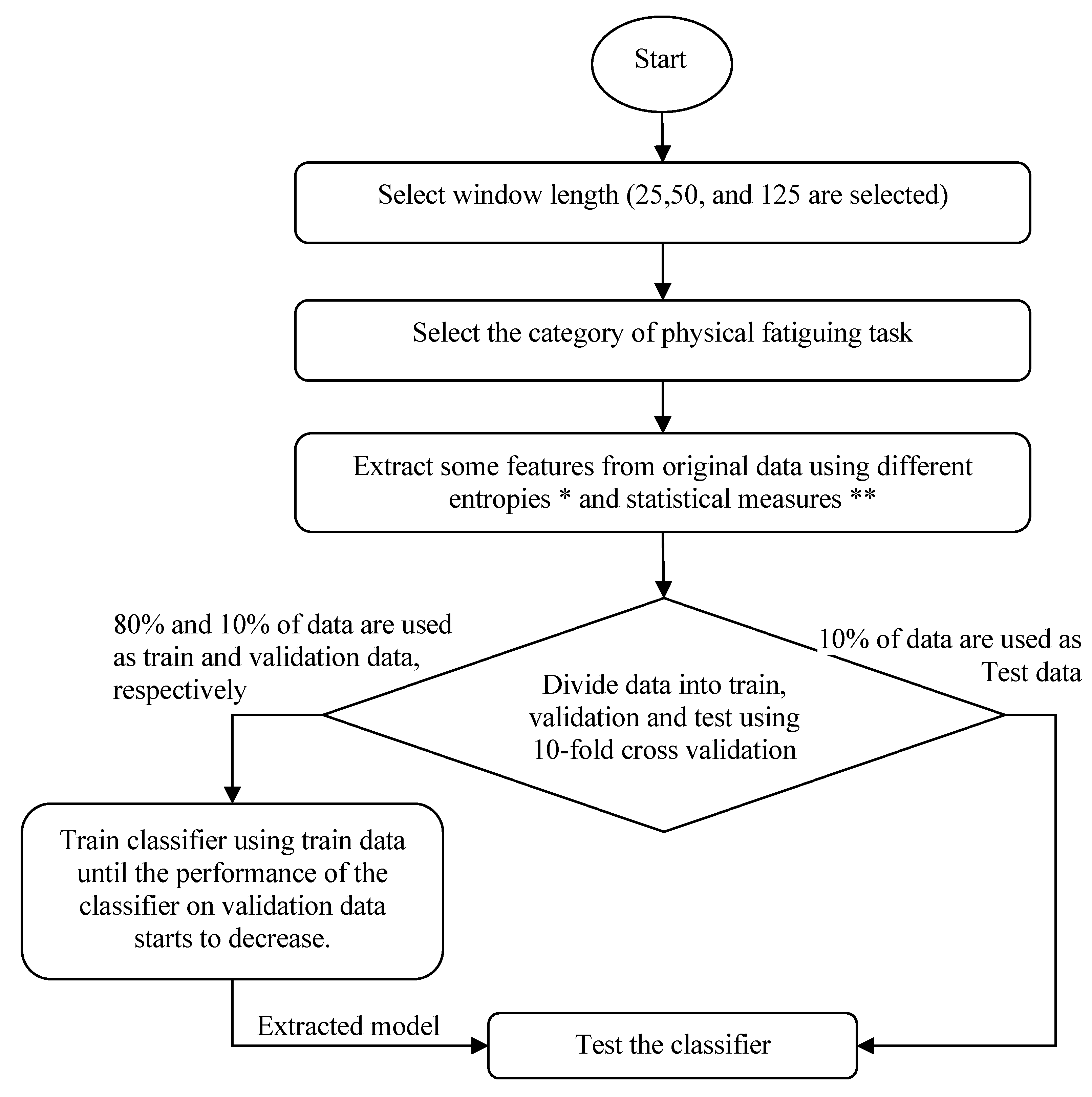
2.7. Proposed Method

In our proposed method, at first, we extracted 10 features in different conditions, such as different categories and window lengths, using different entropy methods, such as Shannon, Tsallis, Rényi, Log-Energy, and Kraskov, and statistical measures like mean, variance, standard deviation, kurtosis, and skewness. The window type was fixed. The different categories are ASM, MMH, and SPI. Meanwhile, the different window lengths used in this research were 25, 50, and 125 s. Then, the extracted data were divided into training, validation, and test sets according to ten-fold cross-validation. The training, validation, and test data were 0.8, 0.1, and 0.1 of the data in each fold. The classification algorithms were trained by the trained section of data. Overfitting was controlled by the validation data. Finally, the trained classification algorithms were tested based on the test data. The performance of the designed system was calculated by the mean of all folds. The flowchart of our proposed method is illustrated in Figure 1.

3. Experimental Results

To test the proposed method on the dataset collected from the eight subjects, we used three hours of heart rate signals of each subject. During these three hours, each subject may be fatigued at different points of time. In other words, a subject may feel fatigued several times during the three-hour test. The window size depends on the fundamental frequency, intensity, and changes of the signal [32]. Some of window sizes were tested to see which ones have more accurate results than others. The recorded heart rate signals were divided by window lengths of 25, 50, and 125 s. The overall number of data extracted from these samples is calculated as $\frac{8\ast 3\ast 3600}{\mathrm{window}\mathrm{length}}$. If the window length is 25, 50, or 125 s, we will have 3456, 1728, or 691 samples, respectively. This process will increase the number of samples and aids in making the application of machine learning algorithms in the manuscript strong. The labels of each of these samples are fatigued and non-fatigued. As the subjects’ states change and they may be fatigued or non-fatigued during the test, our data are balanced. For example, in the MMH category, when the window size is 25, there are 42.27% fatigued and 57.73% non-fatigued samples.

The nine best classification algorithms were tested on the extracted data in different sample rates for different categories of ASM, MMH, and SPI tasks. The window lengths that were used were 25, 50, and 125. Ten-fold cross-validation was used on the extracted data to evaluate the performance of the algorithms. We used the accuracy, sensitivity, specificity, and area under the curve (AUC) of the algorithms for their performance comparison [54,55,56]. The accuracy of these algorithms is shown in

Table 2. Accuracies (%) of different algorithms in various conditions.

	Sampling Rate
	25			50			125
Category Algorithm Name	ASM	MMH	SPI	ASM	MMH	SPI	ASM	MMH	SPI
KNN (K = 22)	84.67	72.2	57.32	86.67	73.4	59.82	86.57	73.27	58.67
KNN (K = 25)	84.84	72.05	57.49	87.06	73.23	59.69	86.56	73.71	60.50
Naïve Bayes	80.19	52.5	51.79	79.83	57.44	50.39	79.85	64.7	51.09
Decision tree	82.72	72.79	58.16	83.94	72.71	58.09	85.35	72.95	58.44
Random forest	83.72	74.89	60.16	84.17	74.79	62.09	86.6	75.95	60.44
Rule induction	85.66	75.44	61.19	86.67	75.61	61.34	87.76	79.67	71.97
Neural network	87.41	76.16	62.75	88.58	76.34	63.45	90.36	77.81	69.37
Linear regression	83.43	74.56	61.05	83.77	75.65	61.59	86.24	77.28	64.72
Logistic regression	82.87	72.77	58.31	82.69	75.82	58.78	82.78	77.71	59.2
LDA	84.15	74.58	60.79	85.63	75.52	61.72	87.63	77.28	66.01

. In this table, changing the color from green to red shows the gradient of the accuracy of the algorithms. The green color shows a lower accuracy level and the red color shows a higher accuracy level. According to this table, SPI accuracy is low, while ASM has a good accuracy rate.

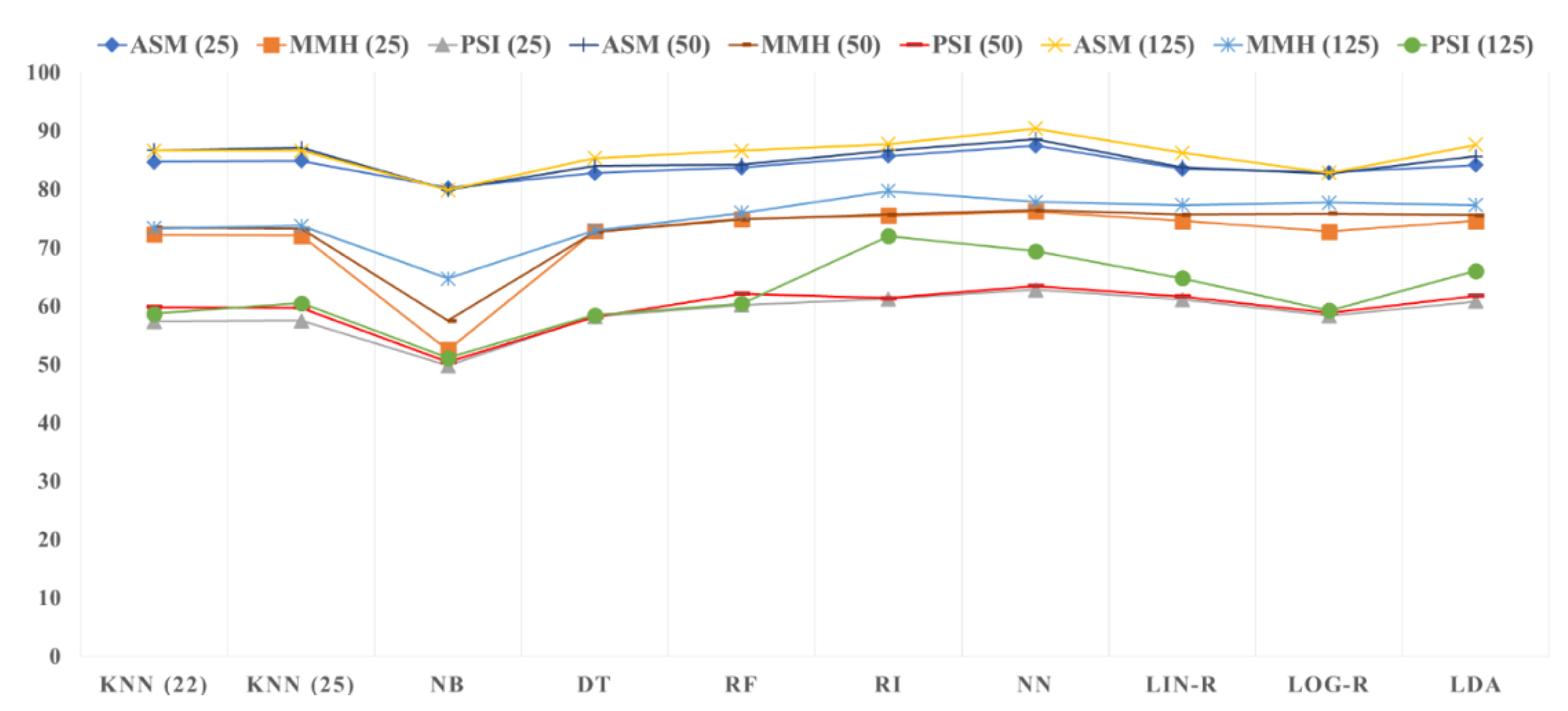
For a better comparison between different algorithms in various conditions, the accuracy of algorithms is also illustrated in Figure 2. It is clear in this figure that the neural network has the best performance in almost all tasks. We achieved the best accuracy (90.36%) in the ASM category and with a sampling rate of 125. In this category, the neural network, rule induction, linear discriminant analysis (LDA), random forest, and k-nearest neighbor with k equal to 22 had the accuracies of 90.36%, 87.76%, 87.63%, 86.6%, and 86.57%, respectively. We tested different values of K in the KNN algorithm. K = 22 and K = 25 showed the best performance. Linear regression’s performance is not very good because it is suitable for continuous domains, not discrete ones. In addition, Naïve Bayes had the worst performance in all conditions because it is only suitable for high-dimensional feature matrices (high number of features). In each category, when the sampling rate was decreased, the accuracy of algorithms also decreased. Overall, ASM had better performance with respect to the other categories.

As shown in Figure 2, ASM (125) has the best accuracy for almost all of the classifiers. ASM (50) and ASM (25) are in the second and third ranks, respectively. As shown, MMH and SPI have the second and third best performance after ASM. In each category, the greater the window length is, the better performance is achieved. However, the effect of the categories is more than that of the window length, i.e., the performance of MMH (125) is less than that of ASM (25).

The differences between some methods, such as KNN and LDA in ASM (25), are very small. Therefore, one method cannot gain superiority over another method in practice.

In

Table 3. Sensitivity (%) of different algorithms in various conditions.

	Sampling Rate
	25			50			125
Category Algorithm Name	ASM	MMH	SPI	ASM	MMH	SPI	ASM	MMH	SPI
KNN (K = 22)	69.62	48.79	55.33	61.21	54.18	58.18	64.65	53.2	56.93
KNN (K = 25)	77.38	55.05	54.86	64.97	59.9	55.51	67.8	59.2	58.92
Naïve Bayes	89.13	90.09	80.68	85.35	86.6	79.7	85.73	81.6	85.05
Decision tree	60.67	50.86	50.37	79.36	45.32	50.36	79.81	60.39	56.36
Random forest	62.53	55.49	55.65	75.28	50.38	61.43	68.99	65.52	58.52
Rule induction	66.88	72.89	57.12	70.84	68.17	59.53	73.46	62.95	71.09
Neural network	71.12	63.38	59.56	77.79	74.28	62.23	82.26	72.8	66.15
Linear regression	59.88	53.16	50.07	59.55	55.51	58.91	60.16	66.54	61.93
Logistic regression	51.12	45.97	58.8	60.25	57.26	53.1	51.26	62.8	58.12
LDA	56.75	53.01	56.56	59.87	54.24	55.6	62.08	66.4	59.58

, the sensitivity of the investigated algorithms is shown. Sensitivity, also called the true positive rate or recall, estimates the proportion of actual positives that are correctly recognized as such [57]. Similar to Table 2, changing the color from green to red shows the gradient of the sensitivity of the algorithms. The green color shows lower sensitivity, while the red color shows higher sensitivity. According to the results shown in this table, Naïve Bayes has the best sensitivity rate. The reason that this algorithm does not have a good accuracy rate while its sensitivity is high is that it is biased towards labeling the data as fatigue. This leads to a reduction in specificity and accuracy of the algorithm. The neural network and rule induction algorithms are in the second and third ranks, respectively. Meanwhile, logistic regression, linear regression, and KNN (K = 22) have the lowest sensitivity. To achieve the best performance of KNN, we changed K (number of nearest neighbors) from 1 to 50. When K was 22 and 25, the algorithm achieved the best accuracy rate. So, in this research, we used these two values for K in the KNN algorithm. As we only have 10 features, while the number of our records is 300, the neural network has better performance with respect to the KNN algorithm [58]. KNN sensitivity is low because the number of records with target features labeled as fatigue is less than non-fatigue records.

Table 4. Specificity (%) of different algorithms in various conditions.

	Sampling Rate
	25			50			125
Category Algorithm Name	ASM	MMH	SPI	ASM	MMH	SPI	ASM	MMH	SPI
KNN (K = 22)	86.16	88.44	73.14	96.13	88.06	75.43	89.63	88.13	70.56
KNN (K = 25)	85.8	85.89	80	95.82	85.68	69.92	89.53	88.5	69.44
Naïve Bayes	54.6	38.45	38.92	52.02	46.52	39.14	51.5	49.97	39.81
Decision tree	85.12	81.49	70.78	87.56	79.76	64.52	89.79	74.62	75.79
Random forest	89.11	83.42	74.72	89.37	80.49	75.38	91.29	80.59	77.42
Rule induction	88.76	83.87	75.93	94.3	85.86	69.68	94.9	89.91	72.59
Neural network	89.99	88.41	79.44	94.98	83.84	70.33	96.2	87.09	71.67
Linear regression	85.22	87.51	83.34	84.22	86.26	67.96	88.95	81.81	68.93
Logistic regression	86.95	89.97	79.63	85.84	80.46	68.96	85.74	83.07	79.07
LDA	88.22	87.6	85.42	88.48	82.55	70.57	94.43	83.14	84.81

shows the specificity of the different algorithms used in this research. Specificity is also called the true negative rate and estimates the proportion of actual negatives that are correctly recognized as such [54]. Again, the neural network has the best specificity rate, followed by rule induction, KNN (K = 22), KNN (K = 25), and LDA. KNN’s specificity is high because the number of records labeled as fatigue is much more than non-fatigue records. So, it tends to classify records as non-fatigue. Meanwhile, according to this table, Naïve Bayes has the worst specificity rate. According to this table, SPI specificity is low, while ASM has a good specificity rate. In

Table 5. Area under the curve (AUC) of different algorithms in various conditions.

	Sampling Rate
	25			50			125
Category Algorithm Name	ASM	MMH	SPI	ASM	MMH	SPI	ASM	MMH	SPI
KNN (K = 22)	0.82	0.78	0.74	0.85	0.77	0.69	0.86	0.81	0.72
KNN (K = 25)	0.79	0.65	0.72	0.84	0.79	0.76	0.87	0.84	0.81
Naïve Bayes	0.77	0.79	0.71	0.81	0.8	0.74	0.79	0.8	0.79
Decision tree	0.87	0.81	0.74	0.88	0.87	0.82	0.91	0.89	0.81
Random forest	0.83	0.78	0.71	0.86	0.83	0.82	0.89	0.85	0.83
Rule induction	0.84	0.81	0.76	0.84	0.81	0.79	0.89	0.83	0.8
Neural network	0.83	0.79	0.79	0.88	0.84	0.78	0.88	0.87	0.86
Linear regression	0.84	0.79	0.73	0.86	0.8	0.72	0.89	0.8	0.79
Logistic regression	0.79	0.76	0.77	0.84	0.81	0.78	0.86	0.83	0.73
LDA	0.86	0.83	0.81	0.89	0.89	0.83	0.92	0.89	0.88

, the AUC can be seen for different algorithms.

The AUC measures the tradeoff between true positive rate and false positive rate. As the threshold varies over all possible values, the AUC is an evaluation of the classifier. It is a metric that checks the quality of the value generated by a classifier and then compares it to a threshold. It does not test the quality of a specific threshold value [58]. According to Table 5, ASM (125) has the best AUC in almost all of the classifiers. According to the AUC values, LDA, decision tree, and neural network have the best performance, respectively.

The ranking of features in different tasks is shown in

Table 6. The rankings of features in different categories when window length is 25.

25-ASM		25-MMH		25-SPI
Feature Name	Weight	Feature Name	Weight	Feature Name	Weight
Shannon entropy	1.0	Shannon entropy	1.0	Shannon entropy	1.0
Standard deviation	0.9703	Standard deviation	0.9382	Standard deviation	0.9937
Log-Energy entropy	0.9624	Log-Energy entropy	0.8563	Log-Energy entropy	0.9935
Kraskov entropy	0.4774	Rényi entropy	0.3515	Kraskov entropy	0.3784
Variance	0.4774	Tsallis entropy	0.3487	Variance	0.3784
Rényi entropy	0.4211	Kraskov entropy	0.3387	Skewness	0.2665
Skewness	0.0867	Variance	0.3387	Rényi entropy	0.1909
Kurtosis	0.0818	Skewness	0.1176	Tsallis entropy	0.1693
Tsallis entropy	0.0789	Kurtosis	0.0088	Kurtosis	0.0136
Mean	0.0	Mean	0.0	Mean	0.0

,

Table 7. The rankings of features in different categories when window length is 50.

50-ASM		50-MMH		50-SPI
Feature Name	Weight	Feature Name	Weight	Feature Name	Weight
Standard deviation	1.0	Shannon entropy	1.0	Shannon entropy	1.0
Shannon entropy	0.9984	Standard deviation	0.9287	Log-Energy entropy	1.0
Log-Energy entropy	0.9828	Log-Energy entropy	0.8926	Standard deviation	1.0
Kraskov entropy	0.4981	Kraskov entropy	0.4087	Kraskov entropy	0.7753
Variance	0.4981	Variance	0.4087	Variance	0.7753
Rényi entropy	0.4185	Tsallis entropy	0.3964	Rényi entropy	0.5393
Skewness	0.2212	Rényi entropy	0.3854	Tsallis entropy	0.4087
Kurtosis	0.1799	Skewness	0.2306	Skewness	0.2253
Mean	0.1687	Kurtosis	0.0309	Kurtosis	0.1042
Tsallis entropy	0.0	Mean	0.0	Mean	0.0

and

Table 8. The rankings of features in different categories when window length is 125.

125-ASM		125-MMH		125-PSI
Feature Name	Weight	Feature Name	Weight	Feature Name	Weight
Log-Energy entropy	1.0	Log-Energy entropy	1.0	Shannon entropy	1.0
Standard deviation	1.0	Standard deviation	1.0	Standard deviation	0.8883
Shannon entropy	0.9942	Shannon entropy	0.9942	Log-Energy entropy	0.8118
Kraskov entropy	0.4857	Kraskov entropy	0.4857	Tsallis entropy	0.4038
Variance	0.4857	Variance	0.4857	Rényi entropy	0.3942
Rényi entropy	0.3420	Rényi entropy	0.3420	Kraskov entropy	0.3695
Skewness	0.2744	Skewness	0.2744	Variance	0.3695
Mean	0.2594	Mean	0.2594	Skewness	0.2287
Kurtosis	0.2108	Kurtosis	0.2108	Kurtosis	0.0016
Tsallis entropy	0.0	Tsallis entropy	0.0	Mean	0.0

. In these tables, when the weight of a feature is high, it shows that this feature is more valuable in the classification of that record. Different feature selection algorithms have been suggested. We used one of the best algorithms, namely information gain [56,59,60]. According to the results shown in these tables, when window length was changed, different weights were assigned to features. As these tables show, in comparison with statistical measures, entropies commonly have better ranks in the classification of fatigue. For example, Shannon entropy is the best feature in six cases out of nine. Log-Energy entropy also has a high rank. Among the statistical measures, the standard deviation has a good rank. It has one first-place rank and seven second-place ranks according to these tables. Among statistical tests, mean has the worst rank, and among entropies, Tsallis entropy has the worst rank. Skewness and kurtosis usually do not have good ranks.

Discussion

In our research, the physiological data collected by Maman et al. [22] were used to detect workers’ physical fatigue. They used five different sensors’ features in their research. However, in this research, only the data extracted from the heart sensor were used. Many studies have demonstrated the advantages of entropy over conventional methods [28]. In contrast to Maman et al. [22], whose research which used only statistical measures, entropies are used in our proposed method. According to the achieved results, entropies are better than statistical measures for fatigue detection. In addition, ten-fold cross-validation was used in the proposed method to estimate the performance of the system. Maman et al. [22] used six out of eight cases for training the algorithms and the rest for testing. The most important weakness of the work of Maman et al. is that the accuracy of their proposed algorithm is not reported due to the small sample size. In addition, in contrast to Maman’s proposed method, in this research, we applied some of the frequently used classification algorithms. Using these powerful feature extraction and classification algorithms, we achieved the same results using the data prepared by only one sensor, while they used data of five sensors.

The results show that the extracted features of data have a significant influence on the accuracy of algorithms for fatigue detection. Some features such as standard deviation, Shannon entropy, and Log-Energy entropy have a high rank in feature selection algorithms. So, they can help classification algorithms a lot. An interesting point is that statistical measures have lower ranks with respect to entropies. Only the standard deviation has a good rank among statistical measures. Meanwhile, Tsallis entropy has the lowest rank between different entropies. Another interesting point is that in the ASM category, the algorithms can classify fatigue better than in MMH, and in the MMH category, classification can be done more precisely than in the SPI category. In addition, the greater the window length is, the better performance of the algorithms is achieved. Among the investigated algorithms, the neural network, rule induction, LAD, and KNN have good performance in fatigue detection.

Based on the achieved results, it is concluded that using entropies instead of or alongside statistical measures can improve the performance of diagnosing systems, such as fatigue detection. Moreover, using heart rate as the only indicator for fatigue assessment provided two benefits toward real-time detection of fatigue in the workplace. First, it is not required for the workers to wear several sensors. Second, since a lower amount of data is required to be processed, time and cost savings are achieved by using heart rate as the only sensor for fatigue detection.

The current findings are, however, subject to certain limitations. Specifically, the sample size used by the source publication [22] was small and, therefore, individual variation between participants (e.g., age, height, body mass) can skew the results. In future research, we suggest collecting more data to account for individual variation and to add greater generalizability to the more accurate predictions generated by our new analysis method.

4. Conclusions and Future Work

In this research, for fatigue detection, some important features were extracted from heart signals using entropies and statistical measures. The frequently used classification algorithms were applied to test the performance of the proposed method. Neural networks and rule-based induction could achieve excellent results in our tests. Overall, entropies extracted better features for classification in comparison with statistical measures.

It was shown that the proposed method provides an efficient tool for accurate and real-time monitoring of physical fatigue, aids in enhancing workers’ safety, and prevent accidents. The proposed method can be useful for developing warning systems against high levels of physical fatigue and designing better resting times to improve workers’ safety. Future research can utilize the proposed method in a user-friendly application to conduct this analysis so that project managers can look at workers’ fatigue in real time with a reliable accuracy.

Collecting more data can result in more accurate results. In future research, a larger dataset can be collected to improve accuracy and increase generalizability. As features play a vital role in the performance of an algorithm, extracting new features using other entropies may help to improve our proposed method’s accuracy. According to the achieved results, neural networks showed outstanding performance for fatigue detection. Therefore, deep learning algorithms provide a new horizon in this direction for future research.