CityScapeLab Berlin: A Research Platform for Untangling Urbanization Effects on Biodiversity
by
 ,
,
Moritz von der Lippe
1,2,* ,
,
Sascha Buchholz
1,2,
Anne Hiller
1,2,
Birgit Seitz
1,2 and
Ingo Kowarik
1,2 1
Department of Ecology, Technische Universität Berlin, D-12165 Berlin, Germany
2
Berlin-Brandenburg Institute of Advanced Biodiversity Research (BBIB), D-14195 Berlin, Germany
*
Author to whom correspondence should be addressed.
Sustainability 2020, 12(6), 2565; https://doi.org/10.3390/su12062565
Submission received: 2 March 2020
/
Revised: 19 March 2020
/
Accepted: 20 March 2020
/
Published: 24 March 2020
(This article belongs to the Special Issue Biodiversity Conservation and Sustainable Urban Development)
Abstract
:Urban biodiversity conservation requires an understanding of how urbanization modulates biodiversity patterns and the associated ecosystem services. While important advances have been made in the conceptual development of urban biodiversity research over the last decades, challenges remain in understanding the interactions between different groups of taxa and the spatiotemporal complexity of urbanization processes. The CityScapeLab Berlin is a novel experimental research platform that allows the testing of theories on how urbanization affects biodiversity patterns and biotic interactions in general and the responses of species of conservation interest in particular. We chose dry grassland patches as the backbone of the research platform because dry grasslands are common in many urban regions, extend over a wide urbanization gradient, and usually harbor diverse and self-assembled communities. Focusing on a standardized type of model ecosystem allowed the urbanization effects on biodiversity to be unraveled from effects that would otherwise be masked by habitat- and land-use effects. The CityScapeLab combines different types of spatiotemporal data on (i) various groups of taxa from different trophic levels, (ii) environmental parameters on different spatial scales, and (iii) on land-use history. This allows for the unraveling of the effects of current and historical urban conditions on urban biodiversity patterns and the related ecological functions.
1. Introduction
Biodiversity loss and ongoing urbanization are coinciding global trends in the Anthropocene [1] that challenge the future of biodiversity and the multiple benefits that urban nature provides for urban residents [2,3,4]. While urban growth often conflicts with biodiversity conservation in adjacent natural areas [5], cities can harbor surprisingly high biological diversity [6,7,8], including endangered species [9,10,11]. In an era of accelerating urbanization, developing biodiversity–friendly cities is needed to combat the global biodiversity crisis—and is consequently on the urban agenda [12,13,14]. Importantly, positive relationships between biodiversity and ecosystem services have been increasingly evidenced [4,15,16,17], and thus biodiverse urban systems are also a prerequisite of urban sustainability due to the wealth of associated ecosystem services [2,18].
Urbanization exerts a multitude of changes to the environment driven by human activities that induce often rapid changes to urban land-use types [19]. Cities are coupled socioecological systems [20,21,22], which are characterized by interconnections between the urban form with its built structures and the socioeconomic and ecological features of urban systems [20,22,23] (Figure 1). How these changes modify urban biodiversity patterns—and the associated benefits for urban residents—is a key question for understanding the potential contribution of urban biodiversity to livable cities and biodiversity conservation.
Besides human activities, natural landscape factors also impact on urban biodiversity. The geomorphological richness of areas where cities were formerly established [24], or the existence of natural remnants within cities [10,25], significantly contribute to the biological richness of many cities. In the same vein, anthropogenic ecosystems can support urban biodiversity, with a myriad of ecological niches, involving habitat analogs to natural systems as well as novel urban ecosystems [26,27]. Urban biodiversity has, from early on, been shown to reflect major patterns of urban land use and the associated human agency. Previous studies revealed the relevance, for example, of settlement size [28,29,30], spatial differentiation of the urban form [6,30,31], the identity of biotope types [32,33,34], the position of habitats along urban‒rural gradients [35,36,37], or human mobility patterns [38,39].
Yet, despite the broadly acknowledged biological richness of cities there is also a “dark side” of urbanization, putting urban biodiversity at risk by different processes: local extinctions [40,41], establishment failures [10], population decline [42], and shifts in the (functional) composition of urban species assemblages [43,44]. Shwartz et al. [45] thus conclude from their meta-analysis that the contribution of cities to the conservation of the world’s biodiversity is still ambiguous.
Given the multi-faceted and multi-directional effects of urbanization on urban nature, a key question for developing sustainable and biodiverse cities is how different urbanization drivers translate to opportunities or challenges for urban biodiversity in general, and for different groups of species in particular. Despite important insights from a wealth of recent urban biodiversity studies [8,45,46] and advanced research strategies, e.g., [47], some major challenges remain in understanding the complex interactions between urbanization and biodiversity. Most challenging are the eminent heterogeneity and temporal dynamics of ecological and socioeconomic patterns in cities that are likely unparalleled in other types of ecosystems [19,48]. As a consequence, ecological research in urban settings has to untangle multi-faceted relationships between urbanization and biodiversity in relation to urbanization parameters (e.g., the population density, impervious surface, and fragmentation) and biodiversity components (e.g., taxonomical and functional groups, endangered species, and ecosystem types).
To inform urban biodiversity conservation, here we present the conceptual and methodological approach of the CityScapeLab Berlin as a new, integrative, and flexible research platform for an enhanced understanding of the interconnections between urbanization and biodiversity in metropolitan regions (Figure 1). The CityScapeLab Berlin was conceptualized in the context of the Berlin-Brandenburg Institute of Advanced Biodiversity Research (BBIB), which is a consortium of university and non-university research institutions working on biodiversity research located in Berlin and Potsdam (see https://www.bbib.org/home.html). Shortly after, the implementation of the CityScapeLab in the real world started in 2016, funded by the German Federal Ministry of Education and Research (BMBF) within the collaborative project “Bridging in Biodiversity Science—BIBS” and led by the Technische Universität Berlin. The research infrastructure of the CityScapeLab is used by a suite of cross-disciplinary partners of the BIBS consortium and supplements other ScapeLabs that are being established in the rural landscape outside Berlin, i.e., the AgroScapeLab and the LakeScapeLab (see https://www.bbib.org/scapelabs.html).
The major aim of the CityScapeLab Berlin is to provide a flexible research platform for
- exploring the effects of urbanization and rapid transitions in urban land-use patterns on biodiversity and ecosystem functioning at different spatial and temporal scales;
- developing and testing theories on the intersection between urbanization and biodiversity;
- supporting policies on the integration of biodiversity and the associated ecosystem services into urban landscapes, as a contribution to sustainable, livable, and resilient cities.
In the following, we first present the principal approach of the CityScapeLab, which was developed in response to the aforementioned key challenges to urban biodiversity research (Section 2). Second, we explain the suitability of the Berlin metropolitan region for urban biodiversity studies and links between the approach of the CityScapeLab and the long tradition of urban ecological research in Berlin (Section 3). Third, we specify the methodological approaches in more detail to support traceability and comparability with other approaches (Section 4). Finally, we give a brief outlook on the possible further development of the CityScapeLab and on the implications for biodiversity research and conservation in cities worldwide.
2. Fundamental Approach of the CityScapeLab Berlin
In the following, we present five key components that underlie the approach of the CityScapeLab Berlin to the major challenges in urban ecology studies. These are the focus on a model ecosystem and the bridging of scales in regard to space and time (Figure 2) as well as for organisms and ecological novelty.
2.1. Model Ecosystem
The complexity of urban areas with a fine-grained mosaic of land-use types is unparalleled in most non-urban landscapes [48]. While the complexity of the urban matrix can be well incorporated into modern patch-matrix frameworks [49], urban ecological research is confronted with a large heterogeneity between potential study objects. This complexity represents a major challenge because biodiversity responses to urbanization are strongly context dependent. The type of urban land use (or biotope, habitat, ecosystem), for example, is a key predictor for biodiversity patterns in cities [30,34,50], and these are further modulated by variation within the same land-use type such as the patch size or socioecological features [46,50,51,52].
The CityScapeLab Berlin, thus, sets a focus on a standardized type of model ecosystem to unravel the urbanization effects on biodiversity from the effects that would otherwise be masked by different land-use types or distinct site conditions. As a first model ecosystem, we selected extensively managed dry grassland (henceforth “urban grassland”) due to the following reasons:
- ■
- ■
- Urban grassland patches are usually subject to a varying intensity of anthropogenic recreational activities associated with trampling, soil disturbance, or nutrient influxes—or they exist without such interferences, e.g., in conservation areas;
- As a low productivity ecosystem, urban dry grassland is particularly sensitive to nutrient influxes from the urban matrix or from local human activities [63];
- Urban grassland is often invaded by alien plant species [57,67] as is the urban dry grassland in Berlin, with an average proportion of 25% of alien species [68]. Grassland, as a shared habitat of many native and alien species, allows analyses of multiple biotic interactions (e.g., native‒alien, plant‒animal, or belowground‒aboveground interactions);
- Urban grassland has a limited structural heterogeneity due to the prevalence of grasses and herbs and a similar management intensity on low productivity sites—dry grassland in Berlin, for example, is usually mown up to two times a year, or less;
- Urban grassland often spans a large gradient of ecological novelty, from near-natural sites to designed greenspaces to novel ecosystems on vacant land [66], encompassing sites with natural and anthropogenic soils and including patches with different land-use legacies and current or historical habitat connectivity [61].
Selecting urban grassland as model system for the CityScapeLab Berlin allows enhanced insights into the intersection of urbanization and biodiversity by reducing environmental heterogeneity. Furthermore, urban dry grassland allows for the untangling of urbanization effects from other biodiversity drivers. In the future, this approach can be complemented by other important types of urban ecosystems such as forests, ponds, green roofs, or gardens.
2.2. Bridging Spatial Scales
How urbanization modulates urban biodiversity patterns is complex. Manifold features of urban form and related drivers, mechanisms, and socioecological consequences influence biodiversity [21,69]. While early urban ecological work often studied biodiversity patterns by comparing cities and their rural environments, e.g., [24] or by analyzing urban to rural gradients [36], a predominant line of progression was the differentiation and more exact measurement of urbanity and its components from spatially explicit communal datasets. This has resulted in an increasing number of urbanity measures and landscape parameters in urban studies [70,71].
Yet, urbanization drivers operate at different scales, e.g., from local recreational pressures, to impacts from the urban matrix, including pressures from the neighborhood (e.g., the effects of street lighting) up to the city scale (e.g., urban heat island). Related biodiversity effects differ correspondingly because their importance, or even the direction of their ecological impact, varies with the spatial scale on which they are studied [72]. Ultimately, the spatial scale also matters for taxa that are potentially subject to urbanization drivers because urban biodiversity components starkly differ in their radius of activity, from soil biota to bats, birds, or large mammals such as wild boars that can move on a regional scale [73]. Urban biodiversity research, thus, needs to bridge spatial scales [74].
An important goal of the CityScapeLab Berlin is, therefore, to create a flexible research infrastructure that allows the bridging of spatial scales in urban biodiversity research with regard to both urbanization drivers and potentially affected organisms. This is being achieved by linking spatial scales from local to regional scales (Figure 1):
- The basic survey units of the CityScapeLab are patches of the selected model ecosystem, i.e., grassland patches. These share a rather homogeneous vegetation structure but usually differ in size, adjacency to other, and connectivity to similar ecosystems. A minimum patch size of 100 m² still ensures that biodiversity measurements of taxa of different spatial range can be linked to each other and the grassland patch. For example, measures of bat activity from an automated bat recorder usually cover a radius between 12 and 75 m but can still be reasonably related to light traps of nocturnal insects of the same patch. Moreover, this patch-centered approach allows for analyses of biotope transitions at the edge to surrounding habitats and different land uses;
- Each urban grassland patch encompasses one randomly located plot with a standardized size (4 × 4 m) for sampling environmental variables and some taxa at the plot scale (e.g., plants and arthropods). Other taxa, including grasshoppers, can be sampled along transects at the patch level, spatially linked with the plots or by nearby exposed camera traps;
- Next to the plot and within the patch, an area is foreseen where destructive investigations (e.g., biomass measurements e.g., [63]) or experiments can be performed (e.g., plant-pollinator interactions [75]). While the plots remain undisturbed, results from the adjacent experimental area can be related to the environmental variables measured at the plot or patch level;
- A range of environmental and socioeconomic data is available for spatial buffers in the surroundings of the patches thus allowing us to elucidate relationships between the urban matrix and the biodiversity patterns at the plot or patch scale;
- To ensure analyses of functional spatial relations between the plot or patch scale, the city area, and the surrounding countryside, the research platform not only covers the entire metropolitan region of Berlin but also includes typical rural landscapes within a buffer of approximately ten kilometers beyond the administrative borders of Berlin (Figure 3). Results from the biodiversity analyses, thus, can be synthesized, or differentiated, on a regional scale. Citywide spatial data sets on all significant environmental and urbanization effects enable the linking of the local and supra-local level to regional drivers of biodiversity;
- In parallel, biodiversity analyses from the study sites can be related to data at higher spatial scales. For few taxa, grid-based data exist in Berlin (e.g., for vascular plants [76]), while total species inventories are available for a broad range of plant and animal groups on the city scale. As these are often coupled with Red Lists of species endangered or extinct in Berlin (Table 1), biodiversity responses to urbanization can be specified for species of particular conservation concern.
2.3. Bridging Temporal Scales
Cities around the world differ in their historical background, for example, in age or the inclusion of differently old remnants of natural or cultural landscapes within the city borders. Such differences matter for the soil characteristics [77] and for biodiversity features. Local extinction rates, for example, differ in cities with contrasting historical background [40]; city age is a good predictor for bird diversity [78].
Within a given city, the current land-use patterns usually encompass transformation stages from natural remnants to novel urban ecosystems [19,27]. As a consequence, the same urban ecosystem type can strongly differ in regard to the habitat continuity (age since establishment), current versus historical habitat connectivity [79], or ecological novelty [80,81]. The importance of human and other legacies for explaining current biodiversity patterns in cities has been convincingly demonstrated [61,82,83] and, consequently, the need to integrate the temporal dimension in urban studies [19].
Yet, most urban ecology research still relies on “snapshot studies” and rarely includes historical layers in the analyses, with few exceptions [82,83]. Long-term studies on the succession of urban ecosystems are limited but see [84,85]. The two urban long-term ecological research (LTER) sites in Baltimore and Phoenix, US, have offered the opportunity of time series analyses since the 1990s [86]. These unique data demonstrate, for example, that it is not only change in urban structure that drives change in biodiversity and ecological processes but also the temporal socioeconomic dynamics [87].
The CityScapeLab Berlin integrates the historical dimension as follows:
- For the total area of Berlin, the historical land use for the settlement area, woodland, and grassland has been traced back from analyses of georeferenced historical maps from three periods of time since the beginning of the 19th century. This allowed for the incorporation of both “old” grassland patches (established more than 100 years ago) and “new” grassland patches (established since 1945) into the set of survey areas. This enables testing for the relevance of land-use continuity and for habitat connectivity at different periods of time for current biodiversity patterns;
- All study areas were established as permanent monitoring sites, with a plot precisely mapped at centimeter accuracy, allowing for the temporal dynamics in biodiversity patterns and processes to be captured in the future. Some of the established monitoring plots overlap with previous vegetation surveys, dating back between 10 and 30 years. These data well support historical comparisons because they were georeferenced at sub-meter accuracy;
- Ultimately, the survey patches also stretch along a gradient of ecological novelty, both in terms of biotic novelty and abiotic novelty. As illustrated by Figure 4, the patches span from sites with near-natural soils (e.g., grassland in a forest or agricultural context), to areas with anthropogenic soils (e.g., in historical parks), to novel sites with artificial soils, such as in transportation corridors (e.g., motorway embankments), or vacant land (e.g., abandoned rail yards). This allows for the unraveling of the relationships between different levels of ecological novelty and ecological and evolutionary patterns in urban environments—with significant implications for conservation strategies in the face of global change [80,81].
2.4. Bridging Taxonomical and Functional Groups
Different groups of animals and plants respond differently to urbanization [46,74,88] as do different functional groups [43,89]. Yet, multi-taxon analyses are rare [74,89], and some groups of taxa (e.g., birds and vascular plants) are overrepresented in urban studies [36,45]. Seibold et al. [89], thus, not only argue for multi-taxon studies, but for integrating different trophic levels in multi-trophic studies. It is, therefore, an important challenge to unravel the effects of urbanization on a wide range of taxonomic and functional groups. While many early biodiversity studies relied largely on species richness, a range of diversity measures, including functional diversity, can be used for testing for urbanization effects on a comprehensive set of biodiversity components and the related ecological processes and ecosystem services [63,90,91]. A further deficit is the understanding of complex biotic interactions in urban contexts e.g., [92] that can be significantly modulated by urbanization [75,92,93].
The CityScapeLab platform supports studies in multi-taxa and multi-trophy systems under the influence of various urban stressors:
- The focus on a standardized ecosystem type allows for the identification of the relative importance of urbanization drivers versus local environmental conditions in shaping community assembly and modulating biotic interactions;
- The multi-scale approach (see Section 2.2) provides a flexible research infrastructure to incorporate taxa with starkly varying activity radii into the analyses. Thus, different taxa representing different trophic levels can be analyzed with regard to urbanization responses in terms of biodiversity measures and biotic interactions;
- Dry grassland as a species-rich model ecosystem is ideal for investigating a large variety of interactions as most trophic levels are represented by different taxonomic groups with a potentially large number of native and alien species.
2.5. Integrating the Human Dimension
Reflecting the nature of cities as socioecological, i.e., coupled human and natural systems [21,22], several studies explicitly incorporate parameters related to human agency, either by assessing the overall human impact (the hemeroby approach [94,95]) or by relating single socioeconomic features to urban biodiversity patterns [20,46,96]. The latter has mainly been done indirectly by analyzing spatially explicit socioeconomic datasets as predictors of biodiversity patterns (e.g., the socioeconomic neighborhood status [96,97]). Research that integrates direct measures of human activities on the local scale are scarce though. Exceptions are studies on cultivated plant species as a result of human preferences and triggers for plant invasions [98,99] or on feedback between the management and ecosystem features of urban grassland [100,101].
While ecological research has demonstrated the importance of different dimensions of human agency for understanding urban biodiversity, there is still a need for comprehensive quantifications of the human impact. Beyond this background, the CityScapeLab Berlin combines indirect and direct measures of human impact:
- The study areas are intentionally not fenced in to allow analyses of a wide range of everyday interactions of city dwellers with the grassland;
- On a neighborhood level, relationships between biodiversity patterns and human influences can be elucidated by incorporating socioeconomic biodiversity predictors. High-resolution spatial data on socioeconomic features are available from the Berlin Social Atlas on the basis of neighborhoods that cover on average 7500 inhabitants. Further spatial data on environmental justice make it possible to address citizens not only as drivers of ecological change but also as those affected by environmental pressures in the city;
- Free access to the research sites also allows the application of methods from the social sciences, for example, observations of the behavior of humans staying on or passing through the study plots [102].
3. Study Region and Linkages to Urban Biodiversity Research
3.1. Berlin as a Model of a Metropolitan Region
Berlin is Germany’s largest city, with 3.6 million inhabitants within a total area of 891.1 km2. Berlin is a historical city with roots reaching back to the medieval times. Unlike many other historical cities, however, today’s Berlin has a polycentric structure with a range of differently aged urban nuclei. Urbanization in this area started from four medieval centers, the cities of Köpenick, Spandau, Berlin, and Cölln, which received their municipal charters around 1200 AD; Charlottenburg was established as a baroque city foundation in 1705. In addition, a large number of villages have emerged since the Middle Ages. In the wake of rapid industrialization and Berlin’s designation as the German capital in 1871, the population grew rapidly from circa 424,000 inhabitants in 1849 to four million inhabitants in 1925. This led to numerous expansions of the existing urban centers and the founding of new cities at the expense of rural settlement and landscape elements. In 1920, today’s Berlin was founded as a union of eight cities, 59 villages, and 27 manor districts. The resulting polycentric urban structure is closely interwoven with numerous remnants of the natural landscape (forests, rivers, lakes, and wetlands) and the preindustrial cultural landscape (agricultural fields and grassland and forest plantations), which are located between individual settlement cores and on their outer edges. In addition to the typical elements of designed green spaces within the built areas (parks, gardens, cemeteries, etc.), a new type of open space emerged after the Second World War due to the sharp decline in population and a slow urban development until German reunification in 1989. Natural revegetation of vacant land and abandoned areas of transport infrastructure led to a novel type of urban wilderness [103]—as with many other cities that shrink in the wake of political or economic transformation.
In terms of land use, about 59% of Berlin’s surface is dominated by built-up areas and streets; green and blue spaces cover 41% of the area, including forests (18%), lakes and rivers (6%), parks (6%), allotment gardens (5%), fields (5%), and meadows (1%) [104]. Sandy and loamy soils from the last ice age prevail in the (near-) natural landscapes while strongly modified, anthropogenic soils are associated with different urban land-use types. While the natural vegetation in the Berlin region is dominated by deciduous forests and wetlands, grasslands here represent—with very few exceptions—anthropogenic vegetation types, shaped by mowing or grazing and covering agricultural sites, urban green spaces, transportation corridors, and vacant land [105]. Dry grassland as a sub-type of extensively managed grassland (i.e., without fertilization or irrigation) historically emerged in pastured woodland on sandy soils and in pastures as subsequent degradation stages [106]. Today, some of these patches still exist in Berlin in the context of forest or agricultural land. Yet, the largest patches of dry grassland are associated with old parks and airfields in the city [54]; many smaller patches are integrated into various urban land-use types (Figure 3a). As a special feature, many patches of dry grassland have developed on the former frontier line where the Berlin wall delimited East and West Berlin. This unique linear structure was later developed as a green belt [107] and largely preserved as open land, allowing the study of inner-city dry grasslands with high connectivity between habitat patches.
Berlin’s climate is temperate, with an annual average temperature of 9.9 °C and a mean annual precipitation of 576 mm, measured by an inner-city weather station in the observation period of 1981–2010. Within this period, Berlin increasingly experienced periods of higher temperatures and less precipitation [108]. Local temperatures are significantly modulated by the urban form, with mean temperature values increasing with the surface of buildings adjacent to weather stations [109]. The book on the urban ecology of Berlin by Sukopp [105] provides comprehensive insights into the vegetation, fauna, soils, and climate and history of Berlin. Spatially explicit data on many facets of Berlin’s socioecological features are accessible online in the Berlin Environmental Atlas (https://www.stadtentwicklung.berlin.de/umwelt/umweltatlas/ework.htm).
Today Berlin represents not a single city but a metropolitan region that within its administrative boundaries encompasses several previously independent cities, rural settlements, and a range of (near-) natural landscape remnants. The development of Berlin’s built, green, and blues areas was often spatially and temporally undirected and evolved at very different paces, including periods of (sometimes coinciding) rapid growth or shrinking. Berlin is, thus, a model region for comprehensive analyses of various urbanization impacts on biodiversity at a regional scale.
3.2. Links to Research Traditions in Berlin
The CityScapeLab Berlin and the studies conducted within it benefit from two traditional lines of research in Berlin: the tradition of natural history and the work of the so-called “Berlin School of Urban Ecology”. As in many central European cities (e.g., Halle [41]), there is a wealth of research on flora and vegetation in Berlin in the tradition of natural history, going back some 400 years [110,111]. This has resulted in a series of accurate floristic inventories, from the floras of Johann Sigismund Elssholtz, Carl Ludwig Willdenow, and Paul Ascherson to the current Atlas of the Berlin Flora by Seitz et al. [76]. These historical sources informed a Red List of extinct and endangered plant species in Berlin in 1974—probably the first for a large city. Since 1982 such Red Lists are also available for many animal groups and have been updated several times for a range of taxa (most recently Seitz et al. [112] for plants).
Far beyond the tradition of natural science, Berlin has played a “pivotal role for the early emergence of urban ecology“ [113]. This is mainly due to research in the context of the “Berlin School of Urban Ecology”, which was founded by Herbert Sukopp at the Institute of Ecology of the Technische Universität Berlin around 1970 [114]. In a first phase of related work, one main focus was on analyzing biodiversity patterns and biotope types across all land-use types—from near-natural to novel urban ecosystems—describing species’ compositions and relationships to different features of the urban form and highlighting the importance of urban nature for biodiversity conservation. This work has been summarized in an edited book [105]. In recent years, the focus of the work in Berlin has moved to a more mechanistic understanding of the urban biodiversity patterns and underlying drivers and to human‒nature interactions.
The previous work in Berlin was valuable for the establishment of the CityScapeLab in several ways—(1) by providing reference bases for biodiversity at the level of the city as a whole, such as total species inventories or the proportion of endangered species for different groups of plants and animals; (2) by enabling historical comparisons as some of the study sites investigated several decades ago could be integrated into the current research network; and (3) by supporting the refinement of research hypotheses, because the importance of some predictors of biodiversity patterns has already been elucidated.
4. Methodological Approaches
4.1. Dry Grassland Survey Areas
To establish the network of grassland survey areas, as a first step a stratified random selection from all potential dry grassland patches in the metropolitan area of Berlin was carried out. Using the digital biotope maps of Berlin and Brandenburg, we preselected all biotope patches that were attributed to the biotope code 05120 (i.e., dry grasslands [115]). In terms of the phytosociological vegetation classification (Braun-Blanquet approach [116]) all selected plots belong to plant communities of the Sedo-Scleranthetea Br. Bl. 1955 em. Th. Müll. 1961 [106,117]. The characteristic and most frequent species included the grasses Agrostis capillaris and Festuca brevipila, and the herbs Cerastium semidecandrum, Potentilla argentea, Rumex acetosella, and Trifolium arvense; and on sites subjected to higher levels of human impact additional species such as Berteroa incana, Calamagrostis epigeios, Centaurea stoebe, and Poa compressa.
In Berlin and its surrounding countryside, sandy and acidic soils as well as gravel from railway tracks and former building sites are the dominant substrates on which dry grasslands develop. This restricts soil humidity to a narrow gradient of dry to medium dry conditions. Additionally, light conditions are much more homogenous in grassland ecosystems compared to woodlands. By excluding grassland patches that are shaded by trees or buildings in their direct vicinity, light conditions were further standardized. Soil reaction usually varies broadly, often with elevated pH values for anthropogenic substrates. However, as this is a typical urbanization impact, variation in soil pH is usually within the scope of the survey objectives. The same applies to variation in nutrient content, which is usually on a low level but can increase due to various anthropogenic impacts.
After the above described preselection, there were more than 2100 patches of dry grassland within the Berlin city borders and the 10 km buffer around them (see Figure 3A). This was taken as the basis for the stratified random selection of survey areas in order to cover a broad range of urbanization gradients that were most relevant for the studies at hand. For the first phase of the surveys in the CityScapeLab, we used the connectivity of dry grassland patches and their historical continuity as strata. For the selection we used the research tool “random points in polygons” from the free geographical information system QGIS Version 2.18.0 [118].
First, all available patches of dry grassland, including slightly ruderal variants of this biotope type, were selected by a query that covered all codes of the respective biotope types. In a second step, these patches were stratified into six groups according to the following criteria: 1) for each selected biotope patch the land-use continuity as a grassland was determined by means of historical land-use maps as either old grassland, which already appeared on historical maps between 1910 and 1930, or new grassland, which was established after this period; 2) both groups of land-use continuity were further divided into three sub-groups by the amount of dry grassland habitat in a buffer of 500 m around the respective patch as a simple connectivity measure. Split levels to separate low, medium, and high connectivity were chosen by the 33% and the 66% quantile of the amount of dry grassland around the patches of the entire dataset. Finally, six strata resulted from combining the continuity and connectivity classes. Then, random points were created in a similar number of biotope patches for each stratum.
To establish the chosen patches as survey areas, we verified in the field whether the randomly chosen patches matched the designated biotope types and were accessible. Some survey areas that were inaccessible had to be replaced by a substitute that was chosen in a similar manner. If a randomly chosen survey area was outside the designated habitat type but there was adequate dry grassland in the closer vicinity, the exact limits of the grassland patch were mapped and the survey area was randomly placed inside. Finally, 56 survey areas of dry grassland were established within and around Berlin along a wide urbanization gradient (Figure 4).
An important prerequisite for realistic analyses of urban land use on biodiversity pattern is that the physical establishment of the survey area itself does not alter land use or behavior of urban dwellers during their activities at the sites. The survey areas were, therefore, neither marked visibly nor fenced. The only visible sign at the sites were poles of 2 m height with attached microclimate sensors (Figure 4 and Figure 5).
4.2. Plot design for Multi-Taxon Analyses
All survey patches of dry grassland were equipped with a permanent sampling and experimental plot that was placed randomly within the patch area. All permanent plots were marked in the field with underground metal bars and flat plastic plates. Each plot had the same north‒south orientation and each edge point was precisely measured with differential GPS coordinates (Trimble R10 GNSS), which allows relocalization with centimeter precision. Plots consisted of a four by four meter sampling square for vegetation surveys and most invertebrate samplings according to standard methods [122]. At the corners of this square we established four pitfall traps to sample ground dwelling arthropods. Within the sampling plot we exposed pan traps in three different colors to capture pollinators and a light trap to catch nocturnal moths. To assess butterflies and grasshoppers by sweep netting and acoustic and visual counting we established transects within the patch close to the permanent plots. To ensure an accurate coverage of sand lizard populations at the patch level, two further curved transects were created in parallel. Finally, plot-oriented camera traps were temporarily placed on the edge of the plot to document wildlife and pet activity. The latter was complemented by observations from the edge of the patch.
4.3. Analyses of Local Environmental Conditions
To characterize local environmental conditions of the survey areas, microclimate, soil, and vegetation properties as well as anthropogenic influences were quantified at the plot level. An overview of the analyzed environmental parameters is given in Table 2.
4.3.1. Microclimate
Temperature, air humidity, and dew point were measured every ten minutes from March to December 2017 with USB data loggers (EasyLog EL-USB-2+, Lascar Electronics), attached to a pole at 2 m height with a case that protected from rain and direct sunlight (Protective Cover for Outdoor Transmitter, TFA Dostmann). The poles were installed at the northwest corner of each survey plot. For temperature, the single logged values were already processed to mean values, maxima, minima, and temperature sums per plot for daytime, nighttime, and both as well as for different reference time periods (e.g., month, week) in order to be applicable for different topics (e.g., as predictors of phenology). Missing values due to the loss or damage of the equipment were replaced by projected values calculated with the mean deviation of the existing logged values of the respective logger from the temperature values measured by a reference climate measuring station (Berlin-Tempelhof, Deutscher Wetterdienst).
4.3.2. Sky View Factor
To estimate radiation and shading on the plots, fisheye photos of the sky were taken from the plot midpoints at 1.5 m height in October 2017 (camera: Canon EOS 700D, fisheye lens: SIGMA 4.5mm F2.8 EX DC HSM Circular Fisheye). Sky View Factor (SVF) was calculated from the photos with the method of Holmer et al. [124], using the software SOLWEIG1D (version 2015a). The SVF measures the share of open sky, ranging from zero (completely obscured sky) to one (completely open sky).
4.3.3. Chemical Soil Properties
Mixed soil samples were collected at the plots, obtained from 15 evenly distributed soil cores of 30 cm depth per plot. The soil cores were taken with a stainless-steel soil corer of 14 mm diameter in June 2017. After air drying, sieving (2 mm mesh size), mixing, and homogenizing, the samples were analyzed for chemical properties, including basic nutrients content (N, P, K, S, and C), pH value, water content, electrical conductivity, cation exchange capacity, and heavy metals content (Cu, Zn, Cd, Pb, and Ni). All analyses were conducted twice, with the mean value of both analyses taken as the result.
Plant-available phosphorus (P) and potassium (K) were measured with inductively coupled plasma optical emission spectrometry (ICP-OES) from the soil extracted with an acidic solution (pH 4.1) of calcium acetate, potassium acetate, and acetic acid in a ratio of 1:20 after two hours of shaking at 70 Hz.
To quantify carbon (C), nitrogen (N), and sulfur (S) contents, their concentrations in the soil samples were oxidized to CO2, NOx, and SO2 by heating in an oxygenic, carbon-dioxide-free gas stream. The released combustion gases were freed from interfering foreign gases (e.g., volatile halogens), chromatographically separated from each other by means of specific adsorption columns, and measured with a thermal conductivity detector and UV detector. For S analysis, WO3 powder was added to each sample to chemically bind alkali and alkaline earth compounds by interaction in order to prevent the formation of alkali or alkaline earth sulphates, which are hardly decomposable and would, therefore, lead to lower readings. For this purpose, the samples were ground to fine dust in a vibrating ball mill.
To determine the pH value, suspensions of the soil were prepared in a ratio of 1:5 with 0.01 mol/l calcium chloride (CaCl2) solution and shaken in a horizontal shaker at 200 rpm. By adding CaCl2 to the soil samples, the H+ ions bound to the mineral surface and to the humic substances and acids were exchanged with the added Ca+ ion. Before measuring the pH value, the pH meter was calibrated with buffer solutions of pH 2 and pH 9.
The weight fraction of water in the air-dried soil samples (gravimetric water content) was detected in a drying cabinet at 105 °C.
Electrical conductivity was determined within suspensions of 20 g air-dried soil with ultrapure water at a ratio of 1:5. Suspensions were shaken for 30 min and electrical conductivity was measured at room temperature with a conductivity meter.
For calculating effective cation exchange capacity, NH4+ ions were added in excess to the soil samples by means of 1 mol/l ammonium chloride (NH4Cl) solution and shaken with an overhead shaker for two hours to achieve complete ion exchange. The cations are exchanged at almost the soil’s own pH value, as the NH4Cl solution is unbuffered and has a pH value of 4.65–4.85 itself. The cation concentration suspensions of Na+, K+, Mg2+, and Ca2+ were determined by atomic absorption spectrometry (AAS) and inductively coupled plasma optical emission spectrometry (ICP-OES) and converted into the ion equivalents of the respective cation. The sum of the proton and cation equivalents, related to the amount of soil at soil pH, was the effective cation exchange capacity.
For the measurement of heavy metals content, 20 g air-dried fine soil was mixed with 50 mL of a 1 mol/l ammonium nitrate (NH4NO3) solution in a ratio of 1:2.5 and shaken for two hours at 20 rpm and then filtered with a membrane filter. The NH4NO3 solution extracts easily soluble organometallic complexes such as Cu, Zn, Cd, Pb, and Ni. The elements were determined using inductively coupled plasma optical emission spectrometry (ICP-OES).
4.3.4. Vegetation
Even though the study sites belong to the same biotope type, there are still differences in the vegetation assemblage and structure, which can be related to different soils, land uses, management practices, and protection efforts. On all four-by-four-meter plots, vegetation surveys were taken in April, May, and July 2017. All plant species were recorded with their coverages in 10-percent steps. We also assessed the total vegetation cover, the cover of herbaceous plants, mosses and litter as well as the height of the herbal layer. If the plot was inclined, slope and orientation were captured as well. Additionally, the disturbance of the vegetation by wild boars was assessed visually by the amount of digging traces.
4.3.5. Human Interferences
As most of the sites are publicly accessible, the impact of trampling, leisure activities, and other kinds of use by urban dwellers on the survey areas can be quantified in observational studies to adequately consider the entire range of urbanization effects. To incorporate the impact of pet activity as a potential disturbance to vegetation, small mammals, and lizards, we conducted standardized repetitive observations of 15 min distributed over time spans from morning to evening, covering weekdays and weekends. The observations were carried out in a 20-by-20-m study area that was randomly chosen within the survey patches in spring and summer 2017 at temperatures between 12 and 30 °C, without rain or strong wind. Information included whether or not the dog was leashed, the dog’s longest distance from its owner (0–3 m, 3–10 m, 10–30 m, > 30 m), the dog’s and owner’s locations (path, study site, surrounding), and how the area was used (crossing, short stay, long stay).
4.3.6. Light Pollution
Apart from direct human activity on open spaces, artificial lighting is another form of anthropogenic influence. To evaluate the impact of light pollution on nocturnal animals, such as bats and moths, maximum illuminance (lux) and skyglow were measured on a sub-set of the plots between June and August 2017. The measurements were conducted around new moon (+/− one week) at darkest night hours (around the astronomical twilight) and at a maximum cloudiness of 12.5%. Maximum lux was determined with a lux meter (LX-1108, VOLTCRAFT, Hirschau, Germany) for 60 s. Skyglow was measured with a sky quality meter (Sky Quality Meter—L, Unihedron, Ontario, Canada). In contrast to the lux measurement, only a solid angle of 20° skywards is recorded for skyglow, which reduces the direct influence of surrounding light sources.
4.4. Establishment of a Sensor Network
After a first phase of biodiversity research, the CityScapeLab Berlin is currently being equipped with a sensor network to enable continuous real-time measurement of environmental parameters on-site. This infrastructure is expected to give researchers remote access to all relevant environmental information of the equipped study sites via LoRaWAN (Long Range Wide Area Network). And it might also provide a solution for a recurring problem in urban ecological research—vandalism. Previous experience with on-site measuring devices showed that problems with vandalism are restricted to a few sites only. However, when sensor data is stored in loggers on-site, data gaps can occur due to vandalism or malfunction. They are only detected by on-site inspection, which usually only happens weeks apart. The automated sensor network transmits and stores data in real time and, thus, reduces data gaps. It can also inform researchers immediately about data gaps that occur and equipment on site can be timely restored or replaced.
The measuring stations consisted of a senseBox:home (Reedu GmbH & Co. KG, Münster, Germany) with sensors for temperature and relative air humidity (HDC1080, Reedu GmbH & Co. KG), air pressure (BMP280, Reedu GmbH & Co. KG), illuminance and UV radiation (TSL45315 VEML6070, Watterott Electronics), and particulate matter (PM10 & PM2.5; SDS011, Reedu GmbH & Co. KG). Furthermore, sensors for noise, soil moisture, and temperature were included. Similar to the microclimate loggers (4.4.1.), the equipment was attached to poles of 2 m height, which were installed at the northwest corner of each plot. The stations were also equipped with a lithium polymer battery, a charge controller (PowerBoost 1000C, Adafruit), and a solar panel that charges the battery, making the stations self-sufficient under appropriate weather conditions. The sensor data can be used to explore various responses and adaptations of plants and animals to environmental influences, such as phenology, stress reactions, and behavioral change.
4.5. Analyses of the Urban Matrix
Apart from measurements and observations of urban-associated environmental conditions at the survey areas (4.4., 4.5.), the CityScapeLab Berlin also provides region-wide spatial data that characterizes the urban matrix, including data on urban structure (4.6.1.), environment (4.6.2.), socioeconomics (4.6.3.), and land-use history (4.6.4.). Spatial data on different urban, environmental, and socioeconomic issues are currently available for many cities and frequently used in urban ecological research. The approach of the CityScapeLab is to merge and process spatial data from all different subject areas with a potential impact on biodiversity (Figure 2). Furthermore, the CityScapeLab comprises historical land-use data for woodland, grassland, and residential area throughout the study region, thus giving information about land-use change, habitat continuity, and the spatiotemporal dynamics of urbanization.
These data represent a region-wide environmental data set to support a range of research approaches in the metropolitan region of Berlin. In particular, the variables can be used to characterize the surrounding of the survey areas, e.g., for different buffer zones around the dry grassland patches or for calculating connectivity or distance measures (Figure 5). All variables describing the urban matrix are listed in Table 2.
4.5.1. Urban Structure
Different measures of urbanity reflect the physical structure and some socioeconomic features of the city. A wealth of data is publicly available in the Berlin Environmental Atlas (https://www.stadtentwicklung.berlin.de/umwelt/umweltatlas/edua_index.shtml), including spatially explicit information on the building type, the population density, the proportion of sealed surface, or the floor‒area ratio. The latter is a measure of urban density, dividing the land area by the summed area of all floors on this property. To account more explicitly for the physical structure of the city, these data can be linked with the 3D-model of Berlin, e.g., by integrating information on the building height in the surrounding of the survey areas or on the permeability of the urban matrix for different taxa.
From the raw data of urbanity measures, several combined urbanization indices were calculated analog to indices already used in urban ecological research [70,71] (see Table 2). As the raw data were mostly available in different spatial units, we chose a unifying grid approach to homogenize all available spatial information in a common raster system. We transformed the vector layers containing the information into raster layers of 2-by-2-m resolution. For this, we only used relative values, that were independent of the size of the unit for which they were measured (e.g., population density instead of population number), because relative values are valid in every point of the respective spatial unit.
4.5.2. Environmental Dimension
Besides the built structure of the urban landscape, several citywide datasets on environmental conditions were analyzed to incorporate the large-scale effects of the urban heat island, the parent rock, the soil type, and the groundwater level. These data sets are collected and regularly updated within the framework of the Berlin Environmental Atlas. This also holds for the map of biotope types that we used to calculate several connectivity indices, e.g., [125] and landscape variables, such as land cover richness and landscape shape index [70], for the survey areas (Table 2).
4.5.3. Socioeconomic Dimension
Spatially explicit data on the socioeconomic status of neighborhoods can predict urban biodiversity patterns. Fine-scaled data on a great variety of socioeconomic variables exist for census areas in Berlin that usually incorporate a small neighborhood of on average 7500 inhabitants [126], including averaged socioeconomic data, for example, on household income, employment rate, or public transfers. Additionally, some of the most important indicators are merged to complex social status indicators. For the CityScapeLab Berlin, these data were further processed to meet the spatial scale of the urbanity measures and to combine urban structure and socioeconomic status.
4.5.4. Historical Dimension
To account for the historical dimension in urban biodiversity patterns, different land-use types from two historical map series were digitized and georeferenced for the entire area of today’s Berlin and for the adjacent landscape in Brandenburg as well. Grassland, forest, and settlement areas were digitized from the Prussian land mapping of 1831 to 1871 (“Preußische Uraufnahme” [127]) and from the update, established between 1927 and 1940 (“Preußische Neuaufnahme” [128]). These maps cover two clearly different periods of Berlin’s urban development: the period before the major urban expansions in the wake of Berlin’s establishment as the German capital in 1871 and, second, the development of Berlin to a city with four million inhabitants, prior to the Second World War. All grassland-, woodland-, and settlement-patches were digitized manually. The intersections of the resulting two maps with the current Berlin biotope map allowed the identification of historically “old” and “new” grassland sites for the temporal stratification of the study areas (see Section 4.1) and will support future analyses on land-use legacies and historical habitat connectivity.
5. Outlook
The CityScapeLab Berlin combines a wealth of existing approaches in urban ecological research into a flexible research platform. The platform holistically addresses research agendas that are usually hampered by the vast heterogeneity of urban environments. The core elements of the research platform—standard model ecosystems, patch orientation, and stratification along a gradient of habitat age—enable cross-taxon analyses of the effects of current and historical urbanization on biodiversity patterns. Due to the location in one of the largest metropolitan regions in Europe research, the CityScapeLab Berlin can yield in-depth insights into the intersection of urbanization and biodiversity in large, polycentric urban regions. Early results from the first phase of research (2016−2020) demonstrate the suitability of the fundamental approach, e.g., for studying ecosystem functioning [63], biotic interactions [75], and biotic responses to urban pressures [144] along a multitude of urbanization gradients. The CityScapeLab was also useful for developing and testing new methods for assessing ecological novelty [145]. As a side effect, species inventories complement regional data bases—important groundwork for biodiversity conservation, e.g., [146,147].
The CityScapeLab Berlin provides a platform to investigate long-term changes of urban biodiversity in the future. The platform can also be combined with other approaches of monitoring climate or soils in urban regions. Spatially explicit current and historical biodiversity data for exactly located survey areas support long-term studies on biodiversity dynamics in urban areas—and the underlying drivers. As flexible research infrastructure, the infrastructure of the CityScapeLab can be adapted to future questions and challenges in urban ecology research. Envisioned extensions can cover, for example, the following areas:
- Within the already established model ecosystem (i.e., grassland), the covered urbanization gradient can be extended toward more extreme settings in terms of aridity or spatial isolation (e.g., dry grassland on roof tops, road verges, and block courtyards);
- The suite of model ecosystems can be expanded successively, e.g., with urban ponds to support analyses on the role of urbanization for aquatic biodiversity patterns. A further extension might cover emerging urban woodlands as a model system that allows insights into community assembly and ecosystem functioning in “wild” ecosystems that largely develop without direct human interferences in urban regions [148];
- The approach could also be extended toward the other end of the urbanization gradient by including very remote patches of the same model ecosystem(s) outside the Berlin metropolitan area as control sites without minor urban impact;
- Results generated from the CityScapeLab Berlin could be a reference for testing theories or generalisations through comparisons with other cities at European or global scales.
Ultimately, data and insights from research relying on the CityScapeLab Berlin can support established and novel approaches of urban biodiversity conservation and contribute to sustainable urban development (Figure 1). Yet, this necessitates feedback loops between science and urban societies in general and a range of stakeholders in particular. That is why an interface between science and policy has also been established within the BIBS project (“Biodiversity Policy Lab”). With comprehensive analyses of urban biodiversity patterns and strong links between science and urban environmental policies the configuration of the CityScapeLab resumes early approaches of the “Berlin School of Urban Ecology” to integrate biodiversity conservation into urban development [113]. The flexible research platform of the CityScapeLab Berlin will hopefully continuously support urban research- and policy-agendas aimed at both liveable and biodiversity-friendly cities.
Author Contributions
Acquisition and fundamental conception of the CityScapeLab: M.v.d.L. and I.K.; operationalization and implementation: M.v.d.L., S.B., B.S., A.H., and I.K.; first draft: M.v.d.L., I.K., and A.H.; contributions and revisions by all authors. All authors have read and agreed to the published version of the manuscript.
Funding
The work was funded by the German Federal Ministry of Education and Research BMBF within the Collaborative Project “Bridging in Biodiversity Science—BIBS” (funding number 01LC1501).
Acknowledgments
We would like to thank all our colleagues in the BBIB consortium for their support in setting up the CityScapeLab as part of the “Bridging in Biodiversity Science” (BIBS) project, especially Matthias Rillig, Florian Jeltsch, Heribert Hofer, Jonathan Jeschke, and Jasmin Joshi. We particularly acknowledge the conceptual work of Boris Schröder and his team for developing the concept of the ScapeLabs in a rural context and his support in transferring this idea to the City. We also thank Cornelia Andersohn for her many years of support for the project from the funding agency and Heike Mewis, Almut Scholtysik, and Karoline Weißhuhn for the general coordination of the BIBS project. We would also like to thank the Berlin Senate Department for the Environment as well as the Berlin districts, the forestry administration, and other land owners for their permission to conduct investigations on the CiyScapeLab sites. We appreciate the intensive use of the CityScapeLab for interdisciplinary research, especially in the context of work packages three and five of the BIBS project. Finally, we are grateful to all colleagues of the Technische Universität Berlin for their support in the technical implementation of the CityScapeLab, including Lena Fiechter, Johann Herrmann, Andreas Lemke, Julia Palliwoda, Martin Penzel, Franz Pöllinger, Julian Wendler, Maritta Wolf, and Monika Egerer for improving our English.
Conflicts of Interest
The authors declare no conflict of interest.
References
- Ellis, E.C. Ecology in an anthropogenic biosphere. Ecol. Monogr. 2015, 85, 287–331. [Google Scholar] [CrossRef]
- Haase, D.; Larondelle, N.; Andersson, E.; Artmann, M.; Borgström, S.; Breuste, J.; Gomez-Baggethun, E.; Gren, A.; Hamstead, Z.; Hansen, R.; et al. A Quantitative Review of Urban Ecosystem Service Assessments: Concepts, Models, and Implementation. Ambio 2014, 43, 413–433. [Google Scholar] [CrossRef] [Green Version]
- Hartig, T.; Mitchell, R.; de Vries, S.; Frumkin, H. Nature and Health. Annu. Rev. Publ. Health 2014, 35, 207–228. [Google Scholar] [CrossRef] [Green Version]
- Schebella, M.F.; Weber, D.; Schultz, L.; Weinstein, P. The Wellbeing Benefits Associated with Perceived and Measured Biodiversity in Australian Urban Green Spaces. Sustainability 2019, 11, 802. [Google Scholar] [CrossRef] [Green Version]
- Güneralp, B.; Seto, K.C. Futures of global urban expansion: Uncertainties and implications for biodiversity conservation. Environ. Res. Lett. 2013, 8, 014025. [Google Scholar] [CrossRef]
- McKinney, M.L. Urbanization, biodiversity, and conservation. Bioscience 2002, 52, 883–890. [Google Scholar] [CrossRef]
- Aronson, M.F.J.; La Sorte, F.A.; Nilon, C.H.; Katti, M.; Goddard, M.A.; Lepczyk, C.A.; Warren, P.S.; Williams, N.S.G.; Cilliers, S.; Clarkson, B.; et al. A global analysis of the impacts of urbanization on bird and plant diversity reveals key anthropogenic drivers. Proc. R. Soc. B Biol. Sci. 2014, 281, 2013330. [Google Scholar] [CrossRef]
- Hall, D.M.; Camilo, G.R.; Tonietto, R.K.; Ollerton, J.; Ahrne, K.; Arduser, M.; Ascher, J.S.; Baldock, K.C.R.; Fowler, R.; Frankie, G.; et al. The city as a refuge for insect pollinators. Conserv. Biol. 2017, 31, 24–29. [Google Scholar] [CrossRef]
- Ives, C.D.; Lentini, P.E.; Threlfall, C.G.; Ikin, K.; Shanahan, D.F.; Garrard, G.E.; Bekessy, S.A.; Fuller, R.A.; Mumaw, L.; Rayner, L.; et al. Cities are hotspots for threatened species. Glob. Ecol. Biogeogr. 2016, 25, 117–126. [Google Scholar] [CrossRef]
- Kowarik, I.; von der Lippe, M. Plant population success across urban ecosystems: A framework to inform biodiversity conservation in cities. J. Appl. Ecol. 2018, 55, 2354–2361. [Google Scholar] [CrossRef] [Green Version]
- Soanes, K.; Lentini, P.E. When cities are the last chance for saving species. Front. Ecol. Environ. 2019, 17, 225–231. [Google Scholar] [CrossRef]
- Aronson, M.F.J.; Lepczyk, C.A.; Evans, K.L.; Goddard, M.A.; Lerman, S.B.; MacIvor, J.S.; Nilon, C.H.; Vargo, T. Biodiversity in the city: Key challenges for urban green space management. Front. Ecol. Environ. 2017, 15, 189–196. [Google Scholar] [CrossRef] [Green Version]
- Nilon, C.H.; Aronson, M.F.J.; Cilliers, S.S.; Dobbs, C.; Frazee, L.J.; Goddard, M.A.; O’Neill, K.M.; Roberts, D.; Stander, E.K.; Werner, P.; et al. Planning for the Future of Urban Biodiversity: A Global Review of City-Scale Initiatives. Bioscience 2017, 67, 331–341. [Google Scholar] [CrossRef]
- Parris, K.M.; Amati, M.; Bekessy, S.A.; Dagenais, D.; Fryd, O.; Hahs, A.K.; Hes, D.; Imberger, S.J.; Livesley, S.J.; Marshall, A.J.; et al. The seven lamps of planning for biodiversity in the city. Cities 2018, 83, 44–53. [Google Scholar] [CrossRef]
- Fuller, R.A.; Irvine, K.N.; Devine-Wright, P.; Warren, P.H.; Gaston, K.J. Psychological benefits of greenspace increase with biodiversity. Biol. Lett. 2007, 3, 390–394. [Google Scholar] [CrossRef]
- Schwarz, N.; Moretti, M.; Bugalho, M.N.; Davies, Z.G.; Haase, D.; Hack, J.; Hof, A.; Melero, Y.; Pett, T.J.; Knapp, S. Understanding biodiversity-ecosystem service relationships in urban areas: A comprehensive literature review. Ecosyst. Serv. 2017, 27, 161–171. [Google Scholar] [CrossRef] [Green Version]
- Fischer, L.K.; Honold, J.; Cvejic, R.; Delshammar, T.; Hilbert, S.; Lafortezza, R.; Nastran, M.; Nielsen, A.B.; Pintar, M.; van der Jagt, A.P.N.; et al. Beyond green: Broad support for biodiversity in multicultural European cities. Glob. Environ. Chang. 2018, 49, 35–45. [Google Scholar] [CrossRef]
- Tzoulas, K.; Korpela, K.; Venn, S.; Yli-Pelkonen, V.; Kaźmierczak, A.; Niemela, J.; James, P. Promoting ecosystem and human health in urban areas using Green Infrastructure: A literature review. Landsc. Urban Plan. 2007, 81, 167–178. [Google Scholar] [CrossRef] [Green Version]
- Ramalho, C.E.; Hobbs, R.J. Time for a change: Dynamic urban ecology. Trends Ecol. Evol. 2012, 27, 179–188. [Google Scholar] [CrossRef]
- Pickett, S.T.A.; Cadenasso, M.L.; Grove, J.M.; Nilon, C.H.; Pouyat, R.V.; Zipperer, W.C.; Costanza, R. Urban ecological systems: Linking terrestrial ecological, physical, and socioeconomic components of metropolitan areas. Annu. Rev. Ecol. Syst. 2001, 32, 127–157. [Google Scholar] [CrossRef] [Green Version]
- Liu, J.G.; Dietz, T.; Carpenter, S.R.; Alberti, M.; Folke, C.; Moran, E.; Pell, A.N.; Deadman, P.; Kratz, T.; Lubchenco, J.; et al. Complexity of coupled human and natural systems. Science 2007, 317, 1513–1516. [Google Scholar] [CrossRef] [PubMed] [Green Version]
- Alberti, M.; Marzluff, J.M.; Shulenberger, E.; Bradley, G.; Ryan, C.; Zumbrunnen, C. Integrating humans into ecology: Opportunities and challenges for studying urban ecosystems. Bioscience 2003, 53, 1169–1179. [Google Scholar] [CrossRef] [Green Version]
- Grimm, N.B.; Faeth, S.H.; Golubiewski, N.E.; Redman, C.L.; Wu, J.G.; Bai, X.M.; Briggs, J.M. Global change and the ecology of cities. Science 2008, 319, 756–760. [Google Scholar] [CrossRef] [PubMed] [Green Version]
- Kühn, I.; Brandl, R.; Klotz, S. The flora of German cities is naturally species rich. Evol. Ecol. Res. 2004, 6, 749–764. [Google Scholar]
- Godefroid, S.; Koedam, N. Distribution pattern of the flora in a peri-urban forest: An effect of the city-forest ecotone. Landsc. Urban Plan. 2003, 65, 169–185. [Google Scholar] [CrossRef]
- Lundholm, J.T.; Richardson, P.J. Habitat analogues for reconciliation ecology in urban and industrial environments. J. Appl. Ecol. 2010, 47, 966–975. [Google Scholar] [CrossRef]
- Kowarik, I. Novel urban ecosystems, biodiversity, and conservation. Environ. Pollut. 2011, 159, 1974–1983. [Google Scholar] [CrossRef]
- Linkola, K. Studien über den Einfluss der Kultur auf die Flora in den Gegenden nördlich vom Ladogasee. Acta Soc. Fauna Flora Fenn. 1916, 45, 1–429. [Google Scholar]
- Pyšek, P. Alien and native species in Central European urban floras: A quantitative comparison. J. Biogeogr. 1998, 25, 155–163. [Google Scholar] [CrossRef]
- Čeplová, N.; Kalusová, V.; Lososová, Z. Effects of settlement size, urban heat island and habitat type on urban plant biodiversity. Landsc. Urban Plan. 2017, 159, 15–22. [Google Scholar] [CrossRef]
- Kunick, W. Zonierung des Stadtgebietes von Berlin West. Ergebnisse Floristischer Untersuchungen; Landschaftsentwicklung und Umweltforschung: Berlin, Germany, 1982; Volume 14, p. 304. [Google Scholar]
- Sukopp, H.; Weiler, S. Biotope mapping and nature monservation strategies in urban areas of the Federal Republic of Germany. Landsc. Urban Plan. 1988, 15, 39–58. [Google Scholar] [CrossRef]
- Löfvenhaft, K.; Björn, C.; Ihse, M. Biotope patterns in urban areas: A conceptual model integrating biodiversity issues in spatial planning. Landsc. Urban Plan. 2002, 58, 223–240. [Google Scholar] [CrossRef]
- Lososová, Z.; Chytrý, M.; Tichý, L.; Danihelka, J.; Fajmon, K.; Hájek, O.; Kintrová, K.; Kühn, I.; Laníková, D.; Otýpková, Z.; et al. Native and alien floras in urban habitats: A comparison across 32 cities of central Europe. Glob. Ecol. Biogeogr. 2012, 21, 545–555. [Google Scholar] [CrossRef]
- McDonnell, M.J.; Pickett, S.T.A. Ecosystem Structure and Function Along Urban Rural Gradients—An Unexploited Opportunity for Ecology. Ecology 1990, 71, 1232–1237. [Google Scholar] [CrossRef]
- McDonnell, M.J.; Hahs, A.K. The use of gradient analysis studies in advancing our understanding of the ecology of urbanizing landscapes: Current status and future directions. Landsc. Ecol. 2008, 23, 1143–1155. [Google Scholar] [CrossRef]
- Niemela, J.; Kotze, D.J. Carabid beetle assemblages along urban to rural gradients: A review. Landsc. Urban Plan. 2009, 92, 65–71. [Google Scholar] [CrossRef]
- von der Lippe, M.; Kowarik, I. Do cities export biodiversity? Traffic as dispersal vector across urban-rural gradients. Divers. Distrib. 2008, 14, 18–25. [Google Scholar] [CrossRef]
- Niggemann, M.; Jetzkowitz, J.; Brunzel, S.; Wichmann, M.C.; Bialozyt, R. Distribution patterns of plants explained by human movement behaviour. Ecol. Model. 2009, 220, 1339–1346. [Google Scholar] [CrossRef]
- Hahs, A.K.; McDonnell, M.J.; McCarthy, M.A.; Vesk, P.A.; Corlett, R.T.; Norton, B.A.; Clemants, S.E.; Duncan, R.P.; Thompson, K.; Schwartz, M.W.; et al. A global synthesis of plant extinction rates in urban areas. Ecol. Lett. 2009, 12, 1165–1173. [Google Scholar] [CrossRef]
- Knapp, S.; Kühn, I.; Stolle, J.; Klotz, S. Changes in the functional composition of a Central European urban flora over three centuries. Perspect. Plant Ecol. 2010, 12, 235–244. [Google Scholar] [CrossRef]
- Chocholoušková, Z.; Pyšek, P. Changes in composition and structure of urban flora over 120 years: A case study of the city of Plzeň. Flora 2003, 198, 366–376. [Google Scholar] [CrossRef] [Green Version]
- Williams, N.S.G.; Hahs, A.K.; Vesk, P.A. Urbanisation, plant traits and the composition of urban floras. Perspect. Plant Ecol. 2015, 17, 78–86. [Google Scholar] [CrossRef]
- Buchholz, S.; Gathof, A.K.; Grossmann, A.J.; Kowarik, I.; Fischer, L.K. Wild bees in urban grasslands: Urbanisation, functional diversity and species traits. Landsc. Urban Plan. 2020, 196, 103731. [Google Scholar] [CrossRef]
- Shwartz, A.; Turbe, A.; Julliard, R.; Simon, L.; Prevot, A.C. Outstanding challenges for urban conservation research and action. Glob. Environ. Chang. 2014, 28, 39–49. [Google Scholar] [CrossRef]
- Beninde, J.; Veith, M.; Hochkirch, A. Biodiversity in cities needs space: A meta-analysis of factors determining intra-urban biodiversity variation. Ecol. Lett. 2015, 18, 581–592. [Google Scholar] [CrossRef]
- Pickett, S.T.A.; Cadenasso, M.L.; Grove, J.M.; Irwin, E.G.; Rosi, E.J. (Eds.) Science for the Sustainable City: Empirical Insights from the Baltimore School of Urban Ecology; Yale University Press: New Haven, CT, USA, 2019. [Google Scholar]
- Cadenasso, M.L.; Pickett, S.T.A.; Schwarz, K. Spatial heterogeneity in urban ecosystems: Reconceptualizing land cover and a framework for classification. Front. Ecol. Environ. 2007, 5, 80–88. [Google Scholar] [CrossRef]
- Malkinson, D.; Kopel, D.; Wittenberg, L. From rural-urban gradients to patch—Matrix frameworks: Plant diversity patterns in urban landscapes. Landsc. Urban Plan. 2018, 169, 260–268. [Google Scholar] [CrossRef]
- Godefroid, S.; Monbaliu, D.; Koedam, N. The role of soil and microclimatic variables in the distribution patterns of urban wasteland flora in Brussels, Belgium. Landsc. Urban Plan. 2007, 80, 45–55. [Google Scholar] [CrossRef]
- Westermann, J.R.; von der Lippe, M.; Kowarik, I. Seed traits, landscape and environmental parameters as predictors of species occurrence in fragmented urban railway habitats. Basic Appl. Ecol. 2011, 12, 29–37. [Google Scholar] [CrossRef]
- Anderson, E.C.; Minor, E.S. Assessing social and biophysical drivers of spontaneous plant diversity and structure in urban vacant lots. Sci. Total Environ. 2019, 653, 1272–1281. [Google Scholar] [CrossRef]
- Klaus, V.H. Urban Grassland Restoration: A Neglected Opportunity for Biodiversity Conservation. Restor. Ecol. 2013, 21, 665–669. [Google Scholar] [CrossRef]
- Fischer, L.K.; von der Lippe, M.; Kowarik, I. Urban land use types contribute to grassland conservation: The example of Berlin. Urban Urban Gree 2013, 12, 263–272. [Google Scholar] [CrossRef]
- van der Walt, L.; Cilliers, S.S.; Kellner, K.; du Toit, M.J.; Tongway, D. To what extent does urbanisation affect fragmented grassland functioning? J. Environ. Manag. 2015, 151, 517–530. [Google Scholar] [CrossRef] [PubMed]
- Filibeck, G.; Petrella, P.; Cornelini, P. All ecosystems look messy, but some more so than others: A case-study on the management and acceptance of Mediterranean urban grasslands. Urban Urban Gree 2016, 15, 32–39. [Google Scholar] [CrossRef]
- Zeeman, B.J.; Minden, V.; Morgan, J.W. Non-native plant cover and functional trait composition of urban temperate grasslands in relation to local- and landscape-scale road density. Biol. Invasions 2018, 20, 3025–3036. [Google Scholar] [CrossRef]
- Norton, B.A.; Bending, G.D.; Clark, R.; Corstanje, R.; Dunnett, N.; Evans, K.L.; Grafius, D.R.; Gravestock, E.; Grice, S.M.; Harris, J.A.; et al. Urban meadows as an alternative to short mown grassland: Effects of composition and height on biodiversity. Ecol. Appl. 2019, 29, e01946. [Google Scholar] [CrossRef] [PubMed] [Green Version]
- Maurer, U.; Peschel, T.; Schmitz, S. The flora of selected urban land-use types in Berlin and Potsdam with regard to nature conservation in cities. Landsc. Urban Plan. 2000, 46, 209–215. [Google Scholar] [CrossRef]
- Williams, N.S.G.; McDonnell, M.J.; Seager, E.J. Factors influencing the loss of an endangered ecosystem in an urbanising landscape: A case study of native grasslands from Melbourne, Australia. Landsc. Urban Plan. 2005, 71, 35–49. [Google Scholar] [CrossRef]
- du Toit, M.J.; Kotze, D.J.; Cilliers, S.S. Landscape history, time lags and drivers of change: Urban natural grassland remnants in Potchefstroom, South Africa. Landsc. Ecol. 2016, 31, 2133–2150. [Google Scholar] [CrossRef] [Green Version]
- Zeeman, B.J.; McDonnell, M.J.; Kendal, D.; Morgan, J.W. Biotic homogenization in an increasingly urbanized temperate grassland ecosystem. J. Veg. Sci. 2017, 28, 550–561. [Google Scholar] [CrossRef]
- Onandia, G.; Schittko, C.; Ryo, M.; Bernard-Verdier, M.; Heger, T.; Joshi, J.; Kowarik, I.; Gessler, A. Ecosystem functioning in urban grasslands: The role of biodiversity, plant invasions and urbanization. PLoS ONE 2019, 14, e0225438. [Google Scholar] [CrossRef] [PubMed]
- Cilliers, S.S.; Müller, N.; Drewes, E. Overview on urban nature conservation: Situation in the western-grassland biome of South Africa. Urban Urban Gree 2004, 3, 49–62. [Google Scholar] [CrossRef]
- Threlfall, C.G.; Walker, K.; Williams, N.S.G.; Hahs, A.K.; Mata, L.; Stork, N.; Livesley, S.J. The conservation value of urban green space habitats for Australian native bee communities. Biol. Conserv. 2015, 187, 240–248. [Google Scholar] [CrossRef]
- Planchuelo, G.; von der Lippe, M.; Kowarik, I. Untangling the role of urban ecosystems as habitats for endangered plant species. Landsc. Urban Plan. 2019, 189, 320–334. [Google Scholar] [CrossRef]
- Cilliers, S.S.; Williams, N.S.G.; Barnard, F.J. Patterns of exotic plant invasions in fragmented urban and rural grasslands across continents. Landsc. Ecol. 2008, 23, 1243–1256. [Google Scholar] [CrossRef]
- Kowarik, I. On the Role of Alien Species in Urban Flora and Vegetation. In Urban Ecology: An International Perspective on the Interaction Between Humans and Nature; Marzluff, J.M., Shulenberger, E., Endlicher, W., Alberti, M., Bradley, G., Ryan, C., Simon, U., ZumBrunnen, C., Eds.; Springer: Boston, MA, USA, 2008; pp. 321–338. [Google Scholar]
- Alberti, M. The effects of urban patterns on ecosystem function. Int. Reg. Sci. Rev. 2005, 28, 168–192. [Google Scholar] [CrossRef]
- Hahs, A.K.; McDonnell, M.J. Selecting independent measures to quantify Melbourne’s urban-rural gradient. Landsc. Urban Plan. 2006, 78, 435–448. [Google Scholar] [CrossRef]
- Seress, G.; Lipovits, A.; Bokony, V.; Czuni, L. Quantifying the urban gradient: A practical method for broad measurements. Landsc. Urban Plan. 2014, 131, 42–50. [Google Scholar] [CrossRef]
- Johnson, A.L.; Tauzer, E.C.; Swan, C.M. Human legacies differentially organize functional and phylogenetic diversity of urban herbaceous plant communities at multiple spatial scales. Appl. Veg. Sci. 2015, 18, 513–527. [Google Scholar] [CrossRef]
- Stillfried, M.; Fickel, J.; Börner, K.; Wittstatt, U.; Heddergott, M.; Ortmann, S.; Kramer-Schadt, S.; Frantz, A.C. Do cities represent sources, sinks or isolated islands for urban wild boar population structure? J. Appl. Ecol. 2017, 54, 272–281. [Google Scholar] [CrossRef]
- Piano, E.; Souffreau, C.; Merckx, T.; Baardsen, L.F.; Backeljau, T.; Bonte, D.; Brans, K.I.; Cours, M.; Dahirel, M.; Debortoli, N.; et al. Urbanization drives cross-taxon declines in abundance and diversity at multiple spatial scales. Glob. Chang. Biol. 2019. [Google Scholar] [CrossRef] [PubMed]
- Buchholz, S.; Kowarik, I. Urbanisation modulates plant-pollinator interactions in invasive vs. native plant species. Sci. Rep. 2019, 9, 6375. [Google Scholar] [CrossRef] [PubMed]
- Seitz, B.; Ristow, M.; Prasse, R.; Machatzi, B.; Klemm, G.; Böcker, R.; Sukopp, H. Der Berliner Florenatlas; Botanischer Verein von Berlin und Brandenburg: Rangsdorf, Germany, 2012; Beiheft 7; p. 533. [Google Scholar]
- Aey, W. Historical approaches to urban ecology. In Urban Ecology: Plants and Plant Communities in Urban Environments; Sukopp, H., Hejný, S., Kowarik, I., Eds.; SPB Academic Publishing: The Hague, the Netherlands, 1990; pp. 113–129. [Google Scholar]
- Lepczyk, C.A.; Aronson, M.F.J.; Evans, K.L.; Goddard, M.A.; Lerman, S.B.; Macivor, J.S. Biodiversity in the City: Fundamental Questions for Understanding the Ecology of Urban Green Spaces for Biodiversity Conservation. Bioscience 2017, 67, 799–807. [Google Scholar] [CrossRef] [Green Version]
- Lindborg, R.; Eriksson, O. Historical landscape connectivity affects present plant species diversity. Ecology 2004, 85, 1840–1845. [Google Scholar] [CrossRef]
- Hobbs, R.J.; Higgs, E.S.; Hall, C. Novel Ecosystems: Intervening in the New Ecological World Order; Wiley-Blackwell: Hoboken, NJ, USA, 2013; p. 380. [Google Scholar]
- Heger, T.; Bernard-Verdier, M.; Gessler, A.; Greenwood, A.D.; Grossart, H.P.; Hilker, M.; Keinath, S.; Kowarik, I.; Kueffer, C.; Marquard, E.; et al. Towards an Integrative, Eco-Evolutionary Understanding of Ecological Novelty: Studying and Communicating Interlinked Effects of Global Change. Bioscience 2019, 69, 888–899. [Google Scholar] [CrossRef]
- Johnson, A.L.; Borowy, D.; Swan, C.M. Land use history and seed dispersal drive divergent plant community assembly patterns in urban vacant lots. J. Appl. Ecol. 2018, 55, 451–460. [Google Scholar] [CrossRef] [Green Version]
- Roman, L.A.; Pearsall, H.; Eisenman, T.S.; Conway, T.M.; Fahey, R.T.; Landry, S.; Vogt, J.; van Doorn, N.S.; Grove, J.M.; Locke, D.H.; et al. Human and biophysical legacies shape contemporary urban forests: A literature synthesis. Urban Urban Gree 2018, 31, 157–168. [Google Scholar] [CrossRef]
- Bornkamm, R. Spontaneous development of urban woody vegetation on differing soils. Flora 2007, 202, 695–704. [Google Scholar] [CrossRef]
- Rebele, F.; Lehmann, C. Twenty years of woodland establishment through natural succession on a sandy landfill site in Berlin, Germany. Urban Urban Gree 2016, 18, 182–189. [Google Scholar] [CrossRef]
- Brazel, A.; Selover, N.; Vose, R.; Heisler, G. The tale of two climates—Baltimore and Phoenix urban LTER sites. Clim. Res. 2000, 15, 123–135. [Google Scholar] [CrossRef]
- Ripplinger, J.; Franklin, J.; Collins, S.L. When the economic engine stalls—A multi-scale comparison of vegetation dynamics in pre- and post-recession Phoenix, Arizona, USA. Landsc. Urban Plan. 2016, 153, 140–148. [Google Scholar] [CrossRef] [Green Version]
- McKinney, M. Effects of urbanization on species richness: A review of plants and animals. Urban Ecosyst. 2008, 11, 161–176. [Google Scholar] [CrossRef]
- Seibold, S.; Cadotte, M.W.; MacIvor, J.S.; Thorn, S.; Müller, J. The Necessity of Multitrophic Approaches in Community Ecology. Trends Ecol. Evol. 2018, 33, 754–764. [Google Scholar] [CrossRef] [PubMed]
- Jaganmohan, M.; Knapp, S.; Buchmann, C.M.; Schwarz, N. The Bigger, the Better? The Influence of Urban Green Space Design on Cooling Effects for Residential Areas. J. Environ. Qual. 2016, 45, 134–145. [Google Scholar] [CrossRef] [PubMed]
- McPhearson, T.; Pickett, S.T.A.; Grimm, N.B.; Niemela, J.; Alberti, M.; Elmqvist, T.; Weber, C.; Haase, D.; Breuste, J.; Qureshi, S. Advancing Urban Ecology toward a Science of Cities. Bioscience 2016, 66, 198–212. [Google Scholar] [CrossRef] [Green Version]
- Turrini, T.; Sanders, D.; Knop, E. Effects of urbanization on direct and indirect interactions in a tri-trophic system. Ecol. Appl. 2016, 26, 664–675. [Google Scholar] [CrossRef]
- Luder, K.; Knop, E.; Menz, M.H.M. Contrasting responses in community structure and phenology of migratory and non-migratory pollinators to urbanization. Divers. Distrib. 2018, 24, 919–927. [Google Scholar] [CrossRef] [Green Version]
- Kowarik, I. Some responses of flora and vegetation to urbanization in central Europe. In Urban ecology: Plants and Plant Communities in Urban Environments; Sukopp, H., Hejný, S., Kowarik, I., Eds.; SPB Academic Publishing: The Hague, The Netherlands, 1990; pp. 45–74. [Google Scholar]
- Hill, M.O.; Roy, D.B.; Thompson, K. Hemeroby, urbanity and ruderality: Bioindicators of disturbance and human impact. J. Appl. Ecol. 2002, 39, 708–720. [Google Scholar] [CrossRef]
- Redman, C.L.; Grove, J.M.; Kuby, L.H. Integrating social science into the long-term ecological research (LTER) network: Social dimensions of ecological change and ecological dimensions of social change. Ecosystems 2004, 7, 161–171. [Google Scholar] [CrossRef]
- Hope, D.; Gries, C.; Zhu, W.X.; Fagan, W.F.; Redman, C.L.; Grimm, N.B.; Nelson, A.L.; Martin, C.; Kinzig, A. Socioeconomics drive urban plant diversity. Proc. Natl. Acad. Sci. USA 2003, 100, 8788–8792. [Google Scholar] [CrossRef] [Green Version]
- Petřík, P.; Sádlo, J.; Hejda, M.; Štajerová, K.; Pyšek, P.; Pergl, J. Composition patterns of ornamental flora in the Czech Republic. Neobiota 2019, 52, 87–109. [Google Scholar] [CrossRef]
- Čeplová, N.; Lososová, Z.; Kalusová, V. Urban ornamental trees: A source of current invaders; a case study from a European City. Urban Ecosyst. 2017, 20, 1135–1140. [Google Scholar] [CrossRef]
- Buchholz, S.; Hannig, K.; Moller, M.; Schirmel, J. Reducing management intensity and isolation as promising tools to enhance ground-dwelling arthropod diversity in urban grasslands. Urban Ecosyst. 2018, 21, 1139–1149. [Google Scholar] [CrossRef]
- Thompson, G.L.; Kao-Kniffin, J. Urban Grassland Management Implications for Soil C and N Dynamics: A Microbial Perspective. Front. Ecol. Evol. 2019, 7, 315. [Google Scholar] [CrossRef] [Green Version]
- Palliwoda, J.; Kowarik, I.; von der Lippe, M. Human-biodiversity interactions in urban parks: The species level matters. Landsc. Urban Plan. 2017, 157, 394–406. [Google Scholar] [CrossRef]
- Kowarik, I. Urban wilderness: Supply, demand, and access. Urban Urban Gree 2018, 29, 336–347. [Google Scholar] [CrossRef]
- Senate Department for Urban Development and Housing. Berlin Environmental Atlas. 06.02.1 Actual Use and Vegetation Cover. 2016. Available online: https://www.stadtentwicklung.berlin.de/umwelt/umweltatlas/eke601.htm (accessed on 2 March 2020).
- Sukopp, H. (Ed.) Stadtökologie: Das Beispiel Berlin; D. Reimer: Berlin, Germany, 1990; p. 455. [Google Scholar]
- Krausch, H.D. Die Sandtrockenrasen (Sedo-Scleranthetea) in Brandenburg. Mitt. Flor.-Soz. Arbeitsgem. 1968, NF-13, 71–100. [Google Scholar]
- Kowarik, I. The “Green Belt Berlin”: Establishing a greenway where the Berlin Wall once stood by integrating ecological, social and cultural approaches. Landsc. Urban Plan. 2019, 184, 12–22. [Google Scholar] [CrossRef]
- Cubasch, U.; Kadow, C. Global Climate Change and Aspects of Regional Climate Change in the Berlin-Brandenburg Region. Erde 2011, 142, 3–20. [Google Scholar]
- Quanz, J.A.; Ulrich, S.; Fenner, D.; Holtmann, A.; Eimermacher, J. Micro-Scale Variability of Air Temperature within a Local Climate Zone in Berlin, Germany, during Summer. Climate 2018, 6, 5. [Google Scholar] [CrossRef] [Green Version]
- Sukopp, H. On the history of plant geography and plant ecology in Berlin. Englera 1987, 7, 85–103. [Google Scholar]
- Krausch, H.; Sukopp, H. Geschichte der Erforschung von Flora und Vegetation in Berlin und Brandenburg; Beiheft 6; Botanischer Verein von Berlin und Brandenburg: Berlin, Germany, 2009; pp. 5–155. [Google Scholar]
- Seitz, B.; Ristow, M.; Meißner, J.; Machatzki, B.; Sukopp, H. Rote Liste und Gesamtartenliste der etablierten Farn- und Blütenpflanzen von Berlin. In Rote Listen der Gefährdeten Pflanzen, Pilze und Tiere von Berlin; Der Landesbeauftrage für Naturschutz und Landschaftspflege & Senatsverwaltung für Umwelt, Verkehr und Klimaschutz: Berlin, Germany, 2018. [Google Scholar]
- Lachmund, J. Greening Berlin: The Co-Production of Science, Politics, and Urban Nature; The MIT Press: Cambridge, MA, USA; London, UK, 2013; p. 320. [Google Scholar]
- Kowarik, I. Herbert Sukopp—An inspiring pioneer in the field of urban ecology. Urban Ecosyst. 2020. [Google Scholar]
- Arbeitsgemeinschaft Biotopkartierung. Beschreibung der Biotoptypen; Senatsverwaltung für Stadtentwicklung und Umwelt: Berlin, Germany, 2005; Available online: https://www.berlin.de/senuvk/natur_gruen/naturschutz/biotopschutz/download/biotopkartierung/biotoptypen.pdf (accessed on 2 March 2020).
- van der Maarel, E.; Franklin, J. (Eds.) Vegetation Ecology; John Wiley & Sons: Chichester, UK, 2012; p. 572. [Google Scholar]
- Schubert, R.; Hilbig, W.; Klotz, S. Bestimmungsbuch der Pflanzengesellschaften Deutschlands; Spektrum Akademischer Verlag: Heidelberg, Germany, 2009; p. 488. [Google Scholar]
- QGIS Development Team. QGIS Geographic Information System; Open Source Geospatial Foundation Project: 2016. Available online: http://qgis.osgeo.org (accessed on 2 March 2020).
- Senate Department for Urban Development and Housing. Berlin Environmental Atlas. 05.08 Biotope Types. 2014. Available online: https://www.stadtentwicklung.berlin.de/umwelt/umweltatlas/ek508.htm (accessed on 2 March 2020).
- Landesamt für Umwelt Brandenburg. Flächendeckende Biotop- und Landnutzungskartierung (BTLN) im Land Brandenburg—CIR-Biotoptypen 2009. 2009. Available online: https://lfu.brandenburg.de/cms/detail.php/bb1.c.359429.de (accessed on 2 March 2020).
- Senate Department for Urban Development and Housing. Berlin Environmental Atlas. 06.01 Actual Use of Built-up Areas/06.02 Inventory of Green and Open Spaces 2010. 2011. Available online: https://www.stadtentwicklung.berlin.de/umwelt/umweltatlas/ekd601.htm (accessed on 2 March 2020).
- Hill, D.; Fasham, M.; Tucker, G.; Shewry, M.; Shaw, P. (Eds.) Handbook of Biodiversity Methods: Survey, Evaluation and Monitoring; Cambridge University Press: Cambridge, UK, 2005. [Google Scholar]
- Der Landesbeauftrage für Naturschutz und Landschaftspflege; Senatsverwaltung für Umwelt, Verkehr und Klimaschutz (Eds.) Rote Listen der gefährdeten Pflanzen, Pilze und Tiere von Berlin; Universitätsverlag TU Berlin: Berlin, Germany, 2018. [Google Scholar]
- Holmer, B.; Postgard, U.; Eriksson, M. Sky view factors in forest canopies calculated with IDRISI. Theor. Appl. Climatol. 2001, 68, 33–40. [Google Scholar] [CrossRef]
- Hanski, I. A Practical Model of Metapopulation Dynamics. J. Anim. Ecol. 1994, 63, 151–162. [Google Scholar] [CrossRef] [Green Version]
- Senate Department for Urban Development and Housing. Monitoring Soziale Stadtentwicklung. 2017. Available online: https://www.stadtentwicklung.berlin.de/planen/basisdaten_stadtentwicklung/monitoring/index.shtml (accessed on 2 March 2020).
- Staatsbibliothek zu Berlin, Preußischer Kulturbesitz. Preußische Uraufnahme (1831-71); Landesamt für Vermessung und Geobasisinformationen: Berlin, Germany; pp. 1831–1871.
- Staatsbibliothek zu Berlin, Preußischer Kulturbesitz. Preußische Neuaufnahme (1927-40); Landesamt für Vermessung und Geobasisinformationen: Berlin, Germany, 1927–1940. [Google Scholar]
- Senate Department for Urban Development and Housing. Berlin Environmental Atlas. 04.02 Long-term Mean Air Temperatures 1961–1990. 2001. Available online: https://www.stadtentwicklung.berlin.de/umwelt/umweltatlas/eka402.htm (accessed on 2 March 2020).
- Senate Department for Urban Development and Housing. Berlin Environmental Atlas. 04.05 Urban Climate Zones. 2001. Available online: https://www.stadtentwicklung.berlin.de/umwelt/umweltatlas/eka405.htm (accessed on 2 March 2020).
- Göteborg Urban Climate Group. SOLWEIG1D Version 2015a; University of Gothenburg: Gothenburg, Sweden, 2015; Available online: https://gvc.gu.se/english/research/climate/urban-climate/software/solweig (accessed on 2 March 2020).
- Falchi, F.; Cinzano, P.; Duriscoe, D.; Kyba, C.C.M.; Elvidge, C.D.; Baugh, K.; Portnov, B.A.; Rybnikova, N.A.; Furgoni, R. The new world atlas of artificial night sky brightness. Sci. Adv. 2016, 2, e1600377. [Google Scholar] [CrossRef] [Green Version]
- Kuechly, H.U.; Kyba, C.C.M.; Ruhtz, T.; Lindemann, C.; Wolter, C.; Fischer, J.; Holker, F. Aerial survey and spatial analysis of sources of light pollution in Berlin, Germany. Remote Sens. Environ. 2012, 126, 39–50. [Google Scholar] [CrossRef]
- Blume, H.P.; Karl, S.; Peter, L. Bodenkundliches Praktikum—Eine Einführung in pedologisches Arbeiten für Ökologen, Land- und Forstwirte, Geo- und Umweltwissenschaftler; Spektrum Akademischer Verlag: Heidelberg, Germany, 2011. [Google Scholar]
- ESRI. ArcGIS 10.3.1 for Desktop; Environmental Systems Research Institute: Redlands, CA, USA, 2015; Available online: https://www.esri.com/en-us/arcgis/products/arcgis-desktop/overview (accessed on 2 March 2020).
- Senate Department for Urban Development and Housing. Berlin Environmental Atlas. 06.06 Population Density 2015. 2016. Available online: http://www.stadtentwicklung.berlin.de/umwelt/umweltatlas/ekl606.htm (accessed on 2 March 2020).
- Senate Department for Urban Development and Housing. Berlin Environmental Atlas. 06.09 Urban Structural Density. 2012. Available online: https://www.stadtentwicklung.berlin.de/umwelt/umweltatlas/ek609.htm (accessed on 2 March 2020).
- GmbH, G. OpenStreetMap Shapefile “osm_roads_line_2015_25833”. 2015. Available online: https://www.geofabrik.de/de/data/shapefiles.html (accessed on 2 March 2020).
- Senate Department for Urban Development and Housing. Berlin Environmental Atlas. Protected Areas by Nature Conservation Legislation (incl. Natura 2000). 2016. Available online: https://www.berlin.de/senuvk/natur_gruen/naturschutz/schutzgebiete/ (accessed on 2 March 2020).
- Senate Department for Urban Development and Housing. Geoportal Berlin. Arbeitslosenanteil 2016. 2016. Available online: https://www.stadtentwicklung.berlin.de/planen/basisdaten_stadtentwicklung/monitoring/de/2017/index.shtml (accessed on 24 March 2020).
- Senate Department for Urban Development and Housing. Geoportal Berlin. Einwohnerinnen und Einwohner mit Migrationshintergrund 2016. 2016. Available online: https://www.stadtentwicklung.berlin.de/planen/basisdaten_stadtentwicklung/monitoring/de/2017/index.shtml (accessed on 24 March 2020).
- Senate Department for Urban Development and Housing. Geoportal Berlin. Wohnfläche 2016. 2016. Available online: https://www.stadtentwicklung.berlin.de/planen/basisdaten_stadtentwicklung/monitoring/de/2017/index.shtml (accessed on 24 March 2020).
- Senate Department for Urban Development and Housing. Geoportal Berlin. Wohndauer über 5 Jahre 2016. 2016. Available online: https://www.stadtentwicklung.berlin.de/planen/basisdaten_stadtentwicklung/monitoring/de/2017/index.shtml (accessed on 24 March 2020).
- Straka, T.M.; Wolf, M.; Gras, P.; Buchholz, S.; Voigt, C.C. Tree Cover Mediates the Effect of Artificial Light on Urban Bats. Front. Ecol. Evol. 2019, 7, 91. [Google Scholar] [CrossRef] [Green Version]
- Schittko, C.; Bernard-Verdier, M.; Heger, T.; Buchholz, S.; Kowarik, I.; von der Lippe, M.; Seitz, B.; Joshi, J.; Jeschke, J. A multidimensional framework for measuring biotic novelty: How novel is a community? bioRxiv 2019. [Google Scholar] [CrossRef] [Green Version]
- Möller, M.; Blick, T.; Buchholz, S. Spiders of dry grasslands in and around Berlin—Diversity, distribution and endangerment. Arachnol. Lett. 2019, 58, 52–61. [Google Scholar] [CrossRef] [Green Version]
- Gathof, A.K.; Grossmann, A.J.; Buchholz, S. Wildbienen (Hymenoptera: Apidae) auf Berliner Trockenrasen. Märkische Entomol. Nachr. 2019, 21, 140–162. [Google Scholar]
- Kowarik, I.; Hiller, A.; Planchuelo, G.; Seitz, B.; von der Lippe, M.; Buchholz, S. Emerging Urban Forests: Opportunities for Promoting the Wild Side of the Urban Green Infrastructure. Sustainability 2019, 11, 6318. [Google Scholar] [CrossRef] [Green Version]
Figure 1.
Integrative approach of the CityScapeLab Berlin to untangle interconnections between urbanization and biodiversity as support for the development of sustainable cities (ES = Ecosystem services).
Figure 1.
Integrative approach of the CityScapeLab Berlin to untangle interconnections between urbanization and biodiversity as support for the development of sustainable cities (ES = Ecosystem services).

Figure 2.
The CityScapeLab Berlin bridges spatial and temporal scales by (i) linking patches and embedded plots of the model ecosystem (dry grassland, local scale) with the surrounding urban matrix and its structural, socioeconomic, and environmental features (city scale) and by (ii) integrating current and historical biodiversity predictors, such as current and former land use or habitat connectivity.

Figure 3.
Study area of the CityScapeLab. (a) Total dry grassland patches within the city borders of Berlin and a buffer of 10 km around Berlin [119,120]; (b) selected study areas (n=56) with degree of sealing in a 500m buffer around each patch [119,120,121].

Figure 4.
Examples of dry grassland study areas located in different urban settings: (a) On a road median strip, (b) on a central reservation of a highway exit, (c) along a railroad track, (d) in an inner-city park, (e) in a rural landscape at the urban fringe, and (f) in a wood glade.
Figure 4.
Examples of dry grassland study areas located in different urban settings: (a) On a road median strip, (b) on a central reservation of a highway exit, (c) along a railroad track, (d) in an inner-city park, (e) in a rural landscape at the urban fringe, and (f) in a wood glade.

Figure 5.
Dry grassland survey areas. Entire patches of dry grassland formed the basic survey units of the CityScapeLab Berlin. In a buffer around each patch, urbanity measures and socioeconomic indices were measured. Within the patches a flexible research infrastructure was installed to cover cross-taxon biodiversity analyses, environmental measurements, and observation of wildlife and direct human impacts.


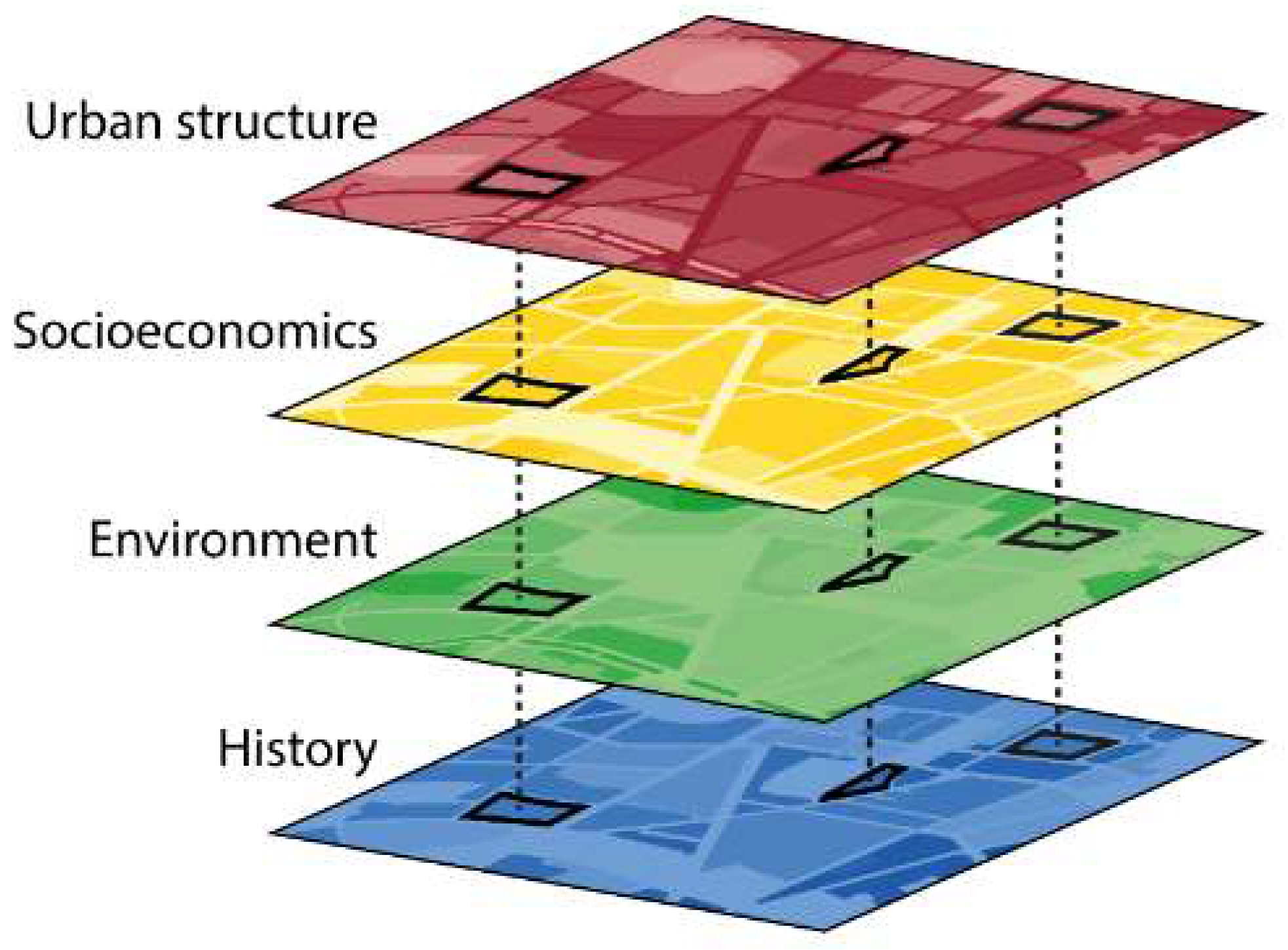
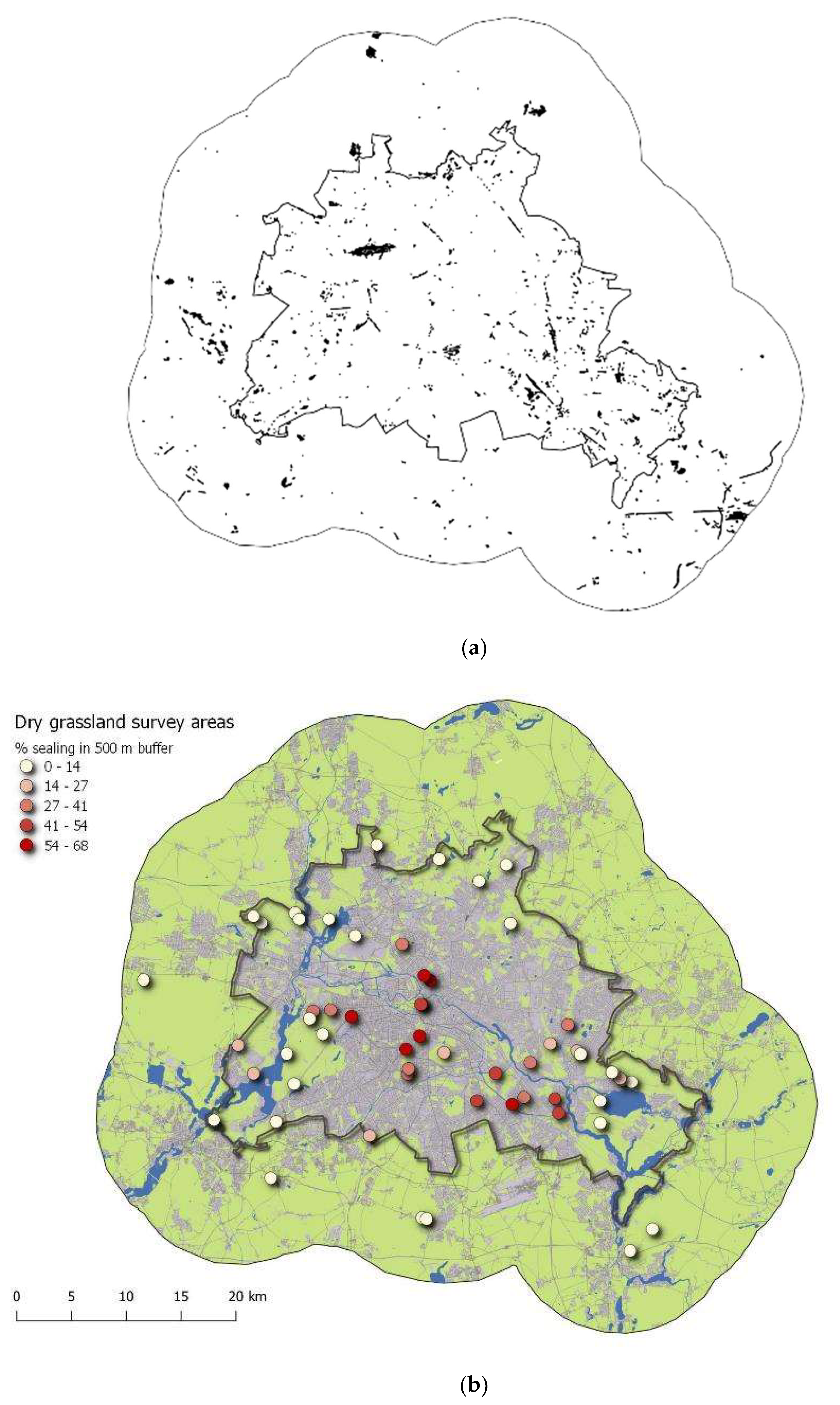
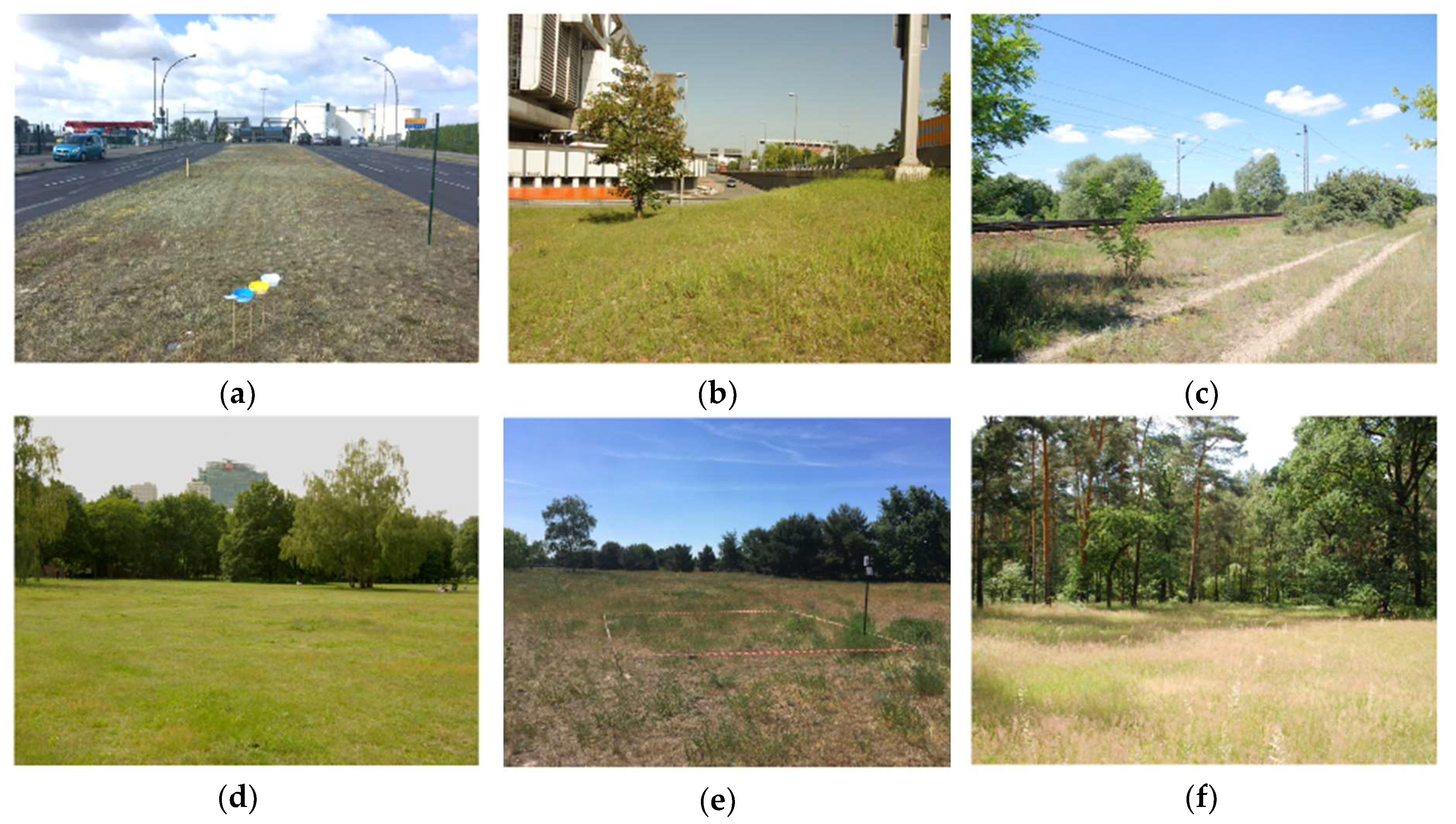
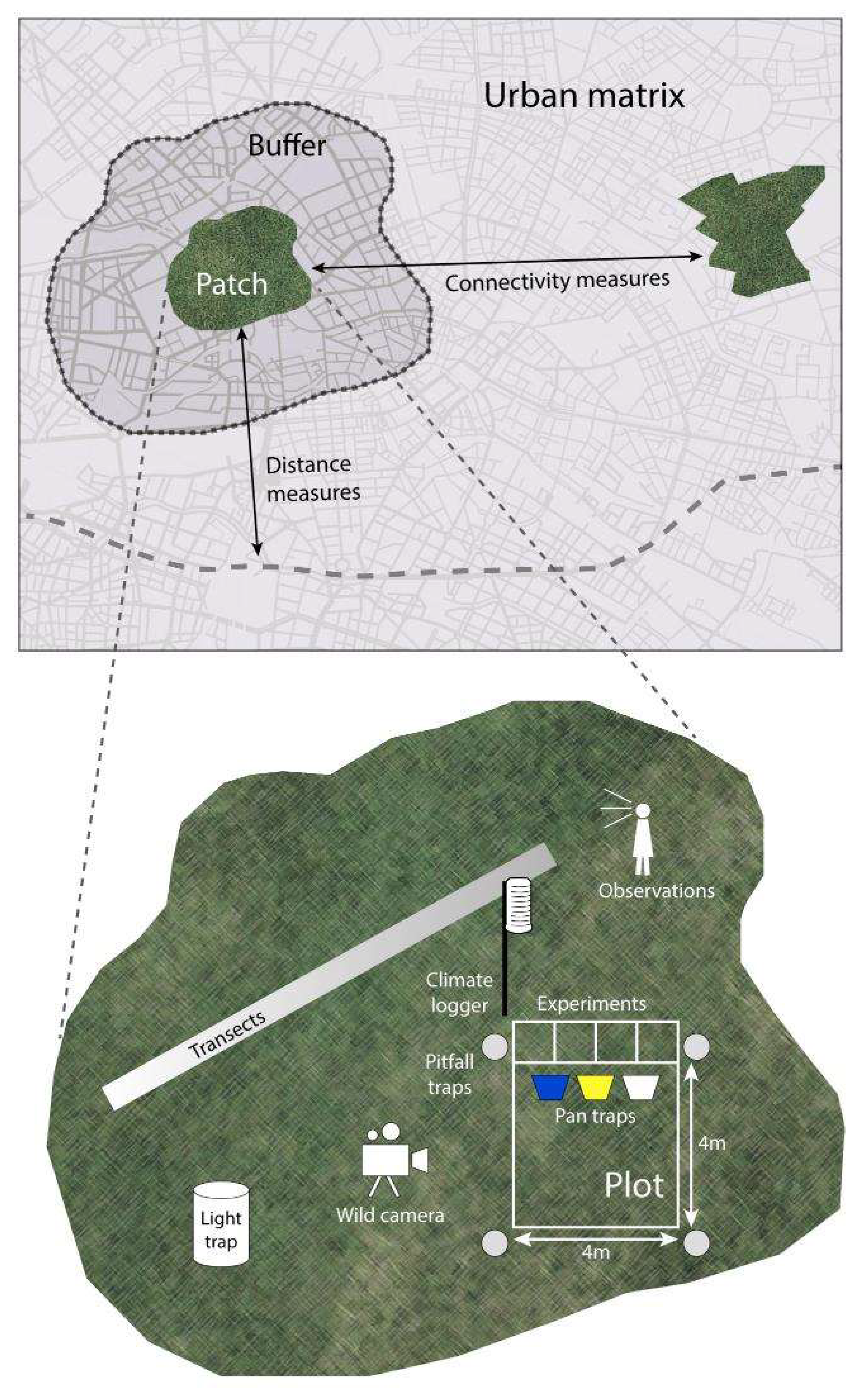
Table 1.
Taxa representing different functional or trophic groups that were recorded in the survey areas at different spatial scales (square = plot, line = transect, irregular shape = patch), with information about the presence (✔) of Red Lists (including total species lists) [123] and citywide distribution data at the city scale.
| Taxon | Spatial Scale in Survey Areas | Red Lists/Checklists at City Scale | Citywide Distribution Data | |
|---|---|---|---|---|
 | Plants (Plantae) |  | ✔ | ✔ |
 | Wild bees (Anthophila) | | ✔ | |
 | Hoverflies (Syrphidae) | | ✔ | |
 | Butterflies (Lepidoptera) |  | ✔ | |
 | Moths (Lepidoptera) | | ||
 | Grasshoppers (Orthoptera) | | ✔ | ✔ |
 | Ground beetles (Carabidae) | | ✔ | |
 | Rove beetles (Staphylinidae) | | ✔ | |
 | Woodlice (Isopoda) | | ||
 | Myriapods (Myriapoda) | | ||
 | Spiders (Araneae) | | ✔ | |
 | Harvestmen (Opiliones) | | ✔ | |
 | Sand lizard (Lacerta agilis) | | ✔ | |
 | Bats (Chiroptera) |  | ✔ | |
Table 2.
Environmental variables measured for the dry grassland study areas of the CityScapeLab Berlin, with unit, range or categories (depending on the type of variable), the spatial scale the variable refers to (plot, patch, buffer, distance), the year of measurement, the measuring method, equipment and software as well as data source and/or references. Note that “buffer” in “spatial scale” always refers to a buffer around the dry grassland patch, not the plot, and is calculated as a 100, 500, 1000, and sometimes 5000 m buffer.
| Variable | Unit/Range/Categories | Spatial Scale | Year | Method/Equipment/Software | Data Source/Reference |
|---|---|---|---|---|---|
| 1. Abiotic/Physical | |||||
| a. Microclimate | |||||
| Air temperature zone longtime medium 1961-1990 | °C | patch | 2016 | Software: QGIS Version 2.18.0 [118] | Berlin Environmental Atlas/Long-term Mean Air Temperatures 1961–1990 [129] |
| Urban climatic zone changes in temperature, air humidity, and wind regime compared to open land conditions | 0 = no; 1 = very low; 2 = low; 3 = medium; 4 = high changes | patch | 2016 | Software: QGIS Version 2.18.0 [118] | Berlin Environmental Atlas/Urban Climate Zones [130] |
| Air temperature values measured at 2 m height | ° C | plot | 2017 | Data logger: EasyLog EL-USB-2+, Lascar Electronics | |
| Relative air humidity measured at 2 m height | % | plot | 2017 | ||
| Dew point measured at 2 m height | ° C | plot | 2017 | ||
| Sky view factor share of open sky | 0–1 | plot | 2017 | Analysis of fisheye photos; Camera: Canon EOS 700D; Fisheye lens: SIGMA 4.5mm F2.8 EX DC HSM Circular Fisheye; Software: SOLWEIG1D Version 2015a [131] | Holmer et al. 2001 [124] |
| b. Light | |||||
| Skyglow value at a maximum cloudiness of 12.5 % | µcd/m² | plot | 2017 | Sky quality meter: Sky Quality Meter—L, Unihedron, Ontario, Canada | |
| Maximum illuminance at a maximum cloudiness of 12.5 % | lux | plot | 2017 | Lux meter: LX-1108, VOLTCRAFT, Hirschau, Germany | |
| Mean skyglow based on satellite data | µcd/m² | buffer | 2017 | Software: QGIS Version 2.14 [118] | Falchi et al. 2016 [132] |
| Mean light pollution based on aerial high resolution (1 m²) mosaic image | 0–… | buffer | 2017 | Software: QGIS Version 2.14 [118] | Kuechly et al. 2012 [133] |
| c. Soil chemistry | |||||
| pH value | 0–14 | plot | 2017 | Analysis of soil samples; Inductively coupled plasma optical emission spectrometry (ICP-OES): iCAP 6000 ICP Spectrometer, Thermo Fisher Scientific, Dreieich, Germany | Blume et al. 2011 [134] |
| Organic carbon (C) content | g/kg | plot | 2017 | ||
| Nitrogen (N) content | g/kg | plot | 2017 | ||
| Sulfur (S) content | g/kg | plot | 2017 | ||
| Phosphorus (P) content | mg/kg | plot | 2017 | ||
| Potassium (K) content | mg/kg | plot | 2017 | ||
| Copper (Cu) content | mg/kg | plot | 2017 | ||
| Zinc (Zn) content | mg/kg | plot | 2017 | ||
| Cadmium (Cd) content | mg/kg | plot | 2017 | ||
| Lead (Pb) content | mg/kg | plot | 2017 | ||
| Nickel (Ni) content | mg/kg | plot | 2017 | ||
| Gravimetric water content | % | plot | 2017 | ||
| Electrical conductivity in suspension | mS/m | plot | 2017 | ||
| Cation exchange capacity | µmolc/g | plot | 2017 | ||
| Carbon-to-nitrogen (C/N) ratio | % | plot | 2017 | ||
| Carbon-to-sulfur (C/S) ratio | % | plot | 2017 | ||
| 2. Spatial | |||||
| a. Continuity/Connectivity | |||||
| Historical continuity as grassland biotope | O = old (established before 1940); N = new (established after 1940) | patch | 2016 | Intersection of current dry grassland biotopes with historical grassland biotopes (from digitized and georeferenced historical land-use maps); Software: QGIS Version 2.18.0 [118] | Historical land-use maps: Preußische Uraufnahme (1831–71) [127], Preußische Neuaufnahme (1927–40) [128]; Berlin Environmental Atlas/Biotope Types [119], Biotope mapping Brandenburg [120] |
| Patch size of dry grassland | m² | patch | 2017 | Software: QGIS Version 2.18.0 [118] | Berlin Environmental Atlas/Biotope Types [119], Biotope mapping Brandenburg [120] |
| Share of dry grassland in the surrounding | 0–1 | buffer | 2016 | Software: QGIS Version 2.18.0 [118] | Berlin Environmental Atlas/Biotope Types [119], Biotope mapping Brandenburg [120] |
| Hanski’s connectivity index (HCI) based on pairwise distances (d) between plot (i) and dry grassland patches (j) and area (A) of the patches | 0–… | distance | 2020 | HCI = ∑j≠i exp(−α dij) Aj; Software: ArcGIS 10.3.1 for Desktop [135]; Tool: Generate Near Table (Analysis) | Berlin Environmental Atlas/Biotope Types [119], Biotope mapping Brandenburg [120]; Hanski 1994 [125] |
| b. Urbanity | |||||
| Sealed surface | % | buffer | 2017 | Software: QGIS Version 2.18.0 [118]; Tool: Zonal statistics | Berlin Environmental Atlas/Actual Use of Built-up Areas, Inventory of Green and Open Spaces 2010 [121] |
| Population size | number of inhabitants | buffer | 2017 | Software: QGIS Version 2.18.0 [118] | Berlin Environmental Atlas/Population Density 2015 [136] |
| Population density | inhabitants/ ha | buffer | 2017 | Software: QGIS Version 2.18.0 [118]; Tool: Zonal statistics | Berlin Environmental Atlas/Population Density 2015 [136] |
| Floor space index (FSI) | m² floor area/ m² lot area | buffer | 2017 | Software: QGIS Version 2.18.0 [118]; Tool: Zonal statistics | Berlin Environmental Atlas/Urban Structural Density [137] |
| Urban land cover (ULC) Built-up areas and traffic areas (biotope type 12 according to the Berlin classification of biotope types) | % | buffer | 2018 | Software: QGIS Version 2.18.0 [118] | Berlin Environmental Atlas/Biotope Types [119], Biotope mapping Brandenburg [120]; Hahs & McDonnell 2006 [70] |
| People per unit Urban Land Cover (PULC) Ratio of people divided by the proportion of urban land cover | inhabitants/ ULC | buffer | 2018 | PULC = Population/(ULC + 0.5); Software: QGIS Version 2.18.0 [118] | |
| Road density Total length of roads | km | buffer | 2017 | Software: QGIS Version 2.18.0 [118]; Tool: Sum line lengths | OpenStreetMap shapefile “osm_roads_line_2015_25833” [138] |
| Road distance Shortest distance from plot midpoint to nearest road | m | distance | 2017 | Software: QGIS Version 2.18.0 [118]; Tool: v.distance | |
| Railway density Total length of railways | km | buffer | 2017 | Software: QGIS Version 2.18.0 [118]; Tool: Sum line lengths | |
| Railway distance Shortest distance from plot midpoint to nearest railway | m | distance | 2017 | Software: QGIS Version 2.18.0 [118]; Tool: v.distance | |
| Distance to central business district Shortest distance from plot midpoint to Friedrichstraße station | km | distance | 2018 | Software: QGIS Version 2.18.0 [118]; Tool: v.distance | Hahs & McDonnell 2006 [70] |
| c. Landscape variables/Environment | |||||
| Number of biotope patches | number | buffer | 2018 | Software: QGIS Version 2.18.0 [118] | Berlin Environmental Atlas/Biotope Types [119], Biotope mapping Brandenburg [120]; Hahs & McDonnell 2006 [70] |
| Size of largest biotope patch | ha | buffer | 2018 | Software: QGIS Version 2.18.0 [118] | |
| Land cover richness Number of different biotope types (based on the highest level of the Berlin classification of biotope types) | 1–12 | buffer | 2018 | Software: QGIS Version 2.18.0 [118] | |
| Landscape shape index (LSI) Ratio of sum of edge length to total area for a landscape measured against a circle standard | 1–… | buffer | 2018 | LSI = Edge length/(2 * √(Pi * Area)); Software: QGIS Version 2.18.0 [118] | |
| Type of protected area | LCA = Landscape Conservation Area; NP = Nature Park; FFH = Flora Fauna Habitat Area; SPA = Special Protected Area according to Bird Conservation Directive; None | patch | 2016 | Software: QGIS Version 2.18.0 [118] | Berlin Environmental Atlas/Protected Areas by Nature Conservation Legislation (incl. Natura 2000) [139] |
| 3. Habitat structure | |||||
| Total vegetation cover | % | plot | 2017 | Estimation | |
| Cover of herbal layer | % | plot | 2017 | Estimation | |
| Cover of moss layer | % | plot | 2017 | Estimation | |
| Cover of litter layer | % | plot | 2017 | Estimation | |
| Height of herbal layer | cm | plot | 2017 | Estimation | |
| Degree of slope | ° | plot | 2017 | Estimation | |
| Aspect of sloped plots | 90° = East; 180° = South; 270° = West; 360° = North | plot | 2017 | Estimation | |
| Wild boars Digging traces | 0 = no; 1 = yes | plot | 2017 | Estimation | |
| Regular mowing at least once a year | 0 = no; 1 = yes | plot | 2017 | Estimation | |
| 4. Socioeconomic | |||||
| Unemployed people | % | buffer | 2018 | Software: QGIS Version 2.18.0 [118] | Geoportal Berlin/unemployment rate 2016 [140] |
| Inhabitants with migration background | % | buffer | 2018 | Software: QGIS Version 2.18.0 [118] | Geoportal Berlin/residents with migration background 2016 [141] |
| Mean living space per inhabitant | m² | buffer | 2018 | Software: QGIS Version 2.18.0 [118] | Geoportal Berlin/living space 2016 [142] |
| Occupancy of inhabitants People who have lived at the same address for at least five years | % | buffer | 2018 | Software: QGIS Version 2.18.0 [118] | Geoportal Berlin/residence over 5 years 2016 [143] |
© 2020 by the authors. Licensee MDPI, Basel, Switzerland. This article is an open access article distributed under the terms and conditions of the Creative Commons Attribution (CC BY) license (http://creativecommons.org/licenses/by/4.0/).
Share and Cite
MDPI and ACS Style
von der Lippe, M.; Buchholz, S.; Hiller, A.; Seitz, B.; Kowarik, I. CityScapeLab Berlin: A Research Platform for Untangling Urbanization Effects on Biodiversity. Sustainability 2020, 12, 2565. https://doi.org/10.3390/su12062565
AMA Style
von der Lippe M, Buchholz S, Hiller A, Seitz B, Kowarik I. CityScapeLab Berlin: A Research Platform for Untangling Urbanization Effects on Biodiversity. Sustainability. 2020; 12(6):2565. https://doi.org/10.3390/su12062565
Chicago/Turabian Stylevon der Lippe, Moritz, Sascha Buchholz, Anne Hiller, Birgit Seitz, and Ingo Kowarik. 2020. "CityScapeLab Berlin: A Research Platform for Untangling Urbanization Effects on Biodiversity" Sustainability 12, no. 6: 2565. https://doi.org/10.3390/su12062565
Note that from the first issue of 2016, this journal uses article numbers instead of page numbers. See further details here.