Control Strategy Optimization for Two-Lane Highway Lane-Closure Work Zones


1
Jiangsu Key Laboratory of Urban ITS, Southeast University, Nanjing 210096, China
2
Jiangsu Province Collaborative Innovation Center of Modern Urban Traffic Technologies, Southeast University, Nanjing 210096, China
3
Department of Civil & Environmental Engineering, University of Washington, Seattle, WA 98125, USA
*
Authors to whom correspondence should be addressed.
Sustainability 2019, 11(17), 4567; https://doi.org/10.3390/su11174567
Submission received: 13 July 2019
/
Revised: 10 August 2019
/
Accepted: 20 August 2019
/
Published: 22 August 2019
(This article belongs to the Section Sustainable Transportation)
Abstract
:Traffic control is very important for two-lane highway lane-closure work zone traffic management. Control of the open lane’s right of way is very similar to that of a two-phase signalized intersection. Thus, four control strategies including flagger control, pre-timed control proposed by Schonfeld, pre-timed control proposed by Webster, and actuated control are employed for possible use at work zones. Two primary methodologies, the mathematical delay model adopted from signalized intersections, and the simulation model calibrated with field data, are proposed. The simulation and mathematical results show that control strategies for two one-way road intersections could be used for two-lane highway lane-closure work zones. Flagger control after gap-out distance optimization prevails over all the other control strategies in terms of stopped delay, queue length, and throughput, under low or high volumes. Actuated control could be a good alternative for work zone areas due to its small queue length and large vehicle throughput under moderate volume conditions. Our findings may help to optimize the work-zone control strategy and improve operational efficiency at two-lane highway lane-closure work zones.
1. Introduction
A work zone is a section of roadway with construction, maintenance, or utility work activities [1]. These work activities are typically periodical and critical for a safe and efficient transportation system [2,3,4,5]. However, the decrease in speed and capacity caused by work zone activity often results in a bottleneck and may lead to queues for traffic approaching the work zone area.
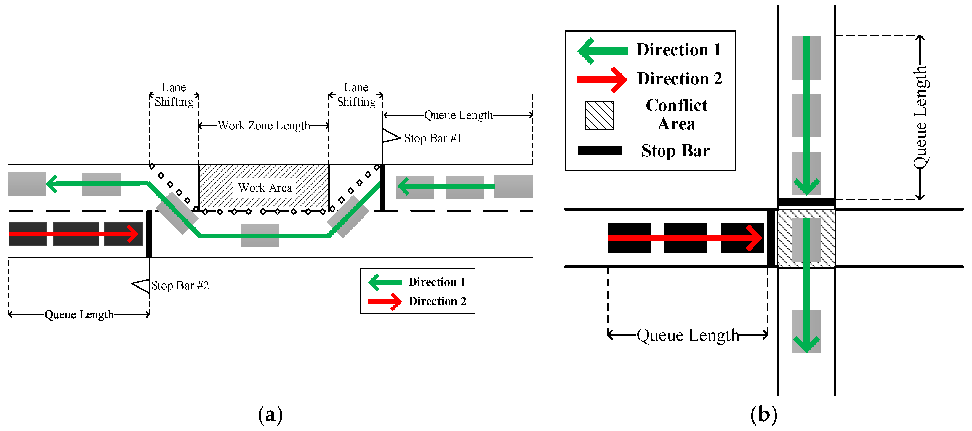
For a multilane highway (or freeway) work zone, the closure of one or two lanes will not necessarily lead to significant increases in user delay, especially when traffic volume is low to moderate. For two-lane highway work zones, a single lane closure has quite different implications. As shown in Figure 1a, when one lane is closed, vehicles in both directions have no choice but to use the single remaining lane. The queues and stopped delay are unavoidable under the circumstances.
Although two-lane highway lane-closure work zones are very common, previous research is still limited. To date, how to further improve control strategies for two-lane highway work zones to optimize traffic condition indicators, such as reducing delay and queue length, has not been well discussed. In addition, how two-lane work zone volume and speed limit affect delay, queue length, and throughput is not clearly stated as well. To address these, this study adopted four control strategies for two-lane highway work zones. A mathematical model for delay calculation and a simulation model for control strategies comparison and optimization were proposed. Further, other than delay, average and maximum queue lengths, and vehicle throughput were applied for different control strategies’ evaluation.
The remainder of the paper is structured as follows: First, a review of relevant literature is presented in Section 2. The configuration of a two-lane highway work zone is discussed in relation to that of a controlled intersection, and some widely used intersection control strategies are modified in Section 3. A theoretical model for the stopped delay calculation is made in Section 4. Section 5 describes the data collection and simulation model. Results for four different control strategies, with comparison and analysis, are shown in Section 6. Section 7 compares the performance of control strategies under different volume conditions and discusses the delays calculated by the mathematical model and by the simulation model. Conclusions and suggestions for two-lane highway lane-closure work zone control are given in Section 8.
2. Literature Review
A number of previous studies have focused on multilane work zone capacity and queue estimation [6,7,8,9,10], in order to reduce delay and promise total cost optimization [11,12,13,14]. However, multilane work zones are quite different from the scenarios in this paper. For two-lane highway work zones, right of way is allocated by flaggers (sometimes by signals) to traffic in each direction sequentially. To obtain a good operation performance of two-lane work zones, the control strategies as well as the delay caused by control should be well studied. One may see that the one-way control traffic is very similar to two-phase intersection control [15]. The intersection controls and the delay calculation models may have the potential to be applied for two-lane work zones after modification.
Several studies have focused on intersection control performance and delay estimation [16,17,18]. Broadly, there are two types of signal controls that have been used for intersections: pre-timed (or fixed-time) and actuated controls [19]. Generally, actuated control outperforms pre-timed control. However, pre-timed control is still widely used due to its advantages such as fewer loop detectors and simple implementation. The delay models are varied and can be classified into a deterministic queuing model, time-dependent stochastic delay model, shock wave delay model, and microscopic simulation delay model [20]. The time-dependent stochastic delay model, which can generate reasonable delay predictions, is widely used and recommended by the Highway Capacity Manual (HCM) [21].
Since control strategies are important for two-lane highway lane-closure work zones, studies have been done on this aspect. In 1987, Ullman and Levine [22] tested the performance of fixed-time control on two-lane, two-way highway work zones, and showed the fixed-time control would increase the delay time when compared with flagger control. Later, Schonfeld and Chien [23,24] proposed two mathematical models in 1999 and 2002 to optimize control strategies for two-lane highway work zones. The study illustrated that pre-timed control after optimization could minimize the total cost of traffic systems. Finley et al. [25] analyzed delay and performance under flagger control and pre-timed control. Based on the combination of field studies and simulation results, flagger control with assistance devices was more suitable for short-term stationary work zone operations, while pre-timed signal control was recommended for higher volume roadways. Zhu [15] proposed an optimal pre-timed signal control and dynamic flagger control. The results showed that dynamic control could be able to achieve a lower delay.
As for two-lane highway work zone delay and queue length analysis, mathematical models have been developed [15,22,23,24,26]. Generally, in the mathematical models, the delay time is estimated based on traffic demand, control strategy and plan, work-zone length, and vehicle speed. Based on the deterministic queuing theory and stochastic mathematical method, Cassidy [27,28] developed two delay estimation models and assessed the validity of models using Monte Carlo and microscopic simulations. The results showed that the performance of the proposed mathematical delay model is very close to that of the Monte Carlo method in terms of delay estimation.
Except for mathematical models, simulation methods have also been adopted to obtain the delay, queue length, and other indicators under different traffic conditions. In most simulation-based studies, delay and queue length were frequently used as indicators, to improve the performance of two-lane highway lane-closure work zones [15,29]. Ng [30] tried to minimize the total work zone travel time and employed a traffic flow theory-based cell transmission model. Chen [31] took detours into account and adopted agency cost and user cost as indicators, to optimize two-lane highway work zones by simulation. Other indicators, such as throughput, were seldom applied.
In addition, some agencies have developed their own models or software packages to address the challenges of work zone traffic control. QUEWZ and FRESIM are the most widely used macroscopic simulation tools. Both QUEWZ and FRESIM could overestimate the vehicle speeds under queuing conditions [32]. Furthermore, QuickZone [33], released by the Federal Highway Administration (FHWA) in 2005, can be used to estimate the work zone congestion impacts and recommend lane-closure schedules. However, the module for flagging operations in the software is inadequate for two-lane highways. In 2008, the Florida Department of Transportation developed an overall analysis procedure as well as a software tool (FlagSim) for two-lane highway work zones [34]. The procedure consists of a speed model, a saturation flow rate model, a capacity model, and queue delay and length models, as well as models for flagging control, vehicle distribution, and arrivals.
Based on the review of related literature on two-lane highway lane-closure work zone studies and models, some limits can be observed. Although attempts were made to find better control strategies, some advanced control methods, such as actuated intersection control, have not been applied for a two-lane highway work zone yet. Further, the performance of delay, queue length, and cost were evaluated under different volumes, speed limits, and work zone lengths. However, the relationship between them is not clear. This study adopts and compares some widely accepted and applied intersection control strategies for two-lane highway lane-closure work zones. Further, how traffic volume and speed limit affect delay, queue, and throughput is analyzed and discussed as well.
3. Problem Statement
Figure 1a illustrates a typical controlled work zone on a two-lane highway, and Figure 1b shows a two-phase intersection. In Figure 1a, there is only one open lane adjacent to the work zone area for traffic from both directions. Therefore, traffic from directions 1 and 2 must pass through the only remaining lane sequentially. When the vehicles from direction 1 have the right of way, vehicles from direction 2 must stop and wait behind the stop bar. Similarly, vehicles from direction 1 cannot pass through when the vehicles from direction 2 take up the lane. Thus, it can be seen in Figure 1a that traffic from directions 1 and 2 is sequentially allocated with right of way, which is analogous to a two-phase signal-controlled intersection as shown in Figure 1b.
Hence, if we rotate the road segment corresponding to direction 1 in Figure 1a by 90 degrees and consider the lane adjacent to the work zone area, in which the traffic from both two directions pass through, as an enlarged “conflict area”, the two-lane highway work zone can be considered nearly identical to the intersection shown in Figure 1b. Note, that usually, after rotation, the size of the “conflict area” for a work zone is relatively larger than that for an intersection. As a result, the clearance time must be long enough to make sure all the vehicles from both directions can get through this area.
Until now, flagger control has been the most commonly used control method for two-lane highway work zones. For intersections, on the other hand, a number of mature control methods have been developed, including pre-timed control, actuated control, and stop sign control. Considering the similarity between two-lane highway work zones and two-phase signal-controlled intersections, widely deployed intersection control methods and strategies show a great deal of promise for improving control in two-lane highway work zones. In this paper, two control strategies (i.e., Webster’s pre-timed control and actuated control) that have been frequently used in intersections are introduced for two-lane work zones. Additionally, flagger control and a work zone-optimal pre-timed control strategy proposed by Schonfeld [24] are employed for comparison. In all, a total of four control strategies are tested for two-lane highway work zones. Some detailed information about the control strategies is provided in the following section.
3.1. Control Strategy 1: Flagger Control
Flagger control is a manual or semi-automated control strategy and is often used for one-lane two-way road conditions. Flaggers hold or remotely operate a paddle with “Stop” on one side and “Slow” on the other side to indicate to vehicles to slow down, stop, and pass through. To provide coordination of the control, flaggers often communicate with other flaggers using handheld radios, with each standing at opposite ends of the work zone (See the left top in Figure 3).
Because right of way is allocated by flaggers manually, it is very hard to describe the control strategy in mathematical terms. In Reference [34], Washburn et al. proposed a flagging method (i.e., the distance gap-out method) that can be used to simulate and optimize flagger control strategies. The core idea of the distance gap-out flagging method is that when the distance between approaching vehicles on the current right of way exceeds a specified distance gap, the right of way is given to the opposite direction. This ends up being quite similar to reality: A flagger in charge of one direction will switch right of way to the opposite direction when the headway (or distance) between two vehicles is large enough to indicate that the queue has cleared. In this paper, the distance gap-out method was adopted as control strategy 1. More detailed information can be found in Reference [34].
3.2. Control Strategy 2: Pre-Timed Control (Proposed by Schonfeld)
In 1999, Schonfeld and Chien [23] proposed a queuing theory-based mathematical model to optimize traffic control on two-lane highway work zones and obtained a group of formulas. In their study, they assumed that: (1) The speed and travel time in the zone are the same for both directions, and (2) the departure rate for both directions is the same. In this paper, we employed the optimal fixed time control plan from their paper but relaxed the above assumptions. The resulting formulas for the optimal green time in each direction are as follows:
where Gi (i = 1, 2) denotes the optimal green time for direction i; Qi (i = 1, 2) denotes the number of arrival vehicles per hour (i.e., hourly flow rate) for direction i; Pi (i = 1, 2) denotes the discharge rate for direction i; and ri (i = 1, 2) is the average travel time in the remaining lane adjacent to the work zone for direction i. Note that ri is also the clearance (i.e., all red) time for direction i.
The discharge rate Pi can be obtained from 3600 s (one hour) divided by the Hi (average headway for vehicles running at the remaining lane adjacent to work zone area) as follows:
The average travel time, ri (i = 1, 2) can be calculated from the work zone length divided by the average travel speed at the only open lane adjacent to the work zone area. Note that even though the average speeds for both directions at the open lane are the same, the clearance time of the lane-closure direction is larger due to the extra lane shifting time from the closed lane to the adjacent lane, and then from the adjacent lane back.
If the yellow time is neglected (or included in the green time), the cycle length C can be formulated as
The detailed derivation of Equations (1)–(4) and further discussion about the optimal control plan are illustrated in the next section.
3.3. Control Strategy 3: Pre-Timed Control (Proposed by Webster)
In 1958, Webster [35] proposed an optimal minimum delay cycle length model for signal intersections based on a series of experiments, as follows:
where Cop denotes optimal cycle length; Y is the sum of critical phase flow ratios; and Lop is the total lost time within the cycle. Because there is no typical start-up lost time for two-lane work zones, the start-up lost time for intersections in HCM, 2 s, was adopted. The total lost time can be obtained then by:
By substituting the total lost time Lop into Cop and expanding Y, the optimal cycle length of strategy 3 used in the paper is expressed as follows:
where Si represents the saturation flow rate and can be calculated by Washburn’s model [34]. With Equation (7), the optimal minimum delay cycle length for the two-lane highway work zone can be obtained. Then, the green time for each direction can be calculated following Webster’s original model in Reference [35].
3.4. Control Strategy 4: Actuated Control
Control strategy 4 is actuated control. In actuated control, the cycle length, phase splits, and even phase sequence can be dynamically changed in response to the real-time vehicle actuations registered at detectors or at other traffic sensors. Thus, a major advantage of actuated signal control is its flexibility in adjusting cycle length and phase sequence to accommodate traffic fluctuations. This control strategy can be divided into semi-actuated and fully actuated control, according to the number of traffic movements that are detected. Fully actuated control uses detectors on all legs of a crossroad. This type of control is applicable to crossroads that contain fluctuations in traffic flow, while semi-actuated control is implemented at the crossroad between major and minor streets with detectors placed only on the minor street leg. In this paper, a fully actuated control with only one ring and no barrier was used, which strictly follows the rules and instructions contained in the Manual on Uniform Traffic Control Devices (MUTCD) and Traffic Detector Handbook [36,37].
4. Mathematical Model Development
Because two-lane highway lane-closure work zone control is a kind of one-way traffic control, the four control strategies can cause varying levels of queuing and stopped delay. This section illustrates the procedures used in developing a mathematical model based on Schonfeld and Chien’s study [23] that describes two-lane highway work-zone delay calculation.
From the above control strategies 2, 3, and 4, the maximum queuing time for directions 1 and 2 are (G2 + r1 + r2) and (G1 + r1 + r2), respectively, while the discharging times (namely, green time) for directions 1 and 2 are G1 and G2. The maximum queuing length is the hourly flow rate multiplied by the maximum queuing time. Assuming the queues are discharged within one cycle, G1 and G2 can be formulated as
Solving Equations (8) and (9), G1 and G2 can be obtained, as shown in Equations (1) and (2).
The deterministic stopped delay time per cycle for directions 1 and 2 (Y1,1 and Y1,2, respectively), and deterministic stopped delay time in mean vehicle delay (d1,1 and d1,2) can be calculated by Equations (10) and (11):
Thus, the deterministic stopped delay in mean vehicle delay can be derived as follows:
where L is the length of the work zone, and Vi is the average travel time in the remaining lane adjacent to the work zone for direction i.
Although deterministic delay models are simple, real traffic flows may not be uniform. More general delay models should account for the stochastic features in vehicle arrival patterns. Further, the delay caused by oversaturated flow should be taken into consideration. For stochastic and oversaturated traffic flows, the incremental delay is adopted, based on the HCM 2010 model [21]:
where T denotes the analysis time, Xi denotes the volume-to-capacity ratio, m is the vehicle arrival adjustment factor accounting for the randomness in vehicle arrival rates, k is controller setting adjustment factor, and I is upstream filtering/metering adjustment factor. In HCM 2010, k is 0.5 for pre-timed control, and I = 1.0 for isolated signals. These two values are also used in this study.
The average stopped delay in mean vehicle delay can be calculated using Equation (14).
5. Simulation Model Development
5.1. Field Data Description
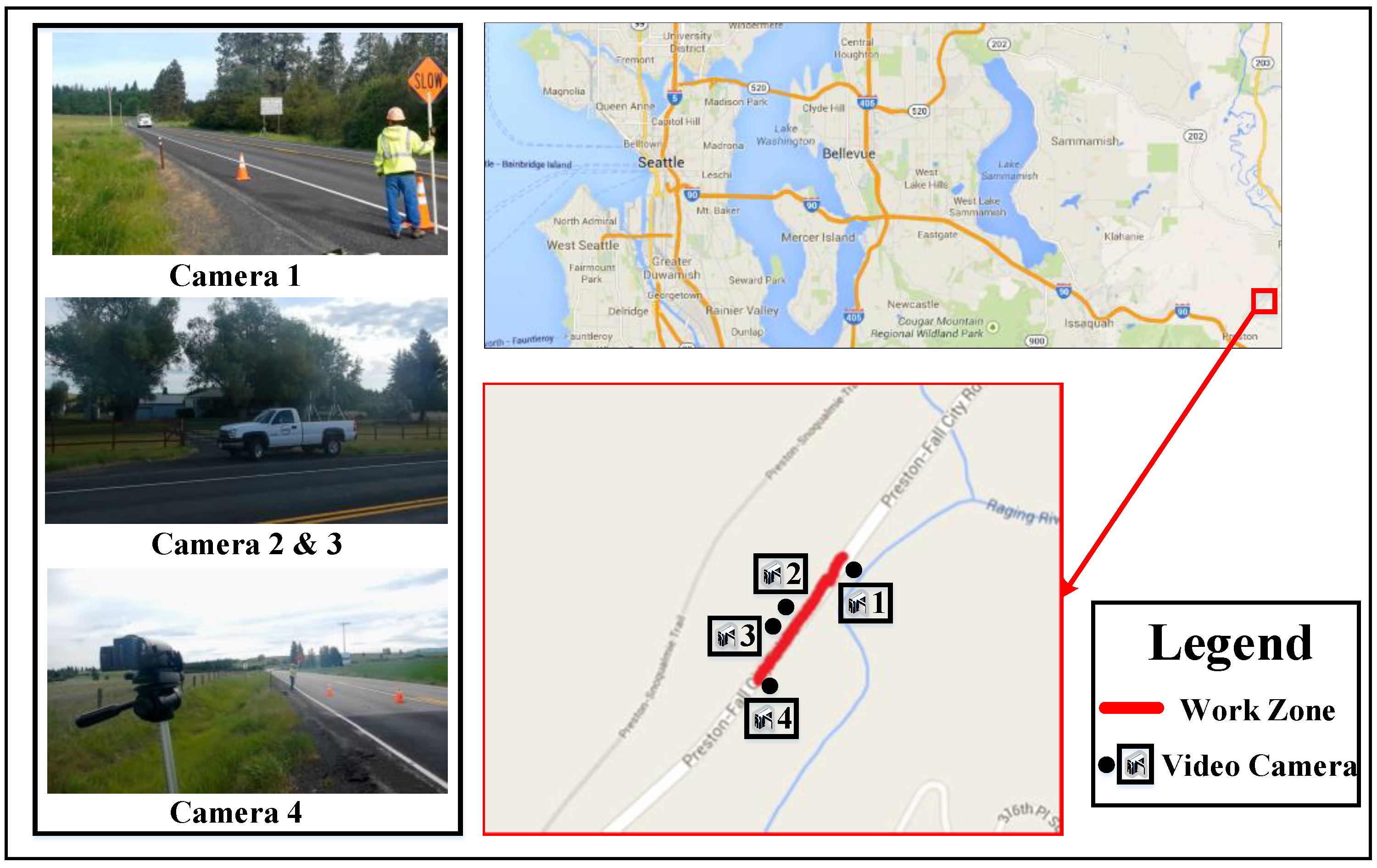
To develop and calibrate simulation models for comparing control strategies and investigating the relationship between average speed, hourly flow rate, and three traffic condition indicators, two-lane two-way work zone field data were collected from a 243.84-m-long work zone on Preston-Fall City Road SE, near the I-90 Corridor in Washington state, USA (Figure 2). Along the work zone area, no intersection and few access points exist. The data-collection work was part of the National Cooperative Highway Research Program (NCHRP) 3-107 project tasks [15].
Four video cameras were set up to collect traffic data, as shown in Figure 2. Cameras 1 and 2 captured northeastward, while the others were used to capture southwestward. All the cameras were placed high enough to make sure all the vehicles could be captured clearly. Data collection was conducted around 1 hour per day, on Monday, 29th July 2013, Wednesday, 14th August 2013, and Monday, 19th August 2013. The following information was collected and used in this paper: hourly flow rate, trucks percentage, headway, arrival time, and departure time for each vehicle as well as work zone travel time for each vehicle. Summary statistics of the collected data are illustrated in Table 1.
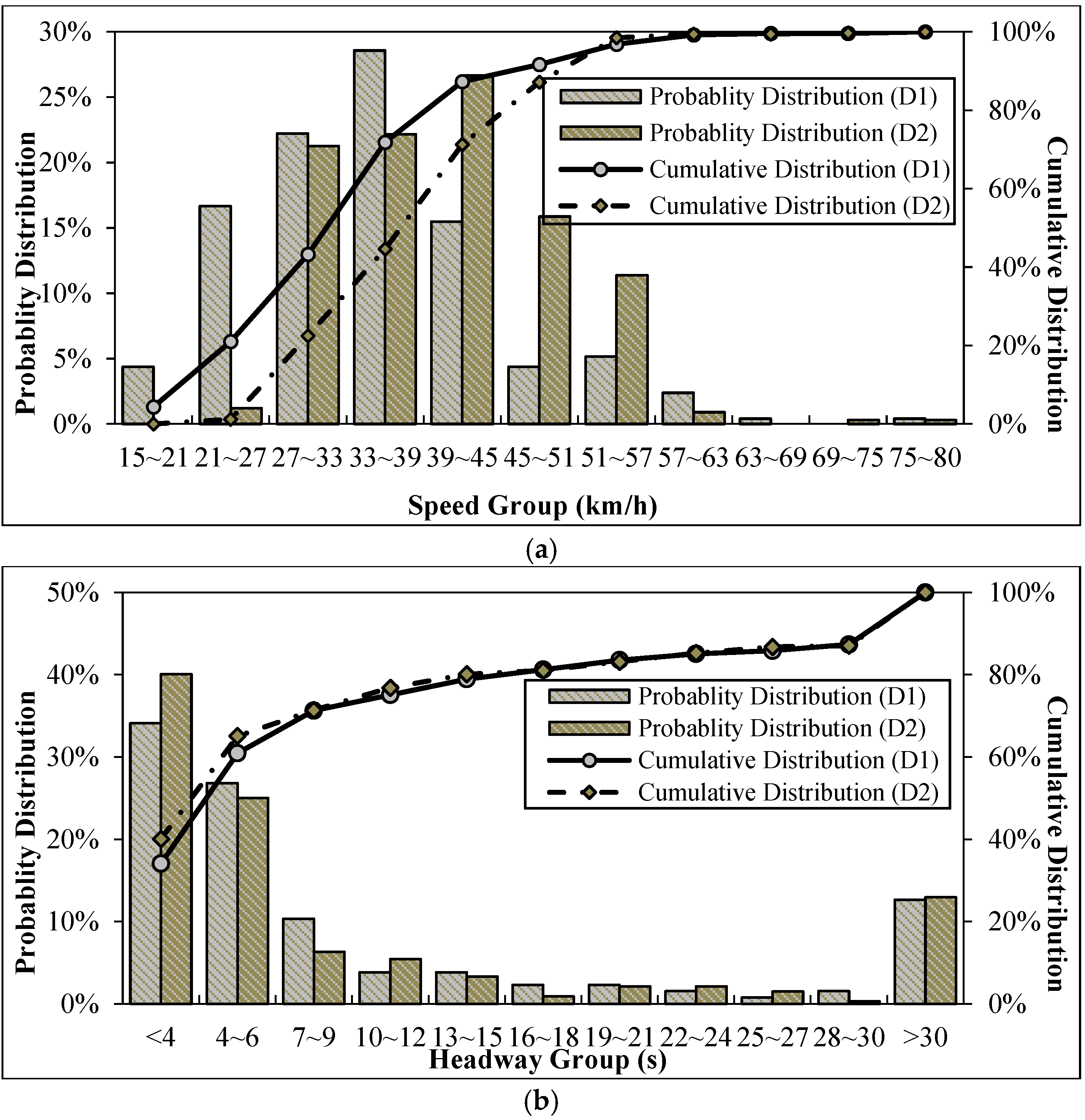
Figure 3 demonstrates some more detailed information about the field date on speed and headway distribution. For direction 1, the speed associated with the greatest frequency is 33–39 km/h, while the most frequent speed for direction 2 is higher (39–45 km/h). This makes sense because the vehicles from direction 1 have to slightly reduce their speed to make sure they can change back to the right lane after passing through the work zone. In addition to speed, the flow rate can also affect the performance of the work zone to some extent. Because the field data only covers approximately 1 h, there is limited variation in flow rate. Instead, headway, the reciprocal of flow rate, is used in this analysis. From Figure 4b, around 35% of the headways are less than 4 s, and more than half are under 7 s. There are also some differences in headway between two directions. On direction 2, the percentage of headways smaller than 4 s is greater than that for direction 1. The headways on direction 1 tend to be slightly higher and more spread out, with a greater percentage appearing in the majority of headway bins over 4 s. Comparing the average headway of direction 1 with direction 2, the headway in direction 1 is slightly larger, which indicates the flow rate of direction 1 is smaller than that for direction 2.
5.2. Simulation Model Development
This research employed VISSIM (Version 5.40), a widely used and proven microscopic traffic simulation software, to evaluate the performance of four control strategies on a two-lane highway work zone. This study has three types of simulation parameters (or models) that need to be determined. Type 1 is traffic simulation environment parameters, such as the layout of the work zone, speed, volume, and truck percentage. This kind of parameter can be calibrated directly using the field data. Type 2 is the gap-out distance, which can be used to fit the model to the observed flagger control strategy. Type 3 is the VISSIM built-in models, such as lane changing and travel behavior models. Type 2 and 3 parameters can be calibrated simultaneously.
To sufficiently populate the road with traffic, simulation time was set to 75 min, with the first 15 min being “seeding time”. Since the VISSIM is a stochastic model, some small differences in results are to be expected with different random seeds. To address this issue, each simulation was run five times with different random seeds. The reported simulation results, then, are the average over five runs.
Average stopped delay from field data and simulation were compared to validate the accuracy of the calibrated VISSIM model. Percentage error (PE) was used to measure the difference between observed and simulated delay. Defining as the simulated delay and as the measured delay, PE can be obtained following Equation (15):
Figure 4 shows the calibration results. The values of percentage error range from 0% to 33% for different gap-out distances. When the threshold value of gap-out distance for direction 1 is 85.3 m and for direction 2 is 91.4 m, the best goodness-of-fit is achieved with PE values of 0.1% and 0.4% for directions 1 and 2, respectively. In addition, the optimal flagger control strategy is found when the gap-out distance is 48.8 m. In other words, the flaggers shifted right of way to the opposite direction when the distance between two approaching vehicles exceeded 91.4 m. If this distance is reduced to 48.8 m, the control stopped delay would be minimized.
The driving behavior model was calibrated as well. Byungkyu [38] applied a genetic algorithm-based simulation model calibration and validation procedure for work zone networks and recommended parameter values for the Wiedemann 99 model. In this paper, the default values of the Wiedemann 99 model were compared with values from Byungkyu’s study. The results showed that the default values are more suitable when compared with Byungkyu’s recommended ones. In the final model, the default values of the Wiedemann 99 model were used, with the exception of CC0 (standstill distance), which was set to 1.06 m.
6. Result Analysis
6.1. Simulation Performance with Field Data
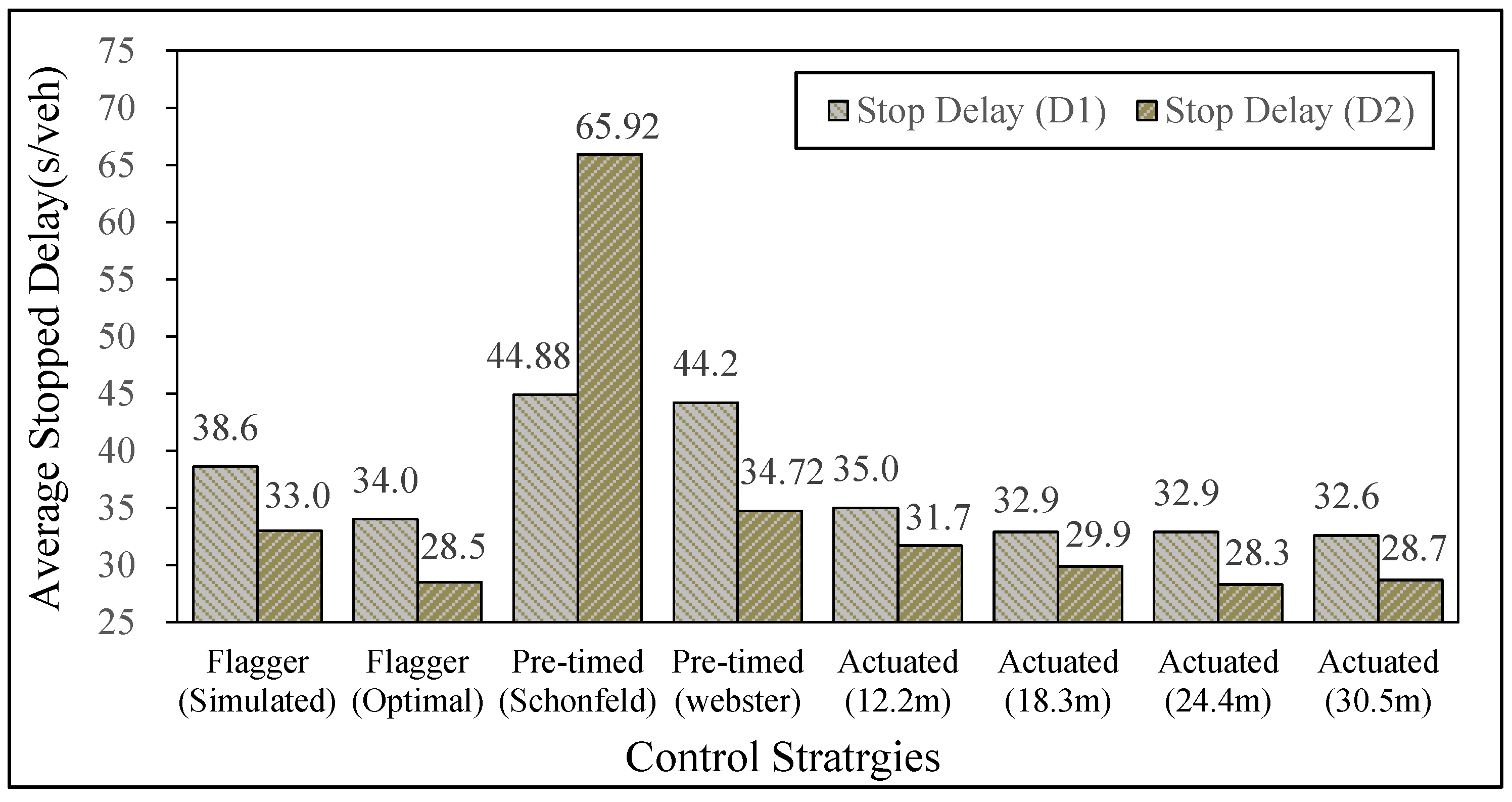
In this subsection, the four control strategies proposed in this paper are analyzed based on the simulation results. Figure 5 illustrates the average stopped delay for different control strategies. Because the distance between the loop detector and stop bar may also have an influence on stopped delay, four typical distances, 12.2 m, 18.3 m, 24.4 m, and 30.5 m, were tested. Additionally, for control strategy 1 (flagger control), three gap-out distances were employed: 85.3 m (direction 1) and 91.4 m (direction 2) gap-out distance were used for the simulated flagger control, while 48.8 m was used for the optimal flagger control.
As shown in Figure 5, the frequently-used intersection control strategies, both pre-timed and actuated, work very well for the two-lane highway work zone. The stopped delays for pre-timed control (Webster) in directions 1 and 2 are 44.2 s and 34.7 s, respectively, which are very close to those of flagger control (simulated). The performance of actuated control is even better. The stopped delays are 35.0 s, 32.9 s, 32.9 s, and 32.6 s for actuated control in direction 1 (D1), and 31.7 s, 29.9 s, 28.3 s, and 28.7 s for actuated control in direction 2 (D2) when the distance between the loop detector and stop bar is set to 12.2 m, 18.3 m, 24.4 m, and 30.5 m, respectively. Compared with optimal flagger control, with a stopped delay of 34.0 s (D1) and 28.5 s (D2), actuated control shows a tenuous advantage when the distance between the loop detector and stop bar is larger than 18.3 m.
For the two work zone control strategies, the performance depends on several factors. As the most widely used strategy, the performance of flagger control is acceptable, especially after optimization. The stopped delays of flagger control before and after optimization are, respectively, 38.6 s and 34 s for direction 1, and 33.0 s and 28.5 s for direction 2. This gives a delay reduction of approximately 15% resulting from optimization. Pre-timed control (Schonfeld), on the other hand, performs worst with the largest delay of 44.88 s for D1 and 65.9 s for D2. Schonfeld’s work zone optimization models might not be ready for implementation in terms of delay.
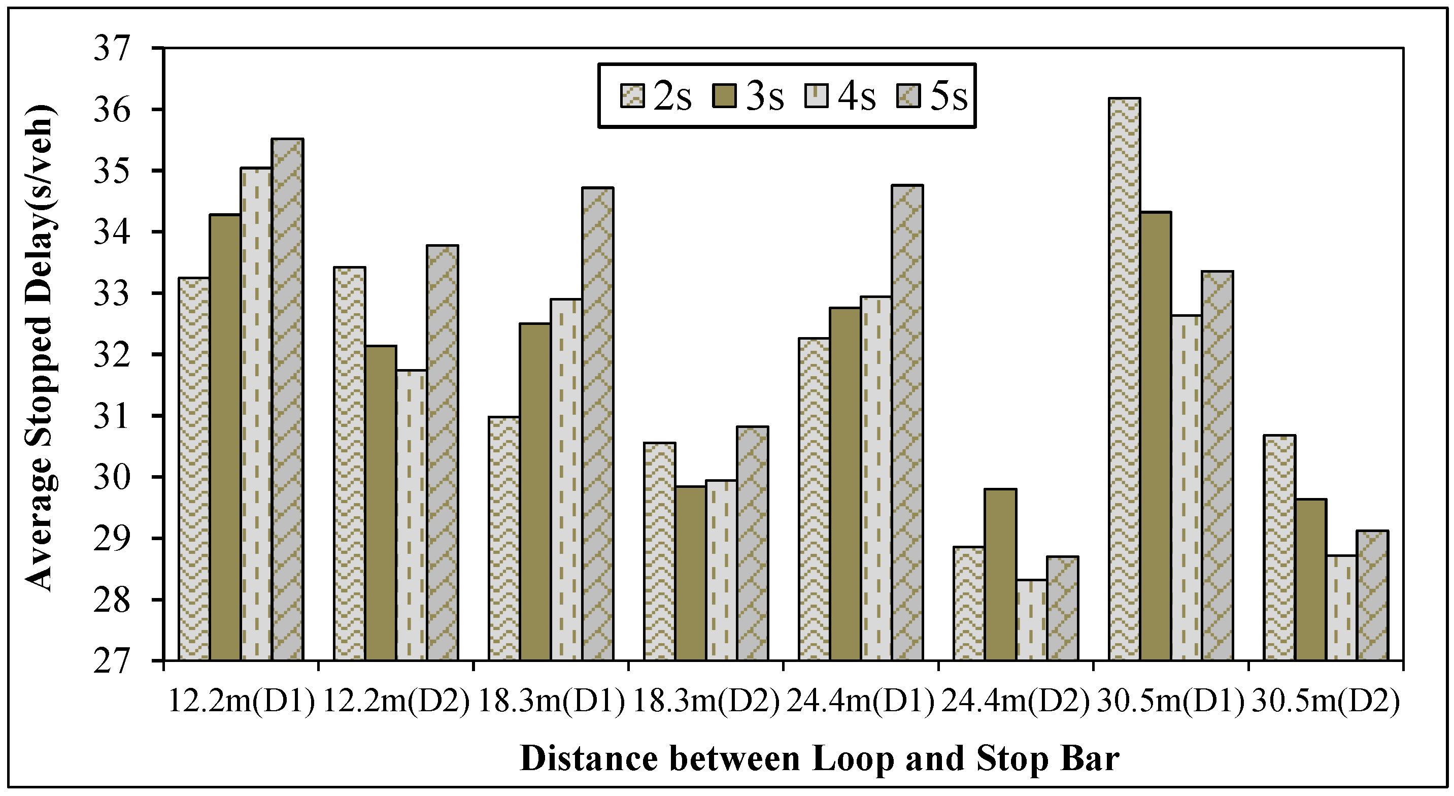
Because the green extension time may also affect the performance of actuated control, four green extension times were tested (Figure 6). The green extension time was calculated such that a vehicle can travel from the detector to the stop bar. For direction 2, the stopped delay would decrease at the lower values for green extension time. When the green extension time is set to 4 s, the stopped delay is minimum. Above 4 s, stopped delay of direction 2 begins to increase. For direction 1, the situation is a bit more complicated. When the green extension time is increased from 2 s to 5 s, the stopped delay of direction 1 grows if the distance between the loop detector and stop bar is smaller than 24.4 m. If the distance is 30.5 m, the delay trend for both directions is the same. Although change trends vary for directions, if using the total stopped delay as an evaluation criterion, a 4-s green extension time is optimal for actuated control as it produces the lowest total stopped delay. Thus, in this paper, the green extension time adopted for actuated control was set as 4 s.
6.2. Impact of Control Strategies on Stopped Delay
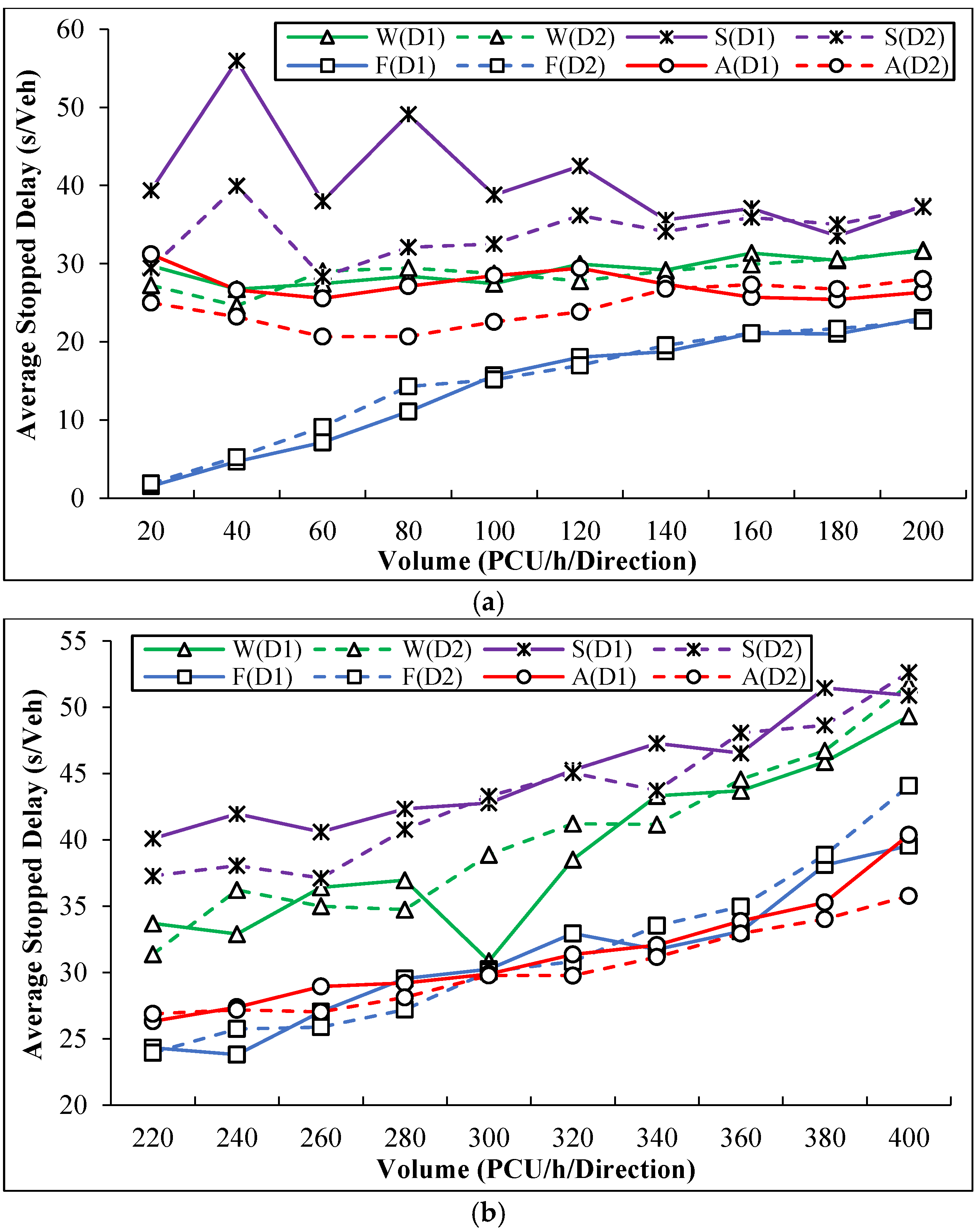
Although flagger control and actuated control perform better than the others with the field data, if the two parameters (i.e., volume and speed) change, the relative performance of these strategies may vary as well. Figure 7 illustrates the performance of the four control strategies under low volume (20–200 PCU/h/direction), moderate volume (220–400 PCU/h/direction), and high volume (420–580 PCU/h/direction) respectively, with respect to stopped delay. In the figure, W means pre-timed control (Webster), S denotes pre-timed control (Schonfeld), F denotes the optimal flagger control, while A is actuated control (24.4 m, see Figure 6). The volume increases from 20 to 580, with an interval of 20. The maximum volume for both directions is set to 580 PCU/h, owing to the fact that (1) the volume-to-capacity ratio is relatively large, i.e., around 0.9 (for actuated control, the volume-to-capacity ratio has exceeded 1) when the volume is 580 PCU/h/direction; and (2) the work zone area is totally congested, so both the stopped delay and queue length are far from the normal ranges if the volume is over 580 PCU/h/direction.
When the volume is low (Figure 7a), the performances of the four control strategies are varied. The optimal flagger control outperforms the other three with respect to the stopped delay, especially when the volume is lower than 100 PCU/h/direction. The biggest stopped delay of the optimal flagger control is comparable to the smallest stopped delay of the others. The stopped delay caused by pre-timed control (Webster) is a little bit larger but close to that caused by actuated control. Pre-timed control (Schonfeld) performs the worst with the biggest stopped delay. Note that with the volume increase, the stopped delay of the optimal flagger control, actuated control, and pre-timed control (Webster) will increase, while the stopped delay of pre-timed control (Schonfeld) will decrease first and then go up. Because Schonfeld assumed that vehicles could arrive at the work zone area uniformly, when the volume is low, the cycle length, as well as the green time of the pre-timed control (Schonfeld), are shorter and unnecessary for all vehicles to pass through the work zone without stops. As a consequence, the stopped delay is abnormally larger when the volume is low.
With the volume increase from 220 PCU/h/direction to 400 PCU/h/direction (Figure 7b), the growth trends of the stopped delay caused by the four control strategies are comparable. Flagger control and actuated control, which perform very close with the lower stopped delay, outperform the other two control strategies. Pre-timed control (Schonfeld) remains the worst with respect to the stopped delay.
When the volume is over 420 PCU/h/direction (Figure 7c), the increase of the stopped delay is faster. The optimal flagger control remains the best control strategy with the lowest stopped delay. The performance of actuated control is nice if the volume is lower than 500 PCU/h/direction. However, when the volume increases from 500 PCU/h/direction, the increase of stopped delay of actuated control starts to speed up, thus making actuated control a little worse than flagger control. The two pre-timed controls are the worst strategies with the largest stopped delay, especially the one proposed by Schonfeld, which suddenly starts to jump at 540 PCU/h/direction.
In general, the optimal flagger control outperforms the other control strategies under any volume conditions. Conversely, pre-timed control (Schonfeld) is the worst with respect to the stopped delay. When the volume is moderate, the actuated control strategy is as perfect as the optimal flagger control. Especially when the volume is between 300P CU/h/direction and 460 PCU/h/direction, the stopped delay caused by actuated control is even smaller.
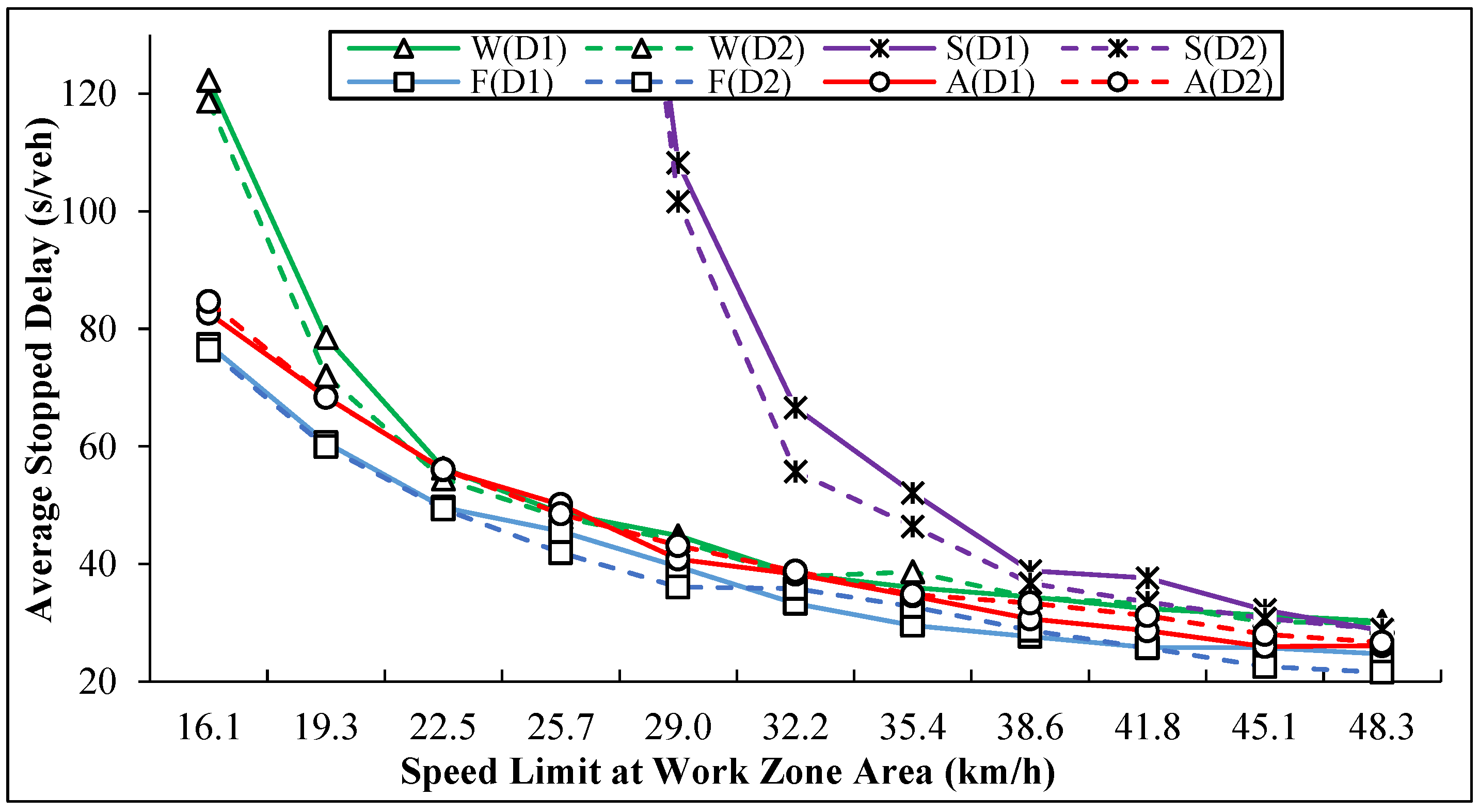
The value of the speed limit at the work zone area can affect the stopped delay as well (Figure 8). The volume in this figure is set constant to 250 PCU/h/direction to minimize the influence of volume on control. From the figure, it is clear that with an increased speed limit, the stopped delay decreases for all four control strategies. Actuated control outperforms both pre-timed controls but is still a little worse than the optimal flagger control whenever the speed is low or high. This indicates that according to the performance, the sequence of the four strategies remains unchanged if the volume is constant. In addition, the influence of speed limit change on pre-timed control (Schonfeld) is greater than on the others. When the speed limit is set to 16.1 km/h, the stopped delay of pre-timed control (Schonfeld) is more than 1400 s, which is 12 times the stopped delay of pre-timed control (Webster) and 17.5 times the stopped delay of the flagger control and actuated control. Considering that the impact of speed on delay is quite similar to the impact on other traffic condition indicators, in this paper, the speed limit will be constant, which equals to the field data collected.
6.3. Impact of Control Strategies on Queue Length
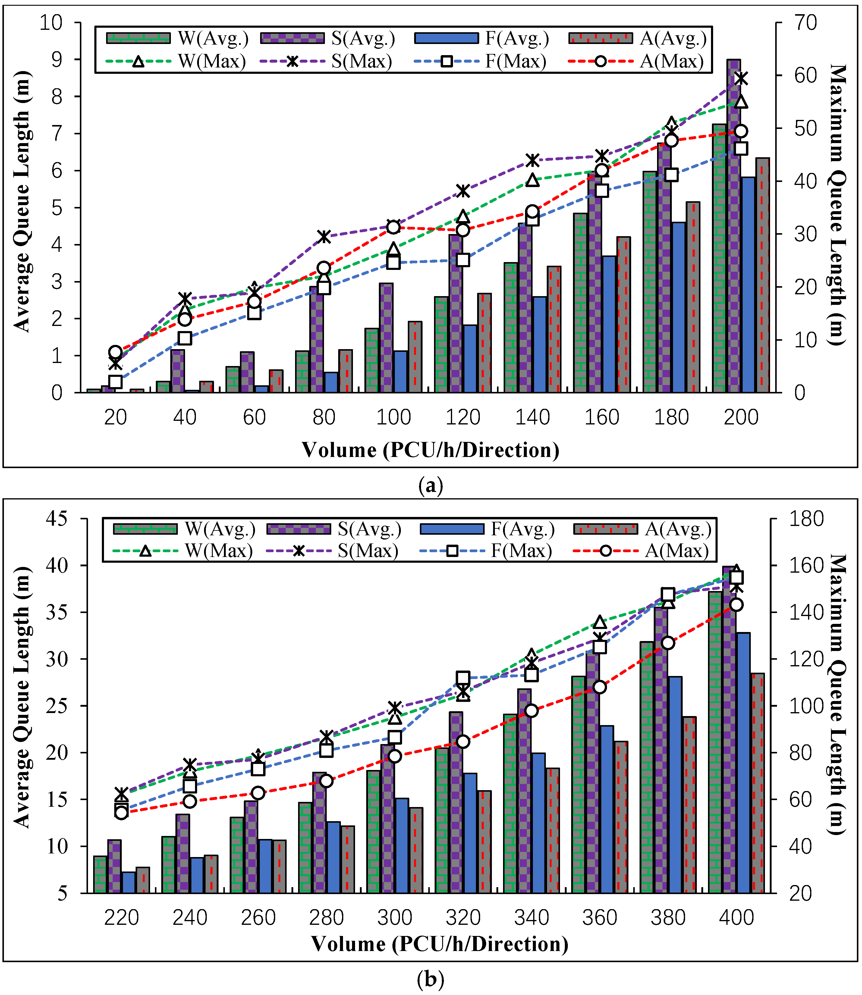
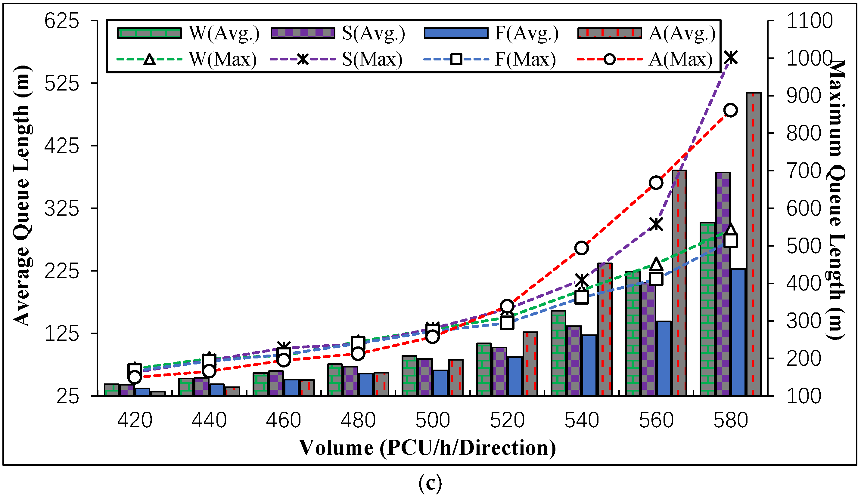
The queue lengths of the work zone area under the four different control strategies were also analyzed, as Figure 9 shows. The average and maximum queue lengths are both illustrated to make a more objective evaluation.
Under a low-volume condition (Figure 9a), the average queue length differences between four types of control strategies varied from 0 to 3 m. Compared with pre-timed control (Webster and Schonfeld), flagger control and actuated control show a tenuous advantage with respect to the average queue length. Under a moderate-volume condition (Figure 9b), actuated control gradually became superior to other strategies. More remarkably, the average queue length differences were over 10 m, which indicated a great influence. Under a high-volume condition (Figure 9c), flagger control overtook the others, especially when the volume was over 560 PCU/h (nearly congested).
Simulated results demonstrate that the optimal flagger control outperforms both pre-timed controls (Webster and Schonfeld) whenever the volume is low or high. Other than pre-timed control, actuated control shows a great superiority, especially under moderate volume. However, when the volume exceeds 500 PCU/h, the queue length of actuated control increases dramatically as the volume grows. Therefore, in terms of queue length, actuated control could be a good alternative in low- or moderate-volume conditions. However, when traffic is heavy, flag control has played an irreplaceable role in reducing queue length.
6.4. Impact of Control Strategies on Throughput
In addition to the stopped delay and queue length, the vehicle throughput with different vehicle inputs was simulated and collected as well, as shown in Figure 10. Because throughput will gradually increase as vehicle input goes up, it is hard to tell whether the change pattern of throughput is caused by input or other factors. To make it more straightforward, another indicator, the difference between vehicle input and throughput, was employed. The difference between vehicle input and throughput can be obtained simply by subtracting the throughput from the input. It is obvious that the smaller the difference is, the better the control strategy performs.
From Figure 10a, under a low-volume condition, actuated control overtakes the others. Especially when the volume ranges from 40 PCU/h/direction to 80 PCU/h/direction, the throughput is even a little bit more over the input. The optimal flagger control, compared with both pre-timed controls, shows a tenuous advantage in terms of throughput, except when the volume equals 200 PCU/h. Pre-timed control (Schonfeld) performs better than the other pre-timed control at most volume conditions.
Under a moderate-volume condition (Figure 10b), the difference between vehicle input and throughput shows something special compared to that under low volume. Actuated control, though, remains the best control strategy, being able to let up to seven more vehicles pass through the work zone area per hour when compared to the vehicle input. The optimal flagger control performs worse than the actuated control; however, it outperforms both pre-timed controls. Pre-timed control (Webster), which is the poorest control strategy with respect to throughput when the volume is low, outperforms pre-timed control (Schonfeld), especially when the volume is under 360 PCU/h.
Under a high-volume condition (Figure 10c), instead of actuated control, pre-timed control (Schonfeld) shows a great superiority, while the previous best strategy, actuated control, drops to being the last alternative. Note, that if the volume is over 480 PCU/h, the difference between the input and throughput caused by actuated control surges dramatically, which indicates that actuated control is not an option for high volume.
In summary, compared to the other strategies, actuated control can let more vehicles pass through the work zone area. However, when the volume is over 480 PCU/h, the throughput of actuated control drops sharply. The optimal flagger control, though, performs worse than actuated control but better than pre-timed control most times. Pre-timed control (Schonfeld) is treated as the best one only when the volume is large enough. In conclusion, in terms of throughput, actuated control is a wise choice under low- or moderate-volume conditions. However, pre-timed control (Schonfeld), as well as optimal flagger control, could be better when the volume is high.
7. Discussion
7.1. The performance of Control Strategies under Different Volume Conditions
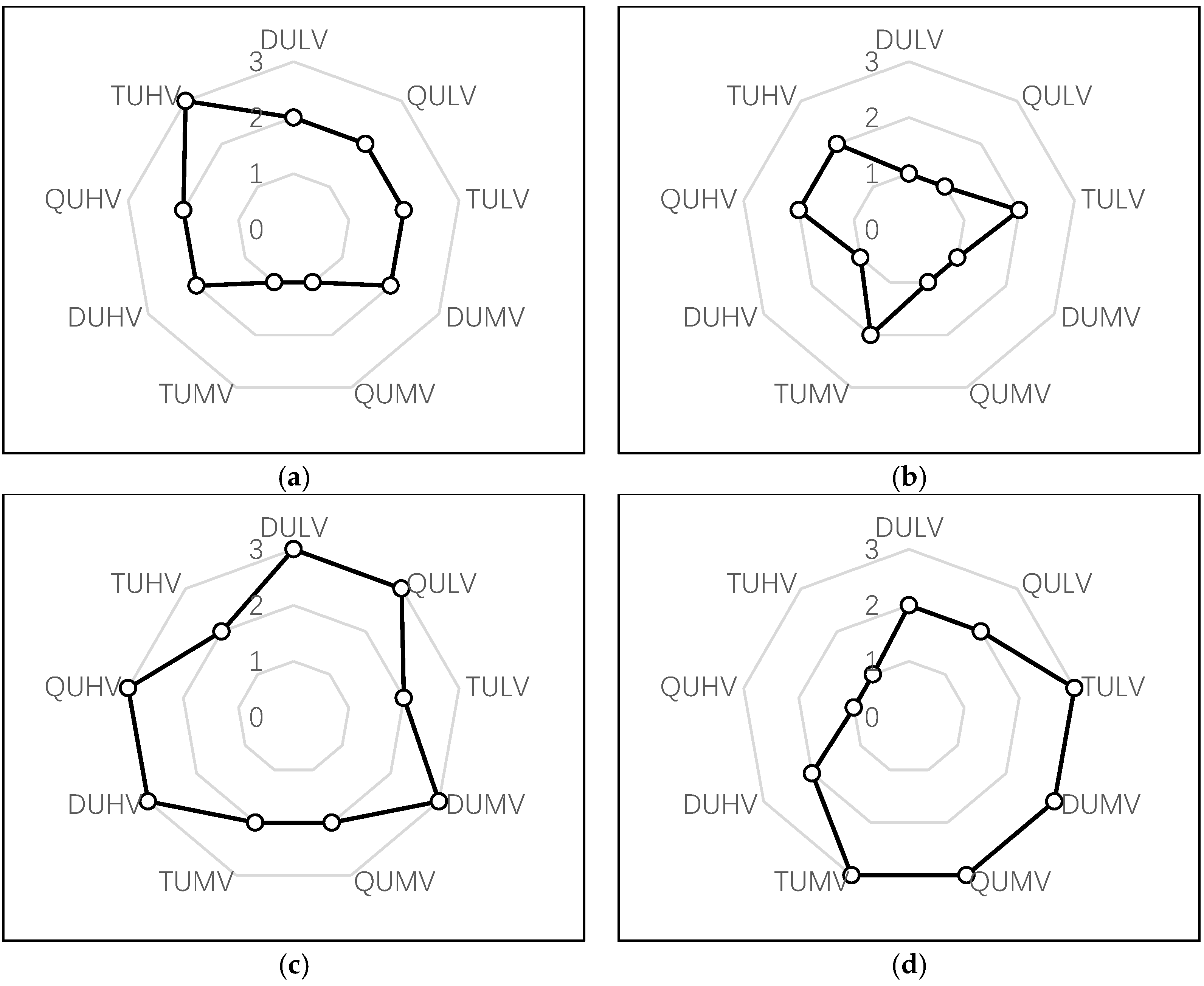
The performances of the proposed control strategies vary with the volume conditions. Figure 11 summarizes the performances under low volume (ULV), under moderate volume (UMV), and under high volume (UHV), relatively, with respect to the average stopped delay (D), queue length (Q), and vehicle throughput (T). The four uppercase letters in Figure 11 are the combination of indicators and volumes. For example, DULV means the average stopped delay under low volume, while QUHV is the queue length under high volume. In this figure, a point closer to the outer boundary indicates a better performance. In other words, the control strategy with a larger domain area covered by black lines and points has more potential to optimize the two-lane highway lane-closure work zone performance.
- Under Low volume
Compared with pre-timed control (Webster and Schonfeld), flagger control and actuated control show an advantage with respect to the average stopped delay, queue length, and vehicle throughput. The performance of flagger control is better than that of actuated control on average delay and queue length, but a bit worse on vehicle throughput. Pre-timed control proves to be the last alternative for two-lane highway work zones.
- Under Moderate volume
Instead of flagger control, actuated control gradually becomes superior to others, in terms of all the three traffic performance indicators. Flagger control, the best strategy when the volume is low, ranks second. The two pre-timed controls (Webster and Schonfeld) remain last, with the poorest performance.
- Under High volume
When the traffic volume rises to a high level, flagger control overtakes the others. Pre-timed control (Webster) ranks second, with the best performance on vehicle throughput. Pre-timed control (Schonfeld) is a little worse than pre-timed control (Webster) but outperforms actuated control. Actuated control becomes the worst on almost all the traffic performance indicators, except for average delay.
Note that when the vehicle inputs are close to or even exceed the capacity of two-lane highway work zones (namely, under oversaturated flow), the control plans generated by both flagger control and actuated control will be similar to those generated by pre-timed control. In this regard, the performance of the four control strategies should be close to each other. However, the performances of the four strategies are interesting: flagger control outperforms the two pre-timed controls, while actuated control is worse than pre-timed control. So when the traffic is over-saturated, flagger control strategy after optimization could be adopted as the best control strategy solution for two-lane highway work zones.
7.2. The Performance of Mathematical Stopped Delay Estimation
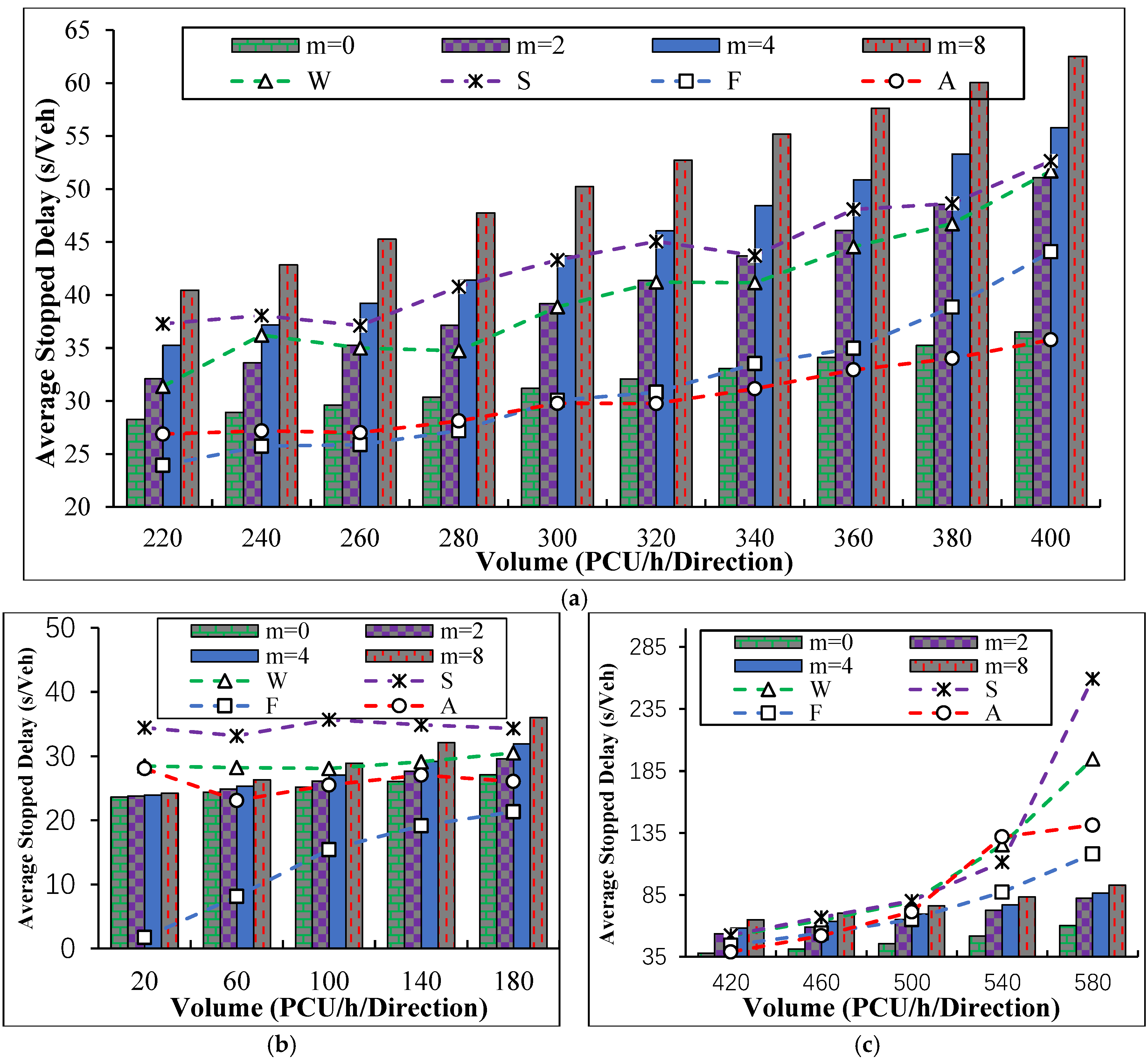
Except for the simulation model, the proposed mathematical model can be used for delay calculation under different control strategies with an appropriate value of parameter m. In this subsection, multiple different values of m (0, 2, 4, and 8) are tested. The results are summarized in Figure 12. In Figure 12, simulation results are represented by polylines, while the mathematical delay model calculation results are represented by histograms.
According to the figure, the trends from the mathematical model and simulation model results are generally consistent. When the volume is moderate, as shown in Figure 12a, all the simulation results are between the mathematical model estimations with m = 0 and m = 8. It is obvious that the mathematical models with proper values of m can describe the work zone control stopped delays under different kinds of control strategies. We can define the optimal mathematical model as the model that produces delay results closest to the simulated delays. However, multiple simulation results do not agree on a fixed, optimal m value. With the change of volume, the m for the optimal mathematical model may vary.
From Figure 12a, most m values are smaller than 8, the suggested value for signalized intersections in HCM 2010 [21]. However, in some other circumstances, larger values of m may be more suitable. When the volume is low, as shown in Figure 12b, the optimal m values are larger than under moderate volume. The stopped delays caused by pre-timed control (Schonfeld) even exceed the delay model predictions with m = 8. This indicates that the lower traffic volume can result in a higher degree of traffic flow randomness for work zones. In Figure 12c, when the volume is 500 PCU/h or more, the simulation results under all four control strategies are far bigger than the mathematical delay calculations. This is because of the existence of a maximum green time in the simulation environment that results in an additional queue delay.
From the previous analyses in Section 6.2, flagger control is the best with the smallest delays. No matter how small the value of m is, the proposed mathematical model is not capable of predicting the delay under the flagger control strategy when the traffic volume is smaller than 300 PCU/h. A more accurate mathematical delay model should be further studied for the two-lane highway work zone flagger control strategy.
8. Conclusions and Suggestions
This paper aimed to find better control strategies for two-lane highway lane-closure work zones with optimal average stopped delay, queue length, and vehicle throughput. Four control strategies including flagger control, pre-timed control proposed by Schonfeld, pre-timed control proposed by Webster, and actuated control were employed. Two primary methodologies, a mathematical delay model adopted from signalized intersections and a simulation model calibrated with field data were proposed. The results showed that control strategies for intersections can be used for two-lane highway work zones. Flagger control with optimal gap-out distance outperforms all the other control strategies under most traffic conditions. Actuated control, the most commonly used intersection control strategy, could be a good alternative for work zone areas due to its small queue length and large vehicle throughput under moderate-volume conditions.
From the simulation and mathematical results, six major suggestions for two-lane highway work zone control are summarized as follows:
- Flagger control after gap-out distance optimization is recommended due to the good performance of average delay, queue length, and throughput, especially under low- or high-volume conditions;
- Because optimal gap-out distance exists for flagger control, simulation can be employed to come up with the optimal value. A mark can be placed at the optimal gap-out distance ahead of the stop bar. When no vehicles run between the stop bar and the mark, flaggers can switch the paddle to the stop side;
- Actuated control, one of the most commonly used intersection control strategies, is a little bit worse than flagger control but outperforms pre-timed control. Under moderate-volume conditions, actuated control could be a good alternative for work zone areas due to its small queue length and large vehicle throughput;
- Although both of the pre-timed control strategies perform worst for two-lane work zones, they may still be used, as no additional devices (such as loop detectors) are required except for signal lights. After modification, Webster’s pre-timed control strategy is recommended for its better performance relative to Schonfeld’s method;
- Speed limit, as well as the average speed at work zone areas, can influence the performance of control strategies. With safety as the prerequisite, the average vehicle speed can be increased in the remaining lane. This is one general method to lower the stopped delay and queue length and to improve the vehicle throughput. In addition, the average speed needs to be controlled, and the speed limit should be determined carefully, although higher speed can reduce the vehicle delay. This is because higher speed means higher accident risk on one hand and because higher speeds will not result in significant delay reductions on the other hand.
- After calibration, the mathematical model can be used to describe the stopped delays under most of the work zone control strategies, except for under the flagger control method with low traffic volume conditions.
Nevertheless, this study can be enhanced in several ways in the future. Firstly, the conclusions are based on the field data collected from one work zone in 2013. More data should be collected to further test the performance of the four control strategies. Furthermore, the mathematical model is not suitable for flagger control delay estimation under a low traffic volume. A better mathematical delay model is needed for the flagger control strategy. Finally, Two-lane highway work zone length may also have an effect on delay time and the performance of control strategies, which remains to be studied in the future.
Author Contributions
The authors confirm contribution to the paper as follows: conceptualization, X.H. and Y.W.; methodology, X.H. and W.Z.; funding acquisition: X.H., Y.W. and W.W.; formal analysis, X.H.; writing—original draft preparation, X.H.; writing—review and editing, Y.W. and W.Y.
Funding
This work is supported by the National Natural Science of China (71801042, 51878166), the Natural Science of Jiangsu Province (BK20180381), and National Cooperative Highway Research Program, USA (03-107).
Conflicts of Interest
The authors declare no conflict of interest.
References
- Washington State DOT. Work Zone Safety. Available online: www.wsdot.wa.gov/safety/workzones/ (accessed on 15 April 2019).
- Ng, W.; Waller, T. A computationally efficient methodology to characterize travel time reliability using the fast Fourier transform. Transp. Res. Part B Methodol. 2010, 44, 1202–1219. [Google Scholar] [CrossRef]
- Debnath, A.K.; Blackman, R.A. Effectiveness of pilot car operations in reducing speeds in a long-term rural highway work zone. In Proceedings of the Transportation Research Board 93rd Annual Meeting, Washington, DC, USA, 5 February 2014. [Google Scholar]
- Chen, E.; Tarko, A.P. Modeling safety of highway work zones with random parameters and random effects models. Anal. Methods Accid. Res. 2014, 1, 86–95. [Google Scholar] [CrossRef]
- Wu, Z.; Sharma, A.; Mannering, F.L.; Wang, S. Safety impacts of signal-warning flashers and speed control at high-speed signalized intersections. Accid. Anal. Prev. 2013, 54, 90–98. [Google Scholar] [CrossRef] [PubMed]
- Adeli, H.; Jiang, X. Neuro-fuzzy logic model for freeway work zone capacity estimation. J. Transp. Eng. 2003, 129, 484–493. [Google Scholar] [CrossRef]
- Karim, A.; Adeli, H. Radial basis function neural network for work zone capacity and queue estimation. J. Transp. Eng. 2003, 129, 494–503. [Google Scholar] [CrossRef]
- Jiang, X.; Adeli, H. Object-Oriented model for freeway work zone capacity and queue delay estimation. Comput. Aided Civ. Infrastruct. Eng. 2004, 19, 144–156. [Google Scholar] [CrossRef]
- Weng, J.; Meng, Q. Estimating capacity and traffic delay in work zones: An overview. Transp. Res. Part C Emerg. Technol. 2013, 35, 34–45. [Google Scholar] [CrossRef]
- Meng, Q.; Weng, J. Optimal subwork zone operational strategy for short-term work zone projects in four-lane two-way freeways. J. Adv. Transp. 2013, 47, 151–169. [Google Scholar] [CrossRef]
- Pesti, G.; Jessen, D.R.; Byrd, P.S.; McCoy, P.T. Traffic flow characteristics of the late merge work zone control strategy. Transp. Res. Rec. J. Transp. Rese. Board 1999, 1657, 1–9. [Google Scholar] [CrossRef]
- Jiang, X.; Adeli, H. Freeway work zone traffic delay and cost optimization model. J. Transp. Eng. 2003, 129, 230–241. [Google Scholar] [CrossRef]
- Ng, M.; Lin, D.Y.; Waller, S.T. Optimal Long-Term Infrastructure Maintenance Planning Accounting for Traffic Dynamics. Comput. Aided Civ. Infrastruct. Eng. 2009, 24, 459–469. [Google Scholar] [CrossRef]
- Du, B.; Steven, I.; Chien, J. Feasibility of shoulder use for highway work zone optimization. J. Traffic Transp. Eng. 2014, 1, 235–246. [Google Scholar] [CrossRef] [Green Version]
- Zhu, W.; Li, Z.; Ash, J.; Wang, Y.; Hua, X. Capacity Modeling and Control Optimization for a Two-Lane Highway Lane-Closure Work Zone. J. Transp. Eng. 2017, 143, 04017059. [Google Scholar] [CrossRef]
- Mannion, P.; Duggan, J.; and Howley, E. An experimental review of reinforcement learning algorithms for adaptive traffic signal control. In Autonomic Road Transport Support Systems; Birkhäuser: Cham, Germeny, 2016; pp. 47–66. [Google Scholar]
- Araghi, S.; Khosravi, A.; Creighton, D. A review on computational intelligence methods for controlling traffic signal timing. Expert Syst. Appl. 2015, 42, 1538–1550. [Google Scholar] [CrossRef]
- Cheng, C.; Du, Y.; Sun, L.; Ji, Y. Review on theoretical delay estimation model for signalized intersections. Transp. Rev. 2016, 36, 479–499. [Google Scholar] [CrossRef]
- Hamilton, A.; Waterson, B.; Cherrett, T.; Robinson, A.; Snell, I. The evolution of urban traffic control: Changing policy and technology. Transp. Plan. Technol. 2013, 36, 24–43. [Google Scholar] [CrossRef]
- Dion, F.; Rakha, H.; Kang, Y.S. Comparison of delay estimates at under-saturated and over-saturated pre-timed signalized intersections. Transp. Res. Part B Methodol. 2004, 38, 99–122. [Google Scholar] [CrossRef]
- Transportation Research Board (TRB). Highway Capacity Manual; National Research Council: Washington, DC, USA, 2010. [Google Scholar]
- Ullman, G.L.; Levine, S.Z. An evaluation of portable traffic signals at work zones. Transp. Res. Rec. J. Transp. Res. Board 1987, 1148, 30–33. [Google Scholar]
- Chien, S.; Tang, Y.; Schonfeld, P. Optimizing work zones for two-lane highway maintenance projects. J. Transp. Eng. 2002, 128, 145–155. [Google Scholar] [CrossRef]
- Schonfeld, P.; Chien, S. Optimal work zone lengths for two-lane highways. J. Transp. Eng. 1999, 125, 21–29. [Google Scholar] [CrossRef]
- Finley, M.D.; Songchitruksa, P.; Jenkins, J. Evaluation of Alternative Methods of Temporary Traffic Control on Rural One-Lane, Twoway Highways; Texas A&M Transportation Institute: College Station, TX, USA, 2015. [Google Scholar]
- Ceder, A. An applicatoin of an optimal traffic control during lane closure periods of a two-lane road. J. Adv. Transp. 2000, 34, 173–190. [Google Scholar] [CrossRef]
- Cassidy, M.J.; Son, Y.; Rosowsky, D.V. Estimating motorist delay at two-lane highway work zones. Transp. Res. Part A Policy Pract. 1994, 28, 433–444. [Google Scholar] [CrossRef]
- Cassidy, M.J.; Han, L.D. Proposed model for predicting motorist delays at two-lane highway work zones. J. Transp. Eng. 1993, 119, 27–42. [Google Scholar] [CrossRef]
- Shibuya, S.; Nakatsuji, T.; Fujiwara, T.; Matsuyama, E. Traffic control at flagger-operated work zones on two-lane roads. Transp. Res. Rec. 1996, 1529, 3–9. [Google Scholar] [CrossRef]
- Ng, M. Traffic Flow Theory–Based stochastic optimization model for work zones on two-lane highways. J. Transp. Eng. 2012, 138, 1269–1273. [Google Scholar] [CrossRef]
- Chen, C.H.; Schonfeld, P.; Paracha, J. Work Zone Optimization for Two-Lane Highway Resurfacing Projects with an Alternate Route. Transp. Res. Rec. 2005, 1911, 51–66. [Google Scholar] [CrossRef]
- Chitturi, M.; Benekohal, R. Comparison of QUEWZ, FRESIM and QuickZone with field data for work zones. In Proceedings of the 83rd Transportation Research Board Annual Meeting, CD-ROM, Washington, DC, USA, 11–15 January 2004. [Google Scholar]
- Mitretek Systems. Quick Zone Delay Estimation Program, Version 2.0, User Guide; Federal Highway Administration: Washington, DC, USA, 2005.
- Washburn, S.; Hiles, T.; Kevin, H. Impact of Lane Closures on Roadway Capacity: Development of a Two-Lane Work Zone Lane Closure Analysis Procedure (Part A); Florida Department of Transportation: Tallahassee, FL, USA, 2008.
- Webster, F.V. Traffic Signal Settings; Road Research Technical Paper; Road Research Laboratory: London, UK, 1958. [Google Scholar]
- U.S. Department of Transportation. Manual on Uniform Traffic Control Devices (MUTCD); Federal Highway Administration: Washington, DC, USA, 2003.
- Klein, L.A.; Mills, M.K.; Gibson, D.R. Traffic Detector Handbook: Volume I; Turner-Fairbank Highway Research Center: Washington, DC, USA, 2006.
- Park, B.; Qi, H. Microscopic simulation model calibration and validation for freeway work zone network-a case study of VISSIM. In Proceedings of the 2006 IEEE Intelligent Transportation Systems Conference, Toronto, ON, Canada, 17–20 September 2006; pp. 1471–1476. [Google Scholar]
Figure 1.
Configuration of a typical work zone and an intersection: (a) work zone on a two-lane highway; and (b) a two-phase intersection.
Figure 1.
Configuration of a typical work zone and an intersection: (a) work zone on a two-lane highway; and (b) a two-phase intersection.

Figure 2.
Description of field data collection.

Figure 3.
Speed and headway on the two-lane highway work zone: (a) speed distribution; and (b) headway distribution.
Figure 3.
Speed and headway on the two-lane highway work zone: (a) speed distribution; and (b) headway distribution.

Figure 4.
Calculation result of the simulation model: (a) stopped delay based on different gap-out distance; and (b) percentage error (PE) of stopped delay.
Figure 4.
Calculation result of the simulation model: (a) stopped delay based on different gap-out distance; and (b) percentage error (PE) of stopped delay.

Figure 5.
Average stopped delay for different control strategies.

Figure 6.
Average stopped delay for different green extension times.

Figure 7.
Average stopped delay for different control strategies and volume: (a) under low volume; (b) under moderate volume; and (c) under high volume.
Figure 7.
Average stopped delay for different control strategies and volume: (a) under low volume; (b) under moderate volume; and (c) under high volume.


Figure 8.
Average stopped delay for different control strategies and speed.

Figure 9.
Queue length for different control strategies: (a) under low volume; (b) under moderate volume; and (c) under high volume.
Figure 9.
Queue length for different control strategies: (a) under low volume; (b) under moderate volume; and (c) under high volume.


Figure 10.
Difference between vehicle input and throughput: (a) under low volume; (b) under moderate volume; and (c) under high volume.
Figure 10.
Difference between vehicle input and throughput: (a) under low volume; (b) under moderate volume; and (c) under high volume.

Figure 11.
Radar maps of control performance under different volumes: (a) pre-timed control (Webster); (b) pre-timed control (Schonfeld); (c) flagger control; and (d) actuated control.
Figure 11.
Radar maps of control performance under different volumes: (a) pre-timed control (Webster); (b) pre-timed control (Schonfeld); (c) flagger control; and (d) actuated control.

Figure 12.
Mathematical and simulation delay estimations: (a) under moderate volume; (b) under low volume; and (c) under high volume.
Figure 12.
Mathematical and simulation delay estimations: (a) under moderate volume; (b) under low volume; and (c) under high volume.


Table 1.
Summary statistics of field data.
| Direction | Traffic Demand (veh/h) | Truck Percentage (%) | Speed Limit (Km/h) | Average Speed in Work Zone Area (Km/h) | Average Stopped Delay (s/veh) | Lane Changing Time (s) |
|---|---|---|---|---|---|---|
| 1 | 261 | 5.0 | 79.6 | 35.1 | 38.6 | 2.4/2.2 |
| 2 | 328 | 8.7 | 79.6 | 40.6 | 32.9 | - |
© 2019 by the authors. Licensee MDPI, Basel, Switzerland. This article is an open access article distributed under the terms and conditions of the Creative Commons Attribution (CC BY) license (http://creativecommons.org/licenses/by/4.0/).
Share and Cite
MDPI and ACS Style
Hua, X.; Wang, Y.; Yu, W.; Zhu, W.; Wang, W. Control Strategy Optimization for Two-Lane Highway Lane-Closure Work Zones. Sustainability 2019, 11, 4567. https://doi.org/10.3390/su11174567
AMA Style
Hua X, Wang Y, Yu W, Zhu W, Wang W. Control Strategy Optimization for Two-Lane Highway Lane-Closure Work Zones. Sustainability. 2019; 11(17):4567. https://doi.org/10.3390/su11174567
Chicago/Turabian StyleHua, Xuedong, YinHai Wang, Weijie Yu, Wenbo Zhu, and Wei Wang. 2019. "Control Strategy Optimization for Two-Lane Highway Lane-Closure Work Zones" Sustainability 11, no. 17: 4567. https://doi.org/10.3390/su11174567
Note that from the first issue of 2016, this journal uses article numbers instead of page numbers. See further details here.