Article

Decomposing Dynamics in the Farm Profitability: An Application of Index Decomposition Analysis to Lithuanian FADN Sample

by
Tomas Baležentis
*,
Aistė Galnaitytė
,
Irena Kriščiukaitienė
,
Virginia Namiotko
,
Lina Novickytė
,
Dalia Streimikiene
and
Rasa Melnikiene
Division of Farm and Enterprise Economics, Lithuanian Institute of Agrarian Economics, LT-03105 Vilnius, Lithuania
*
Author to whom correspondence should be addressed.
Sustainability 2019, 11(10), 2861; https://doi.org/10.3390/su11102861
Submission received: 12 April 2019 / Revised: 8 May 2019 / Accepted: 16 May 2019 / Published: 20 May 2019

Abstract

:
The changes in farm structure have been observed in Lithuania as well as in other Central and Eastern European countries. These changes, to a high extent, have been driven by decreasing profitability of the small farms. In this paper, we look into the changes in the profitability of Lithuanian family farms across different farm size groups. Farm size is measured in terms of the standard output. The period covered is 2005–2016. The index decomposition analysis model and Shapley value are adapted for the analysis. The proposed framework ensures complete decomposition among other desirable properties. The decomposition of the changes in profitability was carried out following the DuPont identity. The results suggest that for small (respectively large) farms the asset turnover (respectively profit margin) component appear more important, whereas the leverage effect remained minimal irrespectively of the farm size group.

1. Introduction

The increasing complexity of the agricultural policies and the role of the agricultural sector in the sense of viability of the rural areas have fuelled the need for integrated assessment frameworks for the agricultural sustainability [1,2,3,4]. Among different dimensions covered by the sustainability assessment frameworks, economic sustainability appears as an important facet [5,6]. Profitability level and its dynamics can be further considered as the key factors of economic sustainability.
Among multiple functions of the agricultural sector, the economic one is essential for maintaining its viability. In this regard, the measurement of income and profitability becomes a focal point in analysing performance of the agricultural sector [7]. More specifically, income level can indicate whether the farmers can sustain by embarking on the agricultural activities, whereas profitability indicates the attractiveness of investing into agricultural activities or, possibly, diverting investments into the other sectors. Therefore, it is important to measure the income and profitability of agricultural business. The dynamic analysis of the profitability is also important in the sense of identifying the major factors behind the changes in profitability [8]. The links between farm profitability and size demand further attention in the presence of structural dynamics.
The competitiveness of Central and Eastern European (CEE) agriculture has long been an important topic in agricultural economics literature [9,10]. Indeed, the latter region has seen collectivisation followed by post-communist transformations. The large-scale processes of de-collectivisation and the introduction of market economy have affected the paths and scale of agricultural development there. One of the most evident features of the CEE farming is the relatively small farm size (with certain exceptions in, e.g., Czech Republic). This induces a number of potential issues in regards to agricultural business viability. First, relatively small farms are often experiencing lower productivity levels if compared to large-scale farming due to insufficient access to credit markets, inability to exploit economies of scale, and complicated access to extension services. What is more, small farms often engage in mixed farming which further decreases productivity. Secondly, small farms may not generate enough income for farmer families which renders off-farm work and decrease the likelihood of passing the farm over to the next generation. Thirdly, small farms may face lower purchase prices which further dampers their profitability. However, this kind of agricultural structure does not induce excessive environmental burden as relatively low input intensity (especially, the use of agrochemicals) is maintained.
Anyway, large farms also face certain challenges in the CEE countries. The Common Agricultural Policy of the European Union offered access to Single Area Payment Scheme. This has caused a serious shift from livestock farming to crop farming and, particularly, cereal farming. Even though this strategy has allowed some farms to enjoy substantial income from sales and support payments, the production and market risk have both increased under the increasing specialization. In the wake of expansion of grain production in the Eastern Europe [11], the large cereal farms operating in CEE may also expect fluctuations in their competitiveness. Thus, the changes in farm structure are related to viability of the farming sector and this issue is even more topical in the CEE countries.
The changes in farm structure were observed in different CEE countries. For instance, Janovska et al. [12] showed that after the Czech Republic’s accession to the EU, the number of farms increased, whereas the average farm size decreased. The opposite pattern, however, was noticed in the other countries. Popescu et al. [13] found that during 2003–2013 the average farm size in Romania increased substantially and reached 3.66 ha of utilized agricultural area (UAA) at the end of the period. However, despite some positive changes, these researchers concluded that Romanian farms were still too small to be efficient. Similarly, Zdanovskis and Pilvere [14] showed that after Latvia’s accession to the European Union (EU) the number of farms with UAA exceeding 100 ha substantially increased. According to Lorber and Žiberna [15], similar trends were also documented in Slovenia, where the number of middle-sized and large farms increased during 2002–2012. Dannenberg and Kuemmerle [16] obtained similar results for Polish farms, whereas Latruffe et al. [17] arrived at the same conclusions after analyzing farm expansion in Lithuania after entry into the EU. Savickienė and Miceikienė [18] utilised the financial indicators to measure financial sustainability of Lithuanian farms. Krpalkova et al. [19] and Naglova and Gurtler [20] concluded that Czech small farms were the least profitable farms, while the best results were achieved by large farms. Similarly, Poczta and Średzińska [21] showed that Polish large farms were more profitable than small farms. Vasiliev et al. [22] identified the same patterns for Estonian farms. According to Wolf et al. [23], this relationship varied significantly throughout different stages of the economic cycle. However, Bojnec and Latruffe [24], after analysing the links between farm size, agricultural subsidies, and farm performance in Slovenia, observed a different pattern for Slovenian farms as small farms were more profitable than large farms. One of the key reasons for structural changes in CEE farming is the relatively low profitability of small farms (besides access to credit markets, institutional settings, investment potential, and other reasons; see [25,26,27]). Therefore, the changes in profitability of farms in the CEE countries may impact structural changes. Both profitability and structural change can be induced by the support policies. Accordingly, there is a need for developing the methodologies for analysis of profitability change and apply it for comparison of different farm size groups. The scientific problem addressed in this paper is the development of quantitative tools for identifying farm profitability change across different farm size groups.
In this paper, we focus on Lithuania which provides a case study of agricultural transformations in CEE. Lithuania‘s accession to the EU in 2004 triggered changes in all areas of the economy, including agriculture. The changes that have taken place in agriculture, to a high extent, were driven by increasing support payments under the EU Common Agricultural Policy (CAP) and intensifying competition from highly developed EU countries. The principal changes in agriculture during the said period were related to farm structure. Currently, the assessment of the links between farm size and profitability is particularly important. This is mainly due to the initiated EU-wide debate on the CAP support priorities beyond 2020 and the importance of the finding balance between support for smaller and larger farms. In this context, this paper aims to analyze the changes in the profitability of Lithuanian family farms across different farm size groups. The following tasks are therefore set: (1) to define the situation of Lithuanian farms in the EU context; (2) to present the methodology for analysis of the profitability change; and (3) to decompose the changes in the profitability of Lithuanian family farms across farm size groups. We carry out the decomposition analysis for different farm size groups so as to ascertain whether the magnitude of change and the drivers thereof vary across different farms size groups. Indeed, the structural change observed in the agricultural sector of Lithuania may be related to profitability change among other reasons. The research relies on the Farm Accountancy Data Network (FADN) which provides a unified accounting framework for farms across the EU Member States.
The paper proceeds as follows: Section 2 embarks on international comparison to identify the key trends in farm structure and performance across the selected countries. Section 3 presents the model for index decomposition analysis and data used. Section 4 discusses the results.

2. Lithuanian Farming in the EU Context

In order to identify the key trends prevailing in Lithuanian agriculture and compare these to those prevailing in the neighbouring countries, we apply the FADN database [28]. Note that the data presented in the latter database covers both family and corporate farms. Hence, this section does not differentiate between these two forms of farming. The data covering the period of 2005–2016 is used for the analysis.
The average indicators for 2005–2016 reflecting farm size in different EU countries are presented in Table 1. As one can note, CEE countries (Estonia, Lithuania, Latvia and Poland) exhibit much lower average farm size, especially if it measured in economic terms. As regards countries with a developed agricultural sector, the Netherlands, Denmark and Germany, the average farm economic size ranged in between 216 thousand EUR and 372 thousand EUR, whereas the same variable for the CEE countries ranged in between 24 thousand EUR and 73 thousand EUR. The differences in the UAA are present, yet not that certain. For the group of the developed agriculture countries, the average UAA stood in between 35 ha for the Netherlands and 93 ha for Denmark. As regards the CEE countries, the corresponding values ranged in between 18 ha for Poland and 122 ha for Estonia. The total output, net income, assets, and net worth considerable differ across the two groups of countries with the CEE countries falling much below the developed agriculture countries. The growth rates indicate a certain process of convergence in the average farm size as the CEE countries show much higher rates of growth than is the case for the developed agriculture countries (with certain exceptions for the UAA).
As suggested by the data on land productivity, the developed agriculture countries show much higher values if opposed to the CEE countries (Table 2). The Netherlands are exceptional in this regard due to their agricultural output structure (greenhouse farming). This is also related to differences in the asset intensity, where the CEE countries are much less asset-intensive in their farming if compared to the developed agriculture countries. This also implies farm modernization is a topical issue in the CEE countries. Turning to the rates of growth, the CEE countries tend to exhibit higher values (from 1.9% up to 4.6% for land productivity and from 3.3% up to 8.0% for asset intensity) as opposed to the developed agriculture countries (from 2.9% up to 3.7% and from 1.4% up to 3.5% respectively). Again, these figures suggest some sort of the underlying convergence. Given the relatively low asset levels, the CEE countries how excessively high return rates. However, this might be more a problem for valuation of the existing assets rather than indicator of the high farming productivity and, eventually, profitability (as the land productivity does not suggest the latter trend). In spite of featuring higher profitability rates, the CEE countries exhibit negative trends for these indicators (as contrasted to negligible change in the developed agriculture countries). This may be due to both increasing investments in assets and increasing pressure in the international agricultural markets which reduces the margins.
So far, we focused on the average farm size within specific countries. In order to further explore the trends in farm structure, we now turn to a more detailed analysis. Specifically, we look at the farm size within each economic size group across the selected counties. This allows identifying the prevailing farm structure and, to a certain extent, performance of farms. Thus, Table 3 brings forward the average UAA foe different farm size groups (as measured by the standard output). Besides simply looking at the average values, we also consider the differences in the average UAA between the two representative groups of the economic size so as to measure the degree of farm size inequality. More specifically, we choose farms producing output of 25–50 thousand EUR and those producing 500–750 thousand EUR as the relatively small and relatively large ones, respectively. Then, we look at the ratios of the average UAA for relatively large farms to that of the relatively small ones. Clearly, these ratios are much higher for the CEE countries if compared to the developed agriculture countries: the values for the CEE countries lies in between 799% for Estonia and 1290% for Latvia, whereas the corresponding interval for the developed agriculture countries is defined by 295% for the Netherlands and 586% for Germany. The latter finding implies that farm size inequality is much higher in the CEE countries if compared to those with developed agricultural sectors. Such a pattern suggests there have been serious expansion of large farms in the CEE countries which has been possibly driven by the CAP payments inducing a rather extensive mode of growth. What is more, it is important to ascertain whether profitability patterns are associated with structural dynamics.
In order to ascertain whether the differences in farm size inequality across different countries are due to differences in their competitiveness observed across different size groups or whether some external factors play a role there, we consider the land productivity. Again, we consider the difference between the two representative size groups in order to quantify the underlying inequality in land productivity. Even though there have been serious differences in inequality of farm size across the developed agriculture countries and CEE countries (Table 3 and Table 4) the inequality in land productivity is much the same across all the countries considered. This suggests that agricultural policies have also played an important role in shaping the farm structure in CEE countries. The values of the ratio exceed 100% which indicates smaller farms show lower land productivity in the selected countries.
The results (Table 4) indicate the CEE countries faced lower land productivity (from 722 EUR/ha up to 1398 EUR/ha) when compared to the developed agriculture countries (from 2600 EUR/ha up to 11883 EUR/ha). The profitability indicators, however, showed the opposite pattern. What is more, the profitability tended to decrease in the CEE countries. These findings call for further research into the dynamics of farm profitability in the CEE countries. In the sequel, we focus on the case of Lithuanian family farms.

3. Methods and Data

This section presents the analytical approach. First, we built an index decomposition analysis (IDA) identity relating the profitability (as measured by returns on assets) to the three explanatory variables unified under the DuPont model. Second, we related the variables of the FADN system to the IDA identity.
The DuPont model has been applied in different sectors to identify the underlying drivers of returns on equity [29]. The DuPont model allows for decomposing of the profitability. However, this was done for a certain time period. In order to move towards a dynamic setting, we further applied IDA and defined the decomposition of the changes in profitability. The proposed approach was operationalized via the Shapley value which ensures that several desirable properties of the underlying decomposition were met. Compared to such well-known models as growth accounting, we decomposed the change in profitability rather than output levels. Indeed, output (and productivity) growth does not necessarily lead to income and profitability growth.

3.1. IDA

The IDA allows quantifying the contributions of the different variables entering into a multiplicative relationship with a resulting variable. In our case, we defined the profitability indicator in terms of the DuPont identity thus arriving at a multiplicative structure. Methodologically, there have been the two major strands available for facilitating the IDA [30]: techniques built upon the Divisia index (e.g., LMDI) and those built upon the Laspeyres index (e.g., Shapley index). In this paper, we applied the Shapley value-based index which allows for path independency besides other desirable properties. This concept has been applied in addressing different economic problems [31].
Following Balezentis and Novickyte [8], we established the IDA identity linking return on equity to the three multiplicatively related terms (leverage, asset turnover, and profit margin). Therefore, profitability is explained in terms of integration in the credit markets, productivity of the assets, and marketing effectiveness. Mathematically, the following identity is used:
R t E t = R t Y t Y t A t A t E t = P t N t L t
where R refers to income, Y stands for output value, A is the asset value, E is the equity, P stands for profit margin, N represents asset turnover, L is the leverage ratio, and t denotes time period. Note that the ratio R / E gives the measure of returns to equity (ROE). Then, the IDA can be applied to decompose the change in the ROE. Assume we considered the two consecutive time periods, denoted by 0 and T :
Δ ( R E ) 0 , T = R T E T R 0 E 0 = Δ P + Δ N + Δ L
where Δ P , Δ N , and Δ L are the contributions to the change in ROE by the changes in the profit margin, asset turnover and leverage, respectively.
The Shapley value can then be employed to facilitate the decomposition given in Equation (2). Taking the three terms on the right-hand side of Equation (2) as an example, we have the following expression for an arbitrarily chosen term:
Δ i = s = 1 3 ( s 1 ) ! ( 3 s ) ! 3 ! S : x j S , | S | = s ( V ( S ) V ( S \ x i ) )
where S is the set of variables which change their levels going from period 0 to period T and V ( S ) = j S x j T j S x j 0 with j i for i = 1 , 2 , 3 . Thus, all the possible combinations of the elements of S are considered in order to appraise the marginal contribution of a certain term. In case the three terms are considered, the contribution of each of these is computed by considering the four possible instances of S associated with different weights as defined by Equation (3). Thus, the application of the Shapley value allowed decomposing of the change in the ROE indicator between any two time periods. In our case, we sought to decompose family farm profitability indicators in a chain-linked manner, i.e., by considering the annual changes between the two adjacent time periods. The next sub-section presents the data used for the empirical application.

3.2. Data Used

In order to facilitate the decomposition of profitability change for Lithuanian family farms, we applied the FADN database. The decomposition was carried for different farm size groups which are defined in terms of UAA (in ha) or farm economic size (standard output in EUR). Due to evolution of the FADN methodology, the data cover years 2005–2016 if farm size in UAA was considered or 2010–2016 in case economic farm size was considered.
The research relied on the FADN variables presented in Table 5. As one can note, the four absolute indicators represent income (Farm Net Income), output (total output), assets (total assets), and equity (net worth). The ROE was obtained by considering the ratio of income to equity. The absolute indicators can be used to construct the terms of Equation (1), i.e., profit margin, asset turnover, and leverage.

4. Results

The data and models presented in Section 3 allow quantifying the sources of changes in the farm profitability. In this section, we first look into the dynamics in the underlying variables across the farm size groups. Next, we present the results rendered by the IDA.

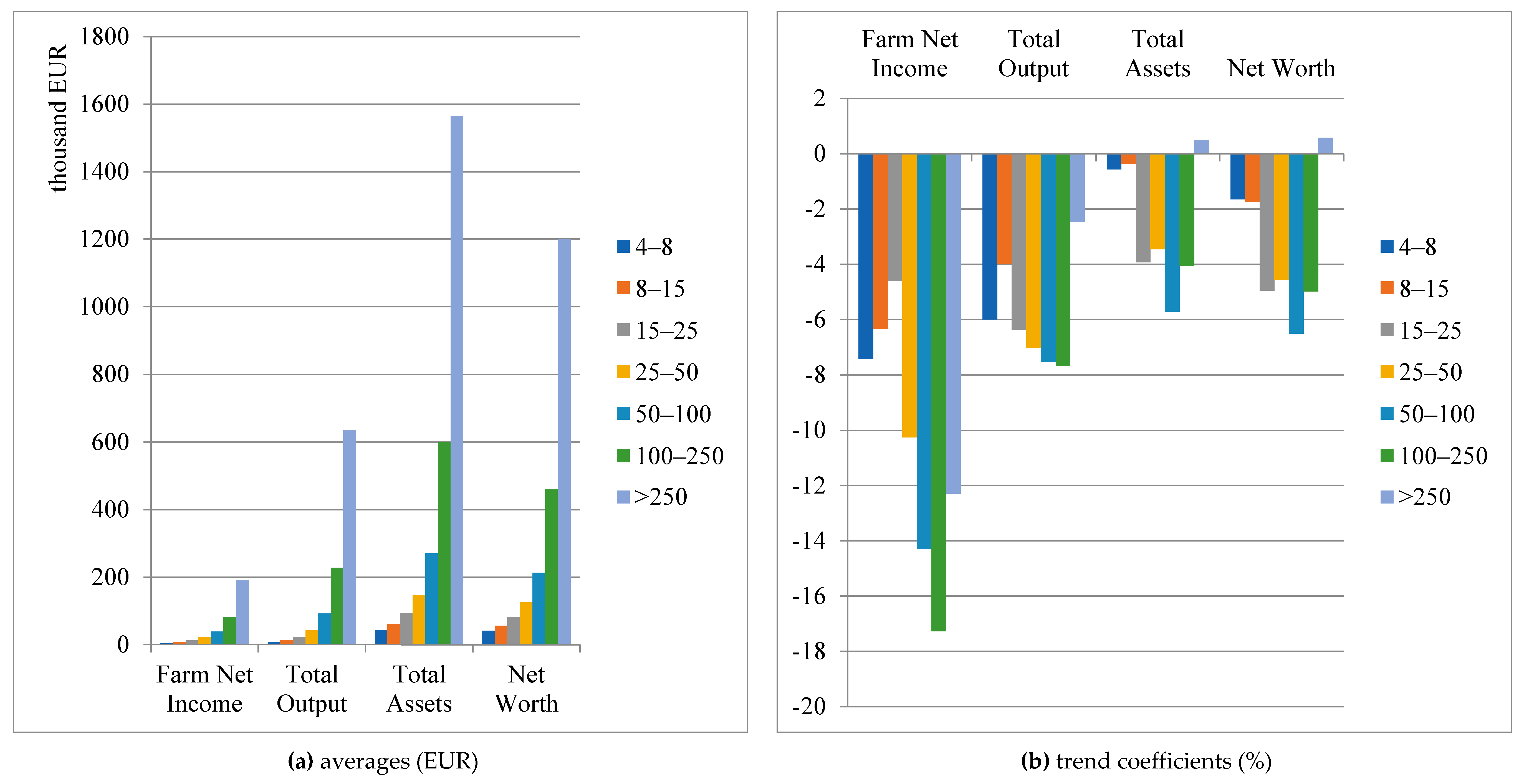
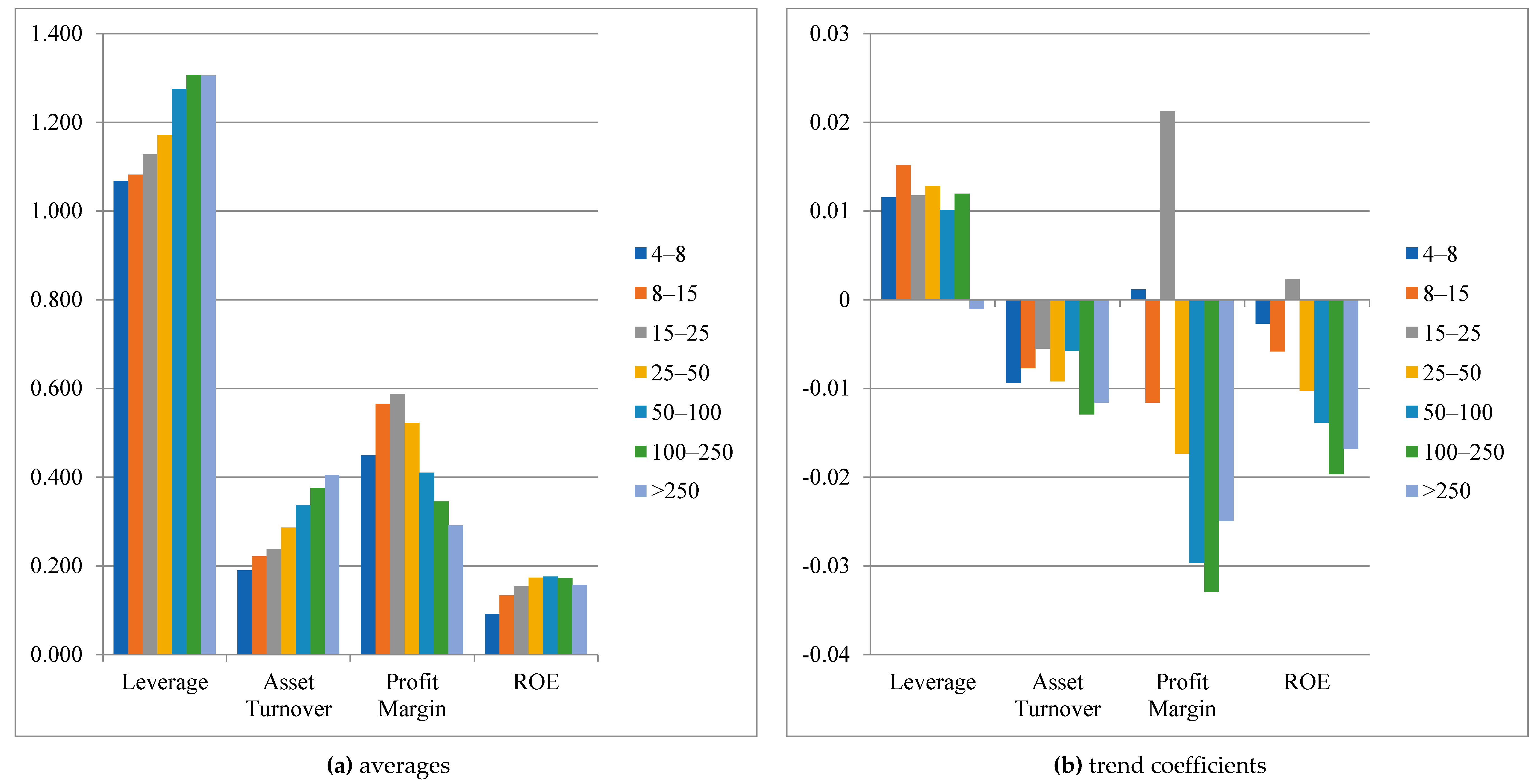
4.1. Financial Indicators
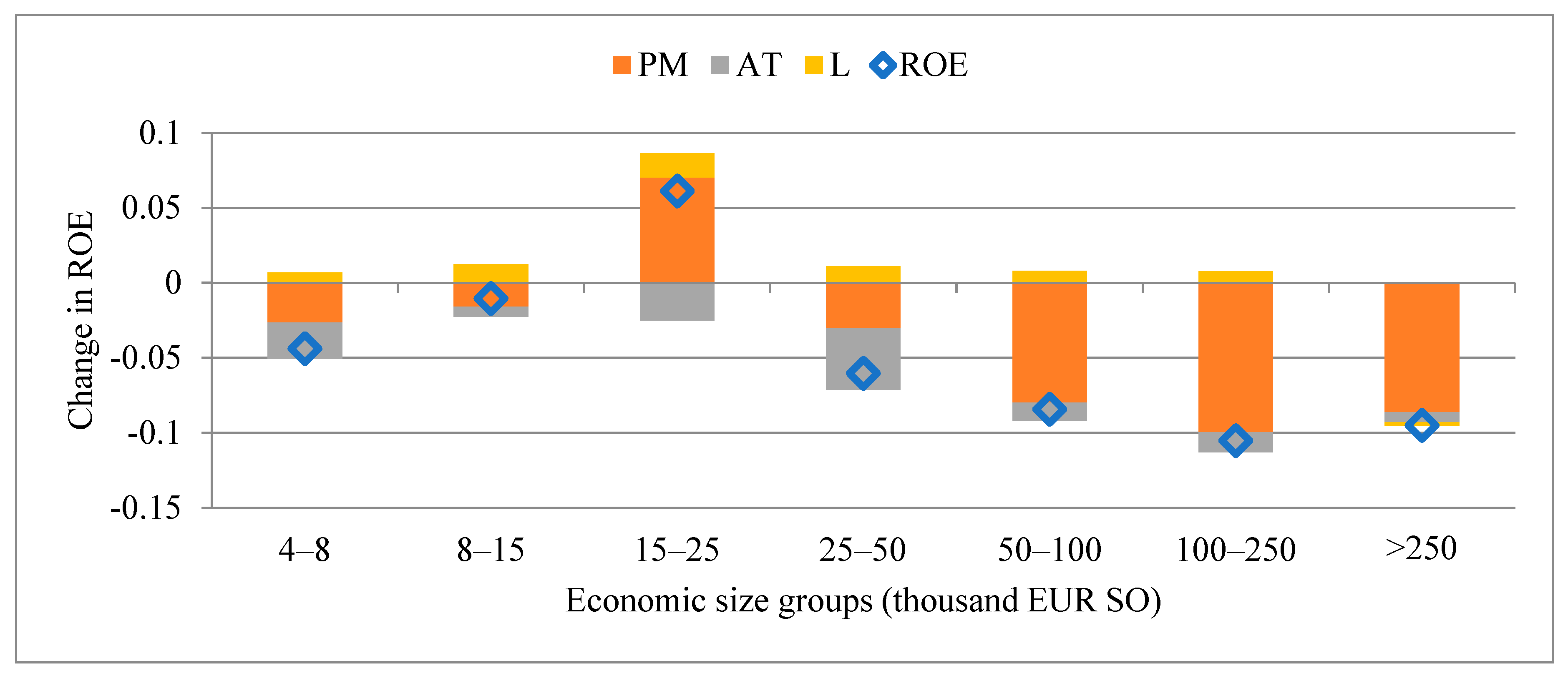
In this study, both absolute and relative financial indicators were considered in order to identify the underlying trends in profitability change. The farm size was measured in the sense of the economic size and UAA. The average values over the period covered and the trend coefficients were provided for each indicator and farm size group. This allowed identifying the actual situation along with possible change within each farm size group.
The financial indicators were given for the period of 2010–2016 for different economic size groups. The economic size was measured in terms of the standard output (SO). The absolute values of the financial indicators were increasing with farm size as expected (Figure 1a). As regards the changes in the absolute financial indicators, the trend coefficients revealed somewhat more interesting patterns (Figure 1b). Specifically, negative trends were observed for income, output assets, and equity indicators irrespectively of the farm size (with some minor exceptions for the largest farms). Even though the largest farms (with SO of more than 250 thousand) showed slightly positive trends in the absolute financial indicators, their output and income indicators still declined albeit at relatively lower pace. In general, the rate of decline in the absolute financial indicators decline with economic farm size.
The patterns observed for the relative financial indicators (Figure 2) were more complicated. The average leverage ratio increases with farm economic size (Figure 2a). This suggests larger farms tend to be more integrated with the credit markets and ensure appropriate capital structure. The average asset turnover also increases with farm size which is associated with higher productivity levels in the larger farms. However, the average profit margin decreases with economic farm size which indicates that larger farms do not necessarily generate profits from higher levels of outputs. This can be explained by a number of factors including diseconomies of scale or poor market integration due to support payments. The interactions of the enumerated terms resulted in an inverse U-shape relationship between the average ROE and economic farm size. Thus, the highest average ROE was observed for farms producing 50 to 100 thousand EUR.
Looking at the trends in the relative financial indicators provides some additional insights into farm performance across different economic size groups (Figure 2b). The dynamics in the leverage ratio does not differ across the economic farm size groups. In general, the leverage is increasing for all farm size groups. These findings suggest the differences in the leverage levels are likely to persist in the short run. The other relative indicators showed negative trends which calls for improvements in productivity and profitability. Asset turnover declines at a similar rate for all size groups. The rate of change in the profit margin and ROE varies across the farm size groups. Specifically, the rates of decline increase with farm size. This indicates that the largest farms are likely to face serious profitability decline besides already low level of the profit margin.
As one can note, the terms of the DuPont identity moved towards different directions. Furthermore, certain differences have been observed across the farming types. In the next section, we apply the Shapley value to attribute the changes in the terms of DuPont model.

4.2. IDA

In order to quantify the effects of the terms comprising the DuPont identity and interacting simultaneously, we applied the IDA model based on the Shapley value as described in Section 3.1. The analysis was carried out in a chain-linked setting and then the results were aggregated for the whole period of 2010–2016. The results are presented in Figure 3.
The general trend is that the changes in the ROE decrease with farm size (this was already shown in Figure 2a in a stochastic manner). The profit margin appears as the major driver of the change in profitability. However, the asset turnover plays an important role for smaller farms. For instance, the ROE declined by 4.4 p.p. for the smallest farms (4 to 8 thousand EUR SO) out of which the parts of decline of 2.7 p.p. and 2.4 p.p. were due to changes in the profit margin and asset turnover, respectively. The remaining part of the overall change in ROE was explained by an increase in the ROE due to the leverage effect by 0.7 p.p. which was offset by the former two effects. The similar pattern was observed for farms falling within the 25 to 50 thousand EUR SO category. However, in the latter case, the effect of the asset turnover dominated (decline by 4 p.p.) over the profit margin effect (decline by 3 p.p.). The farm group corresponding to 15–25 thousand EUR SO shows an increase in ROE which does not follow the patterns observed for either smaller or larger farms. This group of farms includes relatively more productive milk farms and cereal farms (including rape-growing farms). Note that the milk selling prices are highly variable across the farms size groups in Lithuania [32]. These farms face higher yields and selling prices if opposed to the groups of smaller economic size this is confirmed by the higher profit margin gains in Figure 2b).
The largest farms (more than 50 thousand EUR SO) show the similar patterns in regards to the change in ROE. Specifically, much of the change in the ROE is due to the profit margin, whereas the effects of the leverage and asset turnover are less important. Note that farms falling within the group of over 250 thousand EUR SO do not improve their ROE due to the changes in the leverage.
The decline in the ROE observed for almost all farm size groups can be attributed to unfavourable market conditions. Table 6 presents the dynamics in price scissors for agriculture in Lithuania during 2010–2016. As one can note, input prices went up during 2010–2015 and declined during 2015–2016. The resulting increase in the input prices over the period of 2010–2016 is 2.8%. The prices of crop output went up in general (1.7% over 2010–2016) and those of livestock output declined by some 6.1%. The combined agricultural output index indicates a decline in the output prices of 2.7%. Irrespectively of the output type considered, the price scissor indicators for 2014–2016 fall below 100% suggesting that growth rates in the input prices exceeded those in the output prices. The crop farms saw favourable situation in the sense of the price scissors during 2011–2013, yet livestock farms still faced increasing price scissors for 2011–2012. Therefore, situation in the agricultural markets suppressed the growth in profitability of Lithuanian family farms.
Access to the credit markets also impact the factor allocation and intensity on farms [33,34]. Furthermore, subsidised loans have an effect on the investment behaviour [35]. In this context, the relatively low leverage for small farms in Lithuania does not allow for transition towards less labour-intensive farming practices. Indeed, Petrick [35] reported the negative link between investment and farm size thus suggesting the need for lending policies which would encourage the small farms to improve their input structure and farming practices in general. These findings generally apply for the Lithuanian case. Anyway, there is a slightly positive contribution of leverage towards the ROE growth reported for most of the farm size groups with exception for the largest farms (Figure 3). Especially, the farm size group of 15–25 thousand EUR SO shows the highest increase in the ROE due to the leverage factor. This group includes milk farms which could have received investment support for modernisation.
The largest contributions of the asset turnover change towards the decline in the ROE are observed for relatively small farms (4–8 thousand EUR SO and 15–50 thousand ha SO). This indicates that the leverage and resulting investments might have not improved the output levels to a substantial extent in those farms. Therefore, there have violations of the optimal level of investments or type of capital goods acquired in Lithuanian family farms. However, the market conditions need to be taken into account when deciding on investments and lending as large quantities of non-marketed outputs would not contribute to increase in revenue and profitability. This seems to be a problem for large Lithuanian family farms (over 50 thousand EUR SO) as suggested by Figure 3. In this regard, support policies should aim to adjust the output mix and encourage more efficient use of inputs in the large farms.

5. Conclusions

This paper proposed a framework for decomposition of the farm profitability with particular focus on the farm size. The case of Lithuania was considered as an instance of the agricultural sector facing transformations following post-communist transformations and EU CAP. The FADN was applied for the analysis. Different farm size groups were defined in terms of the standard output. The index decomposition analysis based on the Shapley value was employed in order to quantify the contributions of the different terms of profitability unified under the DuPont model.
The results indicate that small Lithuanian family farms are less profitable than the large ones in general (as measured by the ROE ratio). The trends of changes in ROE are negative for all farm size groups. However, the trends in profitability suggest a certain possibility of convergence as the larger farms tend to face higher rates of decline in ROE if compared to the smaller farms.
Application of the Shapley value allowed to perform the decomposition of the changes in the ROE and attribute these to the changes in profit margin, asset turnover, and leverage. The results indicate leverage is rather low for small farms thus indicating low integration into credit markets. The decomposition showed its contribution to the changes in the ROE is also minimal. Thus, the profitability of the equity could be increased by properly managing the financial structure of the farms (in cases where profitable production is possible). In this regard, support policies should aim at implementing risk mitigation measures and improving the extension services. The profitability should be maintained by improving marketability of the farm production.
Decline in profitability of Lithuanian family farms shows increasing extent with farm size. For small (respectively large) farms, the asset turnover (respectively profit margin) component appeared more important, whereas the leverage effect remained minimal irrespective of the farm size group. Therefore, the changes in productivity are more important for the smaller farms. This requires further modernization with proper balance between own and borrowed capital. For the large farms, more attention towards improved marketing strategies should be paid. The increasing labour costs undoubtedly reduce the profitability of large farms which rely on hired labour force. Among other reasons, the CAP payments in Lithuania may distort incentives for higher market integration and, thus, profit margins in the large farms due to unlimited area payments. The changes in price scissors indicated unfavourable dynamics in the agricultural input and output prices in Lithuania. These have dampened the profitability change, especially via the profit margin component. This suggests that risk management tools are needed for Lithuanian family farms in order to mitigate income loss due to the market fluctuations.
Regarding farm sustainability and viability in Lithuania, results of the study suggest that further expansion of large farms may have diverse effects. As the large farms enjoy higher levels of profitability, the shift towards large-scale farming may induce increase in the profitability in the short-run and medium-run. However, the trends in profitability suggest that the large farms exhibit higher rates for decline which implies a long-run decline in the profitability. This requires streamlining credit financing and investment decisions along with adjustment of output-mix and marketing strategies in order to ensure improvements in farm profitability and sustainability. Besides the economic considerations, one should also take into account more intensive farming practices prevailing in the large farms which result in increased environmental pollution.
This study relies on the aggregate data. Further studies could aim at exploiting the farm-level data. This would allow for farm-level analysis of profitability change and identification of the determinants of profitability change. In addition, the production theory could be employed to analyse farm profitability in the productivity accounting framework.

Author Contributions

Data curation, A.G. and L.N.; Methodology, I.K.; Writing—original draft, T.B. and V.N.; Writing—review & editing, D.S. and R.M.

Funding

This research is funded by the European Social Fund according to the activity “Improvement of researchers’ qualification by implementing world-class R&D projects” of Measure No. 09.3.3-LMT-K-712.

Conflicts of Interest

The authors declare no conflict of interest.

References

  1. Meul, M.; Van Passel, S.; Nevens, F.; Dessein, J.; Rogge, E.; Mulier, A.; Van Hauwermeiren, A. MOTIFS: A monitoring tool for integrated farm sustainability. Agron. Sustain. Dev. 2008, 28, 321–332. [Google Scholar] [CrossRef]
  2. Zahm, F.; Viaux, P.; Vilain, L.; Girardin, P.; Mouchet, C. Assessing farm sustainability with the IDEA method–from the concept of agriculture sustainability to case studies on farms. Sustain. Dev. 2008, 16, 271–281. [Google Scholar] [CrossRef]
  3. Kelly, E.; Latruffe, L.; Desjeux, Y.; Ryan, M.; Uthes, S.; Diazabakana, A.; Dillon, E.; Finn, J. Sustainability indicators for improved assessment of the effects of agricultural policy across the EU: Is FADN the answer? Ecol. Indic. 2018, 89, 903–911. [Google Scholar] [CrossRef]
  4. Repar, N.; Jan, P.; Nemecek, T.; Dux, D.; Doluschitz, R. Factors affecting global versus local environmental and economic performance of dairying: A case study of Swiss mountain farms. Sustainability 2018, 10, 2940. [Google Scholar] [CrossRef]
  5. Lien, G.; Hardaker, J.B.; Flaten, O. Risk and economic sustainability of crop farming systems. Agric. Syst. 2007, 94, 541–552. [Google Scholar] [CrossRef] [Green Version]
  6. Zorn, A.; Esteves, M.; Baur, I.; Lips, M. Financial Ratios as Indicators of Economic Sustainability: A Quantitative Analysis for Swiss Dairy Farms. Sustainability 2018, 10, 2942. [Google Scholar] [CrossRef]
  7. Czyżewski, B.; Matuszczak, A.; Miśkiewicz, R. Public goods versus the farm price-cost squeeze: shaping the sustainability of the EU’s common agricultural policy. Technol. Econ. Dev. Econ. 2019, 25, 82–102. [Google Scholar] [CrossRef]
  8. Balezentis, T.; Novickyte, L. Are Lithuanian Family Farms Profitable and Financially Sustainable? Evidence Using DuPont Model, Sustainable Growth Paradigm and Index Decomposition Analysis. Transform. Bus. Econ. 2018, 17, 237–254. [Google Scholar]
  9. Gorton, M.; Davidova, S. Farm productivity and efficiency in the CEE applicant countries: A synthesis of results. Agric. Econ. 2004, 30, 1–16. [Google Scholar] [CrossRef]
  10. Henningsen, A. Why is the Polish farm sector still so underdeveloped? Post-Communist Econ. 2009, 21, 47–64. [Google Scholar] [CrossRef]
  11. Swinnen, J.; Burkitbayeva, S.; Schierhorn, F.; Prishchepov, A.V.; Müller, D. Production potential in the “bread baskets” of Eastern Europe and Central Asia. Glob. Food Secur. 2017, 14, 38–53. [Google Scholar] [CrossRef]
  12. Janovska, V.; Simova, P.; Vlasak, J.; Sklenicka, P. Factors affecting farm size on the European level and the national level of the Czech Republic. Agric. Econ. (Zemědělská Ekonomika) 2017, 63, 1–12. [Google Scholar] [Green Version]
  13. Popescu, A.; Alecu, I.N.; Dinu, T.A.; Stoian, E.; Condei, R.; Ciocan, H. Farm Structure and Land Concentration in Romania and the European Union’s Agriculture. Agric. Agric. Sci. Procedia 2016, 10, 566–577. [Google Scholar] [CrossRef]
  14. Zdanovskis, K.; Pilvere, I. Agricultural development in Latvia after joining the European Union. Res. Rural Dev. 2015, 2, 161–168. [Google Scholar]
  15. Lorber, L.; Žiberna, I. European Agricultural Policy and Structural Changes in Agricultural Holdings in Podravje between 2002–2012. Podrav. Čas. za Multidiscip. Istraživanja 2014, 13, 19–44. [Google Scholar]
  16. Dannenberg, P.; Kuemmerle, T. Farm size and land use pattern changes in postsocialist Poland. Prof. Geogr. 2010, 62, 197–210. [Google Scholar] [CrossRef]
  17. Latruffe, L.; Davidova, S.; Douarin, E.; Gorton, M. Farm expansion in Lithuania after accession to the EU: The role of CAP payments in alleviating potential credit constraints. Eur.-Asia Stud. 2010, 62, 351–365. [Google Scholar] [CrossRef]
  18. Savickienė, J.; Miceikienė, A. Sustainable economic development assessment model for family farms. Agric. Econ. Czech 2018, 64, 527–535. [Google Scholar] [CrossRef]
  19. Krpalkova, L.; Cabrera, V.E.; Kvapilik, J.; Burdych, J. Dairy farm profit according to the herd size, milk yield, and number of cows per worker. Agric. Econ. (Zemědělská Ekonomika) 2016, 62, 225–234. [Google Scholar] [CrossRef] [Green Version]
  20. Naglova, Z.; Gurtler, M. Consequences of supports to the economic situation of farms with respect to their size. Agric. Econ. (Zemědělská Ekonomika) 2016, 62, 311–323. [Google Scholar] [Green Version]
  21. Poczta, W.; Średzińska, J. Wyniki produkcyjno-ekonomiczne i finansowe indywidualnych gospodarstw rolnych według ich wielkości ekonomicznej (na przykładzie regionu FADN Wielkopolska i Śląsk). Probl. World Agric. 2007, 2, 433–443. [Google Scholar]
  22. Vasiliev, N.; Astover, A.; Roostalu, H.; Matvejev, E. An agro-economic analysis of grain production in Estonia after its transition to market economy. Agron. Res. 2006, 4, 99–110. [Google Scholar]
  23. Wolf, C.A.; Stephenson, M.W.; Knoblauch, W.A.; Novakovic, A.M. Dairy farm financial performance: Firm, year, and size effects. Agric. Financ. Rev. 2016, 76, 532–543. [Google Scholar] [CrossRef]
  24. Bojnec, Š.; Latruffe, L. Farm size, agricultural subsidies and farm performance in Slovenia. Land Use Policy 2013, 32, 207–217. [Google Scholar] [CrossRef]
  25. Zimmermann, A.; Heckelei, T. Structural change of European dairy farms—A cross-regional analysis. J. Agric. Econ. 2012, 63, 576–603. [Google Scholar] [CrossRef]
  26. Breustedt, G.; Glauben, T. Driving forces behind exiting from farming in Western Europe. J. Agric. Econ. 2007, 58, 115–127. [Google Scholar] [CrossRef]
  27. Zimmermann, A.; Heckelei, T.; Domínguez, I.P. Modelling farm structural change for integrated ex-ante assessment: Review of methods and determinants. Environ. Sci. Policy 2009, 12, 601–618. [Google Scholar] [CrossRef]
  28. European Commission. FADN Public Database. Available online: http://ec.europa.eu/agriculture/rica/database/database_en.cfm (accessed on 1 April 2019).
  29. Soliman, M.T. The use of DuPont analysis by market participants. Account. Rev. 2008, 83, 823–853. [Google Scholar] [CrossRef]
  30. Ang, B.W.; Huang, H.C.; Mu, A.R. Properties and linkages of some index decomposition analysis methods. Energy Policy 2009, 37, 4624–4632. [Google Scholar] [CrossRef]
  31. Aristondo, O.; Onaindia, E. On measuring the sources of changes in poverty using the Shapley method. An application to Europe. Fuzzy Sets Syst. 2018. [Google Scholar] [CrossRef]
  32. Stalgiene, A.; Jedik, A.; Viira, A.H.; Krievina, A. Market Power in Lithuanian, Latvian and Estonian Dairy Sectors: The Case of Raw Milk Market. Transform. Bus. Econ. 2017, 16, 89–105. [Google Scholar]
  33. Ciaian, P.; Fałkowski, J.; Kancs, D.A. Access to credit, factor allocation and farm productivity: Evidence from the CEE transition economies. Agric. Financ. Rev. 2012, 72, 22–47. [Google Scholar] [CrossRef]
  34. Pandey, B.; Bandyopadhyay, P.; Kadam, S.; Singh, M. Bibliometric study on relationship of agricultural credit with farmer distress. Manag. Environ. Qual. 2018, 29, 278–288. [Google Scholar] [CrossRef]
  35. Petrick, M. Farm investment, credit rationing, and governmentally promoted credit access in Poland: A cross-sectional analysis. Food Policy 2004, 29, 275–294. [Google Scholar] [CrossRef]
Figure 1. Absolute financial indicators for Lithuanian family farms (by standard output (SO) groups, measured in thousand EUR), 2010–2016. Note: averages are computed as the arithmetic averages over 2010–2016, whereas the trend coefficients represent average annual growth rates (in per cent).
Sustainability 11 02861 g001
Figure 2. Financial ratios for Lithuanian family farms (by SO groups, measured in thousand EUR), 2010–2016. Note: averages are computed as the arithmetic averages over 2010–2016, whereas the trend coefficients represent average annual rates of change (in percentage points).
Sustainability 11 02861 g002
Figure 3. Decomposition of the cumulative change in the ROE for Lithuanian family farms across economic size groups, 2010–2016. Note: results of the adjacent time periods (i.e., chain-linked analysis) are added up to obtain the cumulative change.
Sustainability 11 02861 g003
Table 1. Farm size indicators for selected EU countries, 2005–2016.
CountryEconomic Size,
1000 EUR
Total Utilised Agricultural Area, haTotal Output, EURFarm Net Income, EURTotal Assets, EURNet Worth, EUR
Average
Netherlands372.435.3422,16751,3842,065,9951,335,299
Denmark295.993.3371,05312,0282,354,6371,026,715
Germany216.284.0219,57336,877813,050651,501
Estonia73.2121.688,89214,549223,024152,735
Lithuania23.443.731,60012,74399,40484,683
Latvia33.966.447,67211,801119,34580,992
Poland24.218.426,7278646132,633123,326
Annual Rate of Growth (%)
Netherlands4.01.35.06.24.85.1
Denmark5.31.74.86.83.62.1
Germany1.91.54.42.72.92.2
Estonia6.72.47.0-3.97.86.7
Lithuania7.03.67.11.67.06.3
Latvia4.60.74.60.66.36.2
Poland4.10.52.41.88.59.1
Note: Arithmetic averages for 2005–2016 are provided. Rates of growth are based on the stochastic trend.
Table 2. Relative indicators for selected European Union (EU) countries, 2005–2016.
CountryLand Productivity, EUR/haAsset Intensity, EUR/haROA, %ROE, %
Averages
Netherlands11,88358,1832.53.8
Denmark395125,1080.61.4
Germany260096564.55.6
Estonia72218097.410.4
Lithuania710224113.215.3
Latvia718179410.415.3
Poland144771677.07.6
Annual Rates of Growth (%)Annual Rates of Change (p.p.)
Netherlands3.73.50.00.0
Denmark3.11.80.10.2
Germany2.91.40.00.0
Estonia4.65.4−0.9−1.3
Lithuania3.53.3−0.7−0.7
Latvia3.95.6−0.6−0.9
Poland1.98.0−0.5−0.6
Table 3. Average utilized agricultural area (UAA) across different economic size groups in selected EU countries, 2005–2016.
Economic SizeNetherlandsDenmarkGermanyEstoniaLithuaniaLatviaPoland
(03) 4000–8000 EUR 21.816.224.07.8
(04) 8000–15,000 EUR 34.226.833.711.6
(05) 15,000–25,000 EUR 20.7 52.646.050.617.2
(06) 25,000–50,000 EUR15.535.028.894.076.383.226.6
(07) 50,000–100,000 EUR21.761.539.6172.3142.2159.245.0
(08) 100,000–250,000 EUR32.599.667.5335.6286.8324.079.7
(09) 250,000–500,000 EUR46.9137.5109.8626.1586.4673.4204.0
(10) 500,000–750,000 EUR45.8176.9168.8751.0854.11072.9334.8
(11) 750,000–1,000,000 EUR46.5209.5250.1933.21154.3 491.6
(12) 1,000,000–1,500,000 EUR40.0249.8423.01185.1 695.5
(13) 1,500,000–3,000,000 EUR33.7333.51010.51682.71539.4 1460.0
(14) ≥3,000,000 EUR29.6345.61729.4
Average35.393.384.0121.643.766.418.4
Ratio (10)/(6), %295506586799112012901260
Note: Arithmetic averages for 2005–2016 are provided.
Table 4. Average land productivity in selected EU countries, 2005–2016.
Total Output Per ha, Eur/haNetherlandsDenmarkGermanyEstoniaLithuaniaLatviaPoland
(03) 4000–8000 EUR 519375831
(04) 8000–15,000 EUR 379504394902
(05) 15,000–25,000 EUR 3498 3555015561042
(06) 25,000–50,000 EUR6037283316943995785231321
(07) 50,000–100,000 EUR6033280320815106585731594
(08) 100,000–250,000 EUR6484245025885467977002046
(09) 250,000–500,000 EUR84573315315472288110192294
(10) 500,000–750,000 EUR14,00440993235 1127 3209
(11) 750,000–1,000,000 EUR20,13546473093 1193 1810
(12) 1,000,000–1,500,000 EUR35,88053142584 2504
(13) 1,500,000–3,000,000 EUR70,42961912026 1993 1925
(14) ≥3,000,000 EUR238,168 2651
Average11,883395126007227107181398
Ratio (10)/(6)232145191181195195243
Note: Ratio (9)/(6) is used for Latvia and Estonia due to data availability. Arithmetic averages for 2005–2016 are provided.
Table 5. Data used in the Farm Accountancy Data Network (FADN) system.
IndicatorFADN Variable
Financial Indicators
Farm Net Income, EURSE420
Total output, EURSE131
Total assets, EURSE436
Net worth, EURSE501
Relative Indicators
Profit margin (P)SE420/SE131
Asset turnover (N)SE131/SE436
Leverage (L)SE436/SE501
Return on Equity (ROE)SE420/SE501
Farm Size Indicators
Economic size, EURSE005
Total Utilised Agricultural Area, haSE025
Table 6. Price scissors for agricultural production in Lithuania, 2010–2016.
YearInput Price IndexOutput Price IndexPrice Scissors
CropLivestockCombinedCropLivestockCombined
2010100100100100100100100
2011119137.5113.3123.8115.595.2104.0
2012126.3133.6115.2123.1105.891.297.5
2013119.3129.7123.5126.2108.7103.5105.8
2014115.6110.3111.4110.995.496.495.9
2015117.9109.795101.393.080.685.9
2016102.8101.793.997.398.991.394.6
Note: input price index for currently consumed inputs is provided; the nominal price indices are used; the data come from Eurostat.

