Integrating Cellular Automata with Unsupervised Deep-Learning Algorithms: A Case Study of Urban-Sprawl Simulation in the Jingjintang Urban Agglomeration, China


Abstract
:1. Introduction
2. Methodology
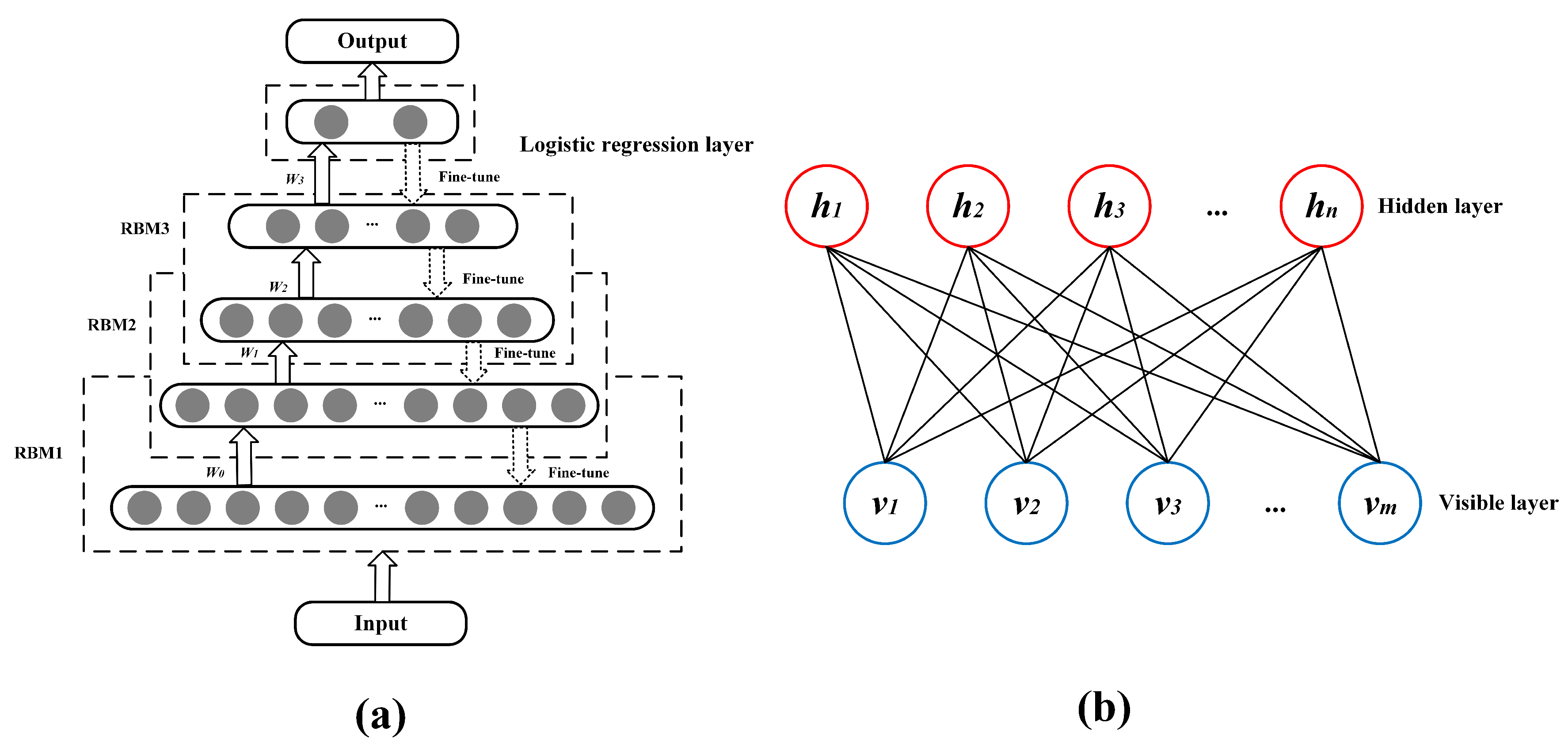
2.1. DBN
- Unsupervised pretraining stage: (1) Train the bottom RBM with CD on training data v being the visible units; (2) freeze weights matrix W and bias a, b of the first RBM, and the state of the hidden units is inferred and used as the input of the next higher RBM; (3) next higher RBM is stacked on top of the previous lower RBM after training; (4) iterate Steps 2 and 3 for the desired number of layers, each time upward propagating either samples or mean values.
- Supervised fine-tuning stage: After an unsupervised pretraining stage, all parameters need to be slightly adjusted in supervised manner until DBN loss function reaches its minimum. In this paper, a logistic regression layer periodically works in the top-level RBM during the supervised fine-tuning stage.
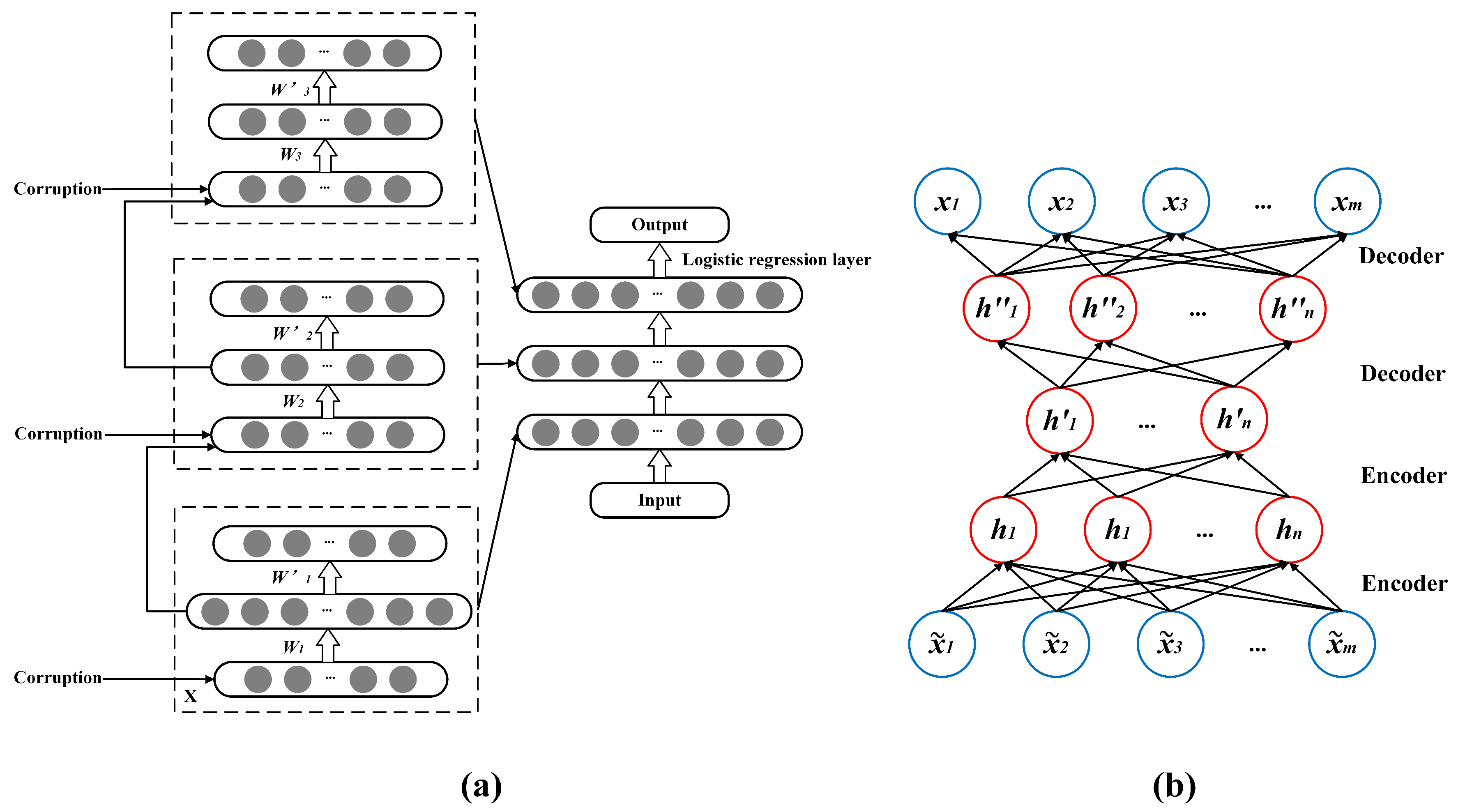
2.2. SDA
- Unsupervised pretrain stage: (1): Train the bottom DAE through the above steps, and an encoder is obtained when the first layer is trained; (2) the feature representation vector is obtained by this encoder on the original input data and regarded as the hidden layer vector, which is used to obtain and train the encoder of the second SDA layer; (3) iterate Steps 1 and 2 for the desired number of SDA layers.
- Supervised fine-tuning stage: When the entire pretraining stage is over, the top layer is the final output layer. With this output as the base layer for logistic regression errors throughout the SDA structure, fine-tuning global parameters are adjusted.
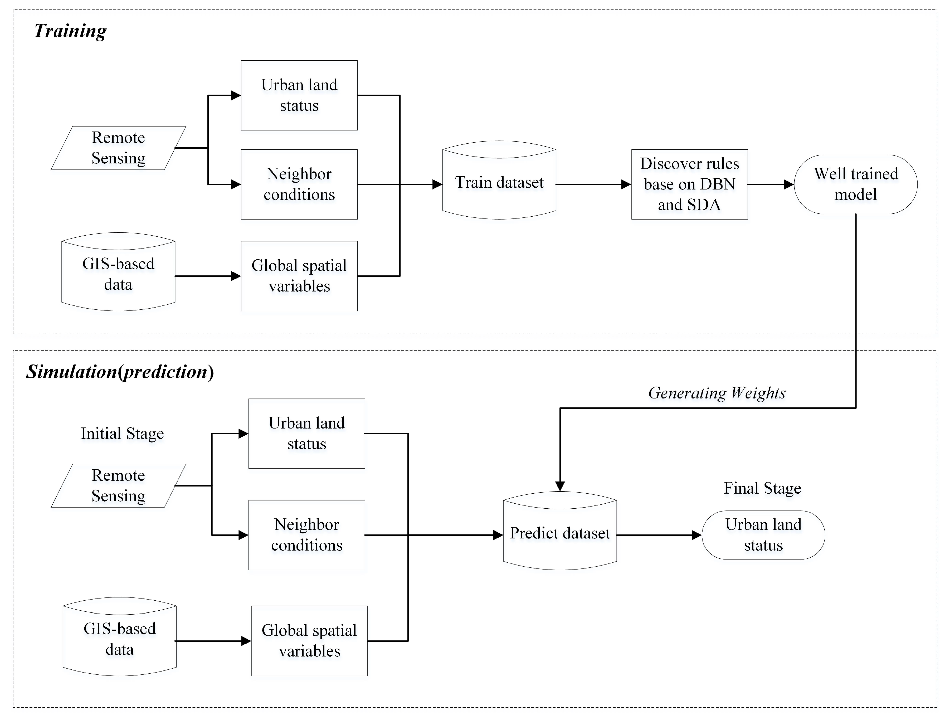
2.3. Proposed Geographical CA Model
2.4. Accuracy Assessment
3. Proposed-Model Implementation
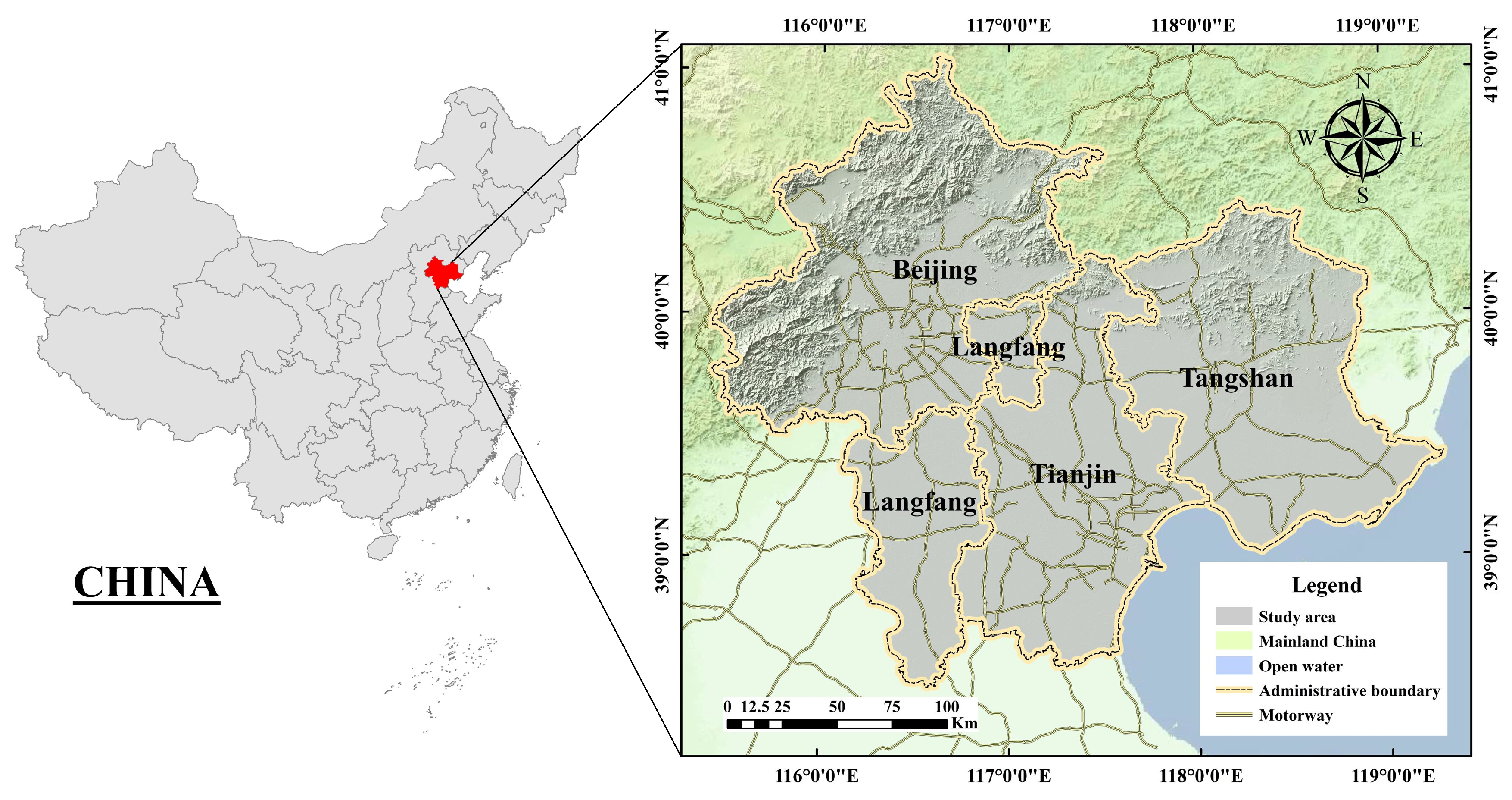
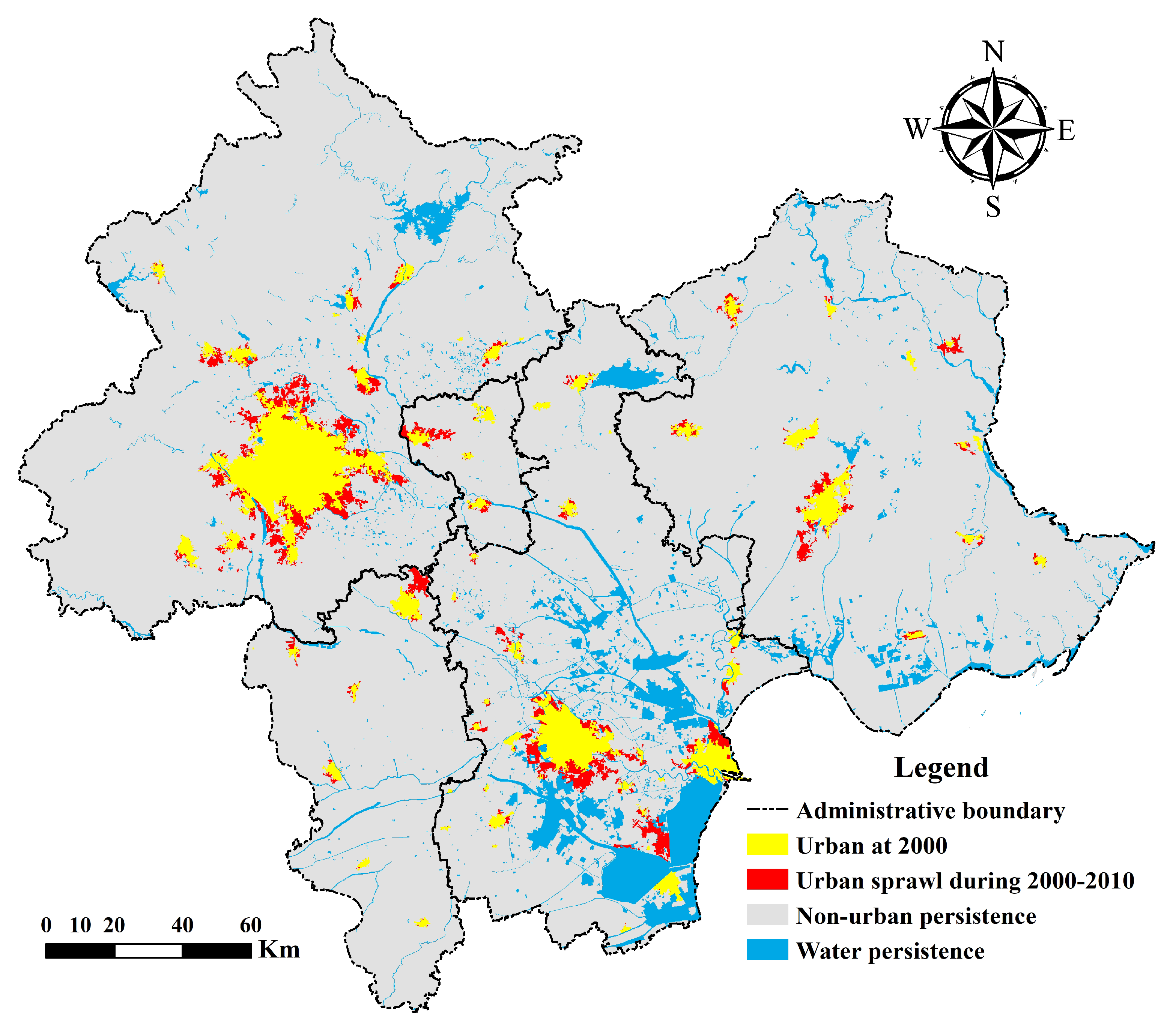
3.1. Study Area
3.2. Data Preprocessing
3.2.1. Land-Use Data
3.2.2. Neighborhood Conditions
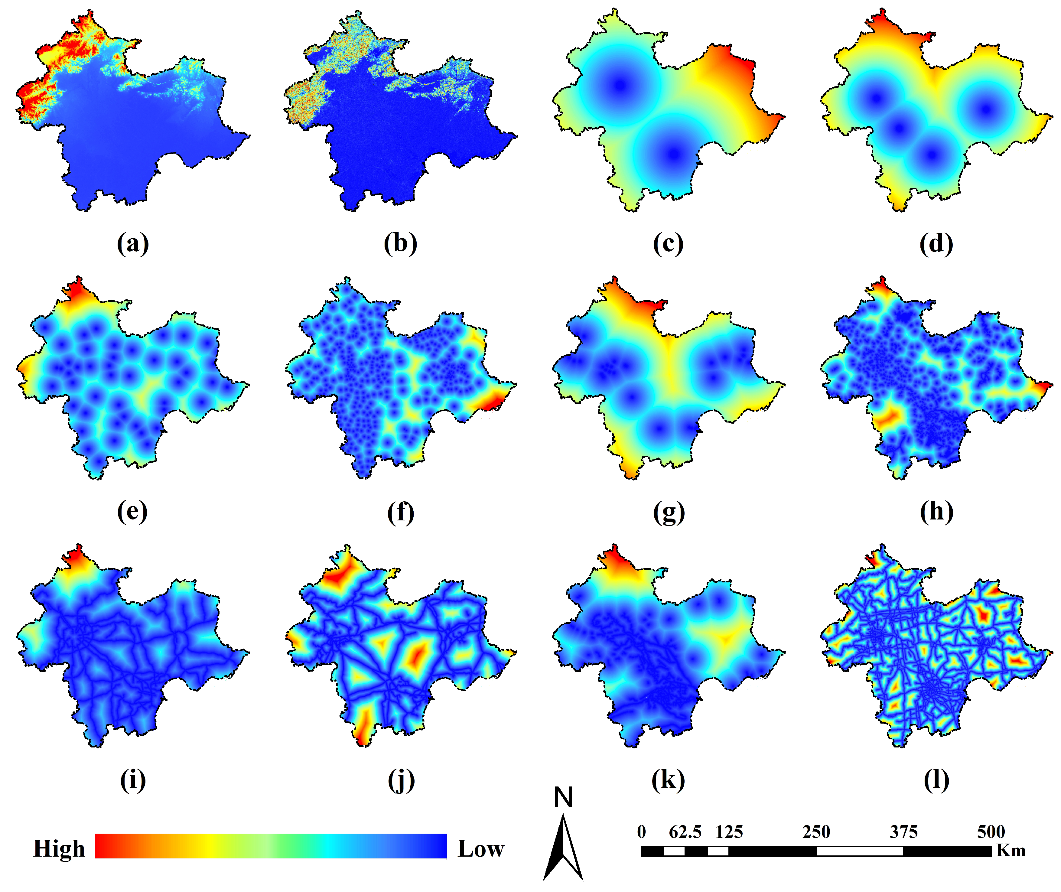
3.2.3. Global Spatial Variables
3.3. Model Design and Computational Environment
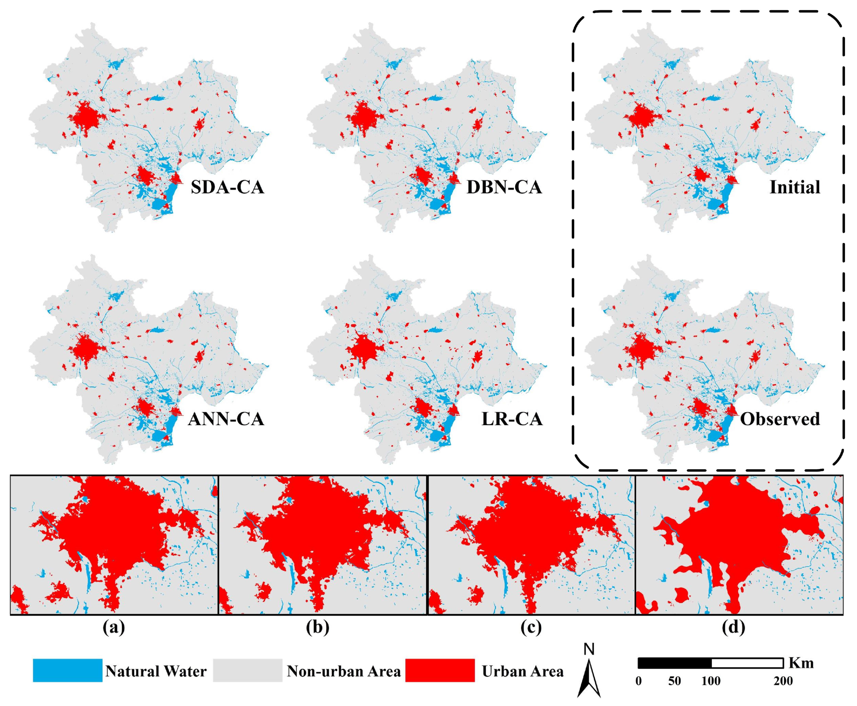
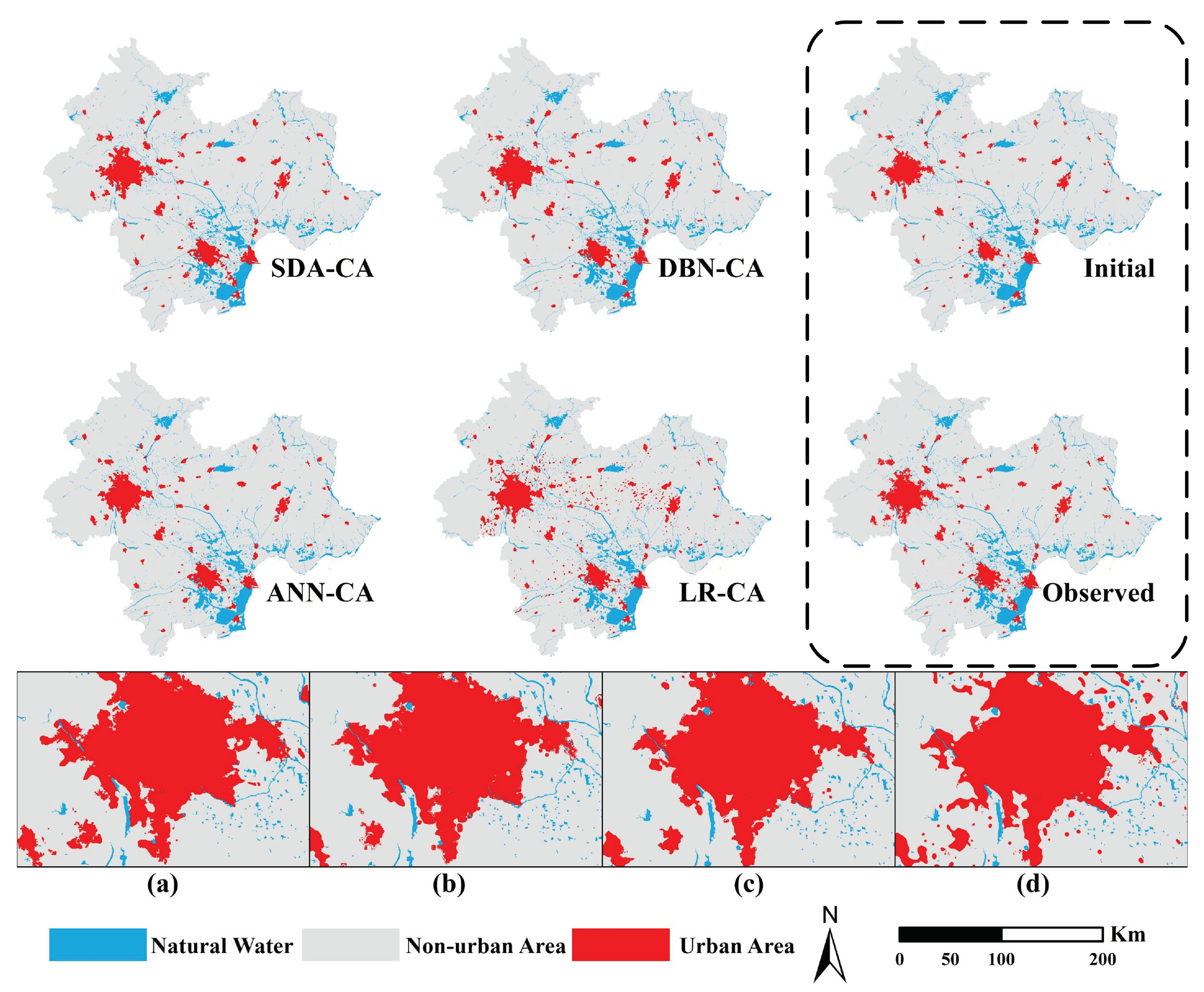
3.4. Simulation Results and Comparisons
4. Discussion and Conclusions
Author Contributions
Funding
Acknowledgments
Conflicts of Interest
References
- Stow, D.A.; Chen, D. Sensitivity of multitemporal NOAA AVHRR data of an urbanizing region to land-use/land-cover changes and misregistration. Remote Sens. Environ. 2002, 80, 297–307. [Google Scholar] [CrossRef]
- Wolfram, S. Universality and complexity in cellular automata. Int. Sympos. Phys. Des. 1984, 10, 1–35. [Google Scholar] [CrossRef]
- Santé, I.; García, A.M.; Miranda, D.; Crecente, R. Cellular automata models for the simulation of real-world urban processes: A review and analysis. Landsc. Urban Plan. 2010, 96, 108–122. [Google Scholar] [CrossRef]
- Liu, X.; Li, X.; Liu, L.; He, J.; Ai, B. A bottom-up approach to discover transition rules of cellular automata using ant intelligence. Int. J. Geogr. Inf. Sci. 2008, 22, 1247–1269. [Google Scholar] [CrossRef]
- Wu, F. SimLand: A prototype to simulate land conversion through the integrated GIS and CA with AHP-derived transition rules. Int. J. Geogr. Inf. Sci. 1998, 12, 63–82. [Google Scholar] [CrossRef]
- Khan, S. Cellular automata-based spatial multi-criteria land suitability simulation for irrigated agriculture. Int. J. Geogr. Inf. Sci. 2011, 25, 131–148. [Google Scholar]
- Lai, T.; Dragićević, S.; Schmidt, M. Integration of multicriteria evaluation and cellular automata methods for landslide simulation modelling. Geomatics Nat. Hazards Risk 2013, 4, 355–375. [Google Scholar] [CrossRef]
- Arsanjani, J.J.; Helbich, M.; Kainz, W.; Boloorani, A.D. Integration of logistic regression, Markov chain and cellular automata models to simulate urban expansion. Int. J. Appl. Earth Obs. Geoinform. 2013, 21, 265–275. [Google Scholar] [CrossRef]
- Almeida, C.M.; Monteiro, A.M.V.; Camara, G.; Soares-Filho, B.S.; Cerqueira, G.C. Modeling The Urban Evolution Of Land Use Transitions Using Cellular Automata And Logistic Regression. In Proceedings of the IEEE International Geoscience & Remote Sensing Symposium, Toulouse, France, 21–25 July 2003. [Google Scholar]
- Chen, Y.; Li, X.; Liu, X.; Ai, B. Modeling urban land-use dynamics in a fast developing city using the modified logistic cellular automaton with a patch-based simulation strategy. Int. J. Geogr. Inf. Sci. 2014, 28, 234–255. [Google Scholar] [CrossRef]
- Li, X.; Yeh, A.G. Neural-network-based cellular automata for simulating multiple land use changes using GIS. Int. J. Geogr. Inf. Sci. 2002, 16, 323–343. [Google Scholar] [CrossRef]
- Huang, W.; Liu, H.; Bai, M. Urban expansion simulation based on constrained Artificial Neural Network cellular automata model. In Proceedings of the International Conference on Geoinformatics, Fairfax, VA, USA, 12–14 August 2009. [Google Scholar]
- Basse, R.M.; Omrani, H.; Charif, O.; Gerber, P.; Bódis, K. Land use changes modelling using advanced methods: Cellular automata and artificial neural networks. The spatial and explicit representation of land cover dynamics at the cross-border region scale. Appl. Geogr. 2014, 53, 160–171. [Google Scholar] [CrossRef]
- Ozturk, D. Urban Growth Simulation of Atakum (Samsun, Turkey) Using Cellular Automata-Markov Chain and Multi-Layer Perceptron-Markov Chain Models. Remote Sens. 2015, 7, 5918–5950. [Google Scholar] [CrossRef]
- Yang, Q.; Li, X.; Shi, X. Cellular automata for simulating land use changes based on support vector machines. Comput. Geosci. 2008, 34, 592–602. [Google Scholar] [CrossRef]
- Rienow, A.; Goetzke, R. Supporting SLEUTH—Enhancing a cellular automaton with support vector machines for urban growth modeling. Comput. Environ. Urban Syst. 2015, 49, 66–81. [Google Scholar] [CrossRef]
- Okwuashi, O.; Nwilo, P.; Mcconchie, J.; Eyo, E. Enhancing a GIS Cellular Automata model of land use change using Support Vector Machine. In Proceedings of the International Conference on Geoinformatics, Fairfax, VA, USA, 12–14 August 2009. [Google Scholar]
- Li, X.; Yeh, A.G. Data mining of cellular automata’s transition rules. Int. J. Geogr. Inf. Sci. 2004, 18, 723–744. [Google Scholar] [CrossRef]
- Florencio Ballestores, Z.Q. An integrated parcel-based land use change model using cellular automata and decision tree. Proc. Int. Acad. Ecol. Environ. Sci. 2012, 2, 53. [Google Scholar]
- Kamusoko, C.; Gamba, J. Simulating Urban Growth Using a Random Forest-Cellular Automata (RF-CA) Model. ISPRS Int. J. Geo-Inf. 2015, 4, 447–470. [Google Scholar] [CrossRef]
- Yao, Y.; Liu, X.; Zhang, D.; Liang, Z.; Zhang, Y. Simulation of Urban Expansion and Farmland Loss in China by Integrating Cellular Automata and Random Forest. arXiv 2017, preprint. arXiv:1705.05651. [Google Scholar]
- Jenerette, G.D.; Wu, J. Analysis and simulation of land-use change in the central Arizona—Phoenix region, USA. Landsc. Ecol. 2001, 16, 611–626. [Google Scholar] [CrossRef]
- García, A.M.; Santé, I.; Boullón, M.; Crecente, R. Calibration of an urban cellular automaton model by using statistical techniques and a genetic algorithm. Application to a small urban settlement of NW Spain. Int. J. Geogr. Inf. Sci. 2013, 27, 1593–1611. [Google Scholar] [CrossRef]
- Xiaoping, L.; Xia, L.; Yeh, A.G.; Jinqiang, H.E.; Jia, T. Discovery of transition rules for geographical cellular automata by using ant colony optimization. Sci. China-Earth Sci. 2007, 50, 1578–1588. [Google Scholar]
- Feng, Y.; Liu, Y.; Tong, X.; Liu, M.; Deng, S. Modeling dynamic urban growth using cellular automata and particle swarm optimization rules. Landsc. Urban Plan. 2011, 102, 188–196. [Google Scholar] [CrossRef]
- Yang, J.; Tang, G.; Cao, M.; Zhu, R. An intelligent method to discover transition rules for cellular automata using bee colony optimisation. Int. J. Geogr. Inf. Sci. 2013, 27, 1849–1864. [Google Scholar] [CrossRef]
- Cao, M.; Tang, G.; Shen, Q.; Wang, Y. A new discovery of transition rules for cellular automata by using cuckoo search algorithm. Int. J. Geogr. Inf. Syst. 2015, 29, 806–824. [Google Scholar] [CrossRef]
- Cao, M.; Bennett, S.J.; Shen, Q.; Xu, R. A bat-inspired approach to define transition rules for a cellular automaton model used to simulate urban expansion. Int. J. Geogr. Inf. Sci. 2016, 30, 1–19. [Google Scholar] [CrossRef]
- He, C.; Zhao, Y.; Tian, J.; Shi, P. Modeling the urban landscape dynamics in a megalopolitan cluster area by incorporating a gravitational field model with cellular automata. Landsc. Urban Plan. 2013, 113, 78–89. [Google Scholar] [CrossRef]
- Bengio, Y.; Courville, A.; Vincent, P. Unsupervised Feature Learning and Deep Learning: A Review and New Perspectives. CoRR 2012, abs/1206.5538. [Google Scholar]
- Najafabadi, M.M.; Villanustre, F.; Khoshgoftaar, T.M.; Seliya, N.; Wald, R.; Muharemagic, E. Deep learning applications and challenges in big data analytics. J. Big Data 2015, 2, 1. [Google Scholar] [CrossRef]
- Vincent, P.; Larochelle, H.; Bengio, Y.; Manzagol, P.A. Extracting and composing robust features with denoising autoencoders. In Proceedings of the International Conference on Machine Learning, Helsinki, Finland, 5–9 July 2008; pp. 1096–1103. [Google Scholar]
- Chen, Y.; Zhao, X.; Jia, X. Spectral–Spatial Classification of Hyperspectral Data Based on Deep Belief Network. IEEE J. Sel. Top. Appl. Earth Obs. Remote Sens. 2015, 8, 2381–2392. [Google Scholar] [CrossRef]
- Budiman, A.; Fanany, M.I.; Basaruddin, C. Stacked Denoising Autoencoder for feature representation learning in pose-based action recognition. In Proceedings of the 2014 IEEE 3rd Global Conference on Consumer Electronics (GCCE), Tokyo, Japan, 7–10 October 2014. [Google Scholar]
- Erhan, D.; Bengio, Y.; Courville, A.C.; Manzagol, P.; Vincent, P.; Bengio, S. Why Does Unsupervised Pre-training Help Deep Learning? J. Mach. Learn. Res. 2010, 11, 625–660. [Google Scholar]
- Vincent, P.; Larochelle, H.; Lajoie, I.; Bengio, Y.; Manzagol, P. Stacked Denoising Autoencoders: Learning Useful Representations in a Deep Network with a Local Denoising Criterion. J. Mach. Learn. Res. 2010, 11, 3371–3408. [Google Scholar]
- Hinton, G.E.; Salakhutdinov, R.R. Reducing the Dimensionality of Data with Neural Networks. Science 2006, 313, 504–507. [Google Scholar] [CrossRef] [PubMed]
- Arsa, D.M.S.; Jati, G.; Mantau, A.J.; Wasito, I. Dimensionality reduction using deep belief network in big data case study: Hyperspectral image classification. In Proceedings of the International Workshop on Big Data & Information Security, Jakarta, Indonesia, 18–19 October 2017. [Google Scholar]
- Zabalza, J.; Ren, J.; Zhao, H.; Zhao, H.; Qing, C.; Yang, Z.; Du, P.; Marshall, S. Corrigendum to ‘Novel segmented stacked autoencoder for effective dimensionality reduction and feature extraction in hyperspectral imaging’ Neurocomputing 185 (2016) 1–10. Neurocomputing 2016, 214, 1062. [Google Scholar] [CrossRef]
- Romeu, P.; Zamora-Martínez, F.; Botella-Rocamora, P.; Pardo, J. Stacked Denoising Auto-Encoders for Short-Term Time Series Forecasting; Springer: Cham, Switzerland, 2015. [Google Scholar]
- Long, W.; Zhang, Z.; Chen, J. Short-Term Electricity Price Forecasting with Stacked Denoising Autoencoders. IEEE Trans. Power Syst. 2017, 32, 2673–2681. [Google Scholar]
- Kuremoto, T.; Kimura, S.; Kobayashi, K.; Obayashi, M. Time series forecasting using a deep belief network with restricted Boltzmann machines. Neurocomputing 2014, 137, 47–56. [Google Scholar] [CrossRef]
- Ahmed, M.; Shill, P.C.; Islam, K.; Mollah, M.A.S.; Akhand, M.A.H. Acoustic modeling using deep belief network for Bangla speech recognition. In Proceedings of the 2015 18th International Conference on Computer and Information Technology (ICCIT), Dhaka, Bangladesh, 21–23 December 2016. [Google Scholar]
- Mohamed, A.R.; Dahl, G.E.; Hinton, G. Acoustic Modeling Using Deep Belief Networks. IEEE Trans. Audio Speech Lang. Process. 2011, 20, 14–22. [Google Scholar] [CrossRef]
- Liu, J.H.; Zheng, W.Q.; Zou, Y.X. A Robust Acoustic Feature Extraction Approach Based on Stacked Denoising Autoencoder. In Proceedings of the IEEE International Conference on Multimedia Big Data, Beijing, China, 20–22 April 2015. [Google Scholar]
- Gu, F.; Khoshelham, K.; Valaee, S.; Shang, J.; Rui, Z. Locomotion Activity Recognition Using Stacked Denoising Autoencoders. IEEE Internet Things J. 2018, 5, 2085–2093. [Google Scholar] [CrossRef]
- Gu, F.; Flórezrevuelta, F.; Monekosso, D.; Remagnino, P. Marginalised Stacked Denoising Autoencoders for Robust Representation of Real-Time Multi-View Action Recognition. Sensors 2015, 15, 17209–17231. [Google Scholar] [CrossRef] [PubMed]
- Wicht, B.; Henneberty, J. Mixed handwritten and printed digit recognition in Sudoku with Convolutional Deep Belief Network. In Proceedings of the 2015 13th International Conference on Document Analysis and Recognition (ICDAR), Tunis, Tunisia, 23–26 August 2015. [Google Scholar]
- He, J.; Li, X.; Yao, Y.; Hong, Y.; Zhang, J. Mining transition rules of cellular automata for simulating urban expansion by using the deep learning techniques. Int. J. Geogr. Inf. Sci. 2018, 32, 2076–2097. [Google Scholar] [CrossRef]
- Zhou, Y.; Zhang, F.; Du, Z.; Ye, X.; Liu, R. Integrating Cellular Automata with the Deep Belief Network for Simulating Urban Growth. Sustainability 2017, 9, 1786. [Google Scholar] [CrossRef]
- Du, G.; Yuan, L.; Shin, K.J.; Managi, S. Enhancement of land-use change modeling using convolutional neural networks and convolutional denoising autoencoders. arXiv 2018, preprint. arXiv:1803.01159. [Google Scholar]
- Testolin, A.; Piccolini, M.; Suweis, S. Deep Learning Systems as Complex Networks. arXiv 2018, preprint. arXiv:1809.10941. [Google Scholar]
- Hinton, G.E. Training Products of Experts by Minimizing Contrastive. Neural Comput. 2002, 14, 1771–1800. [Google Scholar] [CrossRef]
- Qin, M.; Li, Z.; Du, Z. Red tide time series forecasting by combining ARIMA and deep belief network. Knowl.-Based Syst. 2017, 125, 39–52. [Google Scholar] [CrossRef]
- White, R.; Engelen, G. Cellular Automata and Fractal Urban Form: A Cellular Modelling Approach to the Evolution of Urban Land-Use Patterns. Environ. Plan. A 1993, 25, 1175–1199. [Google Scholar] [CrossRef]
- Salapayca, S.; Jankowski, P.; Clarke, K.C.; Kyriakidis, P.C.; Nara, A. A meta-modeling approach for spatio-temporal uncertainty and sensitivity analysis: An application for a cellular automata-based Urban growth and land-use change model. Int. J. Geogr. Inf. Sci. 2018, 32, 637–662. [Google Scholar] [CrossRef]
- Pontius, R.G., Jr.; Walker, R.; Yao-Kumah, R.; Arima, E.; Aldrich, S.; Vergara, M.C.D. Accuracy Assessment for a Simulation Model of Amazonian Deforestation. Ann. Assoc. Am. Geogr. 2010, 97, 677–695. [Google Scholar] [CrossRef]
- Chen, H.; Pontius, R.G., Jr. Diagnostic tools to evaluate a spatial land change projection along a gradient of an explanatory variable. Landsc. Ecol. 2010, 25, 1319–1331. [Google Scholar] [CrossRef]
- Zilinskas, A. Simulation-Based Optimization: Parametric Optimization Techniques and Reinforcement Learning. Interfaces 2003, 35, 535–536. [Google Scholar]


| Spatial Variable | Value Range |
|---|---|
| Urban sprawl in 2000–2010 | Remained nonurban area: 0; converted to urban area: 1; remained urban area: 2 |
| Distance to airport | 0–175,594 m |
| Distance to city administrative center | 0–129,142 m |
| Distance to town administrative center | 0–47,261 m |
| Distance to county administrative center | 0–63,279 m |
| Distance to reservoir | 0–44,457 m |
| Distance to river | 0–88,911 m |
| Distance to railway station | 0–109,976 m |
| Distance to motorway | 0–70,052 m |
| Distance to trunkway | 0–21,979 m |
| Distance to railway | 0–33,278 m |
| Urban cells in neighborhood | 0–48 |
| Land use type | urban area: 1; nonurban area: 0 |
| Elevation | −52–2224 m |
| Slope | 0–69 |
| Description | Symbol | DBN | SDA |
|---|---|---|---|
| Input dimension | n_ins | 11 | 11 |
| Output dimension | n_out | 3 | 3 |
| Intermediate layer size | hidden_layer_sizes | [30, 30, 30] | [30, 30, 30] |
| Number of epochs for pretraining | pre-training_epochs | 300 | 300 |
| Maximal number of iterations of running optimizer | training_epochs | 3000 | 3000 |
| Learning rate used in pretraining | pretrain_lr | 0.01 | 0.001 |
| Learning rate used in fine-tuning stage | finetune_lr | 0.1 | 0.01 |
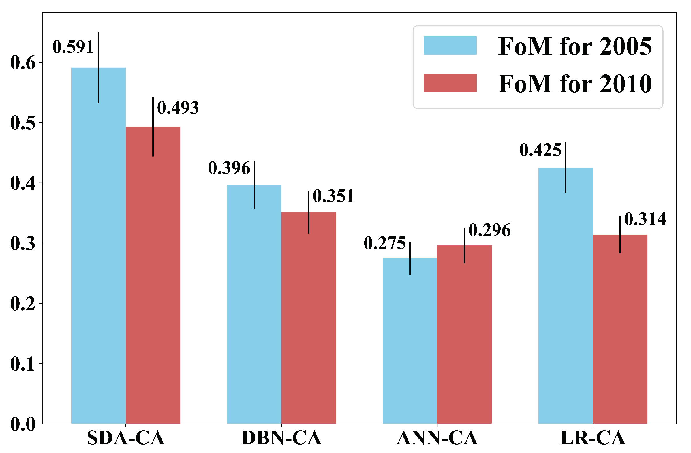
| SDA-CA | DBN-CA | ANN-CA | LR-CA | |
|---|---|---|---|---|
| 2005 | ||||
| Beijing | 0.583 | 0.385 | 0.243 | 0.415 |
| Tianjin | 0.581 | 0.403 | 0.280 | 0.505 |
| Tangshan | 0.579 | 0.367 | 0.320 | 0.315 |
| 2010 | ||||
| Beijing | 0.468 | 0.343 | 0.277 | 0.294 |
| Tianjin | 0.523 | 0.364 | 0.313 | 0.440 |
| Tangshan | 0.432 | 0.332 | 0.299 | 0.199 |
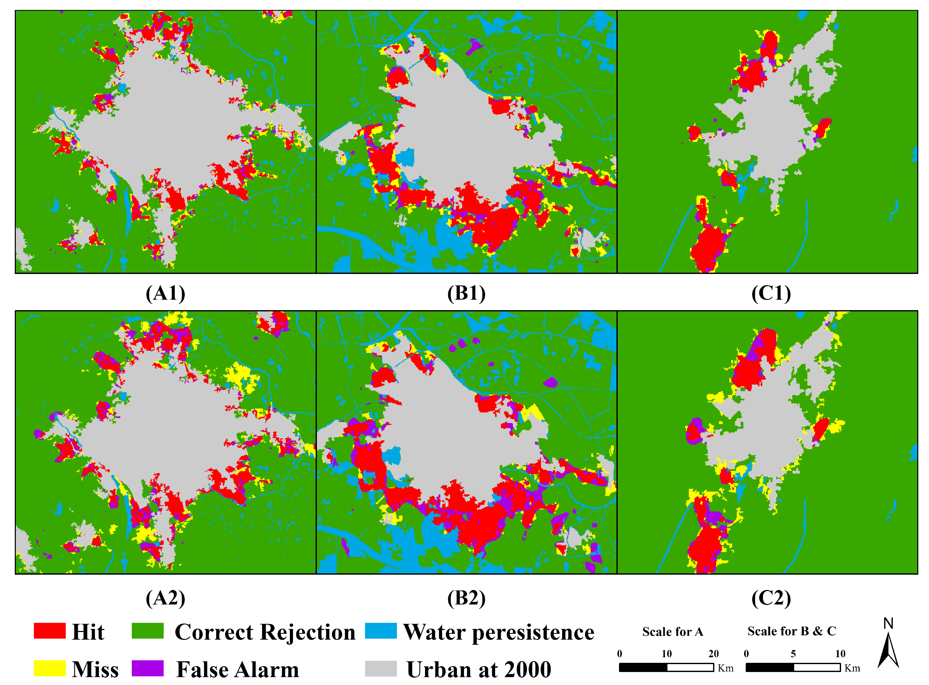
| SDA–CA | DBN–CA | ANN–CA | LR–CA | |
|---|---|---|---|---|
| 2005 | ||||
| Hit | 244528 | 230445 | 219001 | 230811 |
| Miss | 20247 | 34330 | 45774 | 35547 |
| False alarm | 12555 | 16195 | 11364 | 33964 |
| Correcct rejection | 4514091 | 4510451 | 4515282 | 4491099 |
| 2010 | ||||
| Hit | 255148 | 236676 | 231238 | 235346 |
| Miss | 28638 | 47110 | 52548 | 48440 |
| False alarm | 32785 | 36148 | 42303 | 64997 |
| Correcct rejection | 4474850 | 4471487 | 4465332 | 4442638 |
| NP | ED | LSI | AWMPFD | AI | S_i | |
|---|---|---|---|---|---|---|
| 2005 | ||||||
| observed | 142 | 1.019 | 23.889 | 1.175 | 95.539 | - |
| SDA-CA | 179 | 0.855 | 20.385 | 1.159 | 96.166 | |
| DBN-CA | 193 | 0.815 | 19.842 | 1.154 | 96.196 | |
| ANN-CA | 229 | 0.818 | 20.614 | 1.155 | 95.905 | |
| LR-CA | 365 | 0.591 | 13.801 | 1.089 | 97.513 | |
| 2010 | ||||||
| observed | 179 | 1.174 | 26.579 | 1.186 | 95.187 | - |
| SDA-CA | 191 | 0.831 | 18.725 | 1.145 | 96.688 | |
| DBN-CA | 229 | 0.884 | 20.384 | 1.148 | 96.281 | |
| ANN-CA | 215 | 0.635 | 14.613 | 1.122 | 97.390 | |
| LR-CA | 361 | 1.080 | 23.705 | 1.101 | 95.846 |
© 2019 by the authors. Licensee MDPI, Basel, Switzerland. This article is an open access article distributed under the terms and conditions of the Creative Commons Attribution (CC BY) license (http://creativecommons.org/licenses/by/4.0/).
Share and Cite
Ou, C.; Yang, J.; Du, Z.; Zhang, X.; Zhu, D. Integrating Cellular Automata with Unsupervised Deep-Learning Algorithms: A Case Study of Urban-Sprawl Simulation in the Jingjintang Urban Agglomeration, China. Sustainability 2019, 11, 2464. https://doi.org/10.3390/su11092464
Ou C, Yang J, Du Z, Zhang X, Zhu D. Integrating Cellular Automata with Unsupervised Deep-Learning Algorithms: A Case Study of Urban-Sprawl Simulation in the Jingjintang Urban Agglomeration, China. Sustainability. 2019; 11(9):2464. https://doi.org/10.3390/su11092464
Chicago/Turabian StyleOu, Cong, Jianyu Yang, Zhenrong Du, Xin Zhang, and Dehai Zhu. 2019. "Integrating Cellular Automata with Unsupervised Deep-Learning Algorithms: A Case Study of Urban-Sprawl Simulation in the Jingjintang Urban Agglomeration, China" Sustainability 11, no. 9: 2464. https://doi.org/10.3390/su11092464