Article

Understanding the Spatial Structure of Urban Commuting Using Mobile Phone Location Data: A Case Study of Shenzhen, China

1
School of Geography and Tourism, Shaanxi Normal University, Xi’an 710119, China
2
Shaanxi Key Laboratory of Tourism Informatics, Xi’an 710119, China
3
State Key Laboratory of Information Engineering in Surveying, Mapping and Remote Sensing, Wuhan University, Wuhan 430079, China
4
Shenzhen Institutes of Advanced Technology, Chinese Academy of Sciences, 1068 Xueyuan Road, Shenzhen 518005, China
5
College of Urban and Environmental Sciences, Central China Normal University, Wuhan 430079, China
6
School of Architecture and Urban Planning, Huazhong University of Science and Technology, Wuhan 430074, China
*
Author to whom correspondence should be addressed.
Sustainability 2018, 10(5), 1435; https://doi.org/10.3390/su10051435
Submission received: 11 April 2018 / Revised: 2 May 2018 / Accepted: 3 May 2018 / Published: 5 May 2018
(This article belongs to the Section Sustainable Transportation)

Abstract

:
Understanding commuting patterns has been a classic research topic in the fields of geography, transportation and urban planning, and it is significant for handling the increasingly serious urban traffic congestion and air pollution and their impacts on the quality of life. Traditional studies have used travel survey data to investigate commuting from the aspects of commuting mode, efficiency and influence factors. Due to the limited sample size of these data, it is difficult to examine the large-scale commuting patterns of urban citizens, especially when exploring the spatial structure of commuting. This study attempts to understand the spatial structure characteristics generated by human commutes to work by using massive mobile phone datasets. A three-step workflow was proposed to accomplish this goal, which includes extracting the home and work locations of phone users, detecting the communities from the commuting network, and identifying the commuting convergence and divergence areas for each community. A case study of Shenzhen, China was implemented to determine the commuting structure. We found that there are thirteen communities detected from the commuting network and that some of the communities are in accordance with urban planning; moreover, spatial polycentric polygons exist in each community. These findings can be referenced by urban planners or policy-makers to optimize the spatial layout of the urban functional zones.

Graphical Abstract

1. Introduction

Investigating commuting patterns is a long-term and crucial research topic in the fields of transport, geography and urban studies. Commuting behavior is considered an individual movement between a residence and a workplace, which is an essential part of urban life [1,2]. Currently, with the rapid urban expansion and the substantial growth of private cars, people could choose a workplace and a residence according to their preference and income level, which leads to a spatial mismatch of commuting flow and has become one of the primary reasons for urban traffic problems and unhappiness [3]. Therefore, understanding the characteristics of urban commuting plays an important role in alleviating urban traffic congestion [4,5], reducing urban air pollution [6,7] and improving quality of life [2,8].
Traditional techniques for examining the characteristics of commuting depend on the household travel survey dataset, which includes individual detailed socio-demographic properties. Thus, this dataset could be utilized for investigating the influence factors of commuting patterns, such as income level, gender, ethnicity, occupation, and construction environment [9,10,11,12], studying the spatial relationship of workplace–residence location [13,14] or examining the relationship between urban form, land use and commuting [15,16]. However, the collection of this dataset is costly, strenuous and not easily updated in a timely manner; moreover, the limitation of sample size makes it difficult to provide comprehensive evidence of human mobility, especially in understanding the spatial structure characteristics of large-scale urban commuting [17].
Fortunately, recent information and communication technologies (ICTs) change this situation; the widespread use of location-aware devices makes it possible to collect large-scale human spatiotemporal movement trajectory datasets such as mobile phone data, floating car data and smart card data [18,19,20,21,22,23]. These datasets have been widely used to understand the law of urban human mobility and urban structure from the perspective of space and time, such as exploring human convergence and divergence patterns [24], measuring human activity space [25], identifying human spatial interaction communities [26], detecting human mobility hotspots [27], inferring urban land use [28,29,30,31], and quantifying urban dynamic accessibility [32]. For commuting, previous studies have utilized the large geo-tagged datasets to investigate commuting patterns [23,33,34], origin–destination trips [35], commuting efficiency [36] and workplace–residence location relationships [37,38,39]. However, very little work exploits the advantage of the large datasets to understand the urban spatial structure characteristics projected from the commuting patterns. In fact, the relationship between commuting patterns and urban structure has been long examined by geographers using traditional data [1,40,41].
In this paper, we aim to reveal the characteristics of urban spatial structure (such as commuting communities and a polycentric structure) concealed in the massive commuting trips derived from massive mobile phone location data, mainly referring to commuting communities (tightly commuting connected areas) and spatially significant areas of commuting activities. To accomplish this, a three-step workflow was developed by combining complexity network and spatial statistical analysis. First, home and work locations were extracted from human space-time trajectories; then, commuting communities were detected from a spatially directed and weighted network that was constructed based on home-work flows; and finally, we used a spatial statistical method to identify commuting convergence and divergence areas for each community. The commuting convergence areas represent areas that the commuting inflow are larger than the outflow, on the contrary, there are commuting divergence areas. A pilot study of Shenzhen, China has been implemented to disclose the spatial polycentric structure implied in the commuting network.

2. Study Area and Dataset

The study area of this research is Shenzhen, which is located in southern China and neighbors Hong Kong. Since implementing the policy of reform and opening up, Shenzhen was set as the first special economic zone and has undergone rapid economic development over the past three decades. Currently, it has become a famous metropolis around the world and has a population of more than 15 million, which is the highest population density among Chinese cities [42].
The mobile phone location data used in this study were collected by a major mobile phone company, which accounts for approximately 75% of the entire mobile phone market in Shenzhen. It covers one workday’s traces of 16 million mobile phone users. Different from call detail records (CDRs), which record individual location only when communication activities (such as phone calls or text messages) occur, this dataset was originally generated for troubleshooting by mobile operators, and the operator actively recorded the mobile phone location with a regular interval approaching one hour. Each record contains the user ID, recording time, and longitude and latitude of the cell phone tower used (Table 1). Note that the dataset has been processed for privacy protection before it was usable for research. In total, more than 5900 cell phone towers are extracted from the dataset, Figure 1 shows the spatial kernel density of the cell phone towers. This study used the voronoi polygons produced based on the locations of the cell phone towers to denote the service areas. For each voronoi polygon, the points in the polygon are closer to the corresponding cell phone tower than any other [43]. Note that the islands in the left bottom are not considered in the following analysis.
In this study, we selected these mobile subscribers that keep recording in every time window from the original dataset (Table 1). There are some subscribers missing records in some time windows due to the power off of phones or leaving the city, so it is difficult to identify meaningful places such as home and work locations for these users. Finally, there are approximately 6.5 million subscribers who have location records in every time window, and we denoted this selected dataset as D 1 , which is used for this study.

3. Methodology

In this section, a three-step workflow was implemented to uncover the spatial structure of commuting, which includes the estimation of home and work locations, the identification of commuting communities and the detection of the spatially significant commuting convergent and divergent areas for each community.

3.1. Extracting the Home and Work Location

For a single cellphone user in dataset D 1 , the space-time trajectory can be generated by linking the location records according to the order of the updated time, which can be represented as follows:
T r = { p 1 ( x 1 , y 1 , t 1 ) , , p i ( x i , y i , t i ) , , p n ( x n , y n , t n ) } ,
where x i , y i represent the location coordinate of the corresponding cellphone tower (signal tower for connecting with mobile phones) and t i represents the updated time of the point p i .
There are some studies that have developed methods modeling home and work locations using mobile phone data or smart card data [25,37,44]. One of the main procedures is extracting stop locations from the trajectory and analyzing the duration of the stop location during the daytime and nighttime. In this study, the method proposed by Xu et al. (2014) is employed to infer individual home and work locations [45]. Let T k denote the duration of stay for the user at cellphone tower k ; if the duration of stay is more than four hours ( T k 4 ) between 00:00 and 06:00, then the cellphone tower k is considered the user’s home location L h ; if the duration of stay is more than six hours ( T k 6 ) between 09:00 and 18:00, then the cellphone tower k is considered as the user’s work location L w . Based on this rule, the corresponding cellphone towers of home and work locations can be extracted from individual space-time trajectories.

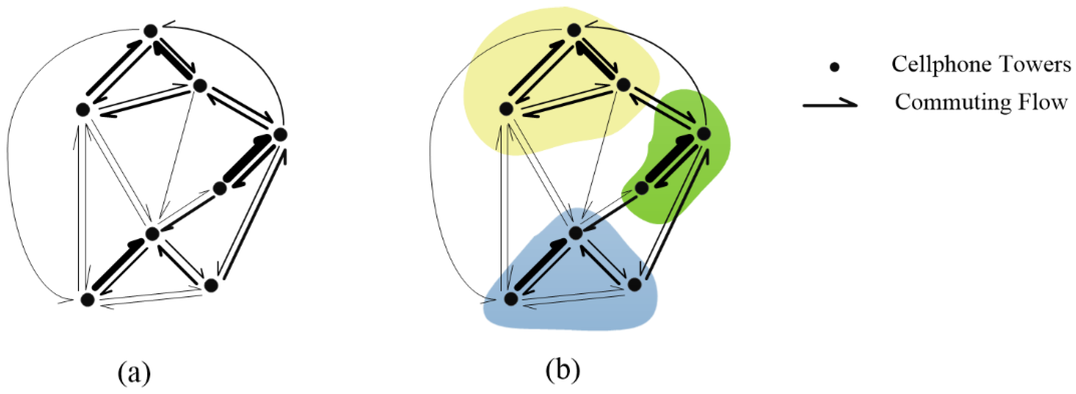
3.2. Detecting the Commuting Communities

In this section, a directed and weighted commuting network was constructed based on identified home and work locations, and communities were detected based on the constructed network.
For each cellphone user whose home and work locations have both been identified, if the home and work locations are not identical ( L h L w ), then a commuting flow can be generated from the home location to the work location. Then, we calculated the total commuting flows for each pair of cellphone towers, and a directed and weighted commuting network G = ( V , E ) can be established among the cellphone towers (Figure 2a). The node V i of the network corresponds to the cellphone tower i , the edge E i j of the network represents the commute from cellphone tower i to cellphone tower j , and the weight of w i j is the number of people commuting from cellphone tower i to cellphone tower j .
Based the constructed directed and weighted commuting network G , we can calculate the sum of the inflow, outflow and net flow for each node V i as follows:
I n i = j = 1 n w j i ,
O u t i = j = 1 n w i j ,
N e t i = I n i O u t i ,
where w i j represents the weight of edge E i j and n indicates the number of total nodes. As described in [24,46], the net flow could represent the difference between the commuting inflow and outflow of a place, and it can be used to indicate the state of human convergence or divergence of a place. Thus, the net flow is employed to identify the commuting convergence and divergence areas in the next section.
In the field of complex networks, a community is constituted by some tightly connected nodes, so the objective of community detection is partitioning the whole network into several densely connected sub networks (Figure 2b). Therefore, the commuting communities would include the tightly connected residential and industrial areas. Recently, the community detection algorithms have been introduced into human mobility studies to determine the spatial interaction of cohesive communities [26,47,48]. There are many community detection algorithms such as Walktrap [49], modularity maximization [50], Infomap [51], etc. Fortunato (2010) compared the performance of 12 different community detection algorithms and found that Infomap shows better performance in detecting weighted and directed networks [52]. This algorithm employs a two-level coding mechanism and finds the optimal community partition by minimizing the expected length of a random walk. A detailed description of the method can be found in [51]. In this study, we executed Infomap by using the igraph package of R [53].

3.3. Identifying Commuting Convergence and Divergence Areas for Each Community

In spatial statistics, the Getis–Ord Gi* index has been frequently used to identify statistically significant spatial clusters of hot spots and cold spots, which has been widely used in geographical analysis [54,55,56]. By calculating the Getis–Ord Gi* index, the method generates a z-score and a p-value for each feature and then finds these features with high (low) values that are also surrounded by other features with high (low) values. In this study, we utilized the net flow N e t i of cellphone tower i as the attribute value to input the method. Therefore, the identified hot spots are these areas where the commuting inflow is larger than the outflow and are denoted as commuting convergence areas in this study. Inversely, cold spots are the areas where the commuting outflow is larger than the inflow and are denoted as commuting divergence areas. It is apparent that these commuting convergence and divergence areas are urban workplace and residence-concentrated areas, respectively.
The hot spot analysis (Getis–Ord Gi*) was executed by using the spatial statistic toolbox embedded in ESRI ArcGIS 10.2 Desktop. We applied this tool to identify commuting convergence or divergence areas for each detected community. The distance band is based on the average neighbor distance among the cellphone towers in the community. The tool creates a new field Gi_Bin for each feature to reflect the statistical significance with a 99%, 95% and 90% confidence level (Figure 3b). We labeled the identified hot and cold polygons at or above a 90% confidence level as “Convergence” and “Divergence”. Based on this label, we combine these adjacent features with the same label into a single polygon (Figure 3c). Hence, we can identify commuting convergence and divergence areas for the detected communities.

4. Results and Discussion

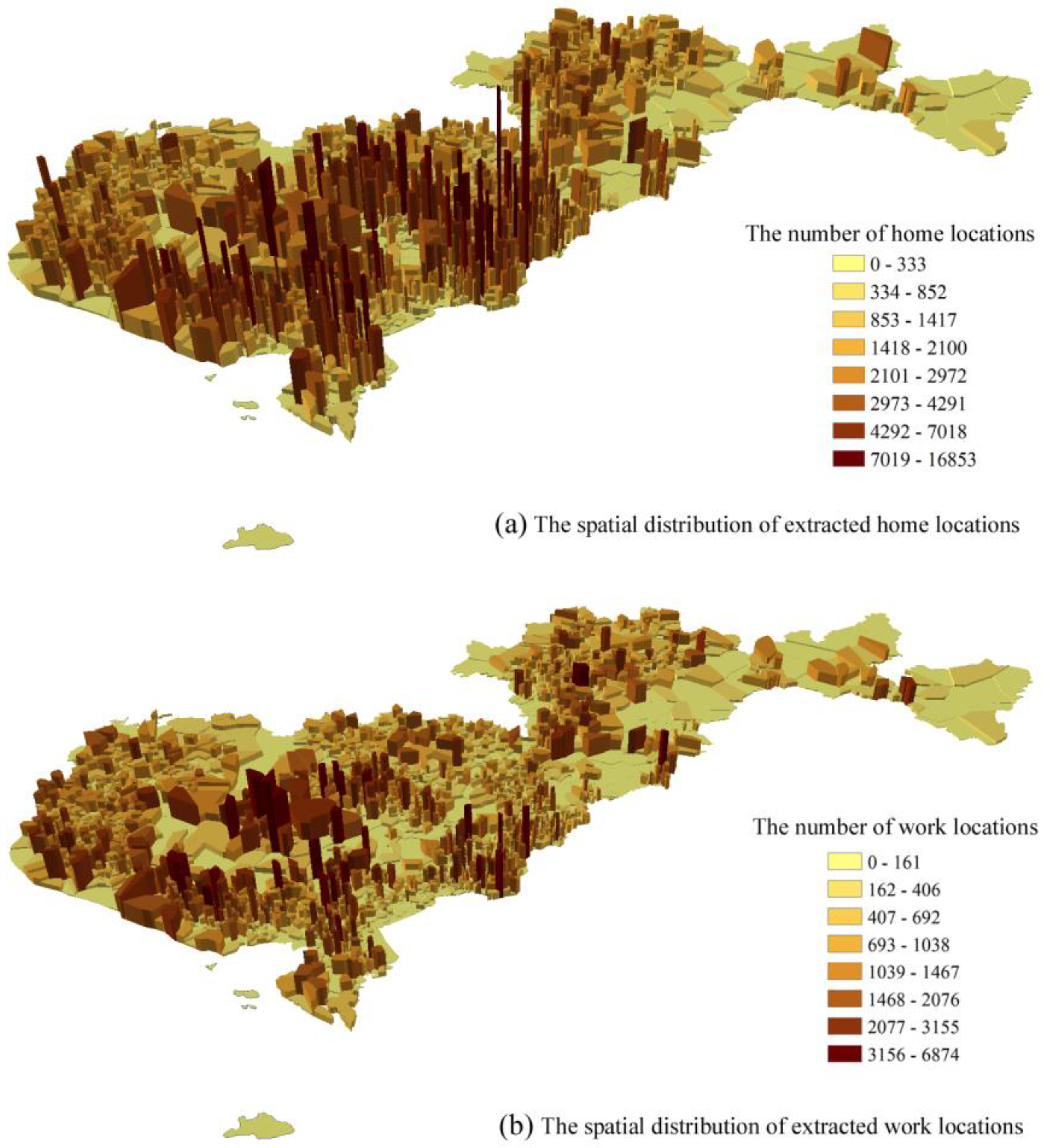
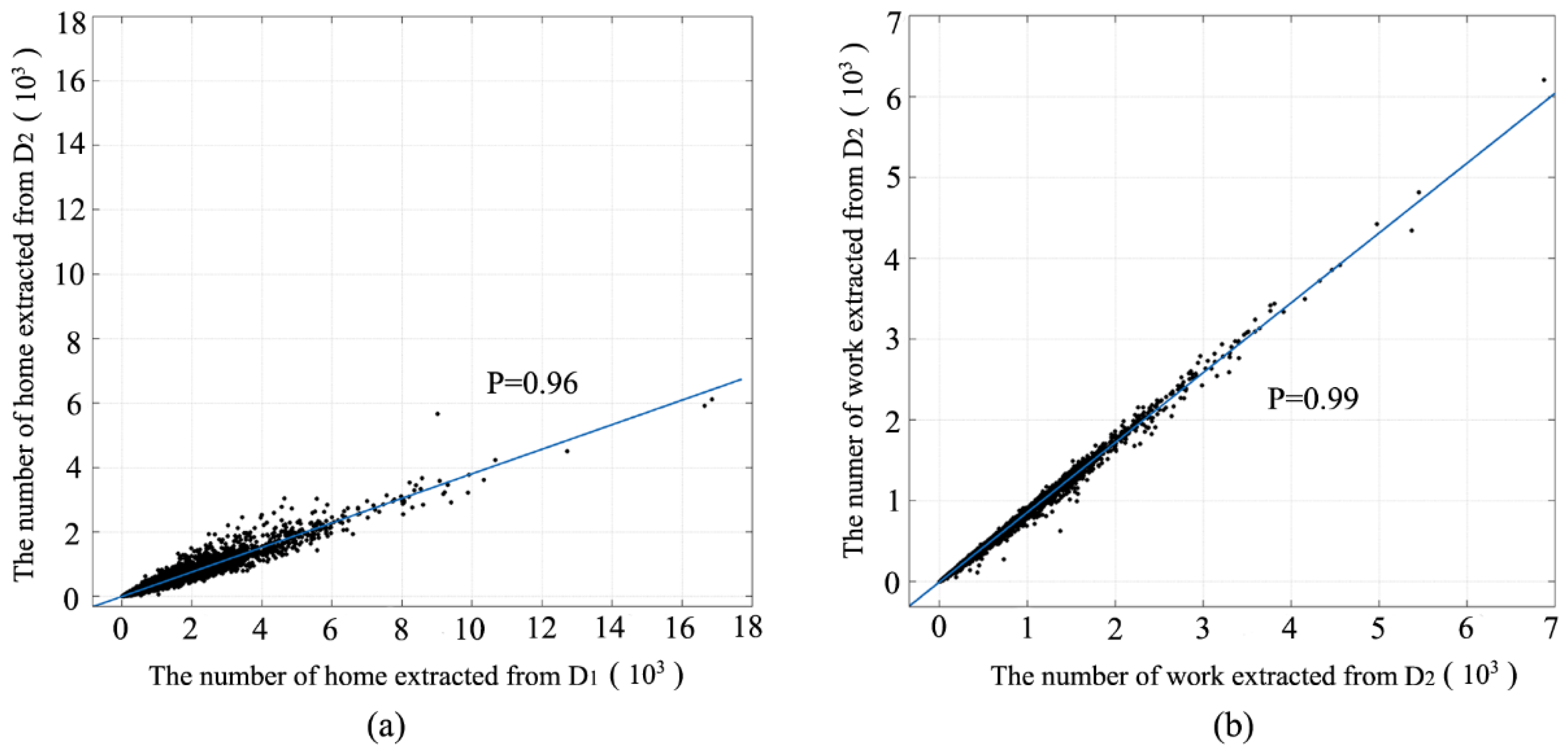
4.1. Extraction of Home and Work Locations

Based on the rule, we extracted home and work locations for every cellphone user in the dataset D 1 . There are more than 5.2 million cellphone users (81.5%) with home locations extracted and more than 2.4 million users (37.6%) with work locations extracted. Figure 4 shows the spatial distribution of the extracted home and work locations for each Voronoi polygon. By comparing these with the travel survey data, Xu et al. (2014) have verified that it is feasible to estimate the workplace–residence distribution using the dataset of this study, based on the urban street blocks, they found that the Spearman’s correlation coefficient for home and work are 0.946 and 0.902 respectively between this mobile phone data and national census data, in addition, by using the shortest path between extracted workplace and residence as commuting distance, the average commuting distance is 5.53 km, which is in line with the traffic survey data (5.40 km) [45].
In dataset D 1 , there are more than 2.1 million cellphone users (32.5%) with both home and work locations extracted; we denoted these users as D 2 , and these users are used to construct the commuting network in the following section. To analyze the representativeness of these users, we compared the spatial distribution of home and work extracted from dataset D 2 with that extracted from dataset D 1 based on cellphone towers. As shown in Figure 5, it can be seen that there is a remarkably linear relationship between D 1 and D 2 for both home and work locations. We calculated the Spearman’s correlation coefficient for the two datasets, and the coefficients of home and work are 0.96 and 0.99, respectively, which demonstrated that dataset D 2 with both home and work locations extracted could be used to explore the spatial characteristic of urban commuting.
Figure 6a shows the distribution of the commuting distance in Shenzhen; note that the distance is calculated by the Euclidean distance based on the corresponding cellphone tower of the home and work location. It is obvious that the number of commuters decreases with the increase in distance, which exhibits a heavy tail distribution. In other words, the majority of people have a short commuting distance (more than 82% of people commute less than five kilometers), while only a few people chose a workplace that has a long commuting distance. Previous studies have found that human mobility follows scaling laws [57], so we utilized a power law p d β to fit this distance decay effect, where p represents the probability of people at commuting distance d and β is the distance decay friction coefficient. Figure 6b plots the log–log distribution of the commuting distance. The distribution can be fitted by a power law function and the friction coefficient β is 1.602, which is consistent with the distance decay law of intra-urban human mobility studied by [58].

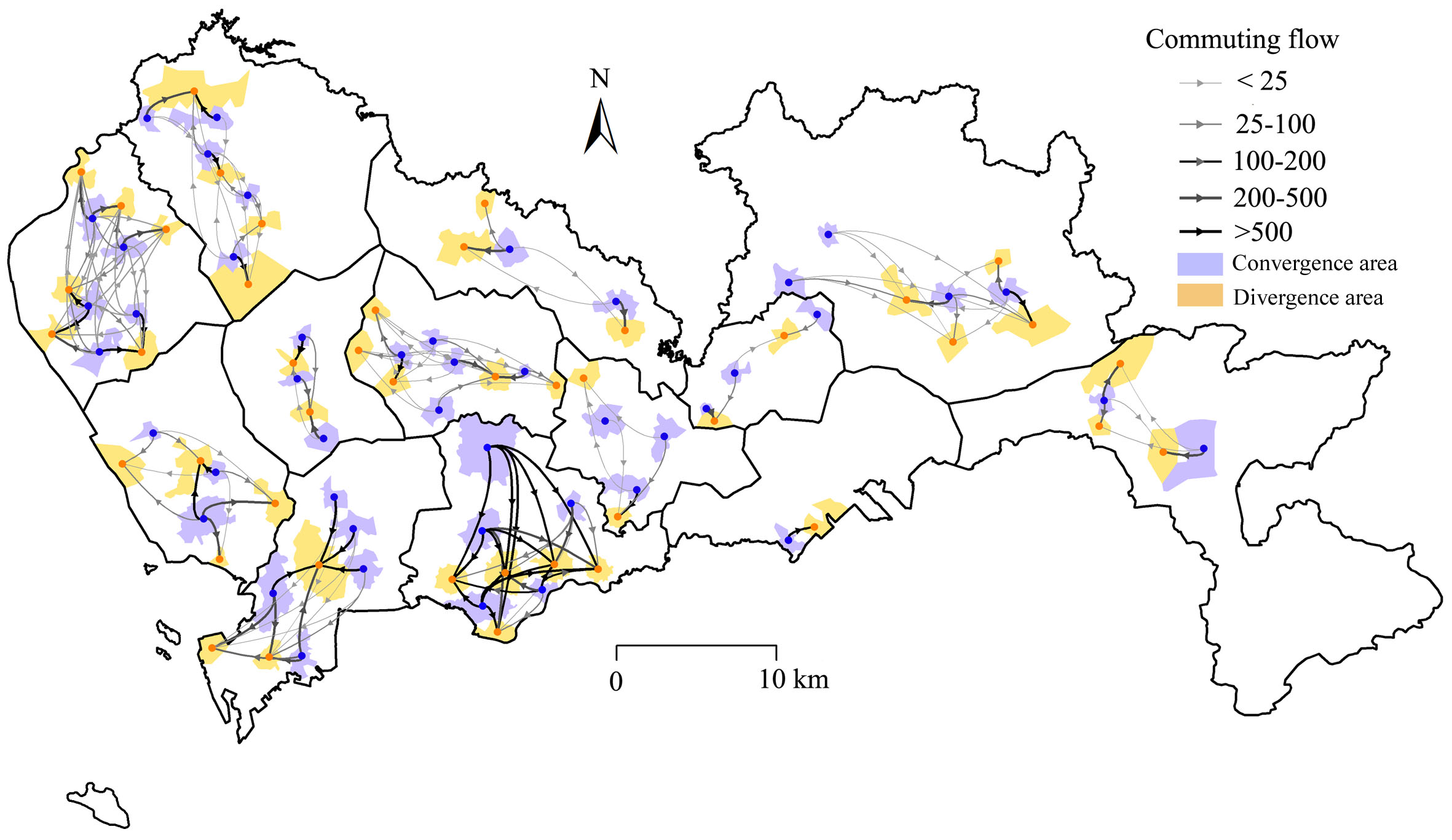
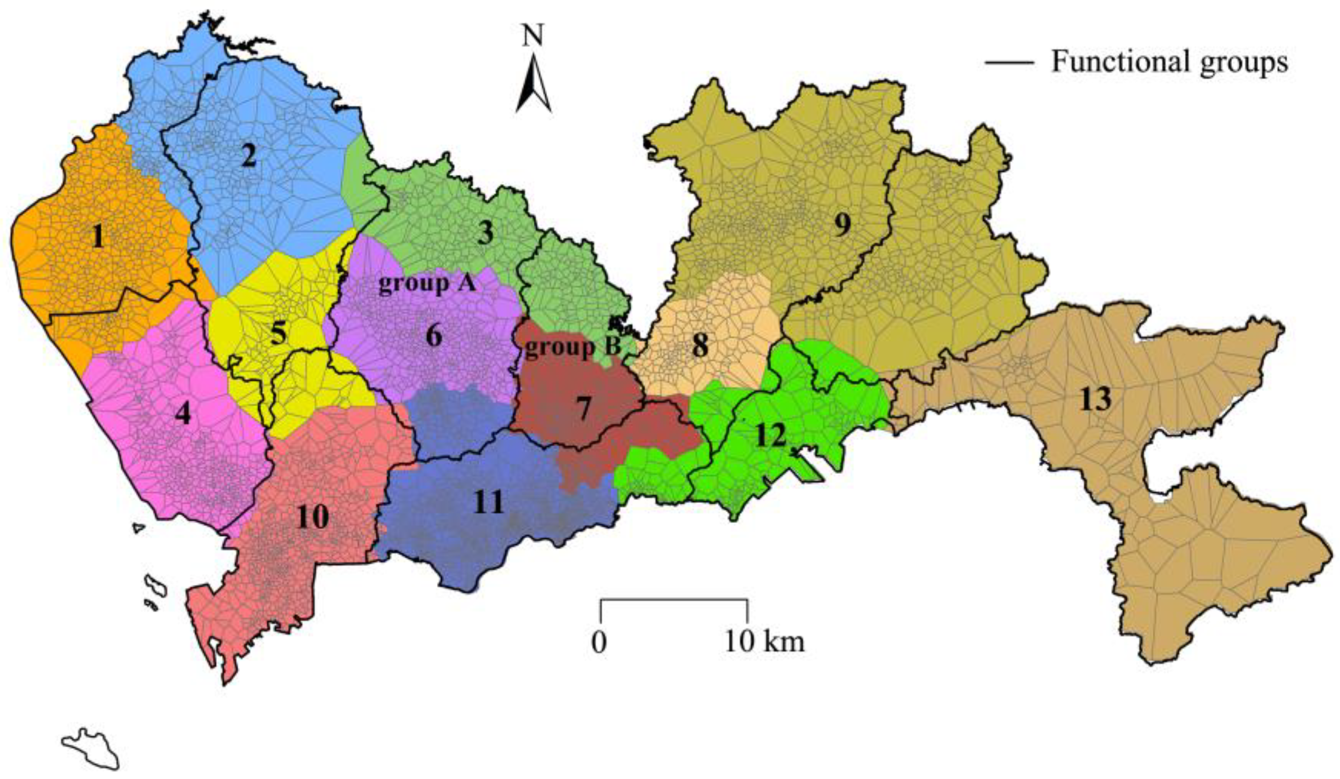
4.2. The Communities Detected Based on Commuting Flows

Based on the constructed directed and weighted commuting network, we first calculated the inflow and outflow of each cellphone tower according to Equations (2) and (3). Figure 7 shows the statistical distribution of inflow and outflow. It is apparent that both inflow and outflow represent a long tail distribution, where 93.8% and 93.6% of cellphone towers are less than 500, and only a few towers have extremely large inflow or outflow values, which indicates that only a few areas in the city might be highly concentrated workplace or residential areas in the city.
Figure 8 illustrates thirteen communities detected from the commuting network. We can see that the spatially adjacent Voronoi polygons were identified as a community, which indicates that the closer the polygons are, the higher the commuting flow is. That is, commuting follows a distance decay law. The number of people commuting among the communities accounts for only approximately six percent of dataset D 2 . For each community, we calculated the total number of people ( N ) who are living in the community, and the percentage of people who work in this community ( P 1 ) and work in other communities ( P 2 ). As shown in Table 2, for each community, there are approximately 90% residents commuting within the community, and only a few residents need to leave the community for work. In other words, the workplace–residence location relationship in these detected communities show an extremely high balance, which indicates that there is a polycentric spatial structure in Shenzhen.
To promote Shenzhen’s industrial intensive development and improve the efficiency of land use, the urban government proposed the planning policy of functional group partitioning. According to the comprehensive urban planning of Shenzhen, the whole city is partitioned into eleven functional groups, which are delineated by the black line in Figure 8. We can see that there are similar partitions between the detected communities and the functional groups of the planning process in the southern part of Shenzhen, while large inconsistencies occur in the northern part of the city (such as communities 4, 10, 11, 12, and 13). One possible explanation is attributed to the economic development disparity of the southern and northern parts. In Shenzhen, the southern part has experienced rapid development in the past few decades, especially for communities 10 and 11, which have become the center of the city, forming mature land use structures in these areas. The main purpose of planning functional groups is to drive the development of the north by adjusting the spatial structure to strengthen the connection between the south and the north such as in functional groups A and B (Figure 8). However, the detected spatial interaction structure reveals that the east–west connection is stronger than the south–north connection in the northern part of the city, which can be demonstrated by communities 3, 6 and 7. In the planning process, the western part of community 3 should show a strong connection with community 6 to form functional group A, while the eastern part should tightly interact with community 7 to generate functional group B, yet the two parts show stronger commuting flow to form community 3. These results can be referenced by urban administrators to optimize the previous planning or to reasonably adjust the spatial structure of the urban industry, especially in the northern part of the city.

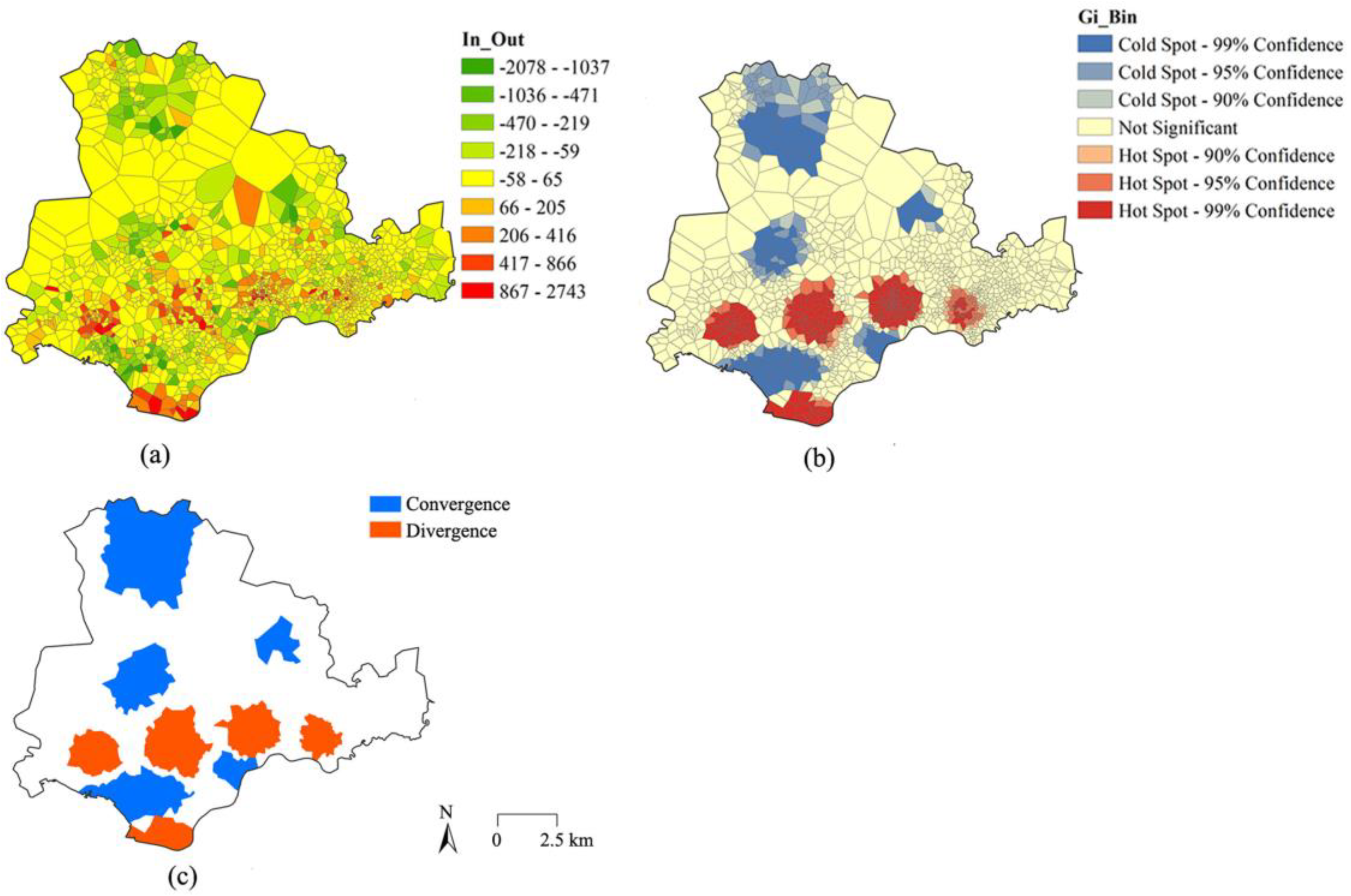
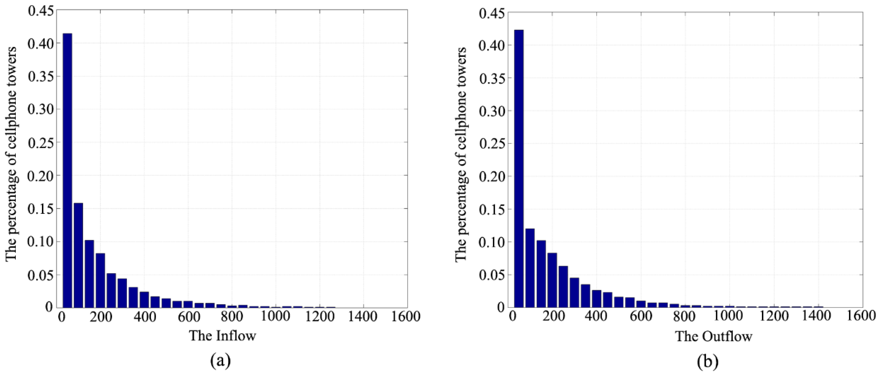
4.3. The Commuting Convergent and Divergent Areas for Each Community

The method described in Section 3.3 was utilized to identify the commuting convergence and divergence areas; note that we applied the method to each community. On the one hand, the population density of the southern part is larger than that of the northern part of Shenzhen; the hot and cold areas might only be detected in the southern part if we applied the Getis–Ord Gi index to the whole city, so we applied the method to each community to relieve the influence of the imbalanced spatial distribution of the population. On the other hand, it allowed us to observe the spatial structure of the workplace–residence locations within each community. We identify a total of 90 significant areas of commuting activity, including 44 commuting convergence areas and 46 commuting divergence areas (Figure 9). By overlapping these areas on the urban functional zones, it can be seen that the commuting convergence areas mainly cover the urban industrial zones and central commercial zones, while the commuting divergence areas are mainly located in the urban residential zones. Therefore, it is known that these areas are the concentrated workplace and residential areas in each community.
To further examine the spatial interaction between commuting divergence areas and commuting convergence areas in each community, we utilized the Bezier curve to visualize the spatial flow from commuting divergence areas to convergence areas for each community (Figure 10). Overall, it can be seen that the commuting flow of the southern part (especially in communities 10 and 11) is larger than that of the northern part, which is due to the spatial distribution of the population in Shenzhen. In addition, we can also see the spatial interaction strength among these commuting areas in Figure 10; we found that most of the commuting divergence areas in the northern part provide workers primarily for one adjacent commuting convergence area. Therefore, this indicates that if two residents live in the same commuting divergence area, they are more likely to work in the same nearby commuting convergence area, which may be caused by two main factors: commuting distance and the number of jobs in the commuting convergence area.
Based on the above analysis, it can be summarized that even for a single detected community, it is also spatially polycentric, which includes several identified commuting convergence and divergence areas. Moreover, from the perspective of spatial interactions, there are pairing phenomena between commuting convergence and divergence areas in the northern part of Shenzhen; that is, the people living in one commuting divergence area mainly flow into one nearby commuting convergence area. This knowledge not only reveals the spatial structure of areas with high traveling activities during the commuting time for each community but also gives an insight into the spatial relationship among these significant commuting activity areas. As a consequence, these findings are helpful for the urban government to make some reasonable policies to benefit the lives of residents in the city. For example, urban planners could reallocate the land use to further optimize the workplace–residence location balance within each community, traffic managers could make some targeted adjustments to the traffic facilities between closely connected commuting activity areas to improve the efficiency of commuting.

5. Conclusions

The development of information and communication technologies (ICTs) not only changes our way of life but also introduces massive human tracking geo-tagged datasets, which provide a great opportunity for studying urban human mobility patterns and spatial structures. This study focused on understanding the spatial structure of urban commuting trips by using mobile phone location data. By combining complex network and spatial statistical analysis methods, we proposed a workflow to identify communities and significant spatial cluster areas formed by commuting flows from home to work.
A case study of Shenzhen, China was implemented. The results show that there is a polycentric spatial structure in Shenzhen, and thirteen communities are detected from the directed and weighted commuting network. We found that there are some inconsistencies between the detected communities and the urban planning function groups, especially in the northern part of Shenzhen, which may be caused by the economic development disparity between the southern and northern parts of the city. For each community, we identified the significant commuting convergence and divergence areas; it can be seen that a polycentric structure occurred even for a single community, and most of the commuting divergence areas provide workers primarily for one adjacent commuting convergence area. These empirical findings give an insight into the spatial structure of urban commuting patterns, which can be referenced by urban planners or policy-makers to optimize the spatial layout of the urban functional zones.
One main limitation of this work is that only one workday’s data is accessible. The method could be improved and the research results could be more reliable if there were weekly data. However, it can be seen that the proposed workflow could identify spatial structure of urban commuting effectively. It can be utilized for monitoring dynamic change of urban commuting when the mobile phone data is potentially widely accessed in the future, which contributes to identifying the change of urban spatial structure so that the departments could adjust the policies in a timely manner.

Author Contributions

This research was mainly conceived and designed by X.Y., Z.F. and L.Y.; X.Y., Y.Z. performed the experiments and wrote the manuscript; S.L., J.L. processed and analyzed the dataset; all authors reviewed the manuscript.

Acknowledgments

This study was jointly supported by National key R & D plan (2017YFC1405302, 2017YFB0503802), National Natural Science Foundation of China (Grants 41771473, 41231171, 41571135, 41771441), and the Fundamental Research Funds for the Central Universities (Grants GK201803049, 2042017kf0235), and China Postdoctoral Science Foundation (No. 2017M623112, 2018M632860).

Conflicts of Interest

The authors declare no conflict of interest.

References

  1. Sohn, J. Are commuting patterns a good indicator of urban spatial structure? J. Transp. Geogr. 2005, 13, 306–317. [Google Scholar] [CrossRef]
  2. Ta, N.; Chai, Y.; Zhang, Y.; Sun, D. Understanding job-housing relationship and commuting pattern in chinese cities: Past, present and future. Transp. Res. Part D Transp. Environ. 2017, 52, 562–573. [Google Scholar] [CrossRef]
  3. Martin, R.W. Spatial mismatch and costly suburban commutes: Can commuting subsidies help? Urban Stud. 2001, 38, 1305–1318. [Google Scholar] [CrossRef]
  4. Koppelman, F.S.; Bhat, C.R.; Schofer, J.L. Market research evaluation of actions to reduce suburban traffic congestion: Commuter travel behavior and response to demand reduction actions. Transp. Res. Part A Policy Pract. 1993, 27, 383–393. [Google Scholar] [CrossRef]
  5. Modarres, A. Commuting and energy consumption: Toward an equitable transportation policy. J. Transp. Geogr. 2013, 33, 240–249. [Google Scholar] [CrossRef]
  6. Karanasiou, A.; Viana, M.; Querol, X.; Moreno, T.; de Leeuw, F. Assessment of personal exposure to particulate air pollution during commuting in european cities—Recommendations and policy implications. Sci. Total Environ. 2014, 490, 785–797. [Google Scholar] [CrossRef] [PubMed]
  7. Li, H.C.; Chiueh, P.T.; Liu, S.P.; Huang, Y.Y. Assessment of different route choice on commuters’ exposure to air pollution in Taipei, Taiwan. Environ. Sci. Pollut. Res. Int. 2017, 24, 3163–3171. [Google Scholar] [CrossRef] [PubMed]
  8. Zhu, J.; Fan, Y. Commute happiness in Xi’an, China: Effects of commute mode, duration, and frequency. Travel Behav. Soc. 2018, 11, 43–51. [Google Scholar] [CrossRef]
  9. McLafferty, S. Gender, race, and the determinants of commuting: New york in 1990. Urban Geogr. 1997, 18, 192–212. [Google Scholar] [CrossRef]
  10. Sang, S.; O’Kelly, M.; Kwan, M.P. Examining commuting patterns: Results from a journey-to-work model disaggregated by gender and occupation. Urban Stud. 2011, 48, 891–909. [Google Scholar] [CrossRef]
  11. Na, T.; Zhao, Y.; Chai, Y. Built environment, peak hours and route choice efficiency: An investigation of commuting efficiency using gps data. J. Transp. Geogr. 2016, 57, 161–170. [Google Scholar]
  12. Dai, D.; Zhou, C.; Ye, C. Spatial-temporal characteristics and factors influencing commuting activities of middle-class residents in Guangzhou city, China. Chin. Geogr. Sci. 2016, 26, 410–428. [Google Scholar] [CrossRef]
  13. Wang, D.; Chai, Y. The jobs–housing relationship and commuting in Beijing, China: The legacy of Danwei. J. Transp. Geogr. 2009, 17, 30–38. [Google Scholar] [CrossRef]
  14. Han, H.; Yang, C.; Wang, E.; Song, J.; Zhang, M. Evolution of jobs-housing spatial relationship in Beijing metropolitan area: A job accessibility perspective. Chin. Geogr. Sci. 2015, 25, 375–388. [Google Scholar] [CrossRef]
  15. Song, Y.; Shao, G.; Song, X.; Liu, Y.; Pan, L.; Ye, H. The relationships between urban form and urban commuting: An empirical study in China. Sustainability 2017, 9, 1150. [Google Scholar] [CrossRef]
  16. Martin, D.; Gale, C.; Cockings, S.; Harfoot, A. Origin-destination geodemographics for analysis of travel to work flows. Comput. Environ. Urban Syst. 2018, 67, 68–79. [Google Scholar] [CrossRef]
  17. Yuan, Y.; Raubal, M. Extracting Dynamic Urban Mobility Patterns from Mobile Phone Data; Springer: Berlin/Heidelberg, Germany, 2012; pp. 354–367. [Google Scholar]
  18. Yue, Y.; Lan, T.; Yeh, A.G.; Li, Q.-Q. Zooming into individuals to understand the collective: A review of trajectory-based travel behaviour studies. Travel Behav. Soc. 2014, 1, 69–78. [Google Scholar] [CrossRef]
  19. Liu, Y.; Liu, X.; Gao, S.; Gong, L.; Kang, C.; Zhi, Y.; Chi, G.; Shi, L. Social sensing: A new approach to understanding our socioeconomic environments. Ann. Assoc. Am. Geogr. 2015, 105, 512–530. [Google Scholar] [CrossRef]
  20. Shaw, S.L.; Tsou, M.H.; Ye, X. Editorial: Human dynamics in the mobile and big data era. Int. J. Geogr. Inf. Sci. 2016, 30, 1687–1693. [Google Scholar] [CrossRef]
  21. Bakillah, M.; Mobasheri, A.; Liang, S.H.L.; Zipf, A. Towards an efficient routing web processing service through capturing real-time road conditions from big data. In Proceedings of the Computer Science and Electronic Engineering Conference, Colchester, UK, 17–18 September 2013; pp. 152–155. [Google Scholar]
  22. Yue, S.; Chai, Y. Study on commuting flexibility of residents based on gps data: A case study of suburban mega-communities in beijing. Acta Geogr. Sin. 2012, 67, 733–744. [Google Scholar]
  23. Frias-Martinez, V.; Soguero, C.; Frias-Martinez, E. Estimation of urban commuting patterns using cellphone network data. In Proceedings of the ACM SIGKDD International Workshop on Urban Computing, Beijing, China, 12–16 August 2012; pp. 9–16. [Google Scholar]
  24. Yang, X.; Fang, Z.; Xu, Y.; Shaw, S.L.; Zhao, Z.; Yin, L.; Zhang, T.; Lin, Y. Understanding spatiotemporal patterns of human convergence and divergence using mobile phone location data. ISPRS Int. J. Geo-Inf. 2016, 5, 177. [Google Scholar] [CrossRef]
  25. Xu, Y.; Shaw, S.L.; Zhao, Z.; Yin, L.; Fang, Z.; Li, Q. Understanding aggregate human mobility patterns using passive mobile phone location data: A home-based approach. Transportation 2015, 42, 625–646. [Google Scholar] [CrossRef]
  26. Liu, X.; Gong, L.; Gong, Y.; Liu, Y. Revealing travel patterns and city structure with taxi trip data. J. Transport. Geogr. 2015, 43, 78–90. [Google Scholar] [CrossRef]
  27. Yang, X.; Zhao, Z.; Lu, S. Exploring spatial-temporal patterns of urban human mobility hotspots. Sustainability 2016, 8, 674. [Google Scholar] [CrossRef]
  28. Pei, T.; Sobolevsky, S.; Ratti, C.; Shaw, S.-L.; Li, T.; Zhou, C. A new insight into land use classification based on aggregated mobile phone data. Int. J. Geogr. Inf. Sci. 2014, 28, 1988–2007. [Google Scholar] [CrossRef]
  29. Tu, W.; Cao, J.; Yue, Y.; Shaw, S.L.; Zhou, M.; Wang, Z.; Chang, X.; Xu, Y.; Li, Q. Coupling mobile phone and social media data: A new approach to understanding urban functions and diurnal patterns. Int. J. Geogr. Inf. Sci. 2017, 31, 2331–2358. [Google Scholar] [CrossRef]
  30. Anastasios, N.; Salvatore, S.; Renaud, L.; Massimiliano, P.; Cecilia, M. A tale of many cities: Universal patterns in human urban mobility. PLoS ONE 2012, 7, e37027. [Google Scholar]
  31. Mobasheri, A.; Sun, Y.; Loos, L.; Ali, A. Are crowdsourced datasets suitable for specialized routing services? Case study of openstreetmap for routing of people with limited mobility. Sustainability 2017, 9, 997. [Google Scholar] [CrossRef]
  32. García-Albertos, P.; Picornell, M.; Salas-Olmedo, M.H.; Gutiérrez, J. Exploring the potential of mobile phone records and online route planners for dynamic accessibility analysis. Transp. Res. Part A Policy Pract. 2018. [Google Scholar] [CrossRef]
  33. Kung, K.S.; Greco, K.; Sobolevsky, S.; Ratti, C. Exploring universal patterns in human home-work commuting from mobile phone data. PLoS ONE 2014, 9, e96180. [Google Scholar] [CrossRef] [PubMed]
  34. Ma, X.; Liu, C.; Wen, H.; Wang, Y.; Wu, Y.-J. Understanding commuting patterns using transit smart card data. J. Transport. Geogr. 2017, 58, 135–145. [Google Scholar] [CrossRef]
  35. Alexander, L.; Jiang, S.; Murga, M.; González, M.C. Origin–destination trips by purpose and time of day inferred from mobile phone data. Transp. Res. Part C 2015, 58, 240–250. [Google Scholar] [CrossRef]
  36. Zhou, J.; Murphy, E.; Long, Y. Commuting efficiency in the beijing metropolitan area: An exploration combining smartcard and travel survey data. J. Transport. Geogr. 2014, 41, 175–183. [Google Scholar] [CrossRef]
  37. Long, Y.; Thill, J.-C. Combining smart card data and household travel survey to analyze jobs–housing relationships in beijing. Comput. Environ. Urban Syst. 2015, 53, 19–35. [Google Scholar] [CrossRef]
  38. Zhang, P.; Zhou, J.; Zhang, T. Quantifying and visualizing jobs-housing balance with big data: A case study of shanghai. Cities 2017, 66, 10–22. [Google Scholar] [CrossRef]
  39. Zhou, X.; Chen, X.; Zhang, T. Impact of megacity jobs-housing spatial mismatch on commuting behaviors: A case study on central districts of Shanghai, China. Sustainability 2016, 8, 122. [Google Scholar] [CrossRef]
  40. Giuliano, G.; Small, K.A. Is the journey to work explained by urban structure? Urban Stud. 1993, 30, 1485–1500. [Google Scholar] [CrossRef]
  41. Modarres, A. Polycentricity, commuting pattern, urban form: The case of southern California. Int. J. Urban Reg. Res. 2011, 35, 1193–1211. [Google Scholar] [CrossRef]
  42. Shenzhen Statistical Yearbook 2013. Available online: http://www.sztj.gov.cn/nj2014/indexeh.htm (accessed on 7 April 2018).
  43. Gao, S. Spatio-temporal analytics for exploring human mobility patterns and urban dynamics in the mobile age. Spat. Cogn. Comput. 2015, 15, 86–114. [Google Scholar] [CrossRef]
  44. Ahas, R.; Silm, S.; Saluveer, E.; Järv, O. Modelling home and work locations of populations using passive mobile positioning data. In Location Based Services and Telecartography II; Springer: Berlin/Heidelberg, Germany, 2009; pp. 301–315. [Google Scholar]
  45. Xu, N.; Yin, L.; Hu, J. Identifying Home-Work Locations from Short-Term, Large-Scale, and Regularly Sampled Mobile Phone Tracking Data. Geomat. Inf. Sci. Wuhan Univ. 2014, 39, 750–756. [Google Scholar]
  46. Fang, Z.; Yang, X.; Xu, Y.; Shaw, S.-L.; Yin, L. Spatiotemporal model for assessing the stability of urban human convergence and divergence patterns. Int. J. Geogr. Inf. Sci. 2017, 31, 2119–2141. [Google Scholar] [CrossRef]
  47. Sobolevsky, S.; Szell, M.; Campari, R.; Couronné, T.; Smoreda, Z.; Ratti, C. Delineating geographical regions with networks of human interactions in an extensive set of countries. PLoS ONE 2013, 8, e81707. [Google Scholar] [CrossRef] [PubMed] [Green Version]
  48. Kang, C.; Qin, K. Understanding operation behaviors of taxicabs in cities by matrix factorization. Comput. Environ. Urban Syst. 2016, 60, 79–88. [Google Scholar] [CrossRef]
  49. Pons, P.; Latapy, M. Computing communities in large networks using random walks. In Proceedings of the International Symposium on Computer and Information Sciences; Kemer-Antalya, Turkey, 27–29 October 2004, Springer: Berlin/Heidelberg, Germany; Volume 10, pp. 284–293.
  50. Newman, M.E.; Girvan, M. Finding and evaluating community structure in networks. Phys. Rev. E 2004, 69, 026113. [Google Scholar] [CrossRef] [PubMed]
  51. Rosvall, M.; Bergstrom, C.T. Maps of random walks on complex networks reveal community structure. Proc. Natl. Acad. Sci. USA 2007, 105, 1118–1123. [Google Scholar] [CrossRef] [PubMed]
  52. Fortunato, S. Community detection in graphs. Phys. Rep. 2010, 486, 75–174. [Google Scholar] [CrossRef]
  53. Csardi, G.; Nepusz, T. The igraph software package for complex network research. Int. J. Complex Syst. 2006, 1695, 1–9. [Google Scholar]
  54. Getis, A.; Ord, J.K. The analysis of spatial association by use of distance statistics. Geogr. Anal. 1992, 24, 189–206. [Google Scholar] [CrossRef]
  55. Hardisty, F.; Klippel, A. Analysing spatio-temporal autocorrelation with lista-viz. Int. J. Geogr. Inf. Sci. 2010, 24, 1515–1526. [Google Scholar] [CrossRef]
  56. Habibi, R.; Alesheikh, A.; Mohammadinia, A.; Sharif, M. An assessment of spatial pattern characterization of air pollution: A case study of co and PM2.5 in Tehran, Iran. Int. J. Geo-Inf. 2017, 6, 270. [Google Scholar] [CrossRef]
  57. Liu, Y.; Sui, Z.; Kang, C.; Gao, Y. Uncovering patterns of inter-urban trip and spatial interaction from social media check-in data. PLoS ONE 2014, 9, e86026. [Google Scholar] [CrossRef] [PubMed]
  58. Gao, S.; Liu, Y.; Wang, Y.; Ma, X. Discovering spatial interaction communities from mobile phone data. Trans. GIS 2013, 17, 463–481. [Google Scholar] [CrossRef]
Figure 1. The spatial kernel density of cell phone towers in Shenzhen.
Sustainability 10 01435 g001
Figure 2. (a) The constructed commuting flow network; (b) The detected commuting communities.
Sustainability 10 01435 g002
Figure 3. Identifying commuting convergence and divergence areas for each community.
Sustainability 10 01435 g003
Figure 4. The spatial distribution of the extracted home and work locations.
Sustainability 10 01435 g004
Figure 5. Comparison of the number of extracted home and work locations between D 1 and D 2 .
Sustainability 10 01435 g005
Figure 6. The distribution of the commuting distance.
Sustainability 10 01435 g006
Figure 7. The distribution of inflow and outflow.
Sustainability 10 01435 g007
Figure 8. The communities detected from the commuting network, where each color represents one community. The black line represents the urban functional groups of the planning process.
Sustainability 10 01435 g008
Figure 9. The commuting convergence and divergence areas.
Sustainability 10 01435 g009
Figure 10. The flow from commuting divergence areas to convergence areas for each community.
Sustainability 10 01435 g010
Table 1. Instance of an individual’s cell phone records during a day.
User IDRecord TimeTime WindowLongitudeLatitude
3c5d2b7 ******00:25:3600:00–01:00113 ***22 ***
3c5d2b7 ******01:26:4001:00–02:00113 ***22 ***
3c5d2b7 ******02:20:5302:00–03:00113 ***22 ***
3c5d2b7 ******
3c5d2b7 ******23:33:5023:00–24:00113 ***22 ***
Table 2. The total number (N) of people who are living in each community, and the percentage of people who work in the community (P1) and work in other communities (P2).
ID N P 1 (%) P 2 (%)ID N P 1 (%) P 2 (%)
1221,63698.61.4880,46897.42.6
2119,52798.61.49242,96198.91.1
3100,41598.61.410221,89891.18.9
4239,80992.27.811402,19894.85.2
587,96695.14.91247,03093.36.7
6213,47094.95.11325,33598.91.1
7106,74689.710.3

