Spatial Distribution and Mobility Assessment of Carcinogenic Heavy Metals in Soil Profiles Using Geostatistics and Random Forest, Boruta Algorithm


Institute of Geographical Information Systems, School of Civil & Environmental Engineering, National University of Sciences and Technology, 44000 Islamabad, Pakistan
*
Author to whom correspondence should be addressed.
Sustainability 2018, 10(3), 799; https://doi.org/10.3390/su10030799
Submission received: 6 February 2018
/
Revised: 6 March 2018
/
Accepted: 11 March 2018
/
Published: 13 March 2018
Abstract
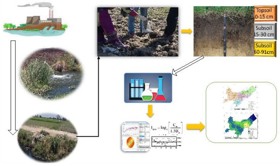
:In third world countries, industries mainly cause environmental contamination due to lack of environmental policies or oversight during their implementation. The Sheikhupura industrial zone, which includes industries such as tanneries, leather, chemical, textiles, and colour and dyes, contributes massive amounts of untreated effluents that are released directly into drains and used for the irrigation of crops and vegetables. This practice causes not only soil contamination with an excessive amount of heavy metals, but is also considered a source of toxicity in the food chain, i.e., bioaccumulation in plants and ultimately in human body organs. The objective of this research study was to assess the spatial distribution of the heavy metals chromium (Cr), cadmium (Cd), and lead (Pb), at three depths of soil using geostatistics and the selection of significant contributing variables to soil contamination using the Random Forest (RF) function of the Boruta Algorithm. A total of 60 sampling locations were selected in the study area to collect soil samples (180 samples) at three depths (0–15 cm, 15–30 cm, and 60–90 cm). The soil samples were analysed for their physico-chemical properties, i.e., soil saturation, electrical conductivity (EC), organic matter (OM), pH, phosphorus (P), potassium (K), and Cr, Cd, and Pb using standard laboratory procedures. The data were analysed with comprehensive statistics and geostatistical techniques. The correlation coefficient matrix between the heavy metals and the physico-chemical properties revealed that electrical conductivity (EC) had a significant (p ≤ 0.05) negative correlation with Cr, Cd, and Pb. The RF function of the Boruta Algorithm employed soil depth as a classifier and ranked the significant soil contamination parameters (Cr, Cd, Pb, EC, and P) in relation to depth. The mobility factor indicated the leachate percentage of heavy metals at different vertical depths of soil. The spatial distribution pattern of Cr, Cd, and Pb revealed spatial variability regarding subsoil horizons. Significant contamination was discovered near the Deg drain and the Bed Nallah irrigated area that indicated a high Cr topsoil contamination, and in a homogenous pattern in Cd and Pb (p < 0.05). Consequently, different soil management strategies can be adopted in an industrial irrigated area to reduce the contamination load of heavy metals in soil.
1. Introduction
Increasing population growth, large-scale industrialization, and exceptional urbanization during the last few decades are responsible for the degradation of the quality of environment and soil [1]. Soil is one of the basic environmental media, it can be contaminated through the accumulation of heavy metals through the discharge of effluents from mine tailings, coal combustion, sewage sludge, disposal of high metal wastes, paints and leaded gasoline, land application of fertilizers, and animal manures [2]. The ill-defined group of inorganic compounds and hazardous chemicals that industries may release and discharge in drains as industrial effluents constitute contamination with different heavy metals, such as arsenic (As), chromium (Cr), lead (Pb), cadmium (Cd), zinc (Zn), mercury (Hg), nickel (Ni), and copper (Cu). Industrial effluents may also lead to the release of heavy metals into the soil that is considered a significant sink media [3]. The availability of heavy metals in soil solution and its downward movement in the profile is highly dependent on the concentration of the particular heavy metal, type of soil, and their physicochemical properties. Metals may be adsorbed on the surfaces of soil particles, precipitate as sulphides, carbonates, oxides or hydro-oxides [4]. Because of the scarcity of fresh water in the arid region, many farmers use industrial wastewater or a mixture of both. This practice has led to a high concentration of heavy metals in soil & soil solution due to the repeated application of wastewater. Soil cannot adsorb such a high concentration of metal when it is released into the soil solution for crop uptake or downward movement in the soil profile and ultimately into the groundwater. The effect of long-term irrigation using wastewater on the heavy metal contents of soil under vegetables in Harare, Zimbabwe was estimated by Manapanda [5].
Soil pollution due to heavy metals is a serious concern because of their toxicological effects on the environment. Heavy metals induced into the soil pose a serious threat to the cultivated soil, vegetables, and food chain, causing human health-related hazards [6]. Heavy metals in soil can cause bioaccumulation in plants and in different organs of the human body through the intake of toxic food [7]. For example, long-term continuous exposure to Cd can cause health issues [8], such as prostatic proliferative lesions, lung cancer, hypertension, kidney dysfunction, and bone fractures. Chronic exposure to an environment that contains Pb may cause symptoms of nephropathy, plumbism, anaemia, central nervous system, and gastrointestinal colic. Different forms of Cr may cause toxicity in the human body. The Cr may exist in many oxidation states, Cr(0), Cr(III), and (VI) valences, which are considered as stable states, while trivalent chromium Cr(III) is naturally occurring in the environment. The Cr(VI) is considered highly mobile and a cause of toxicity [9]. Many industrial processes also cause oxidation and produce Cr(VI) in effluent and industrial wastes. Cr(VI) (hexavalent chromium) is a significant carcinogenic metal for humans, accepted by both the United States Environmental Protection Agency (US-EPA) and International Agency for Research on Cancer (IARC) [10]. Several health risks are associated to Cr(VI), moreover, Cr(III) cannot enter the body’s cells directly: the Hexavalent chromium (Cr VI) may cross the cell membrane and, after entering the cell, it may diminish to Chromium (III), which creates ducts with the DNA and is considered very carcinogenic for health [11]. In agricultural irrigated areas, the spatial dispersal of heavy metals is associated with wastewater, industrial effluents, pesticides, and natural sources.
Heavy metals’ spatial extent and mobility is a critical component to be considered in studies of soil contamination. It is essential to provide detailed information regarding the mobilization, origin, extent, association, and biological availability of toxic metals at different soil depths [12]. The distribution and mobility of heavy metals with regard to soil profile and their bioavailability at different depths of soil for plant growth [13] have been a great concern.
Geospatial analysis techniques are essential tools for the characterization of soil parameters [14]. The implementation of geographic information systems (GIS) using geostatistical and multivariate analysis is an essential method for the evaluation of the spatial structure of heavy metals and the physiochemical properties of soil [15]. Several studies investigated the spatial distribution of heavy metal contamination in the surface soil of industrial areas around the world. For example, Wang et al. reported the spatial disctribution of Cu, Zn, Cr, Cd, As, and Hg concentration in the industrial area in Sichuan, China, were less than the national standards but slightly higher than the naturally occurring baseline values [16]. Ravankhah, et al. conducted an ecological risk assessment of heavy metals in surface soil in the industrial city of Aran-o-Bidgol, Iran [17]. They reported that the concentration of Cd, Pb, Ni, and Cu were higher than the background values. Hossain, et al. compared the spatial distribution of heavey metals in the industrial area with the residental area and reported a higher concentration in the indstrial area [18]. Similarly Agca reported a higher concentration of heavey metals’ (Cd, Cu, Pb, and Zn) spatial distribution around the indutrial area of southern Turkey [19].
Some analyses performed methodical investigations to determine the presence of heavy metals and other elements in soil sediments. They employed conventional statistical techniques to classify soil properties and other factors using a cluster analysis (CA) and a principal component analysis (PCA) [20]. CA and PCA are multivariate analysis techniques and are commonly employed to extract hidden patterns and structures from multi-dimensional data from different fields of the social sciences, natural sciences, and soil sciences [21]. The combinations of these methods are applied for the evaluation and classification of the elements and heavy metals present in soil [22]. However, these methods entail some complexities regarding data analysis from different dimensions with multiple soil depths. Moreover, they require the normalization of skewed results and spatial data distribution patterns that are influenced by many principal components [23]. Therefore, a comprehensive method is required to replace the conventional multivariate statistical methods for the selection of soil parameters with spatial heterogeneity in soil depths. The Random Forest (RF) classifier can accomplish reliable and robust estimations [24] of essential soil parameters at different soil depths. No studies reported a reliable method of assessment for the technique of soil and the ranking of significant soil pollution variables at different depths using the RF classifier of the Boruta Machine Learning Algorithm. In this regard, this article introduces a new assessment of soil parameters at multiple lithological classes of soil depths.
Furthermore, exponential and spherical variogram models have been employed by many experts for the analysis of the spatial variability of heavy metals in soil [25]. For this purpose, apart from the spatial variability of heavy metals at large distances described by the lag distance, the practical interest of variability at short distances is also required for improved characterisation. The Matern constitutes a flexible variogram model with a behaviour of the smoothness and fits the semivariogram close to the origin, supporting the differentiability and continuity of the random variables and covering the local smoothness [26] to plot the sample concentration of soil parameters.
Traditional interpolation methods, such as the Generalized Kriging Method, Polynomial Method, and the Inverse Distance Weighting Method (IDW) have been extensively employed to transform the experimental point data of sample locations into thematic maps that show the spatial distribution [27]. The polynomial method and IDW method are comparatively easy and quick to evaluate, but the spatial variability and relations between the nodes cannot be estimated with them, moreover, these methods allow a partial accuracy of estimation. In comparison, the Kriging Interpolation Method employs the variogram model to analyse the structure of the spatial variation of estimated values and considers the spatial autocorrelation in modelling the surface [16]. The kriging technique comprises a collection of interpolation methods based on stochastic approaches, including ordinary kriging (OK), cokriging, universal kriging, simple kriging, residual, and regression methods [28].
This study applied traditional statistical and geospatial methods, and in addition a novel machine learning approach, i.e., the RF Wrapper function of the Boruta Algorithm, which had not been previously employed in soil contamination studies in the literature. These techniques of analysis were employed to explore the spatial variability of heavy metals not only at the surface soil, but also at the subsurface and deep-soil, and to further assess the mobility factor due to the leaching of heavy metals in the lower horizons of the soil profile.
2. Materials and Methods
2.1. Study Area
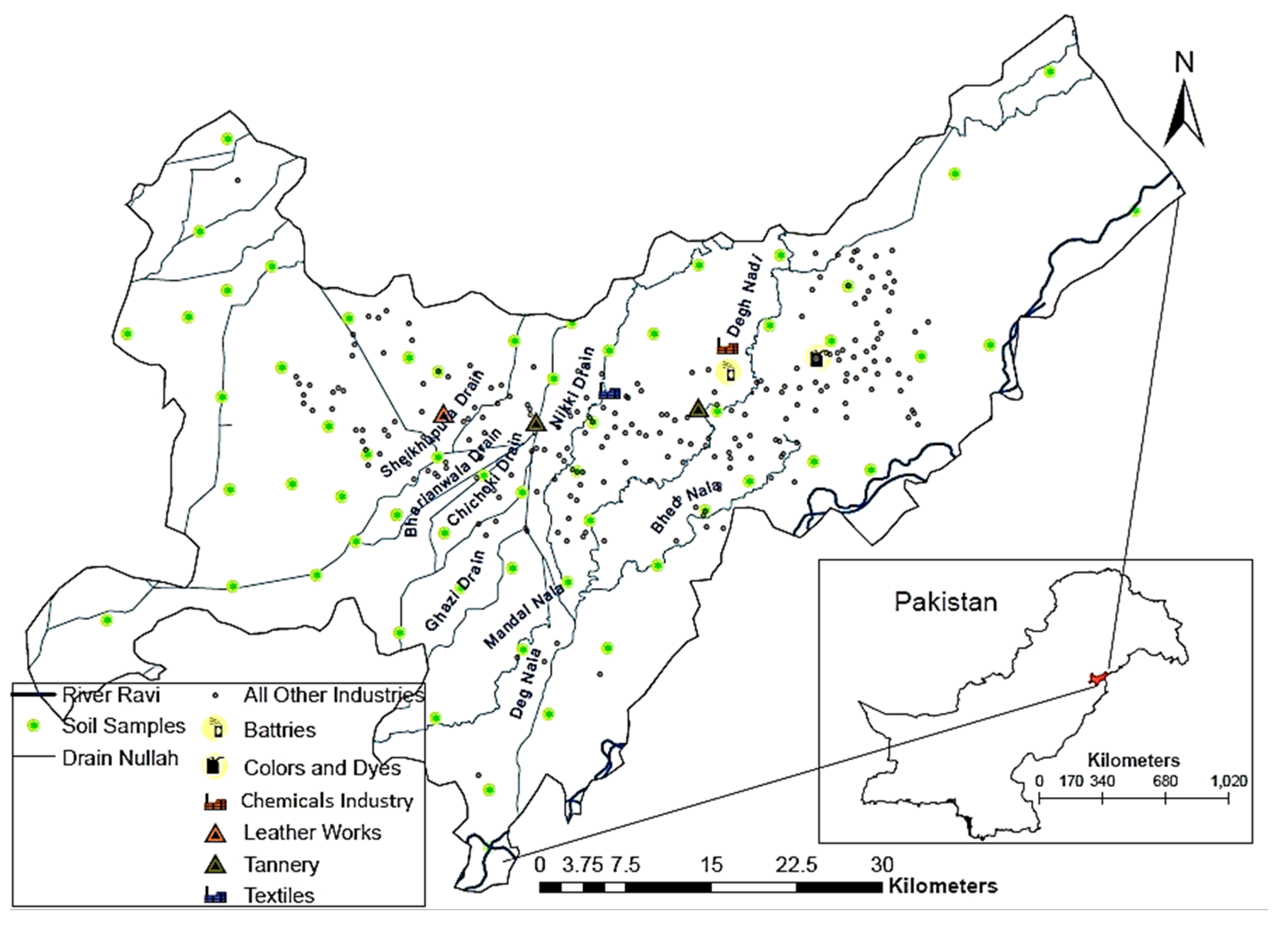
The study area was located in the industrial zone of Sheikhupora (31°20′ N to 33°05′ N and 73°37′ E to 74°41′ E) (Figure 1). A total of 220 major industries are located in this area, which includes tannery and leather, shoes, textile, chemical industries, batteries and tires, rubber, pipe, food, glass, oil and polyester, flour mills, steel mills, rice mils, and fertilizer industries. These industries generate about 395 cusecs of effluent sewage that is released directly into municipal sewers and open surface drains, and ultimately end up in the river Ravi [29]. The discharged effluent contains carcinogenic and hazardous substances and a high level of heavy metals, aromatic dyes, inorganic salts, and organic material [30].
2.2. Soil Sampling and Lab Analysis
A random soil sampling technique was employed for the collection of soil samples to make sure that all sites in the study area were represented in the soil sampling [31]. A total of 60 sites were sampled at three depths (0–15 cm, 15–30 cm, and 60–90 cm) and a total of 180 (60 × 3) soil samples were collected with a tube auger (Figure 1). Each soil sample was represented by three replicates that were composited as a single sample. The spatial coordinates of the sampling locations were recorded using a handheld Garmin Global Positioning System (GPS).
The collected soil samples were placed in labelled paper bags and transported to the lab for further analysis. The soil samples were dried, and subsequently, crushed and passed through a fine sieve of 2 mm [32]. Soil chemical properties including EC, pH, P, K+, and saturation were determined in soil samples using the standard procedures [33,34]. Soil organic matter (OM) was determined through Tyurin’s method [35,36]. The acid digestion method followed by USEPA standards 3051A and 3050B was employed to evaluate the total concentrations of selected heavy metals in the soil samples [37,38]. Further, the digested soil samples were analysed for the selected heavy metals (Cr, Pb, and Cd) using the Graphite Furnace Atomic Absorption Spectrometer (GFAAS) by means of their respective wavelengths [39,40]. The metal concentrations were expressed in units of mg kg−1 of the dry soil. The concentrations of all examined physiochemical properties and selected heavy metals for the three depths of soil were arranged along with their spatial coordinates in ArcGIS Geodatabases. The soil data was further explored using exploratory data analysis techniques.
2.3. Descriptive Statistics and the Correlation Matrix of Soil Parameters
The heavy metals present in the soil and other chemical properties were statistically analysed using the SPSS software (IBM Corp., Armonk, NY, USA) [41] to determine the descriptive statistics (max. min., standard deviation, kurtosis and skewness) and coefficient of correlation. The distribution pattern of all parameters for the three depths of soil was estimated based upon the SD and skewness values. Datasets of a variable with skewness in the range −1 and 1 were considered to be normally distributed [42].
2.4. Selection of Soil Parameters Using the Random Forest Classifier
In order to classify the soil parameters according to their variability or consistent distribution patterns at different soil depths, a feature selection of algorithm Boruta [43] was applied with the Classifier (RF) function. The RF classifier is a machine learning function of the wrapper method through the Boruta algorithm [44]. The wrapper function of RF identifies relevant parameters by performing multiple runs of the provided classification factors that test the performance of different subsets of the input parameters [45]. The RF function is a suitable alternative for the analysis of soil parameters at different depths, as it can be employed without extensive parameter tuning and returns an estimate of the feature’s importance (Z-score) [46]. This parameter selection method is different from other dimensionality reduction techniques, such as PCA or other methods. The purpose was to identify the compound linkages of the concentration of heavy metals in the geographical context of the soil profiles. Unlike the PCA, this method attempts to reduce the number of attributes in the dataset, without reducing the dimensionality [47].
In the present scenario, the soil’s physio-chemical parameter (soil saturation, EC, OM, pH, P & K) and heavy metals (Cr, Cd, and Pb) were evaluated using the RF, while soil depths were assigned as the classification factor. Therefore, it was likely to identify the effective random soil parameters that may explain some of the variability in the targeted classes of soil profile by obtaining the positive Z-score by a single run of the RF classifier (Equation (1)).
where PPV∗ represents the approximate positive predicted values, Nrelevant (Xcontrast), and Nrelevant (Xoriginal) constitute a number of contrast and original variables respectively, which the algorithm considered significant. The importance scores of the original features were tested against these random variables and only parameters with a positive higher Z-score were retained as significant soil variability factors. The analysis was repeated for each depth of soil (0–15 cm, 15–30 cm, and 30–90 cm) to check the robustness of the parameters for the contamination risk at the subsoil level. This may examine the possibility of selected soil heavy metals for quantification according to their mobility at different depths.
2.5. Metal Mobility Ratio in Subsoil Profiles
A metal mobility factor (Equation (2)) was utilised to differentiate the natural concentration of heavy metals at different soil depths [48] from the anthropogenic contamination. The metal mobility factor describes the possible movement of the selected heavy metals out of the soil profiles [49].
where MMR denotes the metal mobility ratio, and M represents a concentration of metals (Mt1, Mt2, and Mt3 indicate total heavy metal concentration in the soil, Ma4, Ma5, Ma6 indicate available heavy metal enrichment for plants) at the three different fractions of soil depths. The mobility ratio of selected heavy metals (Cr, Cd, and Pb) denotes the vertical distribution of soil contamination parameters at different depths; however, to assess the variability and spatial distribution of heavy metals in the soil, the geostatistical approach was further employed to map the geographical extent of heavy metals.
2.6. Geostatistical Analysis and Variogram Modelling for Soil Heavy Metals
The spatial distribution of selected soil heavy metals (Cr, Cd, Pb) at different depths was assumed as a normal random distribution and was assessed using variogram modelling. Spatial distribution maps were generated to depict the spatial variability of heavy metals. Four variogram models (Matern, Spherical, Exponential, and Gaussian) were tested. The Matern (Ste) variogram, which had the smallest root mean square error (RMSE), was optimally suited and selected. Experimental variograms were estimated and fitted with the theoretical models. If a variogram reaches a certain limit that results in a certain effective range, the spatial structure and conditions for inherent spatial assumption can be achieved. The Matern variogram models were calculated [25] using the given Equation (3).
where > 0 represents the variance, > 0 is the shape parameter, > 0 represents the scale (or range) of parameter, (.) forms the modified Bessel function of the second kind order, (.) represents the gamma function, while and constitute the norm of vector h, v = 0.5. Further, the Matern model is the exponential model, while the Gaussian model represents a limiting case of the Matern model when n tends to infinity [50]. The variograms were calculated for the nine different parameters of soil at the three soil depths. The maximum sample variogram distance, taken from 1/3 of the range parameter, sill displayed the spatial autocorrelation component. The nugget parameter was assumed as the mean of the first three sample variogram values. The partial sill was assumed to be the mean of the last five sample values of the variogram and scaled through variance values. Furthermore, based on estimation and the smallest RMSE, the Matern variogram was considered as a suitable model to predict the spatial surfaces of heavy metals’ concentration, except for Cr (15–30 cm), for which the spherical variogram was selected as the suitable model.
Kriging Interpolation
Spatial prediction to assess the variability of parameters implies the process of estimation of a target quantity’s values at un-sampled locations. Ordinary kriging (OK) interpolation is the geostatistical method employed for the spatial distribution of heavy metals’ concentration (Cr, Cd, and Pb) in soil at three depths. It entails the superior method for the estimation of interpolation weights and can provide error information for the creation of the thematic maps. The following formula was used to estimate the OK:
where . represents the interpolated or predicted value for S0 point, and . is the value for the equivalent weight of the values, while indicates the known value to satisfy the condition and = 1.
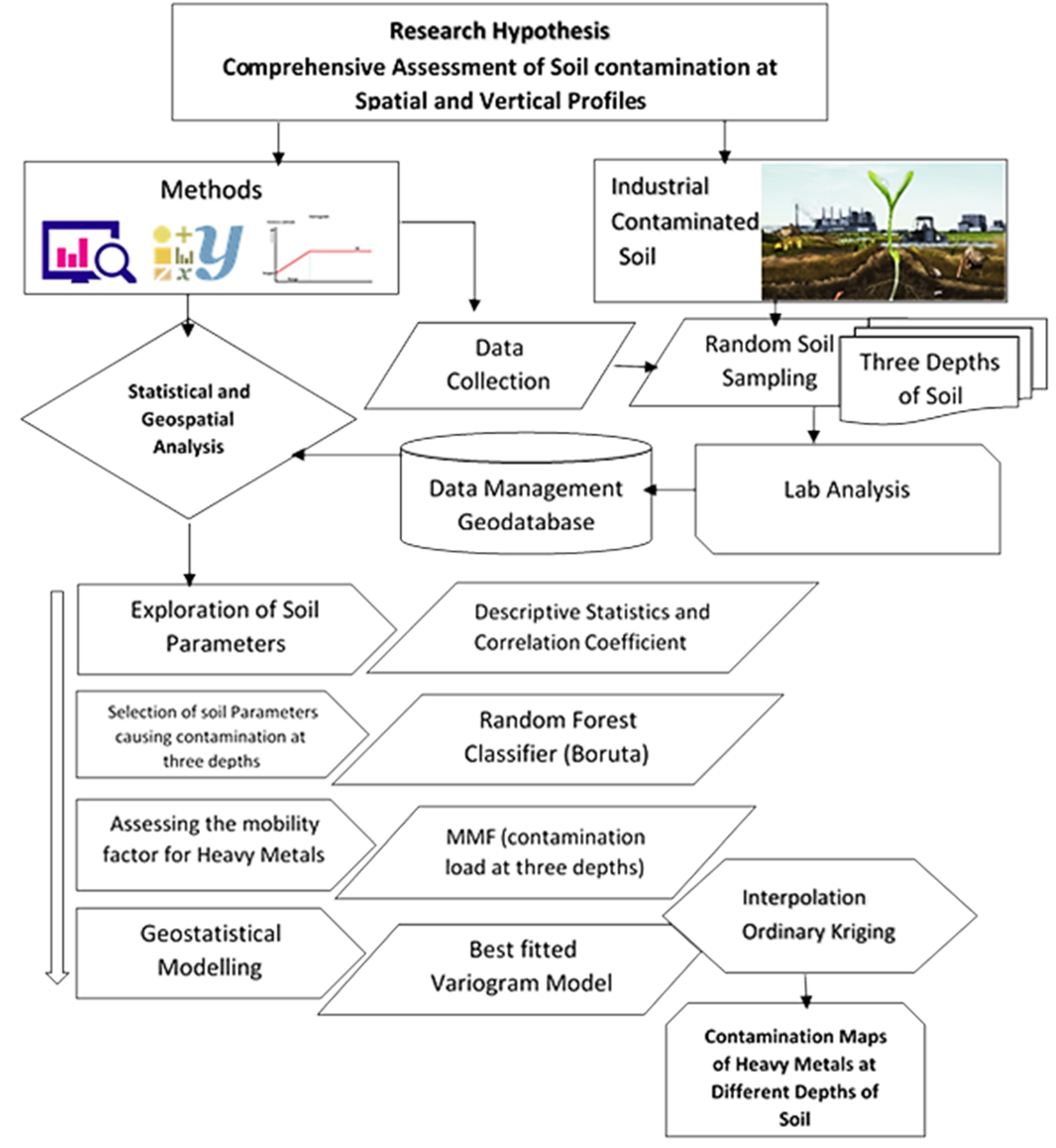
The SPSS software was utilised for the statistical analysis, GeoR (version 3.3.3) [51] the gstat package was used for the geostatistical analysis, and ArcGIS (ESRI, Redlands, CA, USA) [52] was applied for the interpolation of the distribution maps for heavy metals in soil [53,54]. Figure 2 presents the complete methodology flowchart.
3. Results and Discussion
3.1. The Exploratory Analysis of Soil Variables
Table 1 presents the descriptive statistics of all the soil variables. All the variables display a normal distribution, except potassium (K) (skewness value > 2) and EC (skewness = 1 in topsoil and subsoil; < 1 in deep-soil). The mean concentration of EC for the topsoil was significantly (p < 0.05) higher than that for the subsoil and deep-soil horizon. The mean pH (8.2–7.8) and EC values (4.9–4 µS cm–1) exhibit a decreasing trend from the topsoil to the subsurface soil. The order of heavy metal concentration in the soil was Cr > Pb > Cd, with a decreasing trend from the surface to the subsurface soil (Table 1). The heavy metals’ assimilation can be greatly influenced by the physiochemical properties of soil that, ultimately, also affect the root growth and mobility of the contaminants at different soil horizons [55].
The P concentration significantly increased from the topsoil to the subsoil (range 17.3–20.3 mg kg–1). Andersson found high P concentrations at the subsoil, as compared to the topsoil, that indicated that the subsoil acted as a sink or source for P leaching. Therefore, depending on the P concentration and the soil saturation level, the subsoil properties could be considered for the adoption of mitigation measures to reduce the P leaching in soil horizons [56].
Table 2 presents the results of the correlation coefficient for various soil properties. A positive significant (p ≤ 0.01) correlation coefficient (r = 0.55) was found between pH and EC. However, a non-significant (p ≥ 0.05) relationship (r = 0.12) was found between OM and pH, and a negative correlation was found between all heavy metals and pH. Many laboratory experiments and studies demonstrated the existence of a negative correlation coefficient between the mobility of heavy metals and pH [57]. A significant correlation was assessed between all three heavy metals and P, while OM indicated a positive relationship with Cr and Pb, but a negative non-significant (p ≥ 0.05) correlation with Cd. A negative correlation between Cd and Pb was discovered with soil saturation, while a positive correlation was found with Cr. The Cr with its oxidation states may affect greater downward mobility in the presence of high soil saturation [58]. Generally Cr is highly mobile in soil, however, Cr(VI), due to its anionic nature, can be adsorbed by clays, iron and manganese oxides and hydroxides in acidic soil because of an increase in positively charged sites at mineral surfaces [59]. The retention of Cr(VI) decreases with increasing pH, resulting in higher mobility in the subsurface soil due to weak adsorption in the alkaline to neutral conditions [60]. Similarly, Pb and Cd solubility and movement is highly dependent on soil pH and the type of soil separates. Both metals are highly available naturally at low pH, but since the study site is repeatedly irrigated with the wastewater enriched with the heavy metals, the concentration will govern its bioavailability and movement in the soil [61]. The metal to metal correlation indicated the mutual variability in metal accumulation and their bioavailability in soil [62]. The random pattern of correlation among each soil parameter is observed from each layer of soil. Therefore, to check the relevance and importance of each soil parameter with regard to soil depth, a wrapper algorithm with the RF classifier [63] was employed using the R package Boruta [46].
3.2. Assessment of Soil Contaminant Parameters
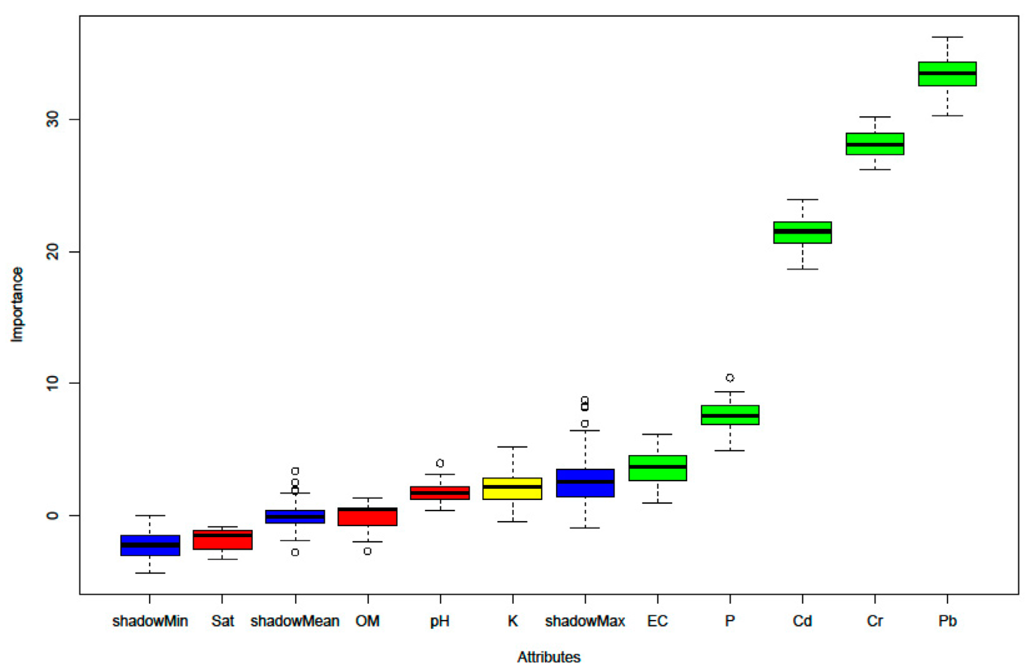
Further investigation of the soil parameters was required to sort and denote the soil contamination factors with regard to the downward soil profile at the random spatial scale. Therefore, a combination of multiple parameters (parameters = 9 and depths = 3) were tested and assessed with the wrapper RF Boruta algorithm that performed three iterations based on different classes of soil depths to attain reliable soil contamination plots for the study area. The outcomes associated with this method confirmed the relative significance values of all soil parameters (soil saturation, EC, OM, pH, P & K, and Cr, Cd, and Pb) in this study. In Figure 3, the Y-axis represents the Z-score values to discriminate the importance of each soil property (X-axis) for the given random samples. The significance of the soil parameters was evaluated with regard to spatial distribution and downward availability from the topsoil to subsoil profiles, and the relative importance factor was assessed as Z-scores ≥ 1. The blue boxes represent the shadow variables. In RF, randomness is assigned to the data, and the shuffle copies of all parameters are created as shadow features. At every iteration of soil depth, whether a real soil parameter had a higher critical score than its shadow feature was determined.
Large Z-scores of a parameter indicated significant (p ≤ 0.05) importance. The distribution of Pb was found to be random with substantial importance (Z ≥ 30) which showed significant permutations in comparison to other heavy metals (Cr ≤ 30 and Cd ≥ 20). This indicates that the concentration of heavy metals has higher Z-scores based on permutations of spatial variability and the heterogeneity of metals at different soil depths [64]. The importance of P was also found to be significant (p ≤ 0.05, Z-score ≤ 10) in the consideration of the soil analysis with RF, it is the critical nutrient in soil and vastly used in agricultural soil as a fertilizer [65] and showed significant leaching from topsoil to subsoil (p ≤ 0.05). The RF importance score for EC with Z-score ≥ 1.0 implies the least significance (10%) as compared to other significant soil parameters. The importance of score K is estimated as a tentative parameter by a simple comparison of the median attribute, which was not confirmed as significant. The saturation (Sat), OM, and pH were indicated as not confirmed by the RF (p ≥ 0.05), which may indicate some assortment of soil horizons with the least important Z-score (≤1.0). Furthermore, it is evident that the soil parameters that invariably yielded the high importance Z-scores in each class of soil depth during the individual RF runs were selected as important. The classification performance and assortment of soil parameters was directly affected by the permutation process of the RF. The relatively high importance factor revealed its permutations by using the RF algorithm. Since the whole process is dependent on permutation without reducing the dimension, dimensionality reduction techniques such as PCA [66] were replaced by RF to explore the distribution of soil parameters at depth. Additionally, the mobility assessment of important soil heavy metals at the individual level is necessary for further investigations at subsoil horizons.
3.3. Estimation of Metal Mobility and Variability at Vertical Soil Profile
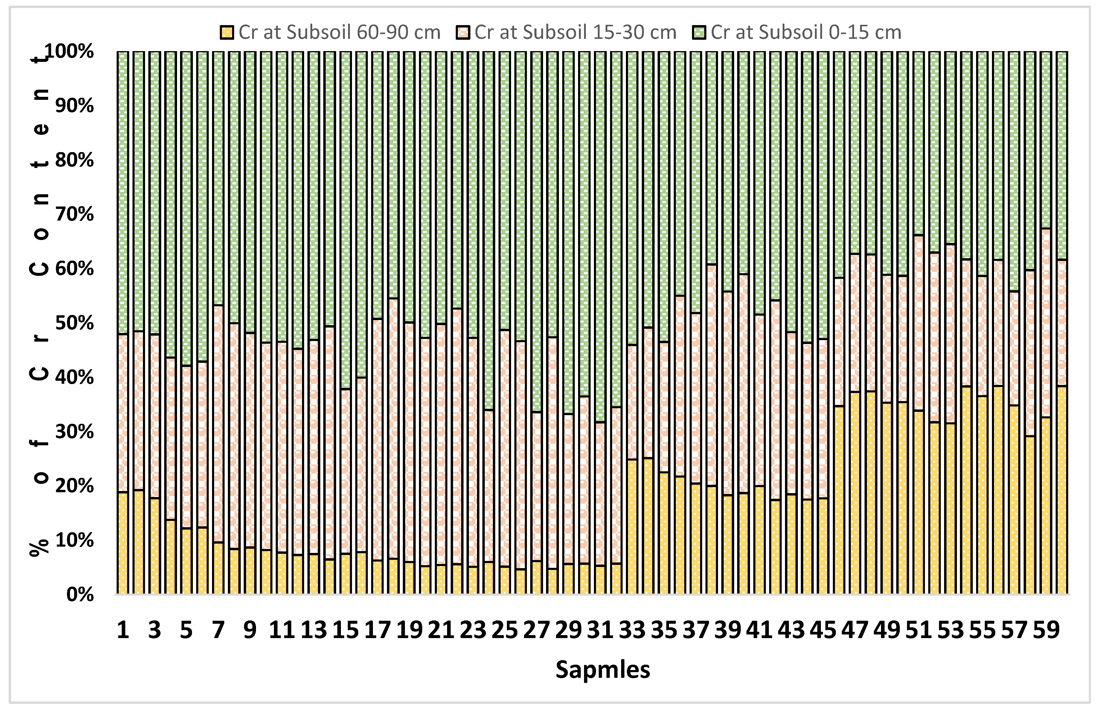
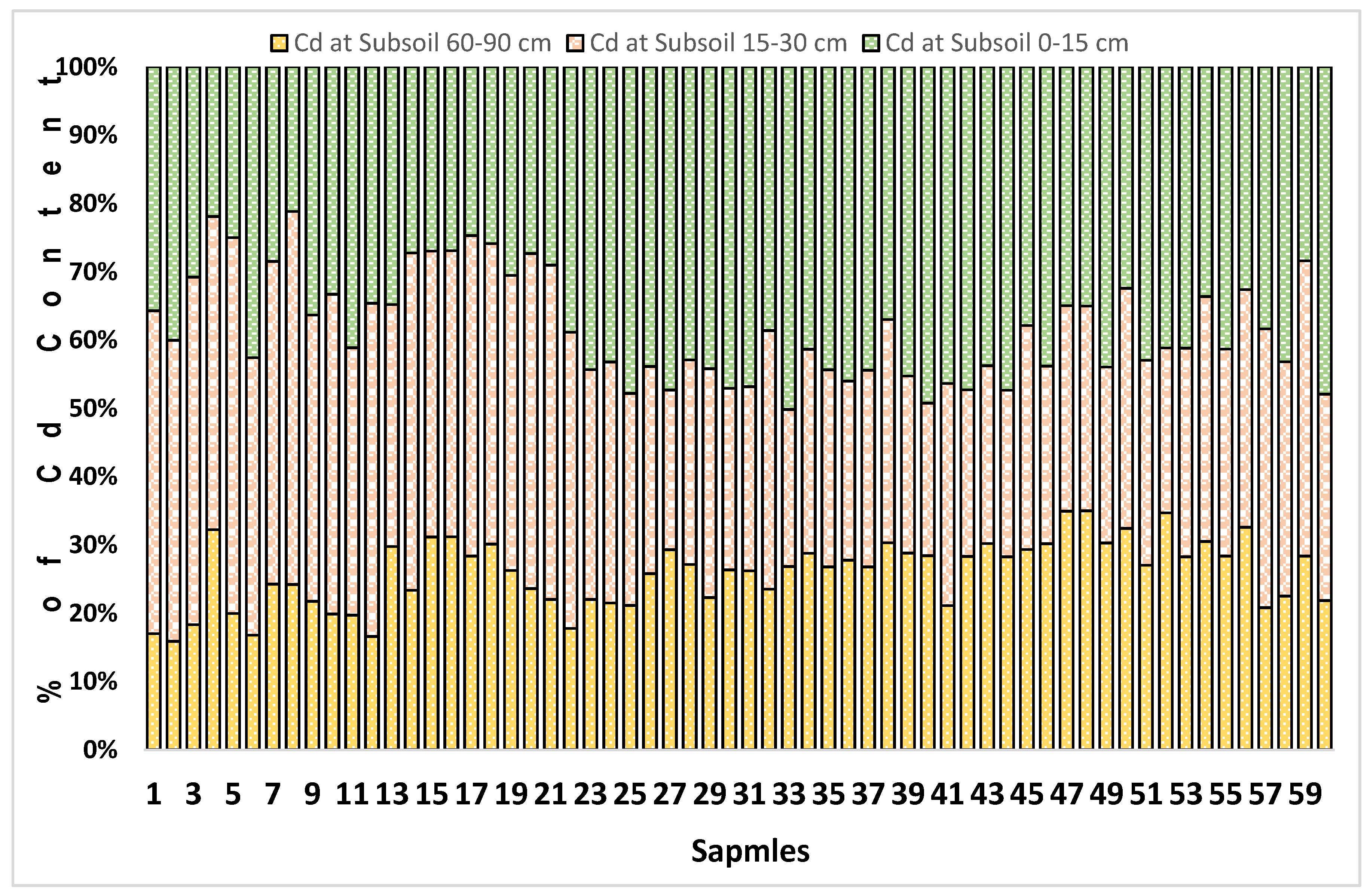
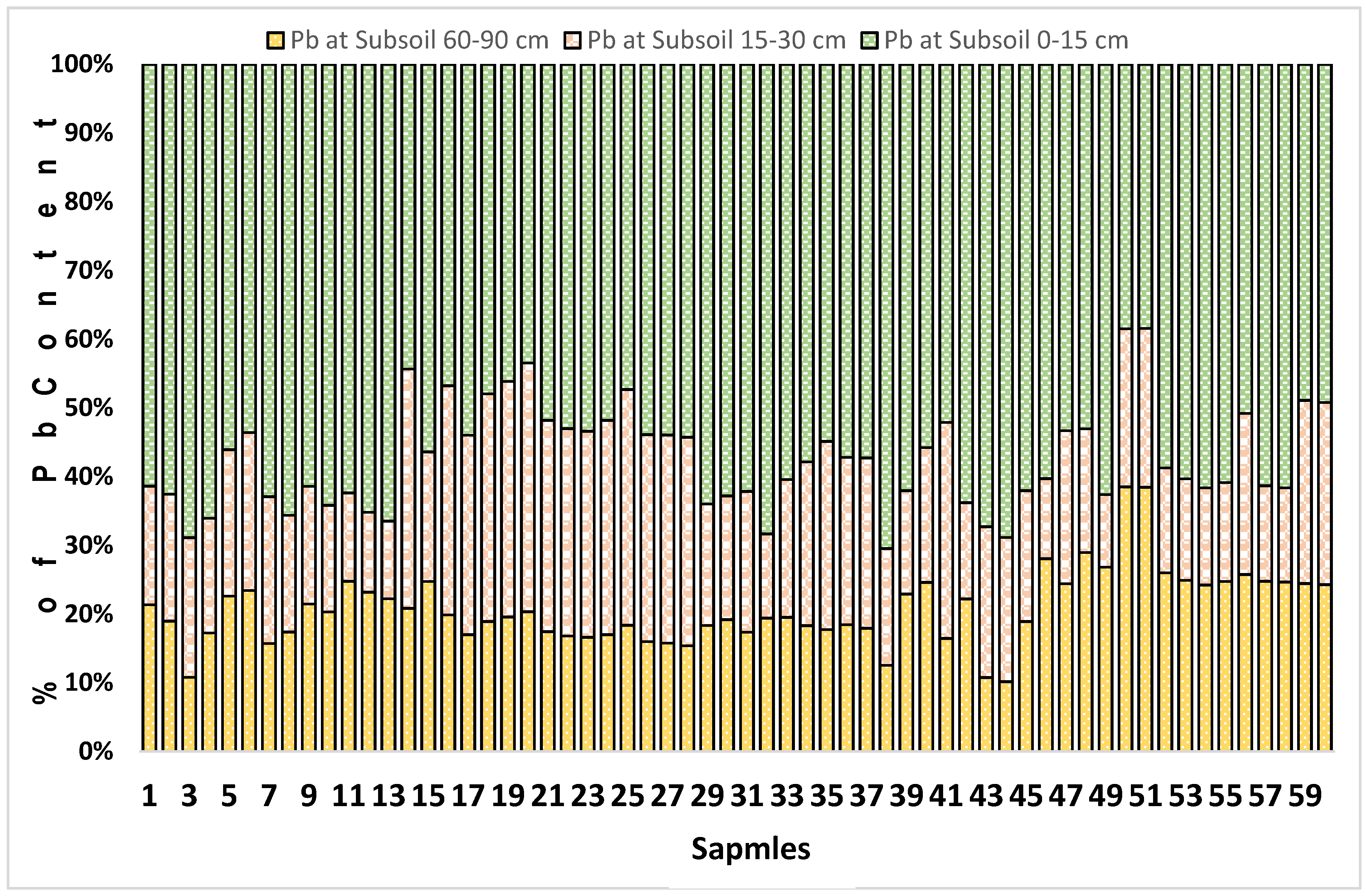
For the RF classifier, the heavy metals were selected as essential contamination factors with significant speciation at different soil depths. The degree of contamination and downward percolation of heavy metals in soil was assessed using the metal mobility ratio. The mobility ratio of the total heavy metals’ concentrations and environmentally available metals’ concentrations at different depths were assessed. The metal mobility ratio was calculated for the leachate of Cr, Cd, and Pb at three different depths of soil. Figure 4 revealed that the topsoil contained >50% mobility for Cr, while for the middle soil, the value of metal mobility ratio (MMR) was 30%, and 0–20% MMR for subsoil. The mobility of Cd was 40% at the topsoil profile, while there was >45% mobility in the middle soil depth and >20% mobility at subsoil (Figure 5): this indicates the highest speciation of Cd below the surface soil. Pb displayed the highest mobility at the topsoil horizon, with >60% MMR, while it was 20% in the middle and subsoil MMR. This demonstrates a low leachate of Pb in the deep-soil (Figure 6). The concentration of heavy metals that can pose a danger to the ecosystem and plants was represented as the environmentally available level. The comparison of the available and total concentrations of heavy metals in the three soil depths indicated that the mobility ratio of Pb is higher than that of Cr and Cd. Furthermore, the percentage of water-soluble Cd concentration in the subsoil was higher than that obtained for the effluent irrigated topsoil. The concentration of Cr indicated more water-soluble, exchangeable, and carbonated bound forms in the topsoil profile [67]. The heavy metals’ speciation and their mobility associated with toxicity at soil depths were critical to understand and evaluate the bioavailability of environmental risks. However, various variogram models for each heavy metal were evaluated for all three depths before generating their respective spatial interpolation maps.
3.4. Assessment of Appropriate Variogram Models
The spatial analysis of heavy metals in soil is considered as a prerequisite for designing effective strategies for the improved management of contaminated soil [68]. For that purpose, the selection of the best-fitted variogram model to explore the spatial structure, and ultimately, generate accurate perdition maps at the un-sampled location is required. The variogram models for the soil heavy metals were estimated based on cross-validation. The best-fit parameters of the variogram models are presented in Table 3. The best-fit experimental variogram models were selected based on the lowest RMSE values obtained by the GeoR software.
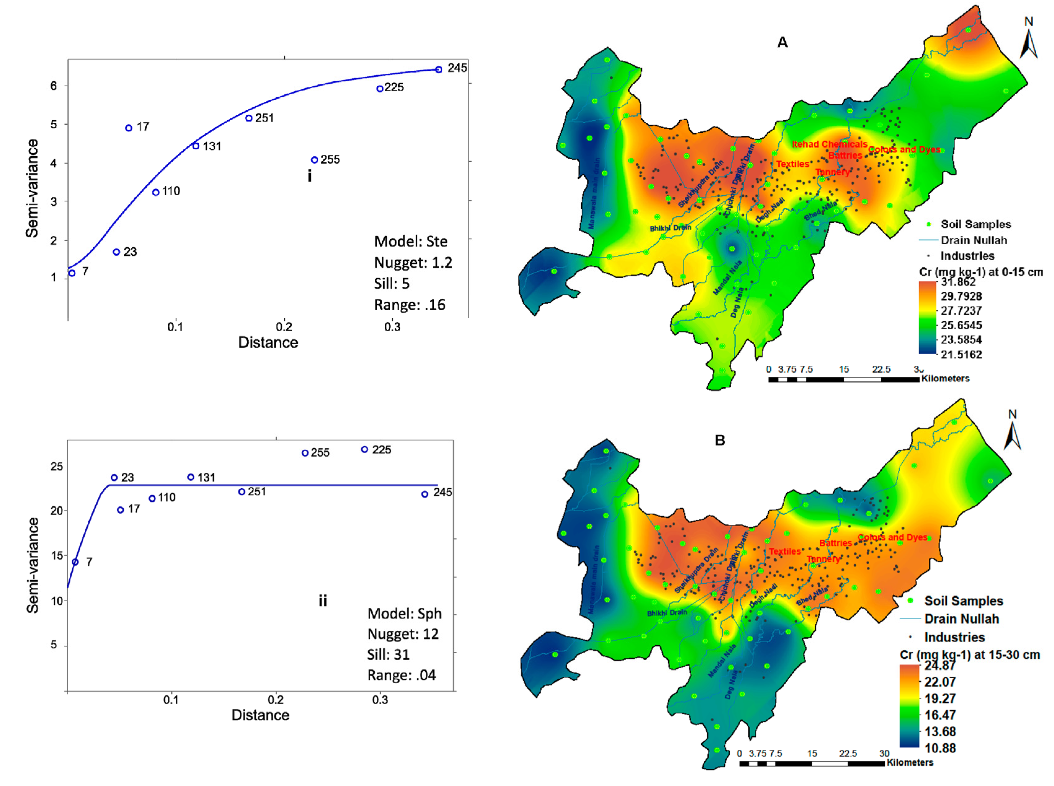
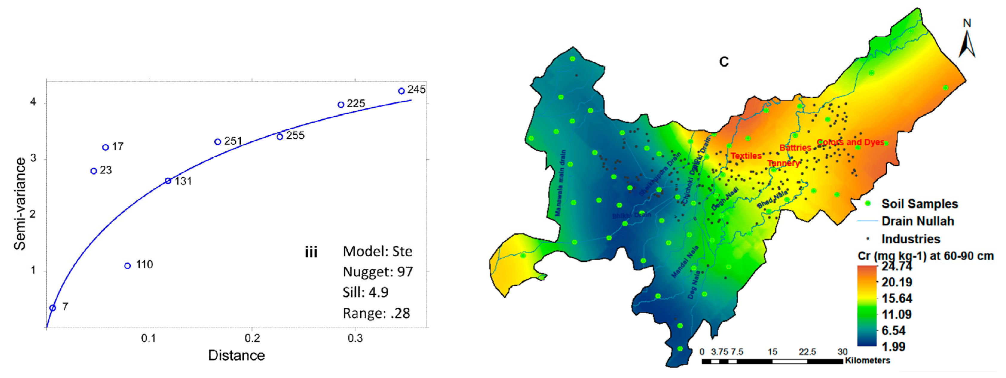
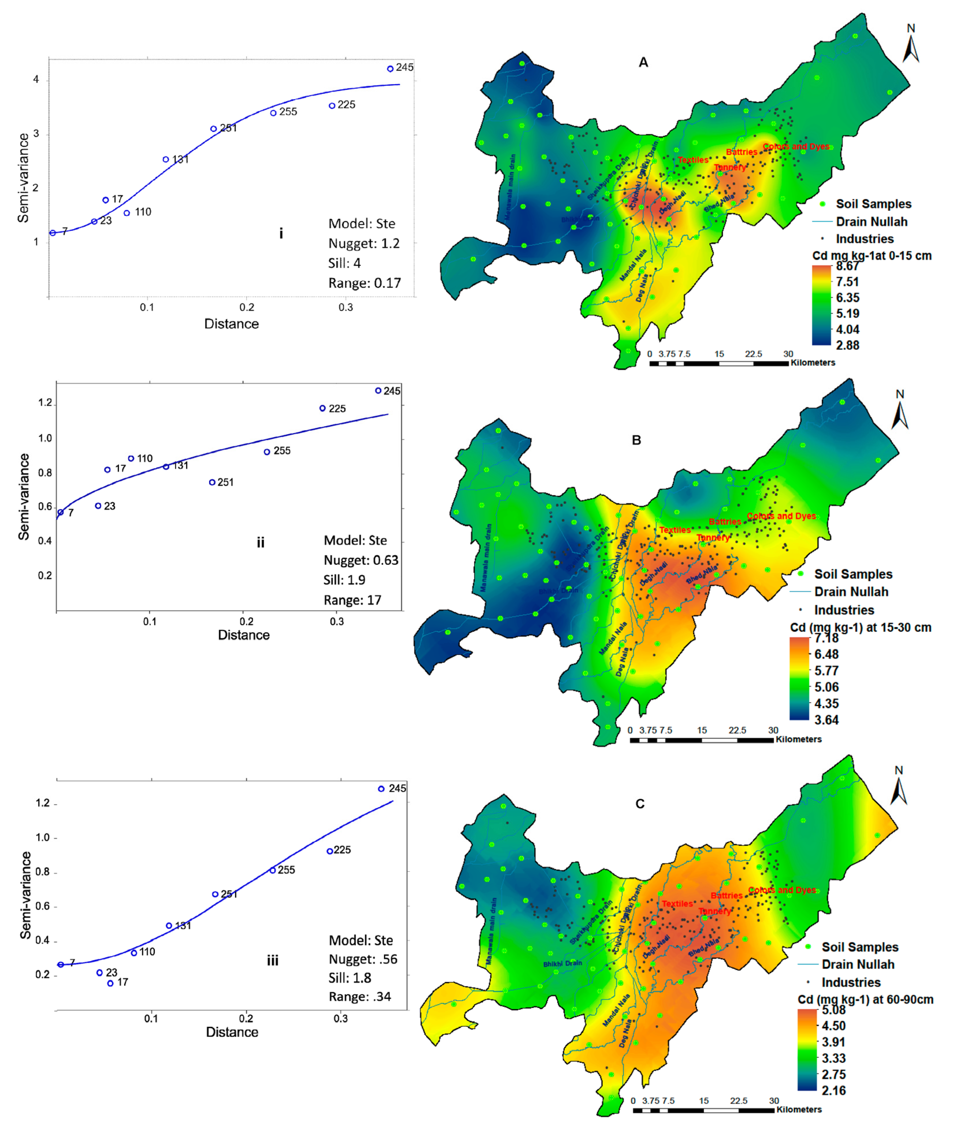
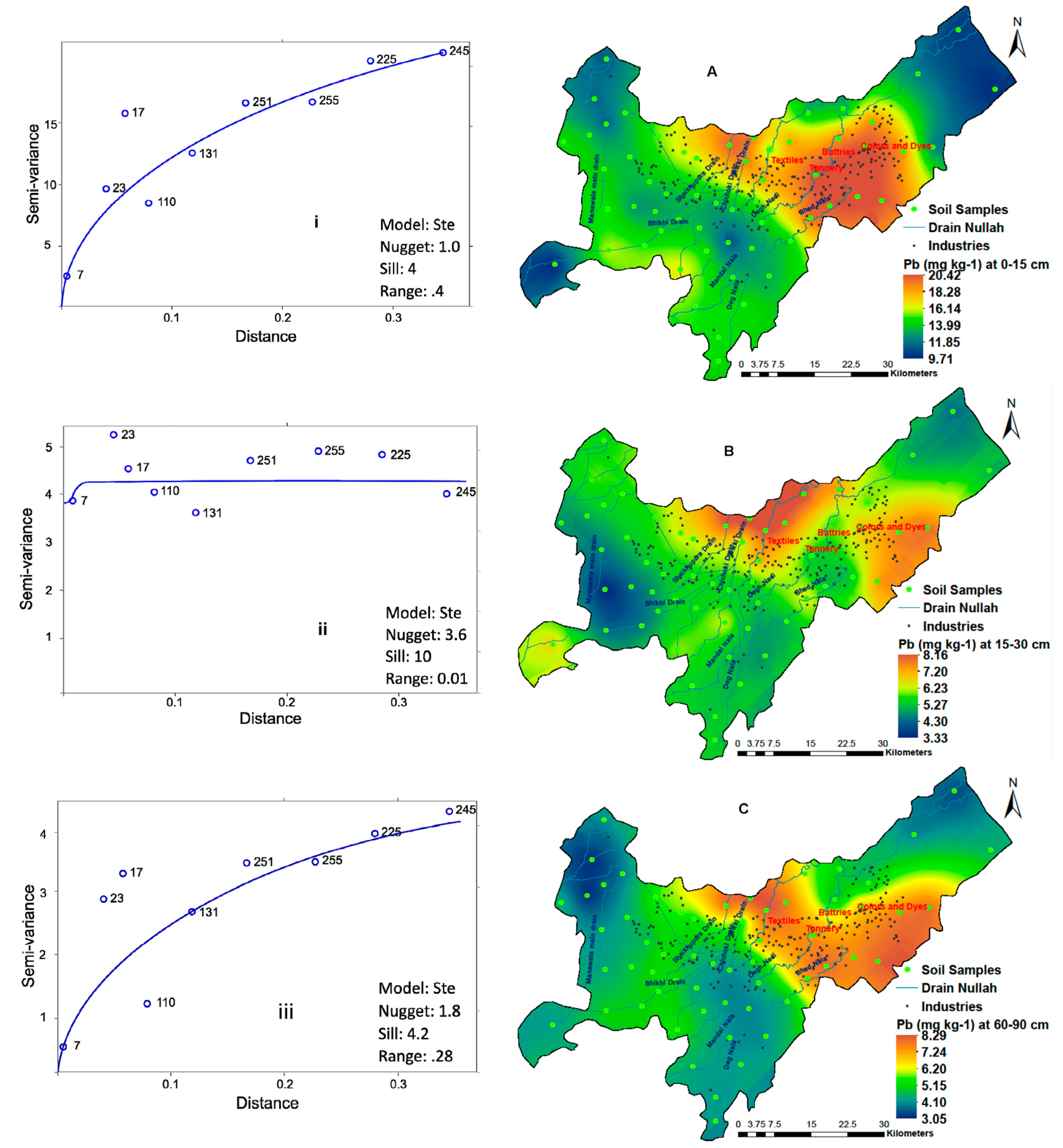
The spatial correlation of the soil heavy metals was assessed through the estimation of the ratio of the nugget effect in relation to the sill. A variable was considered to be strongly spatially dependent if the ratio was ≤ 25%; moderately spatially dependent if the ratio ranged between 25% and 75%; and weakly dependent if the ratio exceeded 75%. The heavy metals’ concentration was indicated to have a moderate to weak dependency for the spatial variability on the topsoil to subsoil profiles. Therefore, it indicated that the concentration of heavy metals at the subsoil profile is affected by the slow leachate process. High soil saturation, with less permeability and a high porosity of soil at the deep-soil level, may also affect the variability [69]. The variogram of Cd (60–90 cm soil depth) (Figure 7ii,iii) showed some fluctuations with a small upward trend with a low sill, suggesting that there is less spatial autocorrelation. This may lead to heterogeneity in the spatial distribution of Cd. The variograms for the concentrations of Pb (Figure 8i–iii) and Cr (Figure 6i–iii) are normally well structured with small nugget effects, demonstrating that the sampling density is acceptable for the spatial structures with moderate spatial dependency. According to the nugget/sill ratios of heavy metals’ (Cr, Cd, Pb) concentration, the selected variograms were found to be suitable for the adoption of interpolation techniques to predict attribute values at un-sampled locations using related information.
3.5. Spatial Distribution of Heavy Metals in Soil
The spatial extent of the Cr concentration reveals a homogenous trend in the topsoil (Figure 7A) and subsoil (Figure 7B) around the tanning industries in the (northern) N and (western) W part of the study area. In the topsoil, high concentrations of Cr in the eastern (E) part of the study area exhibited trans-boundary chromium discharge in drains from the tanning industry in the neighbouring areas [70]. An extensive amount of untreated effluent containing chromium is discharged by the tanning industries and released directly into the drains for irrigation purposes [71]. Figure 7C reveals a different spatial trend for Cr with E to W, with a maximum concentration of 20–24 mg kg–1 in deeper soil profiles that indicate Cr leached into the deep-soil from the anthropogenic source. The Cr percolation may vary with different valent stats of metal through the processes of oxidation and reduction [72]. The spatial extent of Cd displays a higher concentration in the central part of the study area in patches while it covers greater spatial extent of higher values in subsoil and deep-soil (Figure 8A–C). It showed the highest Cd concentrations, ≥8 mg kg–1 in Figure 8A topsoil, ≥7 mg kg–1 in Figure 8B subsoil, and ≥5 mg kg–1 in Figure 8C deep-soil at the central part, with a south (S) and S-E trend of Cd around the industrial zone of the study area. While, a medium concentration (≤5 mg kg–1) was found in the extreme eastern part at all soil depths. Low concentrations (≤4 mg kg−1–≥2 mg kg−1) were found in the W parts for the topsoil and the subsoil. While a ≥2 mg kg–1 Cd concentration was found in the N-W part and ≥3 mg kg−1 in western parts of the deep-soil. There was a narrow outlier of high Cd concentrations in the extreme W portion of the study area that may be associated with the industrial point source pollution, such as the Cd battery production plants indicated in Figure 8C. The Cd concentration decreased spatially from top to deep-soil layer, however, the subsoil formed a transitional layer with similar distribution patterns while the deep-soil demonstrated more stable and consistent deposition of Cd, and the same was reported by Onweremadu [73]. The Pb in all three depths of soil revealed higher concentration in the N-E quadrant (Figure 9A) of the study area, while a small-scale discontinuity pattern of Pb was found with a concentration level of 6 mg kg−1 (Figure 9B) in the subsoil. The patterns of medium and low concentrations in Figure 9C were observed under the lead emission drain that form slow sinks of Pb in the deep-soil profiles [74].
The overall heavy metals’ concentration maps revealed that high amounts of Cr, Cd, and Pb were found in soil profiles in the north direction and the central part of the study area. This area is subject to the discharge of different drains that carry industrial effluents that are used to irrigate the agricultural fields. This causes heavy metal emission in the soil, with a continuous uptake of contamination [75]. Clusters of many industries were discovered in the study area based on our survey that constitutes the source of untreated wastewater. The industries and the discharged effluent waste form the major possible sources of the leading extrinsic factors responsible for a high concentration of heavy metals in soil in this area.
This research would be instrumental in the assessment of heavy metals’ contamination of soils and their remediation strategies. The reclamation of contaminated soil with heavy metals at different depths can be achieved with an appropriate understanding of the trends, availability, and leaching of metals downward. Further, heavy metal contamination can be assessed at subsequent groundwater levels, in cultivated plants, and humans. Scientific information regarding the spatial variance of measured soil properties is essential for the formulation of sustainable soil and environmental management decisions [76].
4. Conclusions
Continuous effluent discharge contaminates the soil in the vicinity of industrial areas. It was discovered in this study that soil is being contaminated with the continuous loading of heavy metals at different levels. The EC values were found to be low from the topsoil to the subsoil and exhibited negative correlations between heavy metals, while they shared a positive correlation with pH. However, pH and EC were found to have a negative correlation with all the heavy metals. The RF function was found to be extremely useful for assortments that possess a significant variability in subsoil horizons without changing or reducing the parameters. In the RF EC, P, Cr, Cd and Pb were found as significant (p ≤ 0.05 and Z score ≥ 2) soil parameters across all soil depths. The soil mobility ratio identified the different percentages of heavy metal leachate with a downward vertical scale. The spatial extent and geographical distribution pattern of the heavy metals were assessed through the geostatistical technique of kriging, based upon the most suitable variogram model. The variogram modelling for the soil contamination sorted at three different depths of soil and the spatial distribution of heavy metals provided a comprehensive depiction of soil pollution in the industrial area. The N-W and central part of the study exhibited maximum contamination at all soil depths. This, therefore, constituted the major effluent irrigated area for raising crops and vegetables. It is recommended that agriculture crops and vegetables are not irrigated with waste water, to eliminate the toxic effects that it may have on humans. Instead, it should be used for non-food crops. Further research is needed to assess the concentration of heavy metals in the groundwater, field crops, and their impact on human health.
Acknowledgments
National University of Sciences and Technology (NUST), Islamabad provided financial support for data collection, laboratory analysis and article processing fee in an open access journal. The authors also acknowledge Ijaz Hussain and Zulfiqar Ali, Department of Statistics, Quaid-e-Azam University, Islamabad, Pakistan for providing guidance in the statistical analysis.
Author Contributions
Asma Shaheen, first author, has done original work based on different modules by data collection, experimental, and other geospatial analysis under the supervisor of Javed Iqbal. He has corrected and evaluated the manuscript and guided in all the phases of research with full supervision.
Conflicts of Interest
The authors declare no conflict of interest.
References
- Saha, N.; Rahman, M.S.; Ahmed, M.B.; Zhou, J.L.; Ngo, H.H.; Guo, W. Industrial metal pollution in water and probabilistic assessment of human health risk. J. Environ. Manag. 2017, 185, 70–78. [Google Scholar] [CrossRef] [PubMed]
- Zhu, Y.; Zhang, Z.; Zhao, X.; Lian, J. Accumulation and potential sources of heavy metals in the soils of the Hetao Irrigation District, Inner Mongolia, China. Pedosphere 2017, in press. [Google Scholar] [CrossRef]
- Cai, L.; Xu, Z.; Ren, M.; Guo, Q.; Hu, X.; Hu, G.; Wan, H.; Peng, P. Source identification of eight hazardous heavy metals in agricultural soils of Huizhou, Guangdong Province, China. Ecotoxicol. Environ. Saf. 2012, 78, 2–8. [Google Scholar] [CrossRef] [PubMed]
- Moral, R.; Gilkes, R.; Jordán, M. Distribution of heavy metals in calcareous and non-calcareous soils in Spain. Water Air Soil Pollut. 2005, 162, 127–142. [Google Scholar] [CrossRef]
- Mapanda, F.; Mangwayana, E.N.; Nyamangara, J.; Giller, K.E. The effect of long-term irrigation using wastewater on heavy metal contents of soils under vegetables in Harare, Zimbabwe. Agric. Ecosyst. Environ. 2005, 107, 151–165. [Google Scholar] [CrossRef]
- Yang, J.; Lv, F.; Zhou, J.; Song, Y.; Li, F. Health risk assessment of vegetables grown on the contaminated soils in daye city of Hubei Province, China. Sustainability 2017, 9, 2141. [Google Scholar] [CrossRef]
- Stankovic, S.; Kalaba, P.; Stankovic, A.R. Biota as toxic metal indicators. Environ. Chem. Lett. 2014, 12, 63–84. [Google Scholar] [CrossRef]
- Li, F.; Cai, Y.; Zhang, J. Spatial characteristics, health risk assessment and sustainable management of heavy metals and metalloids in soils from Central China. Sustainability 2018, 10, 91. [Google Scholar] [CrossRef]
- Oliveira, H. Chromium as an environmental pollutant: Insights on induced plant toxicity. J. Bot. 2012, 2012, 375843. [Google Scholar] [CrossRef]
- Zhao, H.; Xia, B.; Fan, C.; Zhao, P.; Shen, S. Human health risk from soil heavy metal contamination under different land uses near Dabaoshan Mine, Southern China. Sci. Total Environ. 2012, 417, 45–54. [Google Scholar] [CrossRef] [PubMed]
- Kirman, C.R.; Suh, M.; Hays, S.M.; Gürleyük, H.; Gerads, R.; De Flora, S.; Parker, W.; Lin, S.; Haws, L.C.; Harris, M.A. Reduction of hexavalent chromium by fasted and fed human gastric fluid. II. Ex vivo gastric reduction modeling. Toxicol. Appl. Pharmacol. 2016, 306, 120–133. [Google Scholar] [CrossRef] [PubMed]
- Yang, J.; Cao, L.; Wang, J.; Liu, C.; Huang, C.; Cai, W.; Fang, H.; Peng, X. Speciation of metals and assessment of contamination in surface sediments from Daya Bay, South China Sea. Sustainability 2014, 6, 9096–9113. [Google Scholar] [CrossRef]
- Fifi, U.; Winiarski, T.; Emmanuel, E. Assessing the mobility of lead, copper and cadmium in a calcareous soil of Port-au-Prince, Haiti. Int. J. Environ. Res. Public Health 2013, 10, 5830–5843. [Google Scholar] [CrossRef] [PubMed]
- Hou, D.; O’Connor, D.; Nathanail, P.; Tian, L.; Ma, Y. Integrated GIS and multivariate statistical analysis for regional scale assessment of heavy metal soil contamination: A critical review. Environ. Pollut. 2017, 231, 1188–1200. [Google Scholar] [CrossRef] [PubMed]
- Santos-Francés, F.; Martínez-Graña, A.; Zarza, C.Á.; Sánchez, A.G.; Rojo, P.A. Spatial distribution of heavy metals and the environmental quality of soil in the Northern Plateau of Spain by geostatistical methods. Int. J. Environ. Res. Public Health 2017, 14, 568. [Google Scholar] [CrossRef] [PubMed]
- Wang, G.; Zhang, S.; Xiao, L.; Zhong, Q.; Li, L.; Xu, G.; Deng, O.; Pu, Y. Heavy metals in soils from a typical industrial area in Sichuan, China: Spatial distribution, source identification, and ecological risk assessment. Environ. Sci. Pollut. Res. 2017, 24, 16618–16630. [Google Scholar] [CrossRef] [PubMed]
- Ravankhah, N.; Mirzaei, R.; Masoum, S. Spatial eco-risk assessment of heavy metals in the surface soils of industrial city of Aran-o-Bidgol, Iran. Bull. Environ. Contam. Toxicol. 2016, 96, 516–523. [Google Scholar] [CrossRef] [PubMed]
- Hossain, M.A.; Ali, N.M.; Islam, M.S.; Hossain, H.Z. Spatial distribution and source apportionment of heavy metals in soils of Gebeng industrial city, Malaysia. Environ. Earth Sci. 2015, 73, 115–126. [Google Scholar] [CrossRef]
- Ağca, N. Spatial distribution of heavy metal content in soils around an industrial area in Southern Turkey. Arab. J. Geosci. 2015, 8, 1111–1123. [Google Scholar] [CrossRef]
- Mostert, M.M.; Ayoko, G.A.; Kokot, S. Application of chemometrics to analysis of soil pollutants. TrAC Trends Anal. Chem. 2010, 29, 430–445. [Google Scholar] [CrossRef] [Green Version]
- Da Silva, F.B.V.; do Nascimento, C.W.A.; Araújo, P.R.M.; da Silva, L.H.V.; da Silva, R.F. Assessing heavy metal sources in sugarcane brazilian soils: An approach using multivariate analysis. Environ. Monit. Assess. 2016, 188, 457. [Google Scholar] [CrossRef] [PubMed]
- Nakamura, K.; Kuwatani, T.; Kawabe, Y.; Komai, T. Extraction of heavy metals characteristics of the 2011 Tohoku tsunami deposits using multiple classification analysis. Chemosphere 2016, 144, 1241–1248. [Google Scholar] [CrossRef] [PubMed]
- Calce, S.E.; Kurki, H.K.; Weston, D.A.; Gould, L. Principal component analysis in the evaluation of osteoarthritis. Am. J. Phys. Anthropol. 2017, 162, 476–490. [Google Scholar] [CrossRef] [PubMed]
- Song, C.; Kwan, M.-P.; Song, W.; Zhu, J. A comparison between spatial econometric models and random forest for modeling fire occurrence. Sustainability 2017, 9, 819. [Google Scholar] [CrossRef]
- Pardo-Iguzquiza, E.; Chica-Olmo, M. Geostatistics with the Matern semivariogram model: A library of computer programs for inference, kriging and simulation. Comput. Geosci. 2008, 34, 1073–1079. [Google Scholar] [CrossRef]
- Varouchakis, Ε.; Hristopulos, D. Comparison of stochastic and deterministic methods for mapping groundwater level spatial variability in sparsely monitored basins. Environ. Monit. Assess. 2013, 185, 1–19. [Google Scholar] [CrossRef] [PubMed]
- Chen, Y.; Jiang, X.; Wang, Y.; Zhuang, D. Spatial characteristics of heavy metal pollution and the potential ecological risk of a typical mining area: A case study in China. Process Saf. Environ. Prot. 2017, 113, 204–219. [Google Scholar] [CrossRef]
- Li, J.; Heap, A.D. Spatial interpolation methods applied in the environmental sciences: A review. Environ. Model. Softw. 2014, 53, 173–189. [Google Scholar] [CrossRef]
- Saeed, R.; Sattar, A.; Iqbal, Z.; Imran, M.; Nadeem, R. Environmental impact assessment (EIA): An overlooked instrument for sustainable development in Pakistan. Environ. Monit. Assess. 2012, 184, 1909–1919. [Google Scholar] [CrossRef] [PubMed]
- Atlas, I. An Atlas: Surface Water Industrial and Municipal Pollution in Punjab; Irrigation and Power Department, Directorate of Land Reclamation Punjab: Lahore, Pakistan, 2015. [Google Scholar]
- Li, X.; Liu, L.; Wang, Y.; Luo, G.; Chen, X.; Yang, X.; Hall, M.H.; Guo, R.; Wang, H.; Cui, J. Heavy metal contamination of urban soil in an old industrial city (Shenyang) in Northeast China. Geoderma 2013, 192, 50–58. [Google Scholar] [CrossRef]
- Lu, X.; Wang, L.; Li, L.Y.; Lei, K.; Huang, L.; Kang, D. Multivariate statistical analysis of heavy metals in street dust of Baoji, NW China. J. Hazard. Mater. 2010, 173, 744–749. [Google Scholar] [CrossRef] [PubMed]
- Margesin, R.; Schinner, F. Manual for Soil Analysis-Monitoring and Assessing Soil Bioremediation; Springer Science & Business Media: Berlin, Germany, 2005; Volume 5. [Google Scholar]
- Klute, A.; Dinauer, R.C. Physical and mineralogical methods. Planning 1986, 8, 79. [Google Scholar]
- Ali, Z.; Malik, R.; Shinwari, Z.; Qadir, A. Enrichment, risk assessment, and statistical apportionment of heavy metals in tannery-affected areas. Int. J. Environ. Sci. Technol. 2015, 12, 537–550. [Google Scholar] [CrossRef]
- Carter, M.R. Soil Sampling and Methods of Analysis; CRC Press: Boca Raton, FL, USA, 1993. [Google Scholar]
- Gowd, S.S.; Reddy, M.R.; Govil, P. Assessment of heavy metal contamination in soils at Jajmau (kanpur) and Unnao industrial areas of the Ganga Plain, Uttar Pradesh, India. J. Hazard. Mater. 2010, 174, 113–121. [Google Scholar] [CrossRef] [PubMed]
- Edgell, K. Usepa Method Study 37 SW-846 Method 3050 Acid Digestion of Sediments, Sludges, and Soils; US Environmental Protection Agency, Environmental Monitoring Systems Laboratory: Cincinnati, OH, USA, 1989.
- Tiwari, M.K.; Bajpai, S.; Dewangan, U.; Tamrakar, R.K. Assessment of heavy metal concentrations in surface water sources in an industrial region of central India. Karbala Int. J. Mod. Sci. 2015, 1, 9–14. [Google Scholar] [CrossRef]
- Kimbrough, D.E.; Wakakuwa, J.R. Acid digestion for sediments, sludges, soils, and solid wastes. A proposed alternative to EPA SW 846 Method 3050. Environ. Sci. Technol. 1989, 23, 898–900. [Google Scholar] [CrossRef]
- IBM Corp. IBM SPSS Statistics for Windows, version 22.0; IBM Corp.: Armonk, NY, USA, 2013. [Google Scholar]
- Liu, Z.; Zhou, W.; Shen, J.; He, P.; Lei, Q.; Liang, G. A simple assessment on spatial variability of rice yield and selected soil chemical properties of paddy fields in South China. Geoderma 2014, 235, 39–47. [Google Scholar] [CrossRef]
- Ditzler, G.C. Scalable Subset Selection with Filters and Its Applications. Ph.D. Thesis, Drexel University, Philadelphia, PA, USA, 2015. [Google Scholar]
- Ghimire, B.R.; Nagai, M.; Tripathi, N.K.; Witayangkurn, A.; Mishara, B.; Sasaki, N. Mapping of Shorea robusta forest using time series MODIS data. Forests 2017, 8, 384. [Google Scholar] [CrossRef]
- Stephens, D.; Diesing, M. A comparison of supervised classification methods for the prediction of substrate type using multibeam acoustic and legacy grain-size data. PLoS ONE 2014, 9, e93950. [Google Scholar] [CrossRef] [PubMed]
- Kursa, M.B.; Rudnicki, W.R. Feature selection with the Boruta package. J. Stat. Softw. 2010, 36, 1–13. [Google Scholar] [CrossRef]
- Chandrashekar, G.; Sahin, F. A survey on feature selection methods. Comput. Electr. Eng. 2014, 40, 16–28. [Google Scholar] [CrossRef]
- Ghayoraneh, M.; Qishlaqi, A. Concentration, distribution and speciation of toxic metals in soils along a transect around a Zn/Pb smelter in the northwest of Iran. J. Geochem. Explor. 2017, 180, 1–14. [Google Scholar] [CrossRef]
- Jiang, M.; Zeng, G.; Zhang, C.; Ma, X.; Chen, M.; Zhang, J.; Lu, L.; Yu, Q.; Hu, L.; Liu, L. Assessment of heavy metal contamination in the surrounding soils and surface sediments in Xiawangang River, Qingshuitang District. PLoS ONE 2013, 8, e71176. [Google Scholar] [CrossRef] [PubMed]
- Minasny, B.; McBratney, A.B. The Matérn function as a general model for soil variograms. Geoderma 2005, 128, 192–207. [Google Scholar] [CrossRef]
- Paulo, J.R., Jr.; Peter, J.D. Geor: A Package for Geostatistical Analysis. R J. 2001. Available online: https://cran.r-project.org/doc/Rnews/ (accessed on 13 March 2018).
- ESRI. Arcgis Desktop, version 10.4; ESRI: Redlands, CA, USA, 2016. [Google Scholar]
- Hengl, T.; de Jesus, J.M.; MacMillan, R.A.; Batjes, N.H.; Heuvelink, G.B.; Ribeiro, E.; Samuel-Rosa, A.; Kempen, B.; Leenaars, J.G.; Walsh, M.G. Soilgrids1km—Global soil information based on automated mapping. PLoS ONE 2014, 9, e105992. [Google Scholar] [CrossRef] [PubMed]
- Bogunovic, I.; Trevisani, S.; Seput, M.; Juzbasic, D.; Durdevic, B. Short-range and regional spatial variability of soil chemical properties in an agro-ecosystem in Eastern Croatia. Catena 2017, 154, 50–62. [Google Scholar] [CrossRef]
- Nunes, J.R.; Ramos-Miras, J.; Lopez-Piñeiro, A.; Loures, L.; Gil, C.; Coelho, J.; Loures, A. Concentrations of available heavy metals in Mediterranean agricultural soils and their relation with some soil selected properties: A case study in typical Mediterranean soils. Sustainability 2014, 6, 9124–9138. [Google Scholar] [CrossRef]
- Andersson, H.; Bergström, L.; Ulén, B.; Djodjic, F.; Kirchmann, H. The role of subsoil as a source or sink for phosphorus leaching. J. Environ. Qual. 2015, 44, 535–544. [Google Scholar] [CrossRef] [PubMed]
- Candeias, C.; da Silva, E.F.; Ávila, P.F.; Teixeira, J.P. Identifying sources and assessing potential risk of exposure to heavy metals and hazardous materials in mining areas: The case study of Panasqueira Mine (Central Portugal) as an example. Geosciences 2014, 4, 240–268. [Google Scholar] [CrossRef]
- Chakraborty, R.; Ghosh, A.; Ghosh, S.; Mukherjee, S. Evaluation of contaminant transport parameters for hexavalent chromium migration through saturated soil media. Environ. Earth Sci. 2015, 74, 5687–5697. [Google Scholar] [CrossRef]
- Aide, M.T.; Cummings, M.F. The influence of pH and phosphorus on the adsorption of chromium (VI) on boehmite. Soil Sci. 1997, 162, 599–603. [Google Scholar] [CrossRef]
- Violante, A.; Cozzolino, V.; Perelomov, L.; Caporale, A.; Pigna, M. Mobility and bioavailability of heavy metals and metalloids in soil environments. J. Soil Sci. Plant Nutr. 2010, 10, 268–292. [Google Scholar] [CrossRef]
- Tom, M.; Fletcher, T.D.; McCarthy, D.T. Heavy metal contamination of vegetables irrigated by urban stormwater: A matter of time? PLoS ONE 2014, 9, e112441. [Google Scholar] [CrossRef] [PubMed]
- Hasan, M.; Kausar, D.; Akhter, G.; Shah, M.H. Evaluation of the mobility and pollution index of selected essential/toxic metals in paddy soil by sequential extraction method. Ecotoxicol. Environ. Saf. 2017, 147, 283–291. [Google Scholar] [CrossRef] [PubMed]
- Wei, P.; Lu, Z.; Song, J. Variable importance analysis: A comprehensive review. Reliab. Eng. Syst. Saf. 2015, 142, 399–432. [Google Scholar] [CrossRef]
- Ren, B.; Chen, Y.; Zhu, G.; Wang, Z.; Zheng, X. Spatial variability and distribution of the metals in surface runoff in a nonferrous metal mine. J. Anal. Methods Chem. 2016, 2016, 4515673. [Google Scholar] [CrossRef] [PubMed]
- Adhikari, D.; Jiang, T.; Kawagoe, T.; Kai, T.; Kubota, K.; Araki, K.S.; Kubo, M. Relationship among phosphorus circulation activity, bacterial biomass, pH, and mineral concentration in agricultural soil. Microorganisms 2017, 5, 79. [Google Scholar] [CrossRef] [PubMed]
- Zhiyuan, W.; Dengfeng, W.; Huiping, Z.; Zhiping, Q. Assessment of soil heavy metal pollution with principal component analysis and geoaccumulation index. Procedia Environ. Sci. 2011, 10, 1946–1952. [Google Scholar] [CrossRef]
- Allué, J.; Garcés, A.M.; Bech, J.; Barceló, J.; Poschenrieder, C. Fractionation of chromium in tannery sludge-amended soil and its availability to fenugreek plants. J. Soils Sediment. 2014, 14, 697–702. [Google Scholar] [CrossRef]
- Roger, A.; Libohova, Z.; Rossier, N.; Joost, S.; Maltas, A.; Frossard, E.; Sinaj, S. Spatial variability of soil phosphorus in the Fribourg Canton, Switzerland. Geoderma 2014, 217, 26–36. [Google Scholar] [CrossRef]
- Guo, G.; Wu, F.; Xie, F.; Zhang, R. Spatial distribution and pollution assessment of heavy metals in urban soils from Southwest China. J. Environ. Sci. 2012, 24, 410–418. [Google Scholar] [CrossRef]
- Yewale, P.P.; Rahman, A.; Nahar, N.; Saha, A.; Jass, J.; Mandal, A.; Nawani, N.N. Sources of Metal Pollution, Global Status, and Conventional Bioremediation Practices. In Handbook of Metal–Microbe Interactions and Bioremediation; CRC Press: Boca Raton, FL, USA, 2017; pp. 25–40. [Google Scholar]
- Malandrino, M.; Abollino, O.; Buoso, S.; Giacomino, A.; La Gioia, C.; Mentasti, E. Accumulation of heavy metals from contaminated soil to plants and evaluation of soil remediation by vermiculite. Chemosphere 2011, 82, 169–178. [Google Scholar] [CrossRef] [PubMed]
- Mwamburi, J. Chromium distribution and spatial variations in the finer sediment grain size fraction and unfractioned surficial sediments on Nyanza Gulf, of Lake Victoria (East Africa). J. Waste Manag. 2016, 2016, 7528263. [Google Scholar] [CrossRef]
- Onweremadu, E.; Amaechi, J.; Ndukwu, B. Vertical distribution of cadmium and lead on soils affected by metropolitan refuse disposal in Owerri, Southeastern Nigeria. Iran. J. Energy Environ. 2011, 2, 62–67. [Google Scholar]
- Coppola, E.; Capra, G.F.; Odierna, P.; Vacca, S.; Buondonno, A. Lead distribution as related to pedological features of soils in the Volturno River low Basin (Campania, Italy). Geoderma 2010, 159, 342–349. [Google Scholar] [CrossRef]
- Akpen, G.; Ekanem, E.; Agunwamba, J. The effects of sewage effluent discharges on the water quality of Wupa River in Abuja, Nigeria. J. Sci. Technol. 2016, 36, 86–95. [Google Scholar] [CrossRef]
- Zhao, F.-J.; Ma, Y.; Zhu, Y.-G.; Tang, Z.; McGrath, S.P. Soil contamination in China: Current status and mitigation strategies. Environ. Sci. Technol. 2014, 49, 750–759. [Google Scholar] [CrossRef] [PubMed]
Figure 1.
Soil sampling locations and major industries in the study area.

Figure 2.
Complete methodology flowchart of the research study.

Figure 3.
The Relevance feature selection of different parameters in soil by using the RF Boruta Algorithm in machine learning (n = 180, Classes = 3 depths of Soil) * p < 0.05 (Green represents the important parameters for contamination at three soil depth classes; blue presents the shadow variables through RF machine learning; yellow indicates the tentative variables; red represents significant variability with reference to soil depths); (X-axis = soil parameters; Y-axis = importance of parameters at depth in Z-score).

Figure 4.
The graph shows Cr (%) at different soil depths in the soil profile.

Figure 5.
The graph shows Cd (%) at different soil depths in the soil profile.

Figure 6.
The graph shows Pb (%) at different soil depths in the soil profile.

Figure 7.
The Variogram models and Spatial Extent of Chromium at three different depths of soil by using Kriging Interpolation technique. * (Maps: A = topsoil, B = subsoil, C = deep-soil, Variograms: i = A, ii = B, iii = C).
Figure 7.
The Variogram models and Spatial Extent of Chromium at three different depths of soil by using Kriging Interpolation technique. * (Maps: A = topsoil, B = subsoil, C = deep-soil, Variograms: i = A, ii = B, iii = C).


Figure 8.
The Variogram models and Spatial Extent of Cadmium at three different depths of soil by using Kriging Interpolation technique. * (Maps: A = topsoil, B = subsoil, C = deep-soil, Variograms: i = A, ii = B, iii = C).
Figure 8.
The Variogram models and Spatial Extent of Cadmium at three different depths of soil by using Kriging Interpolation technique. * (Maps: A = topsoil, B = subsoil, C = deep-soil, Variograms: i = A, ii = B, iii = C).

Figure 9.
The Variogram models and Spatial Extent of Lead at three different depths of soil by using Kriging Interpolation technique. * (Maps: A = topsoil, B = subsoil, C = deep-soil, Variograms: i = A, ii = B, iii = C).
Figure 9.
The Variogram models and Spatial Extent of Lead at three different depths of soil by using Kriging Interpolation technique. * (Maps: A = topsoil, B = subsoil, C = deep-soil, Variograms: i = A, ii = B, iii = C).


Table 1.
Descriptive statistics of selected soil parameters at three depths of soil.
| Depth of Soil | Soil Quality Parameters | Min | Max | Mean | Median | SD | Kurtosis | Skewness | FAO/WHO Standards |
|---|---|---|---|---|---|---|---|---|---|
| 0–15 cm | EC (µS cm−1) | 1 | 15 | 4.9 | 3 | 3.9 | −0.1 | 1 | |
| pH | 7.2 | 9.6 | 8.2 | 8.2 | 0.5 | −0.5 | 0.4 | 6.5–8.5 | |
| OM (%) | 0.3 | 2 | 1.2 | 1.4 | 0.4 | −0.7 | −0.4 | ||
| P (mg kg−1) | 0.7 | 55 | 17.3 | 16.7 | 14 | 0.3 | 0.7 | ||
| K (mg kg−1) | 68 | 806 | 212.8 | 193 | 131.4 | 7.4 | 2.4 | ||
| Saturation (%) | 28 | 48 | 38.2 | 38 | 3.6 | 1.4 | −0.4 | ||
| Pb (mg kg−1) | 7.9 | 22.8 | 14.1 | 13.6 | 4.6 | 1.3 | 0.3 | 100 | |
| Cr (mg kg−1) | 21.8 | 31.6 | 26 | 25.9 | 2.2 | 0.4 | 0.4 | 30 | |
| Cd (mg kg−1) | 2.5 | 9 | 6 | 5.6 | 1.6 | 0.4 | 0.2 | 300 | |
| 15–30 cm | EC (µS cm−1) | 1 | 13.5 | 4.56 | 2.75 | 3.6 | −0.2 | 1 | - |
| pH | 7 | 9.6 | 7.98 | 8 | 0.6 | 0.2 | 0.7 | - | |
| OM (%) | 0.55 | 2.02 | 1.24 | 1.25 | 0.4 | −0.6 | −0.4 | - | |
| P (mg kg−1) | 1 | 55 | 19.22 | 17.75 | 16 | −1 | 0.5 | - | |
| K (mg kg−1) | 36 | 806 | 202.18 | 184 | 137.6 | 6 | 2.1 | - | |
| Saturation (%) | 24 | 44 | 37.47 | 38 | 3.8 | 2.6 | −1.3 | - | |
| Pb (mg kg−1) | 2.98 | 9.57 | 6.16 | 6.27 | 1.9 | −1.3 | 0 | - | |
| Cr (mg kg−1) | 10.3 | 24.8 | 17.55 | 17.3 | 4.5 | −1.4 | 0.1 | - | |
| Cd (mg kg−1) | 2.4 | 8 | 5.22 | 4.64 | 1 | −0.9 | 0.6 | - | |
| 60–90 cm | EC (µS cm−1) | 1 | 12.3 | 4 | 2.2 | 3.4 | −0.4 | 0.9 | - |
| pH | 6.5 | 9.4 | 7.8 | 7.7 | 0.6 | 0.6 | 0.7 | - | |
| OM (%) | 0.3 | 2 | 1.2 | 1.2 | 0.4 | −0.6 | −0.2 | - | |
| P (mg kg−1) | 2.7 | 55 | 20.3 | 18.2 | 13.9 | −0.2 | 0.8 | - | |
| K (mg kg−1) | 36 | 806 | 181.8 | 124 | 143.9 | 7.5 | 2.6 | - | |
| Saturation (%) | 19 | 42 | 36.5 | 38 | 5.2 | 3.1 | −1.7 | - | |
| Pb (mg kg−1) | 3 | 9.6 | 5.8 | 5.5 | 2 | −1.2 | 0.3 | - | |
| Cr (mg kg−1) | 2.2 | 24.8 | 10.4 | 7.8 | 8.2 | −1.1 | 0.7 | - | |
| Cd (mg kg−1) | 2.8 | 5.4 | 4 | 4.4 | 0.7 | −1 | −0.7 | - |
p < 0.05, n = 180 (60 × 3).
Table 2.
Correlation coefficient matrix of physiochemical parameters and heavy metals in soil.
| Soil Parameters | EC | pH | OM | P | K | Sat (%) | Pb Total | Cr Total | Cd Total |
|---|---|---|---|---|---|---|---|---|---|
| EC | 1.00 | ||||||||
| pH | 0.55 ** | 1.00 | |||||||
| OM | 0.04 ns | 0.12 ns | 1.00 | ||||||
| P | 0.26 * | 0.08 ns | 0.78 ** | 1.00 | |||||
| K | 0.06 ns | −0.07 ns | 0.47 ** | 0.40 ** | 1.00 | ||||
| Sat (%) | 0.01 ns | 0.06 ns | 0.05 ns | −0.02 ns | −0.01 ns | 1.00 | |||
| Pb Total | −0.33 ** | −0.20 * | 0.05 ns | −0.17 ns | 0.09 ns | 0.10 ns | 1.00 | ||
| Cr Total | −0.32 ** | −0.19 ns | 0.01 ns | −0.18 ns | 0.06 ns | 0.10 ns | 0.99 ** | 1.00 | |
| Cd Total | −0.39 ** | 0.03 ns | 0.00 ns | −0.45 ** | 0.16 ns | 0.09 ns | 0.22 * | 0.20 * | 1.00 |
* p < 0.05, ** p < 0.01, ± the mean concentration of all soil parameters was assessed for correlation analysis.
Table 3.
The different variogram models for spatial distribution of heavy metals at different soil depths.
Table 3.
The different variogram models for spatial distribution of heavy metals at different soil depths.
| Soil Depths | Soil Heavy Metals | Nugget (m2/h)2 | Sill | Nugget % * | Range (m) | RMSE | Model |
|---|---|---|---|---|---|---|---|
| Soil Depth (0–15 cm) | Pb | 1.0 | 4 | 25 | 0.4 | 6.372 | Matern |
| 6.4 | 11.25 | 57 | 0.425 | 6.803 | Spherical | ||
| 6.5 | 30.83 | 21 | 0.771 | 6.872 | Exponential | ||
| 8.01 | 21 | 38 | 0.214 | 6.496 | Gaussian | ||
| Cr | 1.2 | 5 | 24 | 0.16 | 7.238 | Matern | |
| 0.02 | 0.08 | 25 | 0.03 | 7.488 | Spherical | ||
| 4.7 | 14 | 34 | 0.21 | 7.429 | Exponential | ||
| 4.66 | 14.06 | 33 | 0.94 | 7.325 | Gaussian | ||
| Cd | 1.2 | 4 | 30 | 0.17 | 0.589 | Matern | |
| 2.13 | 4.5 | 47 | 0.00 | 0.693 | Spherical | ||
| 2.1 | 6.03 | 35 | 0.586 | 0.691 | Exponential | ||
| 2.06 | 5.64 | 37 | 0.17 | 0.735 | Gaussian | ||
| Soil Depth 15–30 cm | Pb | 3.6 | 10 | 36 | 0.01 | 3.24 | Matern |
| 3.73 | 9.28 | 40 | 2.38 | 4.486 | Spherical | ||
| 3.17 | 11.52 | 28 | 3.13 | 4.348 | Exponential | ||
| 4.13 | 13.24 | 31 | 38.12 | 8.404 | Gaussian | ||
| Cr | 12 | 31 | 39 | 0.04 | 3.330 | Matern | |
| 4.8 | 19.53 | 25 | 0.29 | 3.295 | Spherical | ||
| 3.23 | 11.31 | 29 | 0.18 | 4.410 | Exponential | ||
| 8.38 | 23.13 | 36 | 0.14 | 3.316 | Gaussian | ||
| Cd | 0.63 | 1.9 | 33 | 17 | 0.207 | Matern | |
| 0.3 | 1.41 | 21 | 0.09 | 0.244 | Spherical | ||
| 0.5 | 1.94 | 26 | 0.207 | 0.397 | Exponential | ||
| 0.38 | 1.22 | 31 | 0.098 | 0.686 | Gaussian | ||
| Soil Depth 30–90 cm | Pb | 1.8 | 4.2 | 43 | 0.28 | 3.225 | Matern |
| 2.8 | 7.65 | 37 | 3.20 | 4.014 | Spherical | ||
| 2.23 | 6.85 | 33 | 5.94 | 3.512 | Exponential | ||
| 2.43 | 9.74 | 25 | 9.43 | 3.408 | Gaussian | ||
| Cr | 0.97 | 4.9 | 20 | 0.28 | 7.970 | Matern | |
| 12.7 | 55 | 23 | 4.85 | 10.885 | Spherical | ||
| 18.2 | 81.56 | 22 | 11.8 | 13.850 | Exponential | ||
| 9.6 | 29.75 | 32 | 4.30 | 8.014 | Gaussian | ||
| Cd | 0.56 | 1.8 | 31 | 0.34 | 0.127 | Matern | |
| 1.08 | 2.85 | 38 | 1.25 | 0.148 | Spherical | ||
| 1.07 | 4.79 | 22 | 3.36 | 0.148 | Exponential | ||
| 0.19 | 0.78 | 24 | 0.21 | 0.184 | Gaussian |
Bold are selected variogram models for mapping interpolation with minimum RMSE. * % nugget (nugget semivariance/total semivariance) × 100; strong spatial dependence (% nugget_25); moderate spatial dependence (% nugget between 25 and 75).
© 2018 by the authors. Licensee MDPI, Basel, Switzerland. This article is an open access article distributed under the terms and conditions of the Creative Commons Attribution (CC BY) license (http://creativecommons.org/licenses/by/4.0/).
Share and Cite
MDPI and ACS Style
Shaheen, A.; Iqbal, J. Spatial Distribution and Mobility Assessment of Carcinogenic Heavy Metals in Soil Profiles Using Geostatistics and Random Forest, Boruta Algorithm. Sustainability 2018, 10, 799. https://doi.org/10.3390/su10030799
AMA Style
Shaheen A, Iqbal J. Spatial Distribution and Mobility Assessment of Carcinogenic Heavy Metals in Soil Profiles Using Geostatistics and Random Forest, Boruta Algorithm. Sustainability. 2018; 10(3):799. https://doi.org/10.3390/su10030799
Chicago/Turabian StyleShaheen, Asma, and Javed Iqbal. 2018. "Spatial Distribution and Mobility Assessment of Carcinogenic Heavy Metals in Soil Profiles Using Geostatistics and Random Forest, Boruta Algorithm" Sustainability 10, no. 3: 799. https://doi.org/10.3390/su10030799
Note that from the first issue of 2016, this journal uses article numbers instead of page numbers. See further details here.