Soil as an Archetype of Complexity: A Systems Approach to Improve Insights, Learning, and Management of Coupled Biogeochemical Processes and Environmental Externalities

Abstract

Due to tightly coupled physical, chemical, and biological processes that often behave in nonlinear, counterintuitive ways, it is argued that soil is an archetype of a complex system. Unfortunately, human intuition and decision making has been shown to be inadequate when dealing with complex systems. This poses significant challenges for managers or policy makers responding to environmental externalities where soil dynamics play a central role (e.g., biogeochemical cycles) and where full ranges of outcomes result from numerous feedback processes not easily captured by reductionist approaches. In order to improve interpretation of these soil feedbacks, a dynamic systems framework is outlined (capturing feedback often excluded from investigation or left to intuition) and then applied to agroecosystem management problems related to irrigation or tillage practices that drive nutrient cycling (e.g., soil water, nitrogen, carbon, and sodium). Key soil feedbacks are captured via a variety of previously developed models simulating soil processes and their interactions. Results indicated that soil system trade-offs arising from conservation adoption (drip irrigation or no-tillage) provided reasonable supporting evidence (via compensating feedbacks) to managers justifying slow adoption of conservation practices. Modeling soils on the foundation provided in the complex systems sciences remains an area for innovations useful for improving soil system management.

1. Introduction

The central importance of the role of soil for the proper functioning and health of ecosystems and the delivery of ecosystem goods and services, particularly provisioning services (e.g., food security) and regulating services (e.g., nutrient cycling, climate change abatement) has received growing interest throughout society and across scientific disciplines [1,2,3]. Yet, challenges remain. Accelerated anthropogenic land use change (and its consequences such as soil erosion and organic matter depletion), climate variability and change (and its consequences such as reduced soil water availability), biodiversity loss (including soil biodiversity), and legacy effects of previous ecosystem management (e.g., cultivation history and overgrazing) lead to a variety of direct and indirect influences on how well soil resources are or will be able to contribute to ecosystem function and the maintenance of ecosystem goods and services delivery [4,5,6,7,8,9]. In addition to these human-driven factors, the inherent complexity of soil systems introduces additional knowledge gaps that must be understood if regenerative soil management practices are to be developed and implemented around the world [10,11].

While global issues such as land use change, climate change, or biodiversity loss remain critically important, the purpose of this paper is to draw attention to soil complexity as an inherent characteristic that must be better understood independent of today’s other issues if scientists aim to accelerate progress on the above issues or other sustainability goals. Calls for focusing on and investing in fundamental soils research such as this have similarly been made by others [10,12,13].

There are also several important complementary reasons why the study of the complexity of soil systems is critical. First, although much work has been achieved in the complexity and systems sciences regarding the properties and behaviors of systems, from ecosystems to social networks [14,15,16], less has been performed in the soil sciences despite the scientific and management gaps regarding complex and dynamic soil processes. Second, it is now well established that human intuition about the structure and behavior of complex systems is extremely poor (reviewed in [17,18]), even in very simple systems with only a few variables [19]. When dynamic tasks are involved that require understanding and inferring the interaction and behaviors of dozens of variables, even experts perform poorly [17,18,19].

In light of these factors and given the complexity of soil, an examination of dynamic system properties that soils possess and share with other systems should aid in conceptualization, design, operationalization, and analysis of soil systems in a holistic way such that the soil processes, interactions and functions occurring across scales are respected and maintained [13,20]. Doing so using a systems approach is a critical hurdle that must be overcome, especially given the historical development of soil science as a discipline, which has relied on reductionist methods and spawned at least five core standalone sub-disciplines: soil chemistry, soil physics, pedology, soil biology and soil mineralogy (with some also claiming soil fertility; [21]). Each of these disciplines (with their own “working languages” and mental models [10,13,21,22]) sheds light on particular soil processes and functions, but due to their “siloed” and fragmented nature, has made integration of knowledge of soil processes across disciplines more difficult. The long-term consequence: reinforced “weak couplings” across domains (Figure 1). As Vogel et al. [10] stress:

“The impression may be that our scientific knowledge on soil processes and how they produce emergent soil functions is pretty much settled, and it is only insufficient how to translate this knowledge into sustainable management practices. We are convinced that this is a misimpression…we stress the fact that our knowledge on soil processes is fragmented throughout various disciplines and the system perspective required to truly capture the reaction of soils to external forcing through land use and climate change is still in its infancy. This systemic approach is furthermore necessary considering the need to distinguish the enormous variety of different soil types in various geographic and climatic regions, all of whose functioning reacts specifically in response to external forcing….Such a systemic approach, providing a clear perspective on how soil functions emerge from small-scale process interactions, is a prerequisite to actually understanding the basic controls and to developing science-based strategies towards sustainable soil management. This will also have an enormous potential for facilitating communication towards stakeholders and policy makers by replacing the cacophony generated by a disciplinarily fragmented research community with harmonized information on the soil system’s behavior.”

In line with and reinforcing this perspective, the purpose of this paper is two-fold: one more theoretical, one more methodological. First, we examine several core characteristics of complex systems and translate those to soil system properties, thereby situating soil science as a well-suited discipline to contribute to the broader science of complexity. From these principles, it will be argued that soils are indeed an archetype of complexity. Archetype is defined here similar to the meaning used in the systems sciences as a “typical example of a particular quality or characteristic phenomenon” (e.g., “their farm is a perfect archetype of the conservation ethic”; “the book is a perfect archetype of the genre”; “he/she is an archetype of great leadership”). This is different from the literary or religious use of the term “archetype” meaning the seminal or original person or theme that is imitated or replicated through history where new occurrences or iterations are derivative of the archetype. Particular attention is given to the property of feedback, now long recognized in other domains [14,15,23,24]. The feedback concept is applied and developed to soil systems and illustrated across scales, from the rhizosphere to the watershed. Presenting soil system observations based on the characteristics of complex systems is a standalone contribution given the fragmented and “siloed” nature of scientific information on soils (and indicated by [10,13,21]). Readers more interested in these theoretical elements that stem from the systems sciences are encouraged to begin the introductory sections which translate systems principles onto observations in soil systems.

The second, more methodological purpose is to illustrate an integrative, rather than reductionist, modeling methodology that is useful for studying soil-related problems from a systems perspective. This methodology is grounded on the foundation of the feedback concept (detailed in the Introduction section). Readers more interested in the practical applications of modeling soil systems are encouraged to begin in Section 2 Materials and Methods, where the modeling framework is outlined that integrates soil functions in a way that is both dynamic yet simple and transparent. The model is then applied to two management case studies of contemporary soil management problems, both of which have biogeochemical or environmental conservation implications, in order to illustrate the utility of such an approach and the kinds of insights it can generate. The two cases studies are centered on the following focusing questions: (a) why do more agricultural producers not adopt micro- or drip irrigation-based systems? and (b) why do more agricultural producers not adopt no-tillage? This paper closes with a discussion about the contribution that systems science concepts can make to the study of soil systems, insights from the two case studies, and suggested frontiers for future investigations.

1.1. Characteristics of Complex Systems

Although the number of characteristics and their definitions vary slightly between investigators and application area in which one works, there are a core set of commonly repeating characteristics in which dynamic complexity arises out of systems: (1) constantly changing; (2) tightly coupled; (3) governed by feedback; (4) nonlinear; (5) history dependent; (6) self-organizing; (7) adaptive; (8) exhibit trade-offs; (9) counterintuitive; and (10) policy resistant [14,15,25]. The objective here is not to conduct a systemic review of each of these properties but to simply define and illustrate each as they manifest in soil systems so that others can build upon depending on their interest.

1.1.1. Constantly Changing

Change in systems occurs at many time scales, which at times can interact. Examples include the evolution of stars over billions of years that explode as supernova in seconds, evolution of species over millions of years whose population may collapse in less than a decade, and year over year growth in markets that may collapse in a few hours [14,15,25]. Likewise, soil systems are the product of myriad forces that exhibit change over time at various interacting time scales—soil formation, which takes place over multiple centuries to millennia [26], and soil erosion, which can occur in a matter of minutes [8,27,28].

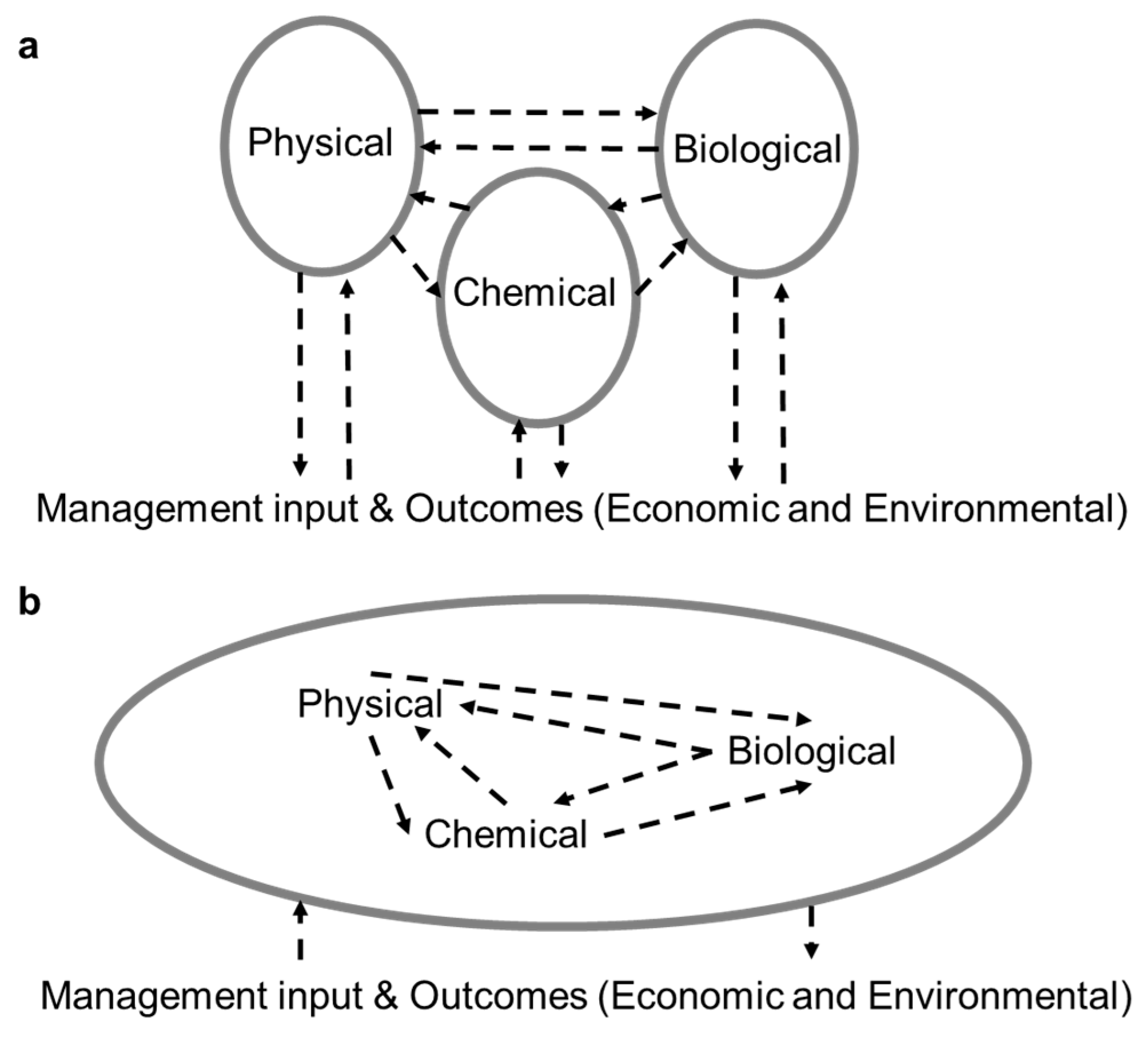
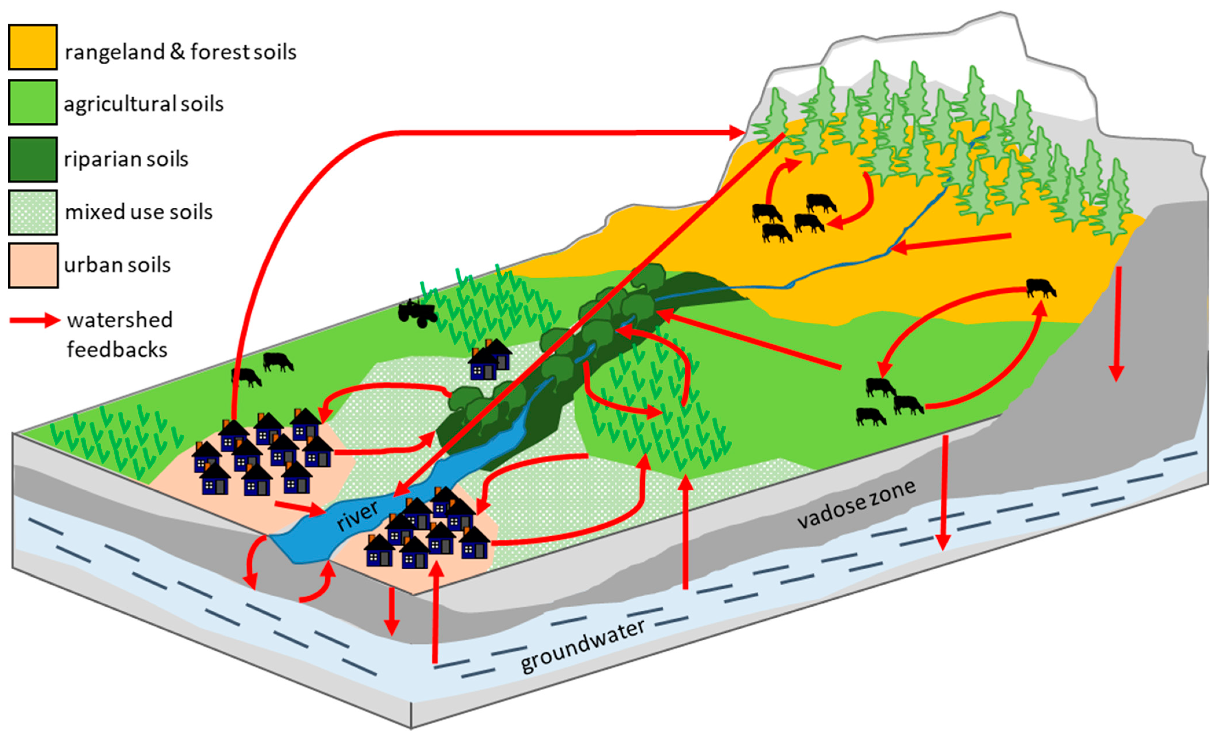
1.1.2. Tightly Coupled

The elements or components within systems strongly interact with one another, human actors, and other parts of the natural world; a feature often summed up in the phrase “everything influences everything else” [14,15,25]. Within soil systems, there exist strong coupling and interaction between soil physical features (porosity, bulk density, etc.), chemical elements (nutrient storage and release), and living microorganisms (organic matter turnover) and plant roots (below ground), as well as with above-ground components such as plant litter, biodiversity, and human decisions about soil and land management [29,30,31,32]. Indeed, changing or manipulating any one of the factors would inevitably lead to changes in everything else.

1.1.3. Governed by Feedback

Because systems are tightly coupled, behaviors tend to feedback on themselves. As changes in conditions take place in one component or over time, the consequences of those changes feedback on other parts of the system, leading to new conditions elsewhere, which in turn feedback to reinforce or offset the original perturbations [14,15,25]. Due to the importance of feedback as a concept as well as in the remainder of this paper, several examples are illustrated and discussed below.

Feedback processes are pervasive in soil systems at a variety of spatial scales. For example, rhizosphere interactions between plant roots and soil food webs are made up of self-reinforcing and self-regulating cycles. For example, positive feedback driven by root exudation, microbe population growth, microbially-induced nutrient release, and plant root nutrient uptake facilitates subsequent root exudation (a self-reinforcing process), while negative feedback driven by predator-prey consumption and initial nutrient availability govern nutrient turnover rates useful for plant growth (self-regulating cycles) (Figure 2 [33,34,35,36]).

Moving from the rhizosphere to the soil column, local biogeochemical cycles emerge as feedback processes (Figure 3). Here, above- and below-ground processes are linked via nutrient cycling from the soil column into terrestrial biomass of plant material through root uptake as well as through soil moisture-mediated evapotranspiration [37,38,39,40,41,42,43,44,45,46]. Plant biomass that is not removed (e.g., crop removal through harvest or grazing animal consumption) is returned to the soil surface as plant litter. Plant litter is the primary input to soil organic matter that eventually is able to supply nutrients back to the plant, made possible by the microbial interactions that feed on organic matter and transform nutrients from plant unavailable to available forms. Inevitably, some nutrients are lost due to biomass removal or erosion and runoff, requiring inputs via N-fixation or fertilization. Organic matter and other nutrients may accumulate or deplete depending on the net rate of these additions, such as photosynthesis, N-fixation or fertilization, or losses, such as biomass removal, leaching or runoff and erosion. Such feedback processes in the soil column allow for nutrient in the balance to be both utilized (by plants) and conserved (minimizing losses to external sinks).

Moving beyond the soil column introduces additional sources of feedback, namely, socio-economic feedback based on human responses to observed or expected soil functions provided by the soil ecosystem via the above rhizosphere and soil column feedback processes. In any case where human decision making is a factor, feedback is at work given the well-established principle that “all decisions take place in the context of feedback-information processes” [47]. For example, the current soil ecosystem may provide a particular crop yield or forage grazing potential, which contributes to the expected payoff of the farmer or land owner (Figure 4). If this payoff does not meet expectations, pressure is felt to alter management conditions, for example, reducing crop diversity to focus on highest valued crop, increasing livestock numbers to achieve a larger herd capable of greater sales, exploring alternative biomass markets which may lead to reduced crop residues as more is harvested or utilized, among other options. By altering these management conditions, cascading feedback effects occur to a range of soil processes: fewer nutrients returned to the soil surface and greater tillage requirements deplete organic matter; greater use compacts soil pore spaces, leading to reduced water infiltration and soil site stability, which accelerates erosion. These soil qualities directly impact the soil ecosystem, which in turn feeds back to the observed outcomes, prompting management responses (i.e., yield, grazing, and expected payoff; Figure 4). Although this example is one of cascading feedback that reduces soil ecosystem functions, the reverse case is also true. Improving soil processes can lead to synergistic improvements throughout the soil ecosystem that reinforce conservation efforts and farmer payoffs (e.g., conservation agriculture).

Feedback processes also exist at the watershed scale that link people, land use, and soil processes in ways that interact spatially across the landscape, linking geography, topography, soil limitations, potential and actual land uses, urban soils and population centers (Figure 5). Communities utilize ecosystem goods and services from upland rangeland and forest soils, riparian and valley soils, agricultural soils, and water runoff in order to sustain themselves. In doing so, they influence the health and function of the respective soil systems via enacted management and policy aimed at promoting benefits they expect to receive in the urban or residential areas [48,49,50,51,52]. In addition, internal feedbacks exist within each type of soil system (including but not limited to those in Figure 2, Figure 3 and Figure 4) and feedback exists between upland, lowland or riparian, agricultural, and urban soils and with below-ground resources and processes, such as the vadose zone and groundwater reserves [53,54,55,56,57].

1.1.4. Nonlinear

Nonlinearity describes the nonproportional relationship between effects and their causes and the nonuniform propagation of cause and effect through space. In socio-economic systems, such nonlinear outcomes have been observed in supply chain inventory management, where a small inventory shortfall leads to overcorrections in production, which inflates inventory for long periods of time because production can never fall below zero (e.g., a phenomenon commonly referred to as the Forrester or bullwhip effect) [17,58]. Nonlinearity effects of these kinds are observed in soils in a myriad way: soil moisture-mediated evapotranspiration takes on multiple linear and exponential forms [38,39,40,41]; nonuniform water infiltration–excess runoff patterns in response to precipitation forcing; exponential salt accumulation in soil during irrigation appears negligible at first until levels begin limiting evapotranspiration [43]; improvements in soil function with conservation adoption appears slow at first (<3–5 years) before significant measurable improvements may be seen, while soil degradation may occur with one extreme natural (e.g., flood or drought) or anthropogenic event (e.g., moldboard plowing); cultivation may continue for decades with only gradual soil loss that eventually depletes the topsoil at once and jeopardizing remaining soil capacity [8,9,27,28].

1.1.5. History Dependent

The behaviors of complex system are path dependent (i.e., potential chains of cause and effect over time are mutually exclusive) and irreversible (i.e., given the second law of thermodynamics) [14,15,25]. One does not need to look far for this principle in soil systems, and importantly, one of the most significant contributions in soil science, Hans Jenny’s The Factors of Soil Formation [59]. Jenny’s Factors include the factor of time, which was perhaps the first recognition that variability is, in part, a function of how a particular soil develops over time (i.e., different influences and time scales equate to unique path dependencies). History dependence is also a critical feature in soil recovery and conservation efforts, as previous disturbances to a soil, such as cultivation, overgrazing, or mining, often have long-term impacts on the structure and function of that soil, a concept called a legacy effect [9,60]. A soil legacy is the influence that previous land or soil use activities have on current ecosystem structure and function long after those activities have ceased (i.e., a time-delayed or unintended impact, potentially either positive or negative) including loss of soil and/or changes in soil properties [4,61,62,63].

1.1.6. Self-Organizing

Dynamic behaviors are the result of a system’s internal structure, which can either dampen or amplify random shocks over space and time [14,15,25]. Ecology has long recognized self-organization in ecosystem perspectives grounded in the structure-based and function or behavior-based perspectives [64], which state that the organization of biotic and abiotic elements and the distribution of energy in the ecosystem (i.e., the structure) drives trophic-level interactions, nutrient cycling and storage, ecosystem processes, and adaptation to disturbances (i.e., the behaviors). In socio-economic systems, markets arise spontaneously from feedbacks between agents [14,15]. With regard to soil systems, Hans Jenny’s insights into soil formation again bears on soil system dynamics. Besides time, Jenny recognized that unique soil pedons are the result of feedbacks between parent material, organisms, climate, and relief, operating simultaneously (i.e., self-organizing) to produce diverse soil types.

1.1.7. Adaptive

The capabilities and rules (i.e., of decisions, policies or strategies, and management) change over time as adaptations take place to learn from experience, exploit environmental conditions, and hedge against risk (both economic and biologic). Although adaptions based on the above factors are meant to find new ways to achieve particular goals (profit, survival, etc.), not all learning is beneficial if feedback is misinterpreted and leads to reinforcing poor decision making [14,15,17,19]. Ecosystems also express adaptive qualities that allow for change and evolution in their internal structures in order to better cope with external stressors (e.g., mutations and allostasis, phenotypic plasticity, migration and habitat selection, redundancy and response diversity, among others, [64,65]). Because of the high degree of feedback processes at which soil lay at the center (Figure 2, Figure 3, Figure 4 and Figure 5), soils systems are able to adapt and respond to changing conditions, such as shifts in soil microbial community composition, plant–soil feedbacks that condition soil physical and chemical properties as well as plant species diversity and health and soil aggregate formation or dissipation processes [30,31,66]. Soil adaptive capacity is especially evident where management is concerned-soils may rapidly adapt to changes in management (e.g., aggregation, soil water infiltration, and nutrient availability) or resist change due to inherent soil properties that force management to accommodate these features (e.g., pH, salinity, and soil depth limitations).

1.1.8. Exhibit Trade-Offs

Long-term results often differ from short-term outcomes due to time delays embedded in the system’s feedback structure [14,15,25]. Low-leverage interventions often lead to better-before-worse behaviors, misleading observers in the short turn to associate improved behaviors with less than reliable interventions. On the other hand, high-leverage interventions to a system often lead to worse-before-better behaviors, which can mislead observers to associate failed responses with the intervention that was in fact the more sustainable one. Managing soil systems poses such trade-offs. For example, in many places throughout the world, adoption of conservation agriculture practices, many of which are known to conserve soil, water, and nutrients, improve soil processes such as nutrient cycling, and enhance long-term economic returns, has stalled [67,68,69,70]. Unfortunately, the benefits of such practices are not realized instantaneously, so the short-term reduction in soil function, agricultural productivity, and economic returns [71,72,73] experienced during the soil rehabilitation process often leads managers to “abandon” practices prematurely. It is not uncommon for the full benefits of conservation practices to be realized 5–10 years (no-till only) or 40–60 years (no-till + diverse crop rotations) after implementation [74,75].

1.1.9. Counterintuitive

Cause and effect are distant in time and space yet we look for causes near the events we seek to explain [14,15,25]. The counterintuitive principle (along with policy resistance, described below) captures the human dimensions involved in observing, understanding, and responding to the behavior of soil systems and the processes and outcomes directly attributable to human use or environmental stresses. To illustrate the counterintuitive principle observed for soil systems, we may consider both a historical and contemporary example.

During the Dust Bowl era in the United States, the causes of significant erosion were ascribed to the then on-going drought of the western Great Plains (although true, this explanation does not tell the whole story). The causes that led to the Dust Bowl actually began decades earlier through several factors: (a) westward explanation was incentivized by the United States government, who offered land to homesteaders willing to settle the frontier and farm to support themselves, leading to conversion of millions of acres from perennial grasslands to cultivated agriculture; (b) reliance on moldboard plowing (the primary soil cultivation method) that inverted the soil surface layers, exposing bare ground and destroying soil aggregates; and (c) the belief of both policy makers and farmers, grounded in the experience of agricultural expansion on the eastern coast, that sustained cultivation in the west was possible since favorable climate followed cultivation (i.e., that there would be few climate or inherent soil limitations to farming) [76]. Decades of these forces, grounded in assumptions made in climates hundreds of miles away and temporally separated by decades from the Dust Bowl years, led to the conditions of degraded soil surfaces that, once combined with drought, led to the infamous Dust Bowl period.

In more recent times, soil with perennial grassland cover has been converted at alarming rates to cultivation in response to increased demand for biofuels beginning in the mid-2000s and this conversion has driven significant erosion events [8,77]. This sharp escalation in demand was supported by public policy (e.g., the Renewable Fuels Standard), which aimed to increase the supply of alternative energy sources, thereby reducing energy prices (which were rising in response to continued conflict in the Middle East stressing oil supply lines). Although many conservationists and environmentalists blamed farmers for the land conversion and subsequent rapid rise in erosion incidents, the causes and incentives began much farther away, in Washington DC and around the world.

1.1.10. Policy or Management Resistant

Finally, the principle of policy resistance states that the complexity of systems (arising from the internal structure, feedback processes and system characteristics described above) overwhelm our ability to property intuit their structures and behaviors [14,15,25]. Put simply, human intuition breaks down in the face of complexity even with only a small number of variables (<3–5 variables) and often leads us to use heuristics (or decision “short cuts”) when responding to change, which can result in sub-optimal decisions [18,78,79]. Resistance to policy and management changes has been observed in other natural resource systems: flood control efforts that have led to more severe floods, forest fire suppression that has led to more severe fires, and water regulations that have not curtailed the depletion of groundwater stocks.

As we have seen, soil systems are just as complex as (if not more complex than) these other systems, made up of biological, chemical, and physical properties (numbering in the order of dozens of factors) interconnected through numerous feedback processes and operating at various temporal and spatial scales. Because of this, many obvious solutions to soil-related problems often fail or make problems worse:

• Fertilization overcomes soil nutrient deficiencies by providing nutrients in plant-available form, but artificially high resource conditions shift microbial community structure and activity away from guilds specializing in decomposition of organic compounds or potential synergistic plant root–microorganism symbioses; under reduced nutrient cycling, plant production increasingly relies on fertilization to meet nutrient needs at the field scale [36,80,81,82] and can contribute nutrient-driven externalities at larger scales.
• Irrigation overcomes soil moisture deficiencies that limit plant transpiration but often introduces salts and other chemicals into the rooting zone that accumulate over time with subsequent irrigation events (especially in situations with poor drainage and water quality, an effect known as secondary salinization). Eventually, the accumulated salts limit plant transpiration, trading one problem (soil moisture availability) for a more challenging one (salt accumulation) [43,83,84,85,86,87,88].
• Tillage provides beneficial results by opening soil pore spaces, breaking up compacted layers, and accelerating nutrient release. However, continued tillage eventually destroys soil aggregates by decoupling soil aggregation processes, reducing pore space and increasing bulk density, which in turn minimizes microbial community habitat and nutrient capture and release. This biophysical trade-off alters nutrient management in the short term [89]; and in the long run, such degradation processes have contributed to the growth and collapse of societies [90].
• Biochar has increasingly been suggested as an amendment to accelerate soil carbon storage. However, short-term carbon emissions often increase after biochar application and other management factors may override benefits of biochar to improving soil functions (e.g., more difficult weed control, introduction of contaminants, microbial community shifts, and rapid pH change) [91].

Based on the above principles and their evidence, it is argued that soil is an archetype of a complex system. Recognizing this reveals additional progress that must be made across disciplines and applied to soil systems: on the one hand, we need to better understand the structure and behaviors of complex soil systems; on the other hand, our innate ability to comprehend and intuit the structures and behaviors of complex systems remains poor, irrespective of domain expertise or level of education [17,19]. Understanding complex systems requires developing a theoretical foundation from which to study ecological, biophysical, and socio-economic processes at various scales and test predictions against observations.

Dynamic simulation modeling, at the systems level, provides such a theoretical foundation and complements reductionist laboratory and field experiments given treatments can be examined without space, time, or cost limitations or uncontrolled variability in system parameters [91,92]. Through simulation modeling, the outcomes and consequences of different ecosystem properties, land uses, input levels, climate, and importantly, management decisions can be analyzed and assessed. Using models in this way provides a simple and rapid yet robust means for improving our understanding of both anecdotal and experimental data by explicitly accounting for feedback processes across temporal and spatial scales. Because variability among soil units is extremely high it can be difficult to interpret how different interventions will affect soil processes, even in fairly similar soils. Modeling can be an effective laboratory for assessing complex systems and evaluating how management responds to observed conditions and changes in soil system structure and behavior, including in response to varying climate.

To help scientists, managers, and policy makers close this gap between soil system complexity and human intuition (and by doing so be better prepared to respond to environmental externalities related to soil system dynamics, e.g., biogeochemical cycles), a dynamic systems framework is outlined below capturing feedback often excluded from investigation or left to intuition. Then, several simulation case studies are analyzed to illustrate how such a framework can be applied to agroecosystem management problems related to nutrient cycling (e.g., soil water, nitrogen, carbon, and sodium) and common soil-related environmental externalities (e.g., nitrogen leaching, soil salinization). The model and case studies are described below followed by the results and discussion, with particular focus given to the necessity to account for feedback processes to better understand and appreciate the complexity of soil systems and their interface with management.

2. Materials and Methods

2.1. Model Overview

The agroecosystem model integrates biophysical, chemical, and economic decision-making interrelationships that influence the inflows and outflows of water, nutrients, organic matter, and crop yields over time across a soil–water–nutrient–plant continuum. The model was developed from several independent soil models previously documented and peer-reviewed elsewhere [37,38,39,40,93,94,95]. Although no new soil equations are presented here, the approach is novel given the model integrated previously fragmented approaches into a single, cohesive application. The model structure links soil moisture, S (percentage of field capacity), crop production, C (soil surface cover), nitrogen, N, and sodium, Na, balances (with their respective influences on S and C), soil organic matter (SOM), dynamic soil physical properties such as porosity and hydraulic conductivity, and decision factors for fertilization, irrigation, and tillage management. All acronyms used here and throughout the text appear from previous modeling conventions [37,38,39,40,93,94,95]. Dynamic interactions result from the numerous feedbacks as previously illustrated (similar to Figure 3) in a holistic model boundary (Figure 1b). For example, N levels drive C growth, which in turn reduces S, which in turn drives irrigation decisions that may raise Na concentration and slow C growth; C residue provides litter input to SOM stocks, which improve porosity and S storage, reinforcing C growth, while removing C through excessive biomass harvest reduces litter and therefore SOM. The model includes key processes pertinent to each state variable defined above: infiltration–excess runoff dynamics, dynamic evapotranspiration rates (ET; regulated by S), nitrogen turnover and leaching (influencing fertilization decisions and environmental quality), SOM accumulation or degradation, soil physical characteristics (e.g., porosity), and irrigation, fertilization, and tillage decisions (e.g., frequency and depth of irrigation in response to S shortage or fertilization in response to N shortage). Model inputs include climate parameters required to determine reference ET and estimate expected soil temperature as well as precipitation data, while the primary biophysical output, crop yield, feeds back to the economic decision-making considerations which adjusts subsequent input strategies (although all variables can be exported for analysis). The model was constructed in the Vensim™ modeling environment (Ventana Systems, Inc.; Cambridge, MA, USA), a system dynamics (SD) icon-based simulation application, with a time unit was 1 day (time step = 0.25). The SD environment is especially useful for simulation involving hundreds of coupled feedback processes. In the sections below, a description of key feedback components is provided, but because the model and its components have been presented previously [37,38,39,40,93,94,95] only high-level feedback equations are shown for simplicity. We then describe the case study simulations tested to evaluate the outcomes of several pressing agroecosystem management problems.

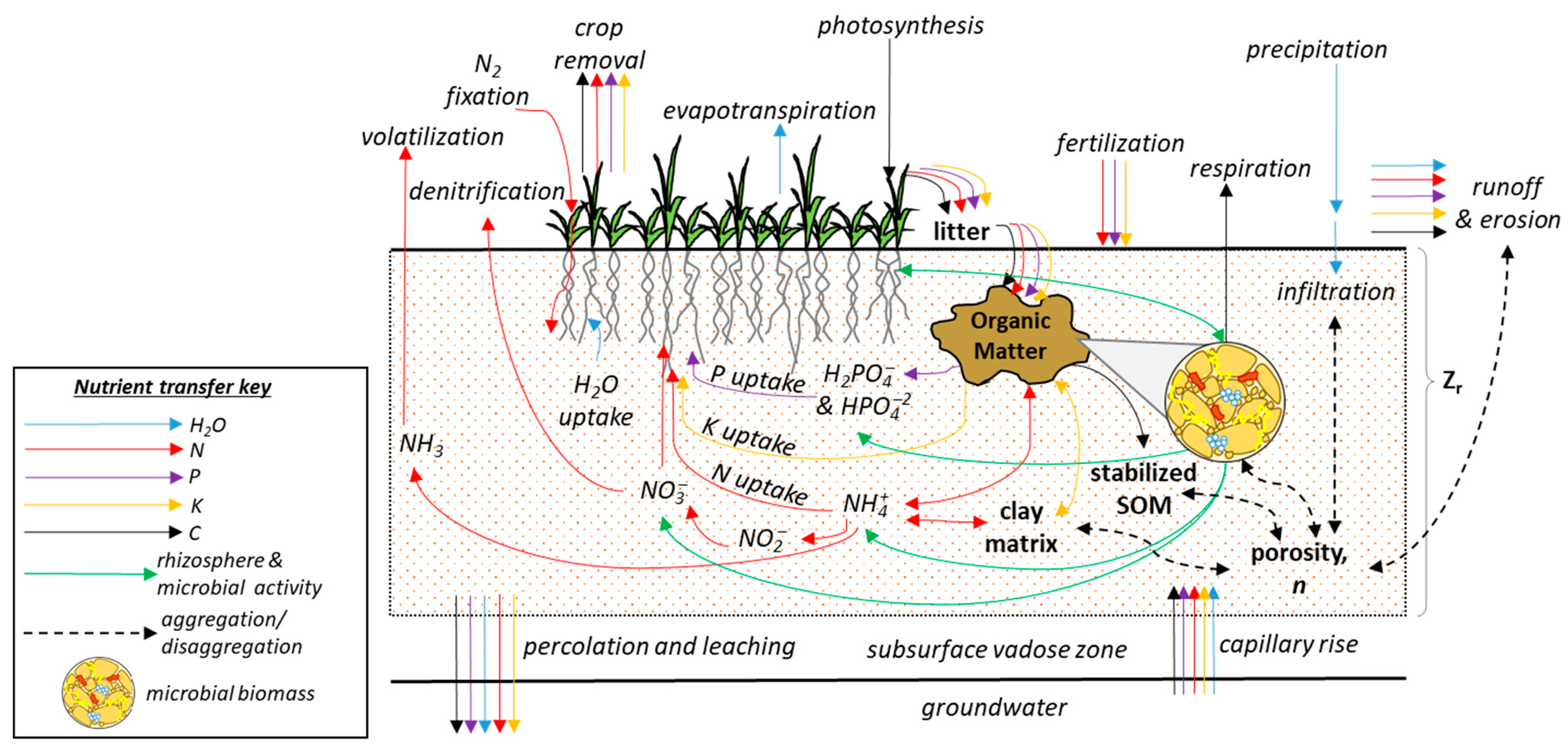
2.2. Model Nutrient and Chemical Components

The core physical equations are provided in

Table 1. Summary list of model physical/chemical equations constituting the core structure of the agroecosystem model, developed from [37,38,39,40]. * Descriptions indicate operationalized feedback linkage with other model components.

Equation	Equation No.	Soil Nutrient/Chemical Component
nZr (dS/dt) = R(t) + I(S(t)) − ET(S(t), C(t)) − Q(S(t))	(1)	Water balance *
ET(S(t), C(t)) = ETs * C(t) * Kcb * ET0	(2)	Total ET
${\mathrm{ET}}_{\mathrm{s}}=\{\begin{array}{cc}{\mathrm{ET}}_{\mathrm{w}}\frac{\mathrm{s}-{\mathrm{s}}_{\mathrm{h}}}{{\mathrm{s}}_{\mathrm{w}}-{\mathrm{s}}_{\mathrm{h}}},& {\mathrm{s}}_{\mathrm{h}}<\mathrm{s}\le {\mathrm{s}}_{\mathrm{w}},\hfill \\ {\mathrm{ET}}_{\mathrm{w}}{+(\mathrm{ET}}_0-{\mathrm{ET}}_{\mathrm{w}})\frac{\mathrm{s}-{\mathrm{s}}_{\mathrm{w}}}{{\mathrm{s}}^{\ast }-{\mathrm{s}}_{\mathrm{w}}},& {\mathrm{s}}_{\mathrm{w}}<\mathrm{s}\le {\mathrm{s}}^{\ast },\hfill \\ {\mathrm{ET}}_0,& {\mathrm{s}}^{\ast }<\mathrm{s}\le 1.\hfill \end{array}$	(3)	Soil moisture-regulated transpiration
E(S, C, t) = Kr(S) * (1 − C) * Eb * ET0(t)	(4)	Evaporation driven by soil cover
$\mathrm{Kr}\left(\mathrm{S}\right)=\{\begin{array}{cc}0& \mathrm{s}\le {\mathrm{s}}_{\mathrm{h}}\hfill \\ \frac{\mathrm{s}-{\mathrm{s}}_{\mathrm{h}}}{1-{\mathrm{s}}_{\mathrm{h}}}& \mathrm{s}\ge {\mathrm{s}}_{\mathrm{h}}\hfill \end{array}$	(5)	Evaporation reduction coefficient
K(S) = Ksat * Sd	(6)	Hydraulic conductivity
dC/dt = G(C, S, N, t) − −Ms(C, t) − H(C, t)	(7)	Plant canopy cover
G(C, S, N, t) = rg * U(C, S, N, t)	(8)	Plant growth rate
Ms(C, t) = (rm + γ (t − tsen) * Θ (t − tsen)) * C2	(9)	Plant senescence
Hi = C * Hv * Hd	(10)	Plant harvest
dNc/dt = D(C, t) + F(N, t) − L(S, N) − U(S, N, C, t)	(11)	Nitrogen balance *
L(S, N) = η * Q(S)	(12)	Nitrogen leaching
η = aN/SnZ	(13)	Soil water nitrogen content
U(S, N, C, t) = f(η) * T(S, C, t)	(14)	Plant nitrogen uptake
$\mathrm{f}\left(\mathsf{\eta }\right)=\{\begin{array}{cc}\frac{aN}{SnZ}& \frac{aN}{SnZ}<\mathsf{\eta }\mathrm{c}\hfill \\ \mathsf{\eta }\mathrm{c}& \frac{aN}{SnZ}\ge \mathsf{\eta }\mathrm{c}\hfill \end{array}$	(15)	Nitrogen uptake limitation function
dqs/dt = IVi – Q * V	(16)	Soil salinity
dB/dt = W * U(S, N, C, t)/ηcET0(t) = W/ηc Ks(S)Kcbf(η)C	(17)	Crop biomass
Y = B * Hi	(18)	Crop yield *
$\mathrm{IE}=\frac{{{\displaystyle \sum }}_{\mathrm{t}=0}^{\mathrm{t}=\mathrm{final}\mathrm{time}}\mathrm{transpiration}}{{{\displaystyle \sum }}_{\mathrm{t}=0}^{\mathrm{t}=\mathrm{final}\mathrm{time}}\mathrm{I}\left(\mathrm{S}\right(\mathrm{t}\left)\right)}\ast \mathrm{irrigation}\mathrm{fraction}\mathrm{of}\mathrm{total}\mathrm{water}\mathrm{inflows}$	(19)	Irrigation efficiency
$\mathrm{NUE}=\frac{{{\displaystyle \sum }}_{\mathrm{t}=0}^{\mathrm{t}=\mathrm{final}\mathrm{time}}\mathrm{U}}{{{\displaystyle \sum }}_{\mathrm{t}=0}^{\mathrm{t}=\mathrm{final}\mathrm{time}}\mathrm{F}}$	(20)	Nitrogen use efficiency

with definitions for each parameter and related source material in Appendix A. The soil-water (S) balance (Equation (1)) is a function of precipitation, R, irrigation, I, evapotranspiration, ET, and leakage, Q. Evapotranspiration (ET; Equation (2)) is a dynamic flux dependent on estimated transpiration, which is regulated by S (Equations (3) and (5)), as well as plant canopy cover, C (Equation (4)). Leakage from the soil column is primarily a function of hydraulic conductivity (Equation (6)).

Plant canopy cover, C, grows as a function of current photosynthetic potential (i.e., current C), soil moisture S, nitrogen N, and time, t, and is reduced through senescence, M, and harvest, H (Equation (7)). Plant growth, G, is a function of nutrient uptake, U, itself driven by available S, N, and demand from existing C and a scaling constant, r_g, for amount of plant cover added per unit of nitrogen utilized (Equation (8)). Plant senescence, M, takes on a nonlinear (exponential) function of canopy C based on estimated time of senescence, t_sen (Equation (9)), while harvest is a point in time removal of canopy at harvest time, H_d, and harvest volume, H_v (Equation (10)).

The nitrogen balance (Equation (11)) is a function of natural deposition, D [which is provided to the soil via canopy turnover to SOM (1 − H_v)], fertilization, F, leaching, L [Equation (12), driven by fluxes in S represented by leakage Q and water nitrogen content, η (Equation (13))], and plant uptake, U, given as the amount of nitrogen absorbed during transpiration, T (Equation (14)), which is limited by a saturation function to insure that nitrogen uptake does not exceed biologically realistic values (Equation (15)).

Salinity, q_s, is given by the amount of irrigation applied, I, and the salt concentration in irrigation water, V_i, and any leakage of salts through Q (Equation (16)).

Plant canopy cover is converted to crop biomass, B, using a conversion function (Equation (17)), where W represents a productivity index of biomass produced given the efficiency of nutrient uptake (Equation (17)). Yield is simply B multiplied by the harvest index, h_i, the fraction of harvested plant cover, H_v, that is converted to marketable yield (Equation (18)).

Irrigation efficiency, IE, is estimated by the ratio of transpired to applied water and adjusted for irrigation fraction of total water received (irrigation + precipitation) (Equation (19)), while nitrogen use efficiency, NUE, is measured by the nitrogen volume taken up by the plant relative to the total nitrogen applied through fertilization (Equation (20)).

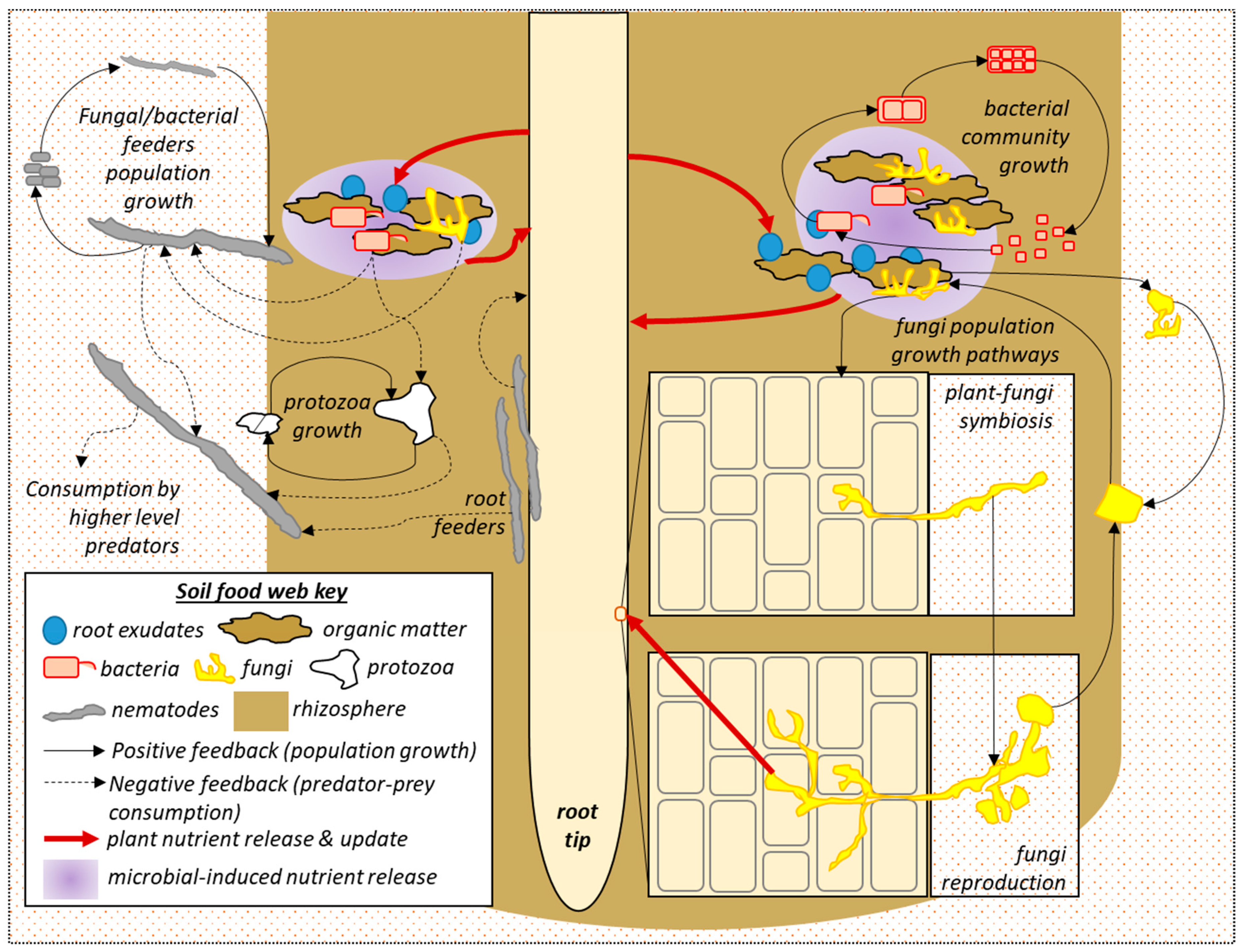
2.3. Model Biological Components

The model’s biological component includes feedback processes for organic matter turnover (from canopy cover, C, to soil litter, to soil organic matter, SOM, to soil N to N uptake, back to C) as well as organic matter influences on soil porosity and infiltration (based on SOM dynamics replicated from [93,94,95]). The core biological equations are provided in

Table 2. Summary list of model biological equations constituting the core structure of the agroecosystem model, developed from [93,94,95]. * Descriptions indicate operationalized feedback linkage with other model components.

Equation	Equation No.	Soil Biology Component
dSOMi/dt = Ki * Md * Td * SOMi	(21)	Organic matter dynamics
${\mathrm{M}}_{\mathrm{d}}=\{\begin{array}{cc}1/(1+30\ast \mathrm{e}^(-8.5\ast \mathrm{RAT}\left)\right)\hfill & \mathrm{RAT}>1.5\hfill \\ 1-0.7\ast \left(RAT-1.5\right)/1.5\hfill & \mathrm{RAT}\le 1.5\hfill \end{array}$	(22)	Soil moisture effect on decomposition rate
Td = (t1 * 0.2) * t2	(23)	Soil temperature effect on decomposition rate
Ki1 = K1 * exp (−3.0 * Lf)	(24)	Litter layer decomposition rate
Ki5 = K5 * (1 − 0.75 * (silt + clay fraction))	(25)	Soil texture effect on active carbon decomposition *
Lfa = 2 + 0.12 * PPT; where PPT is the annual precipitation	(26)	Precipitation effect on above-ground lignin biomass
Lfr = 26 − 0.15 * PPT; where PPT is the annual precipitation	(27)	Precipitation effect on root lignin biomass
Fm = 0.85 − 0.018 * LR/N	(28)	Residue microbial metabolic supply *
Fs = 1 − Fm	(29)	Residue structural component
SOMslow = (0.85 − 0.68 * (silt + clay fraction))	(30)	Soil texture effect on stabilizing slow SOM *
RAT = (S(t) + R(t))/ET0	(31)	Md inputs *
temp1 = (45 − ts)/(45 − 35); temp2 = e^(0.076 * (1 − temp1 * 2.63)); where ts is temperature degrees °C	(32)	Td inputs

with definitions for each parameter and related source material in Appendix A. The soil organic matter (SOM_i) balance (Equation (21)) is a function of maximum possible decomposition rate (K_i), regulated by the effect of moisture (M_d, Equation (22)) and temperature (T_d, Equation (23)) for i states of SOM: surface and soil litter and active, passive, and slow soil carbon stocks. The SOM component’s carbon cycle includes flows from surface and soil litter to active and slow soil carbon, and coupled flows from active soil carbon with slow and passive stocks, as well as respiration losses from each stock that accompany carbon transfers (conceptualized and described in [93,94,95]).

Decomposition rate K_i is constant except for surface layer litter decomposition rates (Equation (24)) and active soil carbon (Equation (25)). Litter decomposition (K_i1) is a function of the lignin content (fraction) of above-ground litter, Lf_a (Equation (26)) and root biomass, Lf_r (Equation (27)), with the lignin fraction being driven by changes in annual precipitation (PPT), while active soil carbon respiration (K_i5) is primarily regulated by soil texture (combined silt and clay percentage). Litter is partitioned into structural or metabolic stocks based on the lignin to nitrogen ratio (LR/N) (Equations (28) and (29)). Storage of soil carbon from active into slow pools (turnover times > 25–1000 years) is likewise regulated by texture characteristic (Equation (30)).

Soil moisture effect on decomposition, M_d, is a function of soil moisture (S + R) relative to potential evapotranspiration demand (ET₀) (Equation (31)), while temperature effect, T_d, is an empirically derived equation based on soil temperature (°C) (Equation (32)).

The biological model component, following [93,94,95], assumes that are carbon decomposition flows result from microbial activity and that microbial respiration is associated with all flows between carbon stocks.

2.4. Model Soil Physical and Hydraulic Component

Soil and crop management factors interact to alter soil physical processes and functions. The core physical and hydraulic equations are provided in

Table 3. Summary list of model physical and hydraulic equations constituting the core structure of the agroecosystem model, developed from [44,45,96,97]. * Descriptions indicate operationalized feedback linkage with other model components.

Equation	Equation No.	Soil Physical and Hydraulic Component
dr/dt = d(vf)/dr − mf	(33)	Pore radius distribution
n(t) = a(t)r−b(t)dr	(34)	Soil porosity dynamics *
v(r, t) = r/(a(t)b(t)) * (a(t)b’(t)ln(r) − a’(t))	(35)	Soil particle space drift and shrink term
m(r,t) = b’(t)/b(t) * (1 − ln(r)) − a’(t)/(a(t)b(t))	(36)	Soil particle space source-sink term
ψs (S, t) = −(Cs/Rm(t)) * s−1/(1 − b(t))	(37)	Matric potential
Ksat (s, t) = [(γw * Ge * n(t)2 * Rm(t)2 * (1 − b(t))2]/μ (3 − b(t))(2 − b(t))) * s(4 − 2b(t))/(1 − b(t))	(38)	Saturated conductivity *
γb = rb + (1 − rb) * exp(−kb(ttd))	(39)	Management (tillage) influence on porosity
bc(SOM(t)) = b0 + σbOM(t)	(40)	Soil organic matter influence on porosity
b(ttd, SOM(t)) = γb * bc	(41)	Combined b-term for management and SOM effect on porosity *

with definitions for each parameter and related source material in Appendix A. These dynamics are modeled as changes in porosity, n, and matric potential, ψ_s, based on [44,96]. Pore size distribution, f, is a function of pore radius, r, (Equation (33)), where v is a soil drift/shrink term and m is a source-sink term. Integration of pore size distribution over r yields porosity, n, as a power law distribution (Equation (34)) with scaling parameter a and power law exponent b. Pore radii change as a function of v (Equation (35)) and m (Equation (36)); prime notated variables are time-derivative of the given parameter). Matric potential is expressed as a function of surface tension, C_s, and maximum pore radius, Rm(t) (Equation (37)). Hydraulic conductivity, K_sat, is dynamically estimated using specific water weight and viscosity, γ_w and μ, where G_e is equal to 1/8 (Equation (38); assuming the Hagen-Poiseuille equation [44,97]).

Importantly, the power law exponent b is decomposed into time-dependent variables that capture management influences (e.g., tillage) and consolidation or degradation of soil organic matter (SOM) [44]. For example, alternative tillage practices redistribute soil particles in greater or less degrees away from uniform pore distribution, which is described by an exponential decay function towards the untilled soil pore distribution, expressed as the settling term γ_b (Equation (39)), where γ_b is the management factor used in the b term, r_b is the ratio of the parameter value in an untilled state to the base value, k_b is the rate of settling, and ttd is the time since last tillage event in days (in cultivated agricultural systems, tillage resets the soil pore distribution in the short run). Change in SOM (described above) is treated independently via its own effect on the b term (Equation (40)) where b_c is the parameter value at OM equal to 0 and σ_b is the slope of the b–OM relationship [44]. Assuming a linear relationship provides a simple mechanism to feed back SOM on to soil physical properties. Trade-offs from assuming a nonlinear relationship are described in the literature [44]. The b term is then modeled as the influence of both management and SOM dynamics (Equation (41)). Changes in porosity n over time feeds back to nutrient and biological components, described above.

2.5. Model Economic and Decision-Making Component

The economic component links the outcomes from the above model components with financial information needed to estimate economic feasibility (profit/loss) and inform and update decision making (described below). The economics component accrues input costs and revenues from yield (Equation (18)). Costs include fertilizer expense, driven by unit N cost and volume and frequency of fertilization, and irrigation expense, driven by depth and frequency of water applications and fixed costs associated with various irrigation systems (micro/drip, aerial, flood). Inclusion of various management methods allows examination of trade-offs between irrigation methods. Revenues are estimated using a price per unit of crop, P, multiplied by yield. Uniquely, input rate behaviors can evolve over the course of simulation depending on the selected decision-making strategies.

The decision-making component of the model can assume two particular decision strategies: (a) static, in which case the initial values for irrigation, fertilization, tillage (and combinations thereof) are specified at time = 0 and remain constant through the simulation experiment, or (b) dynamic, in which decision making is linked to the chemical, biological, and physical processes described above and where irrigation, fertilization, tillage (and combinations thereof) rates may be raised or lowered in response to the soil system feedback and the decision-making processes specified for the simulation. In the dynamic case, changes in input rates or soil management practices, collectively noted as IN_r, are made incrementally using the same basic formulation:

IN_r = (SC_desired − SC_observed) * IN_fraction/IN_time

(42)

where the gap between desired soil conditions, SC_desired, and observed soil conditions at a particular intervention threshold, SC_observed, is closed according the fraction of the gap applied in the next application (IN_fraction) over the mean application time (IN_time). Two possible decision-making processes may be employed to adjust these parameters in response to soil processes and economic results: intuitive problem solving (IPS) or analytical problem solving (APS) [98,99,100].

The intuitive (IPS) and analytical (APS) approaches describe two significantly different approaches (often called heuristics) to decision making under uncertainty and complexity [18,98]: IPS is a short-term solution-oriented mental model that employs intuitive responses (e.g., temporary fixes, such as “patching up leaky pipes” or “fertilizing/watering the way out of nutrient deficiency”) without consideration of the root-causes or longer-term unintended consequences, whereas APS is a longer-term, problem-oriented mental model that aims to understand and address root causes of problems (e.g., reinvestment in irrigation system infrastructure; crop diversification and minimizing soil disturbances to improve nutrient capture and turnover). These two approaches are increasingly referred to as “system 1” and “system 2” thinking [18]. For the purposes of simulation experiments described below, it was assumed that IPS is the dominant mode of reasoning regarding agroecosystem input and management [17].

2.6. Model Performance Evaluation

The model’s nutrient and chemical components have been successfully replicated and calibrated to a variety of sites representing diverse soils, climates, and management situations and evaluated extensively via a variety of observational, structural (sensitivity), and statistical tests [37,38,39,40,42,43,44,45,46]. The model’s biological component, which has been simplified from [93,94,95], has been replicated and tested in numerous ecosystems and management settings (from grasslands to forests to cultivated cropland) and has been found to produce excellent results compared to both experimental and long-term SOM monitoring data [101,102,103]. Finally, the model’s physical soil component has likewise been previously evaluated [45]. For these reasons, a detailed description of the multitude tests these models have been subject to for model performance evaluation have not been included, but readers are encouraged to see the above references for model evaluation procedures.

2.7. Case Study Applications in Soil System Investigations

To illustrate the utility of complex, feedback-driven modeling for soil systems, two case study applications pertaining to soil nutrient and agroecosystem management are provided here as proofs of concept, both of which have implications for biogeochemical cycles and environmental externalities: (a) flood vs. drip irrigation decisions, and (b) conventional vs. no-tillage adoption decisions. Under both cases, we assume all of the soil physical, chemical, and biological feedbacks are at work and that managerial heuristics (Section 2.5 above) alter input and management strategies in attempts of maximizing economic returns. All model experiments were conducted using parameters representing an experimental agricultural field site characterized by a loam soil (sand, silt, and clay percentages of 39.2, 37.2, and 23.5%, respectively) of 90 cm rooting depth residing in a semi-arid region with mean annual precipitation of 51 cm, mean soil temperature of 22.7 °C, 400 m above sea level. All experimental treatments were compared to a control treatment, described as a long-term equilibrium condition of 2.5% SOM, no change in long-run yearly profitability, and agroecosystem management characterized by an annual crop production system under conventional tillage (336 kg N fertilization per hectare, 35 cm per year applied irrigation water, and mean yield of 1.2 kg per m² per year). The case study treatments described below were analyzed relative to this control treatment over a 10 year period (treatment parameters are provided in

Table 4. Summary of the two simulation experiments indicating assumed parameter (control) and hypotheses (treatments) values: threshold and target soil moisture levels, S, irrigation application frequency, day of year of tillage event, and harvest volume percentage. * Parameters indicate initial values subject to change given heuristic decision adjustments over time.

		Parameter
		Threshold S (% of Field Capacity)	Target S (% of Field Capacity)	Application Freq (days)	Day of Tillage	Harvest Volume (%)
Exp. 1	Control (flood)	0.35	0.45	21	115	0.67
	Drip irrigation	0.35 *	0.45 *	3	115	0.67
Exp. 2	Control (conv. tillage)	0.35	0.45	21	115	0.67
	No-tillage	0.35	0.45	21	n/a	0.34 *

; visual comparison is shown in Figure 6 illustrating how differing management alters feedback processes).

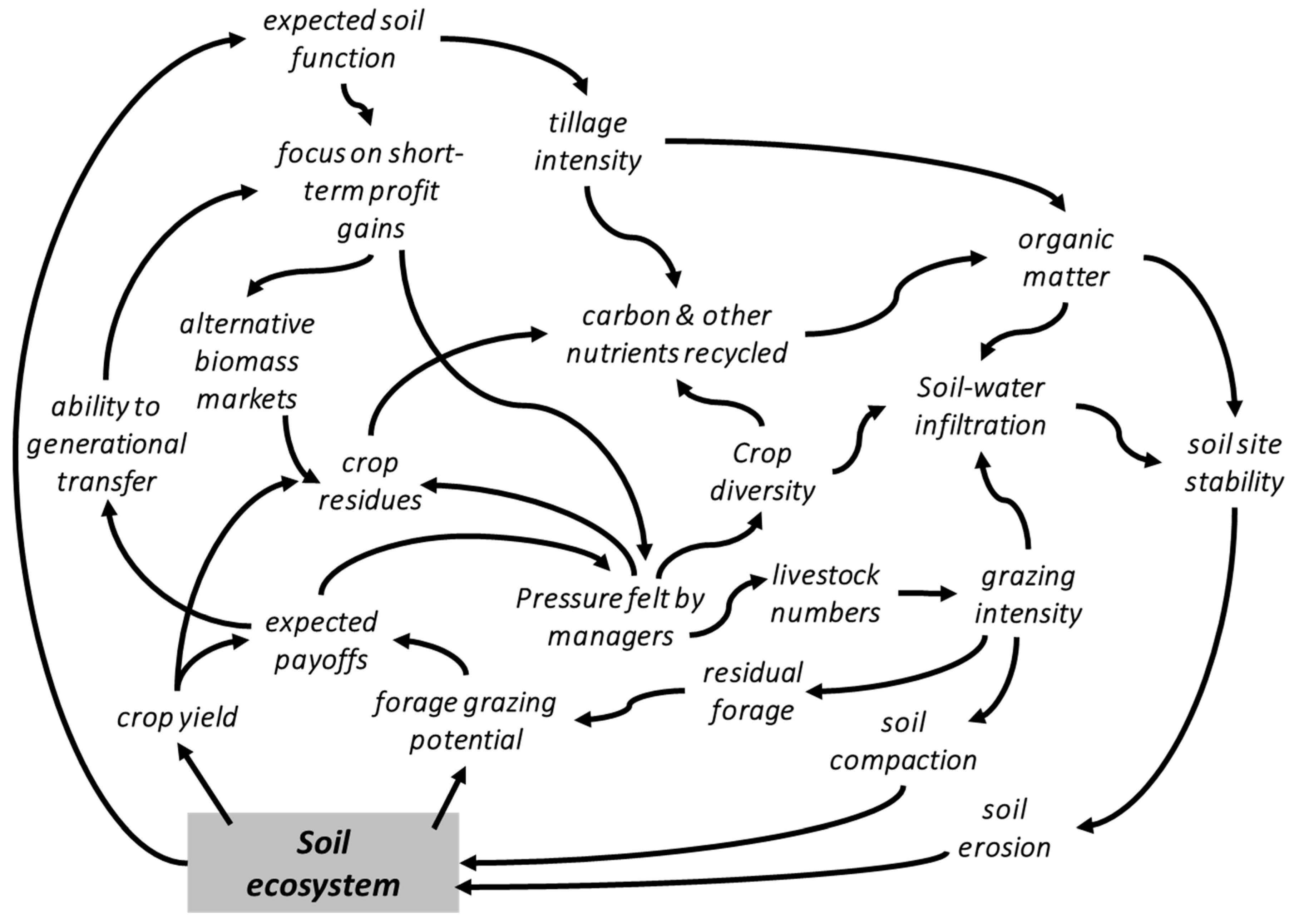
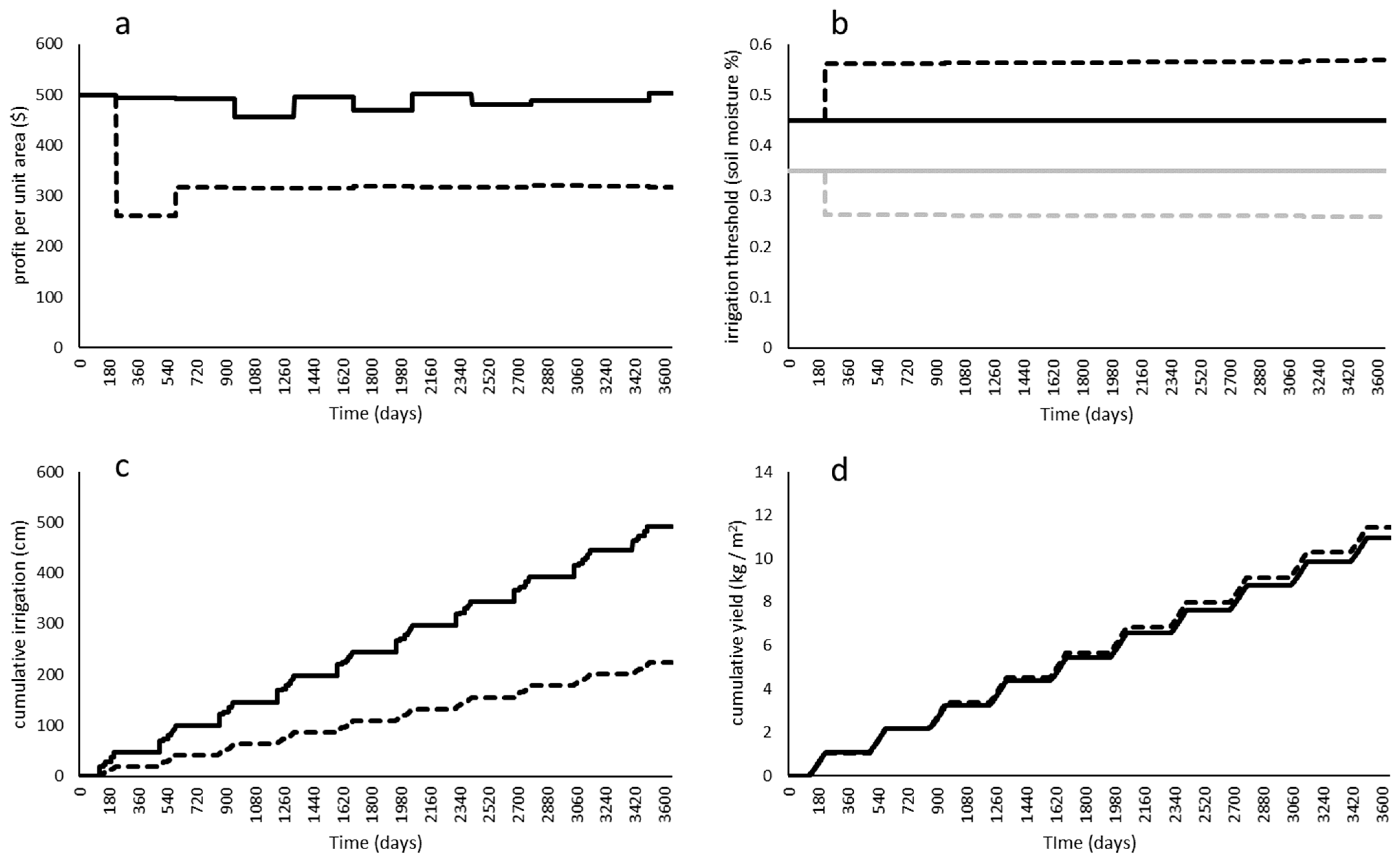
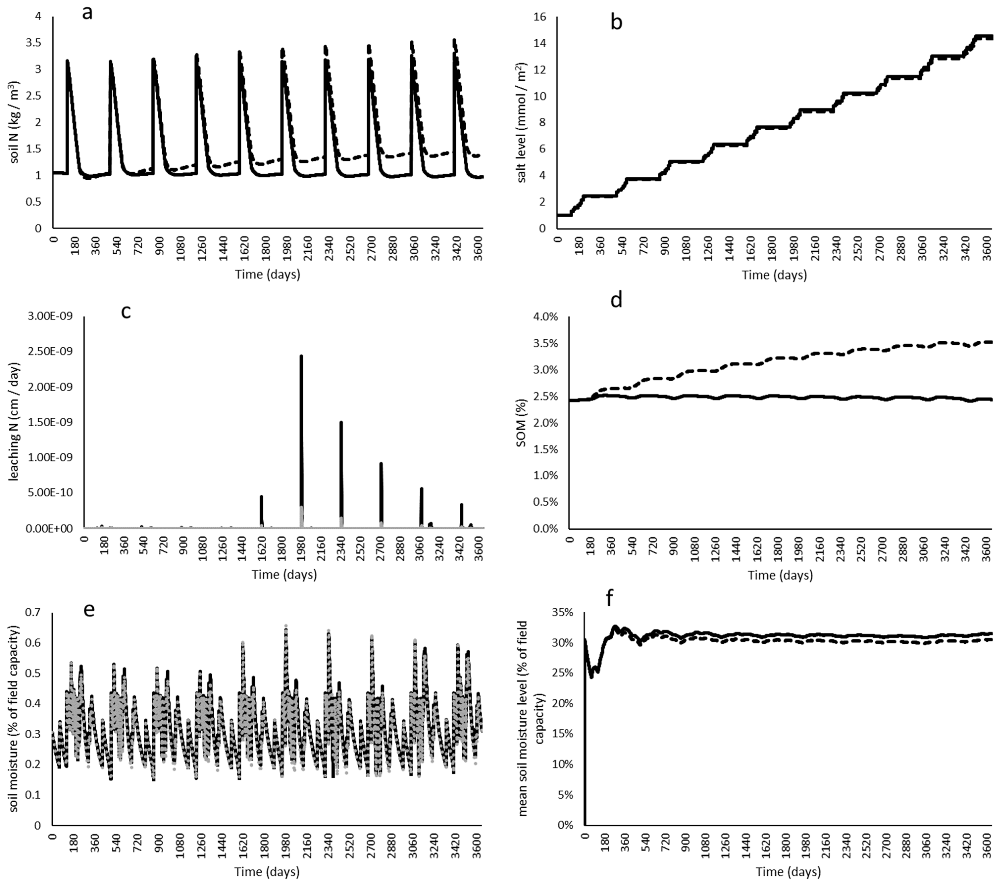
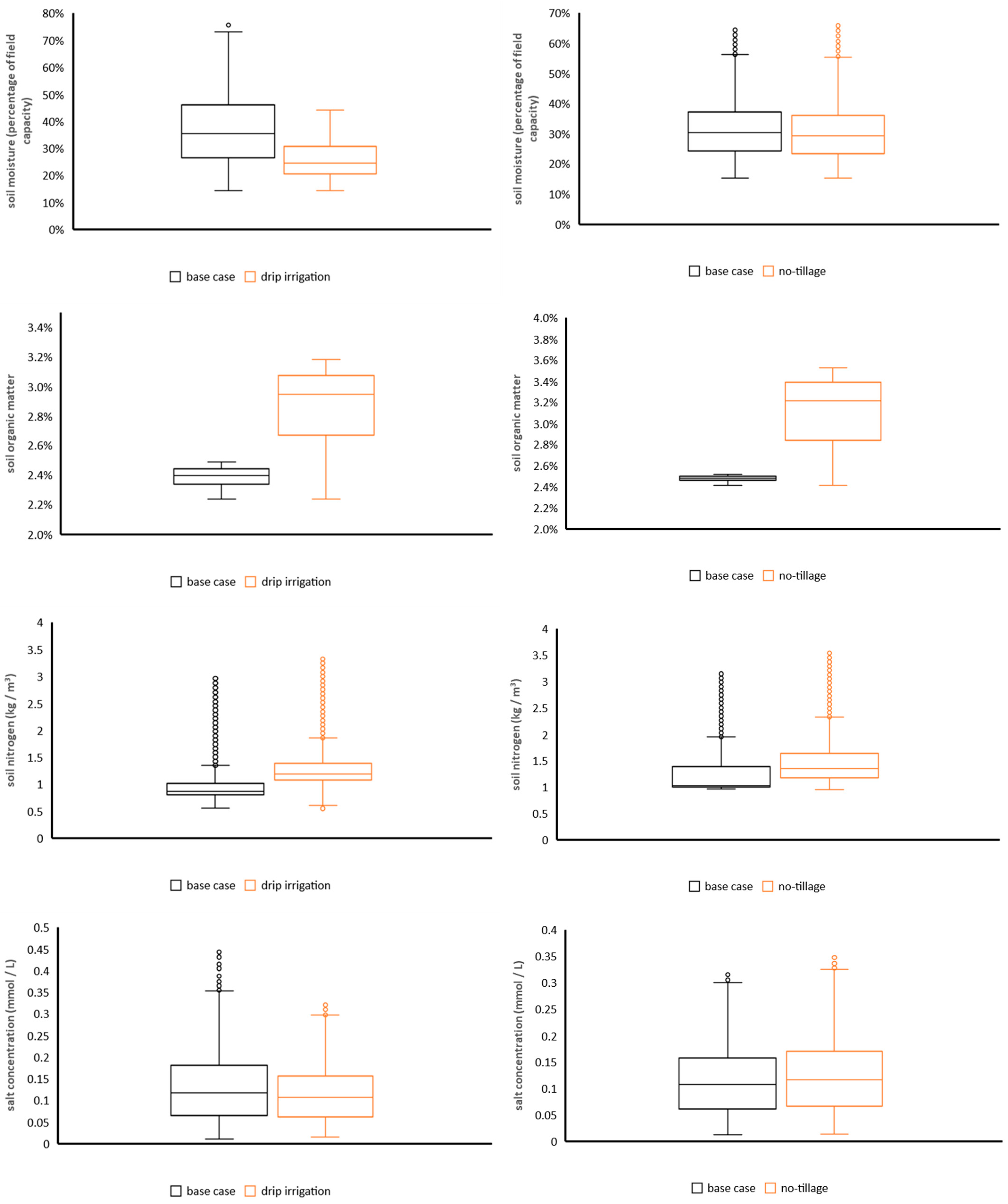
2.7.1. Case Study Experiment 1: Why Do More Agricultural Producers Not Adopt Micro- or Drip Irrigation Systems?

Agricultural water use continues to be the largest freshwater consumer globally, but with increasing populations and domestic water demand, concerns over nutrient loading and water quality degradation, and overall greater awareness as to the need to conserve water of ecosystem health, many agricultural producers have had to develop access to and increasingly rely on new water sources, particularly groundwater. Increasing groundwater withdrawals has precipitated a number of cascading consequences, from increasing salinity, land subsidence, and pumping costs as groundwater levels decline. In addition, irrigation-induced groundwater depletion has a longer-term societal externality given it contributes to overall water scarcity by drawing down available groundwater that in times of stress could be used as emergency water sources, particularly in arid and semi-arid regions experiencing population growth and where shifts in climate (e.g., increasing drought frequency and severity) are already stressing surface water supplies.

Alternative irrigation methods such as micro- or drip irrigation systems are often proposed as high-leverage strategies to minimize the impact of agricultural irrigation on water supplies via the ability to maintain crop production albeit with a fraction of applied irrigation relative to aerial spray or flooding methods, yet adoption of such systems remains low. We therefore test the model to identify causal reasons why such adoption has not taken place via the following hypothesis:

Hypothesis 1a.

Both agroecosystem function and economic outcomes are not significantly influenced by irrigation method (e.g., drip vs. flooding).

Hypothesis 1b.

Both agroecosystem function and economic outcomes will be improved under drip irrigation method relative to flood irrigation.

To implement this test, the conventional (flood) irrigation method was eliminated in favor of a drip irrigation scheme managed using a heuristic based on closing the gap between a threshold soil moisture level that induces irrigation and the subsequent target (desired) soil moisture to meet ET demand—when observed soil moisture reaches the threshold, irrigation is applied until the actual soil moisture reaches the target level. Included in this test are the expected change in fixed costs for added infrastructure, technology, and labor requirements ($250 per unit area relative to $5 per unit area under flooding). If the water savings (in variable cost) and productive gains (in yield) outweigh expected investment in drip irrigation, then we may reject the null hypothesis. In addition, we examine the impact of switching irrigation methods on nitrogen and salt dynamics relative to the control.

2.7.2. Case Study Experiment 2: Why Do More Agricultural Producers Not Adopt No-Tillage Practices in Their Crop Production Systems?

Soil organic matter (SOM) stocks in agricultural soils have declined over the past century due to conventional cultivation and crop management practices [1,104] that leave much of the soil exposed to wind and water erosion and fail to return litter to the soil for decomposition back to organic matter [105,106,107]. These practices include but may not be limited to moldboard plowing pre-planting and post-harvest, monoculture cropping rotated with fallowing or another monocultured cash crop, and heavy doses of nutrient fertilization and pesticides which are detrimental to beneficial soil microbial communities. Besides increased surface layer erosion risk due to destruction of soil aggregates (via tillage) and minimal plant residues to provide protection (via monocropping cash crops without cover or green manure mixtures to return litter to the soil), such practices often are accompanied with a hidden loss of soil function via soil compaction in the subsurface layers resulting from excessive tractor and implement forces at the surface. Although significant at the individual field and watershed levels (as illustrated in Figure 3, Figure 4 and Figure 5), loss of SOM and soil stability have global implications given their importance to biogeochemical cycles, especially carbon and nitrogen, given their importance to climate and environmental health concerns and the level of human alteration already present in these cycles.

No-till agriculture has shown to be highly effective in offsetting these externalities and reversing the trends in SOM and erosion due to the reduction in soil disturbance which leaves aggregates intact and litter in place to protect the soil surface and return as organic matter [108]. Despite these observations, adoption rates of no-till cultivation are still less than might be desired given current soil conditions around the world. We therefore test the model to identify causal reasons why such adoption has not taken place via the following hypothesis:

Hypothesis 2a.

Both agroecosystem function and economic outcomes are not significantly influenced by tillage method.

Hypothesis 2b.

Both agroecosystem function and economic outcomes will be improved under no-till relative to conventional tillage.

To implement this test, the annual tillage treatment was removed with implementation of no-tillage. Under this scenario, it was assumed that harvest volume (Equation (10), the percentage of biomass removed during harvest) is reduced from two-thirds to one-third, or only the yield fraction of above-ground biomass (allowing for greater litter turnover) and that irrigation is provided via aerial spray (both control and treatment given the problem of transporting litter off-site under flood irrigation). The heuristic at work allows the harvest volume, h_i, to vary in response to economic pressure (i.e., profits below expectations can induce greater harvest volumes to increase revenues from biomass sale). No additional assumptions were made regarding potential cover cropping strategies. If the productive gains (in yield) outperform performance under conventional tillage, then we may reject the null hypothesis. In addition, we examine the impact of no-till on SOM and nitrogen dynamics as well as the dynamics in soil physical properties relative to the control.

3. Results

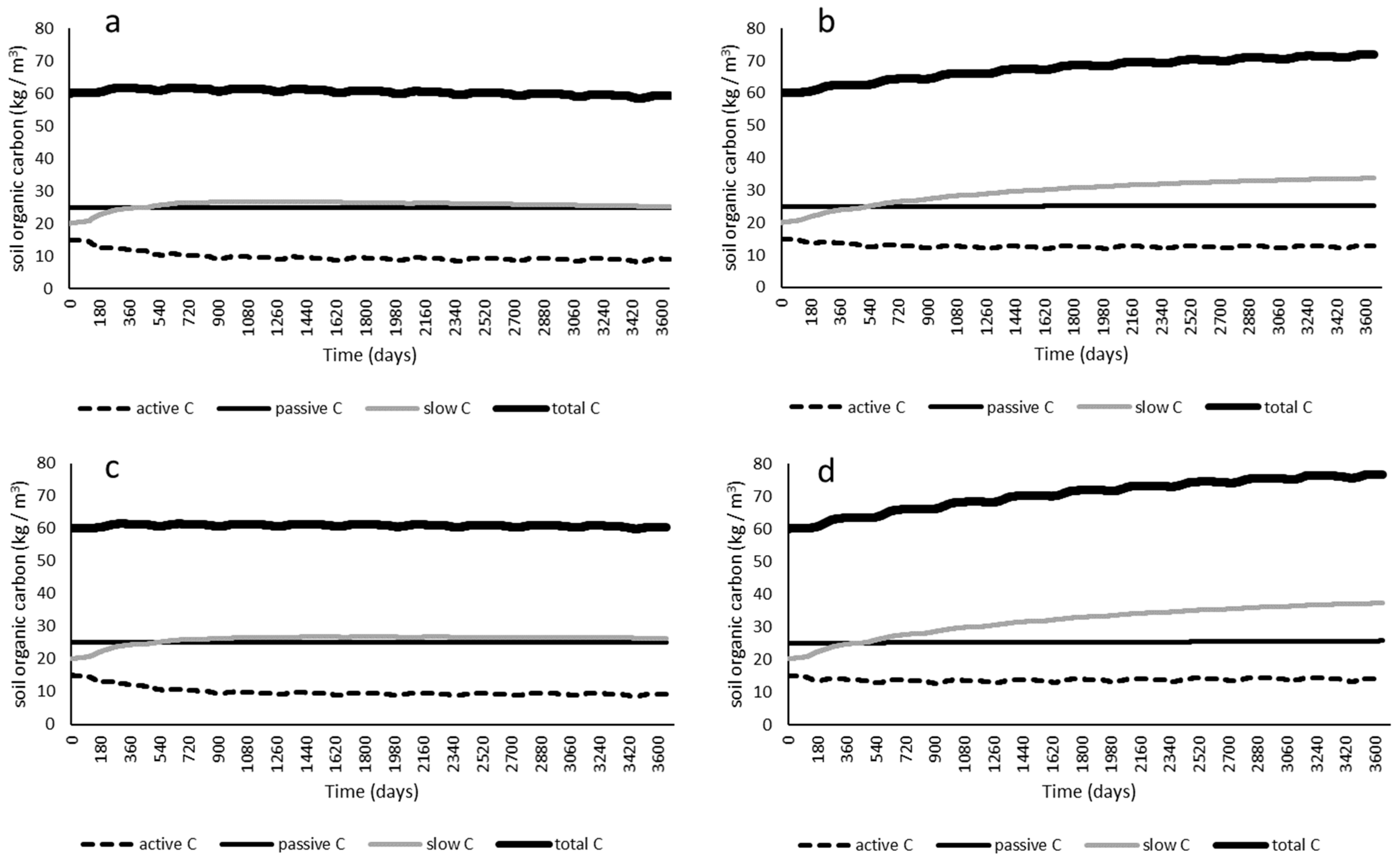
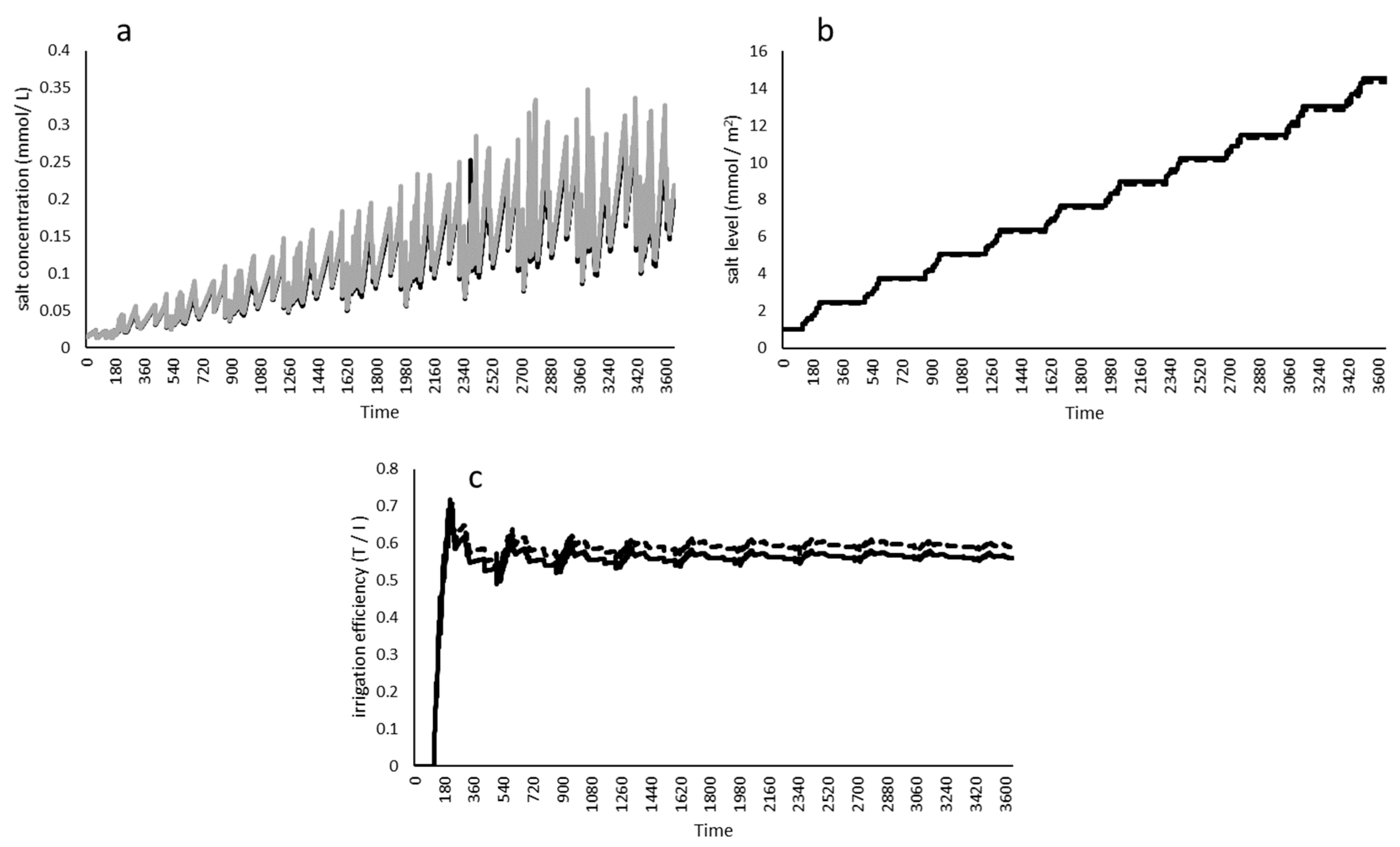
3.1. Why Do More Agricultural Producers Not Adopt Micro- or Drip Irrigation Systems?

Switching from the flood to drip irrigation method led to observable trade-offs between economic performance and soil system function driving the dynamics of nutrient cycling (Figure 7 and Figure 8).

Due to greater costs associated with drip irrigation equipment and labor to implement the drip irrigation system, profitability, although positive, was reduced relative to the flood method (Figure 7a). Because of this initial reduction in profit, the decision heuristic response led to relaxing the conditions needed to induce in-season irrigation application changes (Figure 7b) by reducing the soil moisture threshold needed to induce irrigation and increasing the target soil moisture level at which point irrigation ceases. Despite these conditions, cumulative irrigation with the drip system was less than half of the flood system (Figure 7c), while cumulative yield was slightly improved under drip irrigation (Figure 7d); the increased production rate did restore profitability beyond year two but not to the same level under the base case (Figure 7a). Mean soil moisture levels, irrigation efficiencies, and dissolved salt concentrations are given in Appendix A. Observable changes in soil nutrient stocks important to biogeochemical cycling seen after onset of drip irrigation. Soil nitrogen (N) reached a higher equilibrium after year one compared to the flood irrigation case (Figure 8a; spikes occur at fertilization events). Salt levels were significantly reduced due to reduced cumulative irrigation (Figure 8b). Under the flood irrigation system, flushing applications were required to offset via leaching the influence of salt accumulation, which also contributed to greater N leaching (Figure 8c). Soil organic matter (SOM), which was stable near 2.5% under flood irrigation, saw a linear increase to 3.5% under drip irrigation over the 10-year simulation experiment. These coupled dynamics show that reduced irrigation and flushing applications led to slightly greater N levels (due to reduction in leaching), contributing to marginal gains in crop productivity (Figure 7d). Greater crop biomass allowed more residue to be returned as surface and soil litter (which degraded less quickly due to the lower mean soil moisture), building SOM stock over time (Figure 8d). As SOM turned over, N availability increased with enhanced nitrification in the system, and more plant-available N reinforced crop productivity (Figure 8a).

Regarding the hypothesis that both agroecosystem function and economic outcomes will be improved under drip irrigation relative to flooding, we fail to reject the null hypothesis. Agroecosystem functions were improved (reduced leaching, greater N retention, greater SOM levels, lower irrigation-induced soil salinity). However, these functional improvements and small gains in crop productivity were not able to offset the additional cost of the drip irrigation system, resulting in less total profit compared to the base case.

3.2. Why Do More Agricultural Producers Not Adopt No-Tillage Practices in Their Crop Production Systems?

Switching from the conventional tillage practice to the no-tillage method produced significantly different economic and agronomic outcomes as well as those between soil system functions (Figure 9 and Figure 10). Profitability increased over time with the implementation of no-till (Figure 9a), a function of greater additional revenue generation from crop biomass harvest and sales (nonfruit, e.g., leaf and stem litter) not assumed in the conventional tillage case (Figure 9a), driven by the decision heuristic response to remove more biomass in response to changing profit in the first quarter of the experiment (Figure 9b). Cumulative yield was higher under no-till. However, the production rate was not increased after a four-year delay (Figure 9c), driven by a “reset” to the soil structure under no-till as observed in the mean soil pore radii (Figure 9d), which required approximately four years to reach a new stable state with a smaller pore radius as aggregation processes improved.

Changes in nutrient stocks important to biogeochemical cycling were also observed after implementation of no-tillage. Soil nitrogen levels began increasing after year three and reached a higher equilibrium compared to conventional tillage by year eight (Figure 10a). Salt levels remained unchanged (Figure 10b) while leaching was significantly reduced with no-till (Figure 10c). Soil organic matter (SOM), stable near 2.5% in the base case, grew linearly to over 3.5% under no-tillage (Figure 10d). No significant observable changes were seen in the soil moisture evolution (Figure 10e) or mean soil moisture (Figure 10f). These coupled dynamics show that reduced soil disturbance via no-tillage led to gradually greater N levels via the process of SOM accumulation and turnover, and that these improvements did lead to significant crop productivity gains after year three (Figure 9c). Greater crop biomass allowed more residue to be returned as surface and soil litter as well as for harvest, which contributed to significant shifts in profitability (Figure 9a). Soil salt levels and crop irrigation efficiency are given in Appendix A.

Regarding the hypothesis that both agroecosystem function and economic outcomes would be improved under no-tillage relative to conventional tillage, we fail to reject the null hypothesis. Profitability was improved in the experiment but not due to no-till. On the other hand, profit increased due to a managerial response to reduce litter turnover in favor of biomass harvest. The short-term delay between onset of no-till and improvement in agroecosystem functions (greater N retention and turnover, greater SOM levels) misled the economic decision-making elements in the model to value short-term economic results over longer-term outcomes beneficial to both financial and ecological components in the system. In addition, there was no observable improvement in soil moisture (a critical consideration in semi-arid environments which the model represents) despite improvements in other soil system processes.

3.3. Summary of the Nutrient Cycling Dynamics and Implications for Environmental Externalities

Interestingly, several similar dynamics in soil stocks or processes resulted from the drip irrigation or no-tillage test, albeit for different reasons and with unique implications regarding environmental externalities or their mitigation (Figure 11).

Under drip irrigation, soil moisture was significantly reduced and soil N and SOM enhanced (Figure 11). This bodes well for agroecosystems in arid and semi-arid regions facing increasing stress to water resources and demands to reduce agricultural water consumption in favor of conserving water for environmental flows (surface water systems), maximize net recharge (groundwater systems), and drought risk management for human use (both surface and groundwater systems). As indicated by the model results, these potential gains at the watershed-level must be weighed against trade-offs at the field level (given the feedback across scales). Although the cumulative salt level over time was reduced with drip irrigation, the in-growing-season dynamics were markedly similar (Figure 11 and Appendix A). This has implications for maintaining crop productivity in the long-term as even temporary salt accumulation (e.g., confined to the growing season) can negatively influence ET dynamics that drive crop production and yield, especially given the majority of irrigation water supplies are untreated.

No significant change in soil moisture dynamics was observed under no-tillage (Figure 11), and due to reduced leaching, led to marginally higher salt concentrations relative to conventional tillage (Figure 11). Reducing leaching, particularly of soil N, slows N flows into groundwater and streams that would mitigate water quality problems derived from N loading from agricultural systems, but like the drip irrigation case above, the trade-off may involve salt accumulation at field-scales. Importantly, no-tillage did improve soil N and SOM dynamics after a three-year delay (Figure 11) due to increased crop residue litter incorporation into soil C and N cycling (similar to [30,109] which showed one to five-year turnover time for plant residue pools). Because of this delay, many producers “lose patience”, prioritize immediate economic needs, and may abandon practices such as no-tillage with high crop residue litter in favor of conventional tillage or harvesting residues to generate new revenue potential (similar to the heuristic employed by the model). Agricultural influencers (extension, consultants, policy makers) will have to “fill this gap” of time from no-till implementation to the manifestation of productivity gains in innovative ways so that managers do not abandon practices before the cumulative benefits emerge.

Soil organic matter (SOM) dynamics were further partitioned into active C (one to five-year turnover times), slow C (20- to 40-year turnover times), and passive C states (200 to 1500-year turnover times) (similar to [93,94,95,110]). Both the irrigation and tillage base cases represented field conditions in relative equilibrium C conditions (Figure 12a,c) and in both treatments (drip irrigation or no-tillage), total soil C improved (Figure 12b,d): in the drip irrigation case, reduced soil moisture slowed soil respiration (a C outflow) while in the no-tillage case, greater plant residues led to greater provided greater soil litter (a C inflow), both of which allowed C accumulation into the slow C state.

4. Discussion

4.1. Viewing the Complexity of Soil Systems through an Integrative Lens

Soil systems, constituted by a unique matrix of physical, chemical and biological elements, organisms, and processes lie at the core foundation of agroecosystems that society relies on for the production of food and bioenergy as well as a much broader set of ecosystem goods and services that support all life. This paper provided an overview of soil systems through the lens of complex systems science and argued that soil is an archetype of complexity given observations about their known structure (physical, chemical, biological, and socio-economic) and behavior (arising from the interactions of these structural elements with managerial decision making; Figure 1). These characteristics included constantly changing, tightly coupled, governed by feedback, highly nonlinear, history dependent, self-organizing, adaptive, exhibiting trade-offs, and they express a high degree of counter-intuitiveness and resistance to policy or management changes. Particular attention was given to feedback processes and mechanisms across scales (from the rhizosphere to the watershed level). Due to the growing socio-economic pressures placed on agroecosystems globally as populations increase, the importance of soil and understanding the complex and dynamic structures that drive its ability to function (or those that contribute to its degradation) in conjunction with the decision-making influences of human managers are only going to become more critical if we are to mitigate soil-related externalities such as erosion, reduction in water holding capacity, loss of soil organic carbon, excessive fertilization and water runoff contamination, and soil salinization, among others. Additionally, hydroclimate variability further augments the already complex nature and behavior of soil systems.

We are therefore confronted with a dilemma: although we readily recognize the complexity of soil systems, it is well established from the systems sciences that the human mind is incapable of intuiting the full range of possible behaviors and trade-offs when confronted with such complexity. To cope with this, soil science as a discipline (like most others) has relied on reductionist approaches. Although productive in its knowledge generation of individual phenomena or descriptive characteristics, reliance on the reductionist approach has come with some unintended consequences, including the proliferation of “silos” that make integration of knowledge across different domains needed to understand the coupled, interactive dynamics of complex systems such as soils extremely difficult [10,13,21].

Given this challenge, we employ a systems approach, which by definition is holistic and integrative in nature and which facilitates communication across sub-disciplines within the field and with other disciplines. Utilizing the systems methodology argued for here has several advantages. First, the systems sciences have a well-developed working language useful for describing and communicating the underlying structure and dynamics of complex systems that is domain independent, allowing for translation and transfer of knowledge across disciplines. Examples from soil science and closely related fields include [48,49,51,52,57,91]. Translating existing knowledge about contemporary problem issues that cross cut soil and related disciplines, such as those problems outlined in Section 1.1.10 or in the case studies above, and how current scientists and managers are attempting to address such problems can be accelerated by harnessing this systems approach since its language and visual representation of feedback processes can: (a) facilitate discussion among stakeholders about perplexing issues and their underlying biological, chemical, and physical structures [111]; (b) capitalize on existing descriptions of problem structures that have been identified in other sciences, speeding up conceptualization and enhancing communication effectiveness of novel problems [112]; and (c) assist in creation of sustainable management strategies or crafting structural, causal scientific explanations to complicated observations through identification of compensating feedback processes—those that offset or regulate biogeochemical processes or defeat short-term management strategies [113].

Second, and building upon these conceptual elements, the systems approach provides a toolbox for operationalizing feedback processes into quantitative models useful for scientific investigations, especially where real-world experimentation is too costly, will take too long or require too much land or natural resources, or will be simply unethical. Constructing and employing such models is not a trivial process, but forces the investigator to: (a) make explicit formulations for underlying processes for all endogenous factors (i.e., everything within the model boundary), including socio-economic or decision-making elements contributing to the problem; (b) make explicit their unstated or unwritten assumptions, and those of the real-world stakeholders, undergirding the analysis; and (c) construct explicitly causal hypotheses about the behaviors of interest in the system and rigorously test them via simulation [91,92]. Augmenting these features of the systems process is the ability of most systems modeling platforms to interface with static models or databases in real time as well as the ability to create unique user-interfaces for education and extension efforts, which allow students or stakeholders direct access to the model and the ability to rapidly test new strategies or assumptions and see results of these changes instantaneously.

Finally, the systems approach specializes in properly accounting for the structures and effects of feedback. Reductionist approaches are most effective for systems that are summative, that is, “where the whole is equal to the sum of its parts”. In such systems, further reduction and analysis are the most efficient learning approach. On the other hand, complex systems that express the range of properties described above, including feedback, tend to produce interactive effects, also called emergent properties, that arise from the feedback network connecting different parts of a system, resulting in problems that are “more than the sum of their parts”.

Like any approach, there are drawbacks. Modeling complex systems often seems like a daunting task, especially for those individuals or teams not well versed in the language or methodologies. Disagreements may arise in determining the proper model boundary, the level of aggregation in model variables and feedbacks, the time horizon for analysis, among other important choices that must be made in any particular effort. For some variables, data needed to build confidence in resulting models may be inconsistent or lacking altogether. Developing understanding of the requisite sub-systems can take time, lengthening overall project lengths. Such weaknesses can be overcome with interdisciplinary teams working collaboratively (e.g., [8,9,48,49,53,54,75]), especially when at least one member is fluent in systems science who can serve to translate information between team members.

4.2. Case Study Modeling Applications: Insights, Strengths and Weaknesses

The presented model integrated across soil physical, chemical, and biological components and included economic factors relevant for agricultural production and decision making. The individual model components had been previously rigorously calibrated and evaluated for their performance against historical data. The novelty of the effort here was the integration of each model into a single, cohesive soil system model capturing feedbacks within and between soil physical, chemical, and biological processes and linking those with socio-economic outcomes and managerial decision-making feedbacks.

The model may be understood to be a “model system” or “proof of concept” from which general lessons may be drawn from wider ranging experimental conditions (including climates, soil types, and cropping systems) tested against current observations and future expectations. To help draw out some possible lessons, several case study simulations were run to evaluate the agroecosystem function and economic outcomes of drip irrigation (relative to flooding) and no-tillage cultivation (relative to conventional tillage) to better understand why agricultural producers may be reluctant to adopt such practices. These are critically important questions given recent agricultural producers surveys that have indicated that the adoption of no-tillage may be “flat-lining”, while cover cropping or multi-cropping has declined [67] and irrigation water use continues to increase [114].

Through these model experiments, we examined the soil system response and economic outcomes to varying input use (irrigation case) and management intensity (tillage case), with particular interest on the critical feedback processes between the soil system and management. Results from the tests showed fairly similar responses in soil N and SOM cycling albeit for markedly different reasons. In the irrigation case, N and SOM were enhanced due to reduced leaching and soil respiration. In the tillage case, N and SOM were enhanced due to greater crop litter turnover back into the soil system. The more interesting outcomes on the case study simulations centered on the economic impacts, which tended to be less favorable for managers. The reason for this lies in the recognition of compensating feedback between agroecosystem functions and economic decision making.

In the drip irrigation case, compensating feedback arose from the economic pressure felt by mangers due to increased investment costs, leading to greater irrigation applications. The assumed value of the irrigation investment ($250 per unit area relative to $5 per unit area under flooding) is also important. The difference in costs can be interpreted not only as a barrier to adoption for managers at the field level (Figure 3 and Figure 4) but also as a “shadow price” for what it would cost to mitigate environmental externalities from surface water or groundwater depletion and N and Na leaching or runoff at watershed scales (Figure 5). The more valuable insight, however, is how managers respond to the feedback of increased profit pressure—compensating with increased irrigation rates in attempt to maximize perceived productivity, which in water-stressed areas will only reinforce water conservation problems. Robust sensitivity analysis (which was beyond the scope of this paper) by varying the $250 irrigation investment assumption to specific costs of unique drip systems and geographic locations is something easily achieved through dynamic modeling frameworks as described here. When considering how the compensating feedback managers respond to it, it is more apparent why producers will remain averse to adopting the new technology.

In the tillage case, compensating feedback arose due to the opportunity costs of reduced harvest volumes to support nutrient cycling. Reduced harvest volumes enhanced N and SOM dynamics (Figure 9 and Figure 10), but maintaining the reduced fraction of biomass removal becomes economically challenging given the reduction in revenues compared to what could be attained with greater biomass sales. In response, management was led to market greater fractions of biomass over time than what was originally destined to be conserved as soil litter. As a result, profitability did rise relative to the base case, but this masks another important consideration. Given that in the conventional tillage control simulation, the ability to market biomass through multiple sales options was not included, the profit advantage illustrated in these results would evaporate had conventional tillage included both yield and crop residue revenues sources. When considering the compensating feedback managers respond to it should be much more apparent why producers will remain averse to no-till adoption or utilizing its benefits (e.g., enhanced nutrient cycling) to the largest extent possible.

In addition, neither the drip irrigation nor no-till case study simulations included the time and costs associated with learning how to use the new technology effectively or integrate it with existing management processes. For simplicity, these were not included in the analysis, but in reality, these must be considered as real costs (whether or not there is an explicit dollar value assigned), given managers must weigh the benefit–cost trade-offs when making their investment decisions.

Like any model, the one presented here possesses its own strengths and weaknesses. As already discussed, the high fidelity of soil processes and feedbacks between physical, chemical, biological, and socio-economics is a major strength. However, trade-offs in such high resolution of the soil feedbacks emerge. These include processes that are not well parameterized, such as feedbacks between soil aggregation and SOM dynamics or changes in soil horizonation (weaknesses that are shared among a host of soil models [115]), as well as those excluded from the model, such as plant rooting types and dynamics and basement controls on soil formation, which occur at much longer time-scales than shown here using a management-centric time horizon.

4.3. Frontiers in Soil Science Complexity Research and Education

An important lesson learnt from applying a systems approach to soils in this way is that it is only through evaluating non-reductionist hypotheses such as these (i.e., that include both agroecosystem and economic considerations and the feedbacks and they entail), that the investigator is forced to consider the full range of outcomes, interactions, and trade-offs before reaching conclusions. Objectively evaluating socio-economic and environmental trade-offs in soil system function with soil system outcomes illuminates the “white spaces” between scientific “silos”: where a soil scientist is led to conclude that conservation practices should be the norm because of the overall benefits to soil function and health, the soil economist is just as likely to be led to conclude that some conservation practices may not pay for themselves economically and therefore those practices should be used more selectively. It is this “breaking out of silos” that many others have emphasized at philosophical or conceptual levels [10,13,21]; this paper illustrated how a systems approach can operationalize it.

The modern challenge for agricultural, soil, and natural resource management, that is, to feed a growing global population with less land, water, energy, inputs, and environmental impact, has spurred renewed interest in and emphasis on soil systems from both scientific communities and the general public alike. The emerging soil health and soil security movements have brought to light a number of new frontiers on the horizon that can be explored by leveraging a systems approach to help meet the challenge. These include evaluations of investments in soil health and the resulting impact to soil functional processes and environmental outcomes. Much of this work is currently being performed in traditional experimental conditions, e.g., field-level applications such as variable rate fertilization, deficit irrigation strategies, fertigation, integrating cover crops and livestock in conventional agricultural systems, or larger-scale monitoring of problems such as nutrient loading in watersheds or climate change mitigation potential from alternative management strategies. As was shown here, the systems modeling frameworks have an important role to play given: (a) the time, cost, and logistical challenges often encountered in traditional approaches mentioned above; and (b) the systems sciences have a well-established working language and have crystallized particular observations about complex systems that will aid in conceptualizing, quantifying, and communicating to others about soil system dynamics, its links to ecosystem goods and services, including biogeochemical cycling, and evaluating management trade-offs needed to mitigate externalities. Finally, the dynamic decision-making characteristics of decision makers (producers and policy makers) that lead to investments in sustainable soil system management practices conducive to enhancing achievement of desired outcomes at plot, field, and watershed scales (and the feedbacks between them, Figure 2, Figure 3, Figure 4 and Figure 5) need to be better understood and captured in soil system research of all kinds. Modeling these complex, coupled natural–human system problems, in agroecosystems or elsewhere, remains an important transdisciplinary endeavor that all soil scientists will have an integral part to play in.

5. Conclusions

Effective soil management requires the knowledge and ability to examine and understand, evaluate, and then manage the complex, dynamic (often nonlinear) trade-offs that characterize soil systems. There were two primary aims of this paper. First, we set out to describe a theoretical foundation, translated from the complexity sciences, from which inter- and transdisciplinary soil science work can build upon to more effectively investigate, understand, and manage soil system characteristics (Section 1, particularly Section 1.1.1, Section 1.1.2, Section 1.1.3, Section 1.1.4, Section 1.1.5, Section 1.1.6, Section 1.1.7, Section 1.1.8, Section 1.1.9 and Section 1.1.10), especially the principle that systems are governed by feedback, and to provide a language by which complex soil features can be communicated across disciplines. Second, we illustrated how a holistic modeling effort can effectively operationalize this systems perspective via integration of dynamic soil feedback processes (Section 2 and Section 3). The mathematical model demonstrated the complex, feedback-driven relationships central to many soil system processes and was used to illustrate two case studies harnessing the power of the model to explore pressing contemporary agroecosystem problems relevant to biogeochemical cycling and environmental externalities. Modeling agroecosystems in this way remains an area needed in development if we are to improve our understanding of and ability to manage complex resource management problems including, but not limited to, irrigation, fertilization, soil salinity, soil erosion and/or compaction that continue to plague agroecosystems around the world. The contribution and impact of such models will be augmented with the integration of biogeochemical components with socio-economic and decision-making factors relevant to the issue at hand.

References

1. Matson, P.A. Agricultural Intensification and Ecosystem Properties. Science. 1997, 277, 504–509. [Google Scholar] [CrossRef] [PubMed] [Green Version]
2. Hartemink, A.E.; McBratney, A. A soil science renaissance. Geoderma 2008, 148, 123–129. [Google Scholar] [CrossRef]
3. Schröder, J.J.; Schulte, R.P.; Creamer, R.E.; Delgado, A.; Leeuwen, J.; Lehtinen, T. The elusive role of soil quality in nutrient cycling: A review. Soil Use Manag. 2016, 32, 476–486. [Google Scholar] [CrossRef]
4. Adhikari, K.; Hartemink, A.E. Linking soils to ecosystem services—A global review. Geoderma 2016, 262, 101–111. [Google Scholar] [CrossRef]
5. Power, A.G. Ecosystem services and agriculture: Tradeoffs and synergies. Philos. Trans. R. Soc. B 2010, 365, 2959–2971. [Google Scholar] [CrossRef]
6. Swift, M.J.; Izac, A.-M.N.; van Noordwijk, M. Biodiversity and ecosystem services in agricultural landscapes—are we asking the right questions? Agric. Ecosyst. Environ. 2004, 104, 113–134. [Google Scholar] [CrossRef]
7. Alexander, P.; Rounsevell, M.D.; Dislich, C.; Dodson, J.R.; Engström, K.; Moran, D. Drivers for global agricultural land use change: The nexus of diet; population; yield and bioenergy. Glob. Environ. Chang. 2015, 35, 138–147. [Google Scholar] [CrossRef] [Green Version]
8. Turner, B.L.; Fuhrer, J.; Wuellner, M.; Menendez, H.M.; Dunn, B.H.; Gates, R. Scientific case studies in land-use driven soil erosion in the central United States: Why soil potential and risk concepts should be included in the principles of soil health. Int. Soil Water Conserv. Res. 2018, 6, 63–78. [Google Scholar] [CrossRef]
9. Turner, B.L.; Wuellner, M.; Malo, D.D.; Herrick, J.E.; Dunn, B.H.; Gates, R. Ecosystem functions in mixed cropland–grassland systems influenced by soil legacies of past crop cultivation decisions. Ecosphere. 2018, 9, e02521. [Google Scholar] [CrossRef]
10. Vogel, H.-J.; Bartke, S.; Daedlow, K.; Helming, K.; Kögel-Knabner, I.; Lang, B. A systemic approach for modeling soil functions. SOIL 2018, 4, 83–92. [Google Scholar] [CrossRef] [Green Version]
11. Adewopo, J.B.; VanZomeren, C.; Bhomia, R.K.; Almaraz, M.; Bacon, A.R.; Eggleston, E. Top-Ranked Priority Research Questions for Soil Science in the 21st Century. Soil Sci. Soc. Am. J. 2014, 78, 337–347. [Google Scholar] [CrossRef] [Green Version]
12. Baveye, P.C. Grand challenges in the research on soil processes. Front. Environ. Sci. 2015, 3. [Google Scholar] [CrossRef] [Green Version]
13. Bridges, E.M.; Catizzone, M. Soil science in a holistic framework: Discussion of an improved integrated approach. Geoderma 1996, 71, 275–287. [Google Scholar] [CrossRef]
14. Sterman, J.D. System Dynamics Modeling: Tools for Learning in a Complex World. Calif. Manag. Rev. 2001, 43, 8–25. [Google Scholar] [CrossRef]
15. Sterman, J.D. Sustaining Sustainability: Creating a Systems Science in a Fragmented Academy and Polarized World. In Sustainability Science; Springer: New York, NY, USA, 2012; pp. 21–58. [Google Scholar] [CrossRef]
16. Foster, J. From simplistic to complex systems in economics. Camb. J. Econ. 2005, 29, 873–892. [Google Scholar] [CrossRef] [Green Version]
17. Turner, B.L.; Goodman, M.; Machen, R.; Mathis, C.; Rhoades, R.; Dunn, B. Results of Beer Game Trials Played by Natural Resource Managers Versus Students: Does Age Influence Ordering Decisions? Systems 2020, 8, 37. [Google Scholar] [CrossRef]
18. Kahneman, D. Thinking Fast and Slow; Farrar, Straus and Giroux: New York, NY, USA, 2011. [Google Scholar]
19. Cronin, M.A.; Gonzalez, C.; Sterman, J.D. Why don’t well-educated adults understand accumulation? A challenge to researchers, educators, and citizens. Organ. Behav. Hum. Decis. Process. 2009, 108, 116–130. [Google Scholar] [CrossRef]
20. Manzoni, S.; Porporato, A.; D’Odorico, P.; Laio, F.; Rodriguez-Iturbe, I. Soil nutrient cycles as a nonlinear dynamical system. Nonlinear Process. Geophys. 2004, 11, 589–598. [Google Scholar] [CrossRef] [Green Version]
21. Churchman, G.J. The philosophical status of soil science. Geoderma 2010, 157, 214–221. [Google Scholar] [CrossRef]
22. Senge, P.M. The leader’s new work: Building learning organizations. Sloan Manag. Rev. 1990, 31, 7–23. [Google Scholar]
23. Barlas, Y. System dynamics: Systemic feedback modeling for policy analysis. System 2007, 1, 1–29. [Google Scholar]
24. Sterman, J.D. Learning in and about complex systems. Syst. Dyn. Rev. 1994, 10, 291–330. [Google Scholar] [CrossRef] [Green Version]
25. Bar-Yam, Y. General features of complex systems. In Encyclopeida of Life Support Systems (EOLSS); UNESCO, EOLSS Pubblishers: Oxford, UK, 2002. [Google Scholar]
26. Stockmann, U.; Minasny, B.; McBratney, A.B. How fast does soil grow? Geoderma 2014, 216, 48–61. [Google Scholar] [CrossRef]
27. Montgomery, D.R. Soil erosion and agricultural sustainability. Proc. Natl. Acad. Sci. USA 2007, 104, 13268–13272. [Google Scholar] [CrossRef] [Green Version]
28. Montgomery, D.R. Dirt: The Erosion of Civilizations; University of California Press: Oakland, CA, USA, 2007. [Google Scholar]
29. Zhang, R.; Wienhold, B.J. The effect of soil moisture on mineral nitrogen, soil electrical conductivity, and pH. Nutr. Cycl. Agroecosyst. 2002, 63, 251–254. [Google Scholar] [CrossRef]
30. Zhang, K.; Maltais-Landry, G.; Liao, H.-L. How soil biota regulate C cycling and soil C pools in diversified crop rotations. Soil Biol. Biochem. 2021, 156, 108219. [Google Scholar] [CrossRef]
31. Balestrini, R.; Lumini, E.; Borriello, R.; Bianciotto, V. Plant-Soil Biota Interactions. In Soil Microbiology; Ecology and Biochemistry; Elsevier: Amsterdam, The Netherlands, 2015; pp. 311–338. [Google Scholar] [CrossRef]
32. Wagg, C.; Bender, S.F.; Widmer, F.; van der Heijden, M.G. Soil biodiversity and soil community composition determine ecosystem multifunctionality. Proc. Natl. Acad. Sci. USA 2014, 111, 5266–5270. [Google Scholar] [CrossRef] [PubMed] [Green Version]
33. Bücking, H.; Kafle, A. Role of Arbuscular Mycorrhizal Fungi in the Nitrogen Uptake of Plants: Current Knowledge and Research Gaps. Agronomy 2015, 5, 587–612. [Google Scholar] [CrossRef] [Green Version]
34. Massalha, H.; Korenblum, E.; Tholl, D.; Aharoni, A. Small molecules below-ground: The role of specialized metabolites in the rhizosphere. Plant J. 2017, 90, 788–807. [Google Scholar] [CrossRef] [Green Version]
35. Giovannini, L.; Palla, M.; Agnolucci, M.; Avio, L.; Sbrana, C.; Turrini, A. Arbuscular Mycorrhizal Fungi and Associated Microbiota as Plant Biostimulants: Research Strategies for the Selection of the Best Performing Inocula. Agronomy 2020, 10, 106. [Google Scholar] [CrossRef] [Green Version]
36. Chandra, P. Soil-Microbes-Plants: Interactions and ecological diversity. In Plant Microbes Interface; Springer: Cham, Switzerland; pp. 145–176.
37. Turner, B.L.; Kodali, S. Soil system dynamics for learning about complex; feedback-driven agricultural resource problems: Model development, evaluation, and sensitivity analysis of biophysical feedbacks. Ecol. Model. 2020, 428, 109050. [Google Scholar] [CrossRef]
38. Laio, F.; Porporato, A.; Ridolfi, L.; Rodriguez-Iturbe, I. Plants in water-controlled ecosystems: Active role in hydrologic processes and response to water stress II. Probabilistic soil moisture dynamics. Adv. Water Resour. 2001, 24, 707–723. [Google Scholar] [CrossRef]
39. Porporato, A.; Laio, F.; Ridolfi, L.; Rodriguez-Iturbe, I. Plants in water-controlled ecosystems: Active role in hydrologic processes and response to water stress III. Vegetation water stress. Adv. Water Resour. 2001, 24, 725–744. [Google Scholar] [CrossRef]
40. Laio, F.; Porporato, A.; Fernandez-Illescas, C.P.; Rodriguez-Iturbe, I. Plants in water-controlled ecosystems: Active role in hydrologic processes and response to water stress IV. Discussion of real cases. Adv. Water Resour. 2001, 24, 745–762. [Google Scholar] [CrossRef]
41. Rodríguez-Iturbe, I.; Porporato, A. Ecohydrology of Water-Controlled Ecosystems; Cambridge University Press: Cambridge, UK, 2005. [Google Scholar] [CrossRef]
42. Manzoni, S.; Porporato, A. Soil carbon and nitrogen mineralization: Theory and models across scales. Soil Biol. Biochem. 2009, 41, 1355–1379. [Google Scholar] [CrossRef]
43. Mau, Y.; Porporato, A. A dynamical system approach to soil salinity and sodicity. Adv. Water Resour. 2015, 83, 68–76. [Google Scholar] [CrossRef] [Green Version]
44. Pelak, N.; Revelli, R.; Porporato, A. A dynamical systems framework for crop models: Toward optimal fertilization and irrigation strategies under climatic variability. Ecol. Model. 2017, 365, 80–92. [Google Scholar] [CrossRef] [Green Version]
45. Pelak, N.; Porporato, A. Dynamic evolution of the soil pore size distribution and its connection to soil management and biogeochemical processes. Adv. Water Resour. 2019, 131, 103384. [Google Scholar] [CrossRef]
46. Porporato, A.; Feng, X.; Manzoni, S.; Mau, Y.; Parolari, A.J.; Vico, G. Ecohydrological modeling in agroecosystems: Examples and challenges. Water Resour. Res. 2015, 51, 5081–5099. [Google Scholar] [CrossRef] [Green Version]
47. Forrester, J.W. Policies, decisions and information sources for modeling. Eur. J. Oper. Res. 1992, 59, 42–63. [Google Scholar] [CrossRef]
48. Fernald, A.; Tidwell, V.; Rivera, J.; Rodríguez, S.; Guldan, S.; Steele, C.; Ochoa, C.; Hurd, B.; Ortiz, M.; Boykin, K.; et al. Modeling Sustainability of Water, Environment, Livelihood, and Culture in Traditional Irrigation Communities and Their Linked Watersheds. Sustainability 2012, 4, 2998–3022. [Google Scholar] [CrossRef] [Green Version]
49. Gunda, T.; Turner, B.L.; Tidwell, V.C. The Influential Role of Sociocultural Feedbacks on Community-Managed Irrigation System Behaviors During Times of Water Stress. Water Resour. Res. 2018, 54, 2697–2714. [Google Scholar] [CrossRef]
50. Ferguson, I.M.; Maxwell, R.M. Role of groundwater in watershed response and land surface feedbacks under climate change. Water Resour. Res. 2010, 46. [Google Scholar] [CrossRef]
51. Hooper, B.P.; Lant, C. Integrated, Adaptive Watershed Management. In Fostering Integration: Concepts and Practice in Resource and Environmental Management; Hanna, K., Scott Slocombe, D., Eds.; Oxford University Press: Oxford, UK; Toronto, ON, Canada, 2007. [Google Scholar]
52. Calkin, D.E.; Thompson, M.P.; Finney, M.A. Negative consequences of positive feedbacks in US wildfire management. For Ecosyst. 2015, 2, 1–10. [Google Scholar] [CrossRef] [Green Version]
53. Fernald, A.G.; Cevik, S.Y.; Ochoa, C.G.; Tidwell, V.C.; King, J.P.; Guldan, S.J. River Hydrograph Retransmission Functions of Irrigated Valley Surface Water–Groundwater Interactions. J. Irrig. Drain. Eng. 2010, 136, 823–835. [Google Scholar] [CrossRef]
54. Fernald, A.; Guldan, S.; Boykin, K.; Cibils, A.; Gonzales, M.; Hurd, B.; Lopez, S.; Ochoa, C.; Ortiz, M.; Rivera, J.; et al. Linked hydrologic and social systems that support resilience of traditional irrigation communities. Hydrol. Earth Syst. Sci. 2015, 19, 293–307. [Google Scholar] [CrossRef] [Green Version]
55. Ochoa, C.G.; Guldan, S.J.; Cibils, A.F.; Lopez, S.C.; Boykin, K.G.; Tidwell, V.C.; Fernald, A.G. Hydrologic Connectivity of Head Waters and Floodplains in a Semi-Arid Watershed. J. Contemp. Water Res. Educ. 2013, 152, 69–78. [Google Scholar] [CrossRef]
56. Menendez, H.M.; Wuellner, M.R.; Turner, B.L.; Gates, R.N.; Dunn, B.H.; Tedeschi, L.O. A spatial landscape scale approach for estimated erosion, water quantity, and quality in response to South Dakota grassland conversion. Nat. Resour. Model. 2019, 33, e12243. [Google Scholar] [CrossRef]
57. Popp, A.; Blaum, N.; Jeltsch, F. Ecohydrological feedback mechanisms in arid rangelands: Simulating the impacts of topography and land use. Basic Appl. Ecol. 2009, 10, 319–329. [Google Scholar] [CrossRef]
58. Yang, Y.; Lin, J.; Liu, G.; Zhou, L. The behavioural causes of bullwhip effect in supply chains: A systematic literature review. Int. J. Prod. Econ. 2021, 236, 108120. [Google Scholar] [CrossRef]
59. Jenny, H. Factors of Soil Formation: A System of Quantitative Pedology; Dover Publications, Inc.: New York, NY, USA, 1994. [Google Scholar]
60. Kaisermann, A.; Vries, F.T.; Griffiths, R.I.; Bardgett, R.D. Legacy effects of drought on plant–soil feedbacks and plant–plant interactions. New Phytol. 2017, 215, 1413–1424. [Google Scholar] [CrossRef] [Green Version]
61. Kleinschroth, F.; Gourlet-Fleury, S.; Sist, P.; Mortier, F.; Healey, J.R. Legacy of logging roads in the Congo Basin: How persistent are the scars in forest cover? Ecosphere 2015, 6, 1–17. [Google Scholar] [CrossRef] [Green Version]
62. Monger, C.; Sala, O.E.; Duniway, M.C.; Goldfus, H.; Meir, I.A.; Poch, R.M.; Throop, H.L.; Vivoni, E.R. Legacy effects in linked ecological–soil–geomorphic systems of drylands. Front. Ecol. Environ. 2015, 13, 13–19. [Google Scholar] [CrossRef] [Green Version]
63. Steel, Z.L.; Safford, H.D.; Viers, J.H. The fire frequency-severity relationship and the legacy of fire suppression in California forests. Ecosphere 2015, 6, 1–23. [Google Scholar] [CrossRef]
64. Angeler, D.G.; Fried-Petersen, H.B.; Allen, C.R.; Garmestani, A.; Twidwell, D.; Chuang, W.-C.; Donovan, V.M.; Eason, T.; Roberts, C.P.; Sundstrom, S.M.; et al. Adaptive capacity in ecosystems. In Resilience in Complex Socio-Ecological Systems; Elsevier: Amsterdam, The Netherlands, 2019; pp. 1–24. [Google Scholar] [CrossRef]
65. Holling, C.S. Simplifying the complex: The paradigms of ecological function and structure. Eur. J. Oper. Res. 1987, 30, 139–146. [Google Scholar] [CrossRef]
66. Zhang, D.; Peng, Y.; Li, F.; Yang, G.; Wang, J.; Yu, J.; Zhou, G.; Yang, Y. Changes in above-/below-ground biodiversity and plant functional composition mediate soil respiration response to nitrogen input. Funct. Ecol. 2021, 35, 1171–1182. [Google Scholar] [CrossRef]
67. Wade, T.; Classen, R.; Wallander, S. Conservation-Practice Adoption Rates Vary Widely by Crop and Region; EIB-147; U.S. Department of Agriculture, Economic Research Service: Washington, DC, USA, 2015.
68. Ward, P.S.; Bell, A.R.; Droppelmann, K.; Benton, T.G. Early adoption of conservation agriculture practices: Understanding partial compliance in programs with multiple adoption decisions. Land Use Policy 2018, 70, 27–37. [Google Scholar] [CrossRef]
69. Lahmar, R. Adoption of conservation agriculture in Europe. Land Use Policy 2010, 27, 4–10. [Google Scholar] [CrossRef]
70. Knowler, D.; Bradshaw, B. Farmers’ adoption of conservation agriculture: A review and synthesis of recent research. Food Policy 2007, 32, 25–48. [Google Scholar] [CrossRef]
71. Giller, K.E.; Andersson, J.A.; Corbeels, M.; Kirkegaard, J.; Mortensen, D.; Erenstein, O.; Vanlauwe, B. Beyond conservation agriculture. Front. Plant Sci. 2015, 6, 870. [Google Scholar] [CrossRef] [Green Version]
72. Pittelkow, C.M.; Linquist, B.A.; Lundy, M.E.; Liang, X.; van Groenigen, K.J.; Lee, J.; van Gestal, N.; Six, J.; Venterea, R.T.; van Kessel, C. When does no-till yield more? A global meta-analysis. Field Crop. Res. 2015, 183, 156–168. [Google Scholar] [CrossRef] [Green Version]
73. Ismail, I.; Blevins, R.L.; Frye, W.W. Long-Term No-tillage Effects on Soil Properties and Continuous Corn Yields. Soil Sci. Soc. Am. J. 1994, 58, 193–198. [Google Scholar] [CrossRef]
74. West, T.O.; Post, W.M. Soil Organic Carbon Sequestration Rates by Tillage and Crop Rotation. Soil Sci. Soc. Am. J. 2002, 66, 1930–1946. [Google Scholar] [CrossRef] [Green Version]
75. Turner, B.L.; Wuellner, M.; Nichols, T.; Gates, R. Dueling Land Ethics: Uncovering Agricultural Stakeholder Mental Models to Better Understand Recent Land Use Conversion. J. Agric. Environ. Ethics 2014, 27, 831–856. [Google Scholar] [CrossRef]
76. Wright, C.K.; Wimberly, M.C. Recent land use change in the Western Corn Belt threatens grasslands and wetlands. Proc. Natl. Acad. Sci. USA 2013, 110, 4134–4139. [Google Scholar] [CrossRef] [Green Version]
77. Gilovich, T.; Griffin, D.; Kahneman, D. (Eds.) Heuristics and Biases: The Psychology of Intuitive Judgment; Cambridge University Press: Cambridge, UK, 2002. [Google Scholar]
78. Tversky, A.; Kahneman, D. Judgment under Uncertainty: Heuristics and Biases. Science 1974, 185, 1124–1131. [Google Scholar] [CrossRef]
79. Malik, Z.; Ahmad, M.; Abassi, G.H.; Dawood, M.; Hussain, A.; Jamil, M. Agrochemicals and Soil Microbes: Interaction for Soil Health. In Soil Biology; Springer International Publishing: New York, NY, USA, 2017; pp. 139–152. [Google Scholar] [CrossRef]
80. Wood, S.A.; Bradford, M.A.; Gilbert, J.A.; McGuire, K.L.; Palm, C.A.; Tully, K.L.; Zhou, J.; Naeem, S. Agricultural intensification and the functional capacity of soil microbes on smallholder African farms. J. Appl. Ecol. 2015, 52, 744–752. [Google Scholar] [CrossRef]
81. Hartmann, M.; Frey, B.; Mayer, J.; Mäder, P.; Widmer, F. Distinct soil microbial diversity under long-term organic and conventional farming. ISME J. 2014, 9, 1177–1194. [Google Scholar] [CrossRef] [PubMed] [Green Version]
82. Maas, E.V. Salt tolerance of plants. In Handbook of Plant Science in Agriculture; Christie, B.R., Ed.; CRC Press: Boca Raton, FL, USA, 1987; Volume 2, pp. 57–75. [Google Scholar]
83. Abrol, I.P.; Yadav, J.S.; Massoud, F.I. Salt-Affected Soils and Their Management; FAO Soils Bulletin 39; Food & Agriculture Organization: Rome, Italy, 1988. [Google Scholar]
84. Bernstein, L. Effects of Salinity and Sodicity on Plant Growth. Annu. Rev. Phytopathol. 1975, 13, 295–312. [Google Scholar] [CrossRef]
85. Levy, G.J. Sodicity. In Handbook of Soil Sciences: Resource Management and Environmental Impacts; Huang, P.M., Li, Y., Sumner, M.E., Eds.; CRC Press: Boca Raton, FL, USA, 2012. [Google Scholar] [CrossRef]
86. Ghassemi, F.; Jakeman, A.J.; Nix, H.A. Salinisation of Land and Water Resources: Human Causes, Extent, Management and Case Studies; Cab International: Wallingford, UK, 1995. [Google Scholar]
87. Bekle, H.; Mulcock, J.; Phillips, H. The Salinity Crisis: Landscapes, Communities and Politics; UWA Publishing: Crawley, Australia, 2004. [Google Scholar]
88. Abbas, F.; Hammad, H.M.; Ishaq, W.; Farooque, A.A.; Bakhat, H.F.; Zia, Z.; Fahad, S.; Farhad, W.; Cerdà, A. A review of soil carbon dynamics resulting from agricultural practices. J. Environ. Manag. 2020, 268, 110319. [Google Scholar] [CrossRef] [PubMed]
89. Lowdermilk, W.C. Conquest of the Land through 7000 Years: (No. 99); Soil Conservation Service, US Department of Agriculture: Washington, DC, USA, 1953.
90. Kookana, R.S.; Sarmah, A.K.; Van Zwieten, L.; Krull, E.; Singh, B. Biochar Application to Soil. In Advances in Agronomy; Elsevier: Amsterdam, The Netherlands, 2011; pp. 103–143. [Google Scholar] [CrossRef]
91. Turner, B.; Menendez, H.; Gates, R.; Tedeschi, L.; Atzori, A. System Dynamics Modeling for Agricultural and Natural Resource Management Issues: Review of Some Past Cases and Forecasting Future Roles. Resources 2016, 5, 40. [Google Scholar] [CrossRef] [Green Version]
92. Turner, B.L. Model laboratories: A quick-start guide for design of simulation experiments for dynamic systems models. Ecol. Model. 2020, 434, 109246. [Google Scholar] [CrossRef]
93. Parton, W.J.; Schimel, D.S.; Cole, C.V.; Ojima, D.S. Analysis of factors controlling soil organic matter levels in Great Plains grasslands. Soil Sci. Soc. Am. J. 1987, 51, 1173–1179. [Google Scholar] [CrossRef]
94. Parton, W.J.; Ojima, D.S.; Cole, C.V.; Schimel, D.S. A General Model for Soil Organic Matter Dynamics: Sensitivity to Litter Chemistry, Texture and Management. In Quantitative Modeling of Soil Forming Processes; Soil Science Society of America: Madison, WI, USA, 1994; pp. 147–167. [Google Scholar] [CrossRef] [Green Version]
95. Parton, W.J. The CENTURY model. In Evaluation of Soil Organic Matter Models; Springer: Berlin/Heidelberg, Germany, 1996; pp. 283–291. [Google Scholar] [CrossRef]
96. Clapp, R.B.; Hornberger, G.M. Empirical equations for some soil hydraulic properties. Water Resour. Res. 1978, 14, 601–604. [Google Scholar] [CrossRef] [Green Version]
97. Mualem, Y.; Dagan, G. Hydraulic Conductivity of Soils: Unified Approach to the Statistical Models. Soil Sci. Soc. Am. J. 1978, 42, 392–395. [Google Scholar] [CrossRef]
98. Mohaghegh, M.; Größler, A. The Dynamics of Operational Problem-Solving: A Dual-Process Approach. Syst. Pract. Action Res. 2019, 33, 27–54. [Google Scholar] [CrossRef]
99. Choo, A.S. Defining Problems Fast and Slow: The U-shaped Effect of Problem Definition Time on Project Duration. Prod. Oper. Manag. 2014, 23, 1462–1479. [Google Scholar] [CrossRef]
100. Repenning, N.P.; Sterman, J.D. Capability Traps and Self-Confirming Attribution Errors in the Dynamics of Process Improvement. Adm. Sci. Q. 2002, 47, 265. [Google Scholar] [CrossRef]
101. Althoff, T.D.; Menezes, R.S.; de Pinto, A.S.; Pareyn, F.G.; de Carvalho, A.L.; Martins, J.C.; Carvalho, E.; Samuel, A.; da Silva, A.; Dutra, E.; et al. Adaptation of the century model to simulate C and N dynamics of Caatinga dry forest before and after deforestation. Agric. Ecosyst. Environ. 2018, 254, 26–34. [Google Scholar] [CrossRef]
102. Dimassi, B.; Guenet, B.; Saby, N.P.; Munoz, F.; Bardy, M.; Millet, F.; Martin, M.P. The impacts of CENTURY model initialization scenarios on soil organic carbon dynamics simulation in French long-term experiments. Geoderma 2018, 311, 25–36. [Google Scholar] [CrossRef]
103. Nicoloso, R.S.; Amado, T.J.; Rice, C.W. Assessing strategies to enhance soil carbon sequestration with the DSSAT-CENTURY model. Eur. J. Soil Sci. 2020, 71, 1034–1049. [Google Scholar] [CrossRef]
104. Franzluebbers, A.J.; Follett, R.F.; Johnson, J.M.; Liebig, M.A.; Gregorich, E.G.; Parkin, T.B.; Smith, J.L.; Del Grosso, S.J.; Jawson, M.D.; Martens, D.A. Agricultural exhaust: A reason to invest in soil. J. Soil Water Conserv. 2006, 61, 98A–101A. [Google Scholar]
105. Six, J.; Conant, R.T.; Paul, E.A.; Paustian, K. Stabilization mechanisms of soil organic matter: Implications for C-saturation of soils. Plant Soil 2002, 241, 155–176. [Google Scholar] [CrossRef]
106. Delgado, J.A. Crop residue is a key for sustaining maximum food production and for conservation of our biosphere. J. Soil Water Conserv. 2010, 65, 111A–116A. [Google Scholar] [CrossRef] [Green Version]
107. Smith, P.; House, J.I.; Bustamante, M.; Sobocká, J.; Harper, R.; Pan, G.; West, P.C.; Clark, J.M.; Adhya, T.; Rumpel, C.; et al. Global change pressures on soils from land use and management. Glob. Chang. Biol. 2015, 22, 1008–1028. [Google Scholar] [CrossRef]
108. Franzluebbers, A.J.; Wendroth, O.; Creamer, N.G.; Feng, G.G. Focusing the future of farming on agroecology. Agric. Environ. Lett. 2020, 5, e20034. [Google Scholar] [CrossRef]
109. McGill, W.B.; Hunt, W.W.; Woodmansee, R.G.; Reuss, J.O. PHOENIX, a model of the dynamics of carbon and nitrogen in grassland soils. Ecol. Bull. 1981, 33, 49–115. [Google Scholar]
110. Martin, J.P.; Haider, K. Influence of mineral colloids on turnover rates of soil organic carbon. In Interactions of Soil Minerals with Natural Organics and Microbes; Huang, P.M., Schnitzer, M., Eds.; Soil Science Society of America Special Publication 17; SSSA: Madison, WI, USA, 1986; pp. 283–304. [Google Scholar]
111. Lane, D. Can we have confidence in generic structure? J. Oper. Res. Soc. 1998, 49, 936–947. [Google Scholar] [CrossRef]
112. Senge, P. The Fifth Discipline, The Art and Practice of the Learning Organization; Currency/Doubleday: New York, NY, USA, 1990. [Google Scholar]
113. Richardson, G.P. System Dynamics. In Encyclopedia of Operations Research and Management Science; Springer Science and Business Media: Berlin, Germany, 2013; pp. 1519–1522. [Google Scholar] [CrossRef]
114. United States Department of Agriculture. Farm and Ranch Irrigation Survey 2013. Special Studies, Part 1, AC-12-SS-1; November 2014; Volume 3. Available online: https://www.nass.usda.gov/Publications/AgCensus/2012/Online_Resources/Farm_and_Ranch_Irrigation_Survey/ (accessed on 20 October 2019).
115. Brilli, L.; Bechini, L.; Bindi, M.; Carozzi, M.; Cavalli, D.; Conant, R.; Dorich, C.D.; Doro, L.; Ehrhardt, F.; Farina, R.; et al. Review and analysis of strengths and weaknesses of agro-ecosystem models for simulating C and N fluxes. Sci. Total Environ. 2017, 598, 445–470. [Google Scholar] [CrossRef] [Green Version]
Figure 1. Perspectives often used in understanding soil processes and functions: (a) currently “siloed” and fragmented nature of soil disciplines (solid gray boundaries) with weak coupling between soil system components, with individual (potentially contradicting) considerations of management inputs and environmental outcomes; (b) systemic boundary condition which includes strong coupling between soil system components with integrated considerations for management inputs to the whole system and environmental outcomes.
Soilsystems 05 00039 g001
Figure 2. Schematic representation of several key rhizosphere feedback processes, including root exudation and nutrient uptake and soil food web reproduction and consumption.
Soilsystems 05 00039 g002
Figure 3. Schematic representation of key nutrient cycling (feedback) processes along a soil column with given rooting depth, Zr, and porosity, n. Solid colored lines represent feedback for each nutrient as it recycles from plant material, through organic matter (active fraction), and eventually to plant-available forms, while dashed lines represent influences of aggregation and disaggregation processes resulting from inherent soil texture, stabilized organic matter levels (slow and stable fractions) and microbial biomass (itself part of and interacting with the active fraction organic matter), and forces exerted on the column via infiltration–runoff dynamics.
Soilsystems 05 00039 g003
Figure 4. Schematic representation capturing some (but not all) key soil-managerial feedbacks at the agroecosystem field level. Black arrows represent causal feedback links where the variable at the arrow tail directly impacts the variable at the arrow head. For example, soil ecosystem function directly drives crop yield and forage grazing potential, both of which have profit (payoff) implications for the managers. As payoffs change, the manager feels pressure to adjust management, such as altering cropping system features such as crop diversity or adding or removing livestock. Such decisions have cascading effects back on soil ecosystem function via changes in soil cover (residual forage or crop residues), nutrient and water cycling, and physical stability (erosion or compaction).
Soilsystems 05 00039 g004
Figure 5. Schematic representation illustrating watershed-level socio-economic feedback pathways that may exist to alter soil system dynamics through economic, conservation, recreation, or other behaviors, depending on the goals and objectives of decision makers and their perceived conditions of soil resources (inspired by [48]).
Soilsystems 05 00039 g005
Figure 6. Visual comparison of the semi-arid agroecosystems captured by the model and simulation experiments: (panel a) conventional tillage without crop residue, clay and clay loam soils; (panel b) similar soil pedon characteristics and crop production system as above (panel a) except under a no-till practice with high crop residue; (panel c) flood irrigation via furrows; and (panel d) similar soil pedon characteristics and crop production system as above (panel c) except under a drip irrigation practice. [Photograph attributions: panels a,b,d, author; panel c, Texas Water Development Board].
Soilsystems 05 00039 g006
Figure 7. Economic and agronomic results from the irrigation test switch from flood to drip irrigation over 10 years (3650 days): (panel a) crop profit per unit area ($) illustrating long-run equilibrium for the base case (solid line) and a long-run positive yet reduced profit rate under the drip method (dashed line); (panel b) target (black lines) and threshold (gray lines) soil moisture levels used to manipulate irrigation applications, which are static in the base case (solid) but altered in the drip case (dashed) given the use of the heuristic, effectively increasing irrigation depth per application via reduced threshold and higher target moisture levels; (panel c) cumulative irrigation over 10 years under flood (solid line) and drip irrigation (dashed line) methods; and (panel d) cumulative yield over 10 years under flood (solid line) and drip irrigation (dashed line) methods.
Soilsystems 05 00039 g007
Figure 8. Biogeochemical results from the drip irrigation experiment over 10 years (3650 days): (panel a) soil nitrogen given the base case flood method (solid line) and drip method (dashed line); (panel b) soil salt level over 10 years under flood (solid line) and drip irrigation (dashed line) methods; (panel c) nitrogen leaching out of the rooting zone under flood (solid line) and drip method (dashed line along x-axis); and (panel d) soil organic matter (SOM) under flood (solid line) and drip irrigation (dashed line) methods.
Soilsystems 05 00039 g008
Figure 9. Economic and agronomic results from the tillage test switch from conventional tillage to no-tillage over 10 years (3650 days): (panel a) crop profit per unit area ($) illustrating long-run equilibrium for the base case (solid line) and a long-run positive improvement in profit rate under no-tillage (dashed line); (panel b) harvest volume percentage (i.e., the fraction of above-ground biomass removed during the act of harvest) under conventional (solid line) and no-tillage (dashed line) methods; (panel c) cumulative yield over 10 years under conventional (solid line) and no-tillage (dashed line) methods; and (panel d) mean soil pore radii under conventional (solid line) and no-tillage (dashed line) methods.
Soilsystems 05 00039 g009
Figure 10. Biogeochemical results from no-tillage experiment over 10 years (3650 days): (panel a) soil nitrogen given the base case conventional (solid line) and no-tillage method (dashed line); (panel b) soil salt level over 10 years under conventional (solid line) and no-tillage (dashed line) methods; (panel c) nitrogen leaching out of the rooting zone under conventional (solid line) and no-tillage (dashed line) methods; and (panel d) soil organic matter (SOM) under conventional (solid line) and no-tillage (dashed line) methods; (panel e) soil moisture (fraction of field capacity) evolution under conventional (solid line) and no-tillage (gray dashed line) methods; and (panel f) mean soil moisture level for both conventional (solid) and no-tillage (dashed line) methods.
Soilsystems 05 00039 g010
Figure 11. Summary of biogeochemical dynamics from both drip irrigation (left column) and no-tillage (right column) experimental simulations.
Soilsystems 05 00039 g011
Figure 12. Partitioning of soil C into active, slow, and passive stocks, under the flood irrigation base case (panel a), drip irrigation treatment (panel b), conventional tillage base case (panel c), and no-tillage treatment (panel d).
Soilsystems 05 00039 g012