Seasonal Salinization Decreases Spatial Heterogeneity of Sulfate Reducing Activity

Abstract

Evidence of sulfate input and reduction in coastal freshwater wetlands is often visible in the black iron monosulfide (FeS) complexes that form in iron rich reducing sediments. Using a modified Indicator of Reduction in Soils (IRIS) method, digital imaging, and geostatistics, we examine controls on the spatial properties of FeS in a coastal wetland fresh-to-brackish transition zone over a multi-month, drought-induced saltwater incursion event. PVC sheets (10 × 15 cm) were painted with an iron oxide paint and incubated vertically belowground and flush with the surface for 24 h along a salt-influenced to freshwater wetland transect in coastal North Carolina, USA. Along with collection of complementary water and soil chemistry data, the size and location of the FeS compounds on the plate were photographed and geostatistical techniques were employed to characterize FeS formation on the square cm scale. Herein, we describe how the saltwater incursion front is associated with increased sulfate loading and decreased aqueous Fe(II) content. This accompanies an increased number of individual FeS complexes that were more uniformly distributed as reflected in a lower Magnitude of Spatial Heterogeneity at all sites except furthest downstream. Future work should focus on streamlining the plate analysis procedure as well as developing a more robust statistical based approach to determine sulfide concentration.

1. Introduction

Sulfate (SO₄²⁻) reducing activity is a key metabolic process in wetland sediments, especially in those sediments exposed to elevated sea salts and the associated higher concentrations of SO₄²⁻ [1,2]. In iron (Fe) rich sediments, common along the United States eastern seacoast, SO₄²⁻ reduction often results in the precipitation of Fe(II) monosulfide complexes [1,3,4] (FeS, Supplemental Information Figure SI1). Current climate change scenarios predict rising ocean levels, bringing with this salt water the potential for new FeS compounds to form further inland [4,5]. These FeS compounds at the fresh- and saltwater interface may play a large role in determining pH [6], as well as toxic and trace element mobility and nutrient sequestration [7,8]. Salinizing wetlands likely undergo dynamic redox behaviour through their episodic flooding and draining cycles [5,9]. Oscillating redox conditions will periodically oxidize FeS compounds, lowering the pH and mobilizing trace metals [9,10]. Therefore, the quantification of FeS patterns may be useful while developing mitigation plans for preventative actions against increased sulfidization, metal mobility, and wetland degradation in these transitioning wetlands.

Common FeS_x quantification tools such as acid volatile sulfide (AVS) or chromium reducible sulfur (CRS) rely on sediment homogeneity for upscaling. In acidic and historically SO₄²⁻ rich sediments [11], these techniques are appropriate. In soils and sediments that experience variable inundation or salinization, homogenizing samples at the cubic centimetre scale may mask important spatial complexity. For example, soils in the fresh- and saltwater boundary zone, as well as those newly inundated sediments will often show fine scale heterogeneity in chemical parameters, including FeS_x, as demonstrated by large errors between replicate samples from the same square-meter location [3,12,13]. Furthermore, there could also be a much more inherent error, where FeS can be a very small fraction of the total bulk sediment [3,14]. Consequently, fine scale heterogeneity is not often easy to measure, especially at the microbial scale on which SO₄^2- reduction occurs [15,16,17,18]. As such, both Viollier et al. [19] and Stockdale et al. [17] state the ongoing need for measurements of microbial reduction at a fine scale and in heterogeneous landscapes over time.

To overcome fine scale heterogeneity, recent methods for chemical characterization rely on solute equilibration in a diffusive gel (DGT), diffusive equilibrium in thin films (DET), or planar optodes [13,16,17,18,20,21]. These methods involve reactions and processes that mimic belowground photography and are typically used in a 1-D, vertical fashion, although 2-D studies are becoming more common as research dictates the need for more spatial resolution and also the lack of replicability in 1-D, vertical profile studies [13]. These methods are useful, and provide detailed information on the spatial heterogeneity of aqueous components in sediments and porewaters [13]. DET and DGT have numerous practical drawbacks, however [13], including extensive setup, careful handling through the gel making process, and chemical characterization in the lab [7,22], or in the case of optodes, specialized lab aquaria/microcosms [13]. These requirements make it often impractical to use in remote field locations. In addition, analysis typically has been limited to concentration gradients presented in photo format [12]. This leads to a lack of quantitative information about a key metabolic pathway in the most important and dynamic time of the year [3,23].

Here, we attempt to overcome these challenges by employing a modified FeS quantification method that uses the Indicator of Reduction in Soils (IRIS) method [24,25], camera/computer imaging, and geostatistical analyses. While the IRIS method has been established in the literature [24], using numerical and geostatistical analysis on IRIS images is novel. IRIS is commonly a visual and qualitative method [24,26,27]. Previously, this method has been used to document the presence or absence of reducing conditions or broadly characterize SO₄²⁻ reduction [24,26], but has not yet been used to identify individual complex size or area, or quantify the spatial patterns within these complexes. Spatial patterns, however, have previously been documented in regards to soil nitrogen presence as well as denitrification activity [28,29], plant root presence [30], soil carbon [31], and soil fertility [30].

Our modification of the IRIS technique results in a high-resolution image of in situ FeS precipitation dynamics in a sediment and some new metrics associated with FeS quantification by capturing a view of the microbial and mineralogical activity of a sediment at the scale at which it occurs. This modified method is practical in remote field situations where flatbed scanners, typical of DGT and DET measurements, are not available or feasible. The IRIS method is inexpensive, and the physical setup is more robust for field locations. In addition to qualitative and visual data [24], geostatistics is used here to numerically quantify the spatial heterogeneity of the FeS complexes. The modified method presented herein provides previously unreported measures of FeS complex formation that yield valuable information on trends within a changing landscape.

The objective of this study is to 1) create a more numerically robust characterization of the IRIS technique and 2) apply and test whether this numerical characterization can reflect changes in porewater chemistry as a result of overland salt water incursion. A naturally occurring saltwater reaction front as a result of saltwater incursion in coastal North Carolina provides a unique natural experiment to examine the usefulness of the modified IRIS method in capturing belowground microbial activity and how it may change with respect to time and/or distance along the wetland. Trends within these numerical analyses can be compared across time and location, which is not currently possible with the visual and qualitative measurements typically employed with the IRIS method [26,27].

As such, elevated sea salts are suspected to be a major driving force in the heterogeneity of SO₄²⁻ reducing activity in the wetland. Specifically, we hypothesize that the Magnitude of Spatial Heterogeneity will decrease at the peak of incursion (when sea salt concentrations are most elevated) and indicate a more homogenous sediment. To test this hypothesis, we used the modified IRIS method [27] to quantify changes in SO₄^2- reducing heterogeneity during a 2012 saltwater incursion event, described in detail by Schoepfer et al. [3]. Briefly, we sampled four sites along a salinity transect in June at the beginning of the event, in July and August as the event intensified and peaked, and in October as salinity decreased at the end of the incursion event.

2. Materials and Methods

2.1. Site Description

The Timberlake compensatory mitigation wetland in Tyrell county, North Carolina is a 440 ha former agricultural field that was restored to a freshwater pocosin (evergreen shrub-scrub) wetland and is seasonally influenced by overland saltwater incursion [3,32,33,34,35]. It is located within the humid sub-tropical Albermarle Peninsula, and the majority of the land area is under 2 m elevation [29,30,32,33]. The upstream portion of the channel (distance > 1 km, Figure 1) remains largely fresh due to active pumping to allow for agriculture, while downstream areas closer to the salt source (distance < 0.5 km) fluctuate in specific conductivity (Figure 1, insert) due to seasonal, drought-induced saltwater incursion [3,29,32,33]. Water flow from the site moves bi-directionally as a result of groundwater, rainfall runoff and wind-driven tides [33,34,35,36,37].

2.2. Traditional Soil and Porewater Chemistry

Supporting chemical data were gathered alongside the IRIS data to characterize the wetland using traditional methods. Triplicate 5 cm diameter soil cores to a depth of 15 cm were taken using a slide hammer attachment at each sampling location (Figure 1) at four times throughout the saltwater incursion event (early June, July, August, and October). Care was taken to preserve the anoxic characteristics of each core by capping them underwater. Soil cores were stored on ice and transported to the laboratory within 24 h and refrigerated until analysis.

Each soil core was extruded to a depth of 5 cm, sieved (2 mm), and homogenized within 72 h. Duplicate soil cores were combined to provide sufficient sediment for analysis. Water extractable chloride (Cl⁻) and sulfate (SO₄²⁻) content in each soil sample were determined by adding 2.5g field wet soil to 25 mL deionized water. Samples were placed on a rotary shaker table for four hours at 150 rpm, followed by centrifugation at 3400 rpm for 15 min. The supernatant was filtered through a 0.7 μm GF/F Whatman filter. Concentrations of Cl⁻ and SO₄²⁻ were measured using a Dionex ICS-2000 ion chromatograph (Dionex Corporation, Sunnyvale, CA, USA) with a detection limit of 0.03 mg L⁻¹ for Cl⁻ and 0.01 mg L⁻¹ for SO₄²⁻. Soil moisture was calculated through oven drying a 5–10 g soil sample at 60 °C. The soils were then reweighed to determine soil water content (g water g dry soil⁻¹). Porewater Fe(II) was taken from the initial porewater values in the Fe(III) reduction rate assays of Schoepfer et al. [3]. Fe(II) was determined using the ferrozine colorimetric method [38].

Acid volatile sulfide (AVS) and chromium reducible sulfur (CRS) were characterized as in Schoepfer et al. [3]. Briefly, within a Coy anaerobic chamber, 0.5 g homogenized sediment from the surface 3 cm was assessed for both AVS and CRS using a modified purge and trap procedure [39,40]. Modifications enabled five samples to be assessed at once using a manifold system and did not change any chemical ratios in the purge/trap procedure.

2.3. Indicator of Reduction in Soils

We assessed soil chemical heterogeneity, namely SO₄²⁻ reduction heterogeneity, by employing a modified Indicator of Reduction in Soils (IRIS) technique [24,41]. IRIS is an in situ visual method developed to quantify the formation, concentration, size and distribution of FeS complexes in wetland sediments [24]. We modified the method by painting sanded PVC sheets with an Fe(III) oxide paint (10 × 15 cm, Figure 2a) instead of employing the recommended round PVC pipes. The paint is made by precipitating FeOOH (uncharacterized ferrihydrite) from a solution of FeCl₃ and NaOH [24].

Five IRIS plates were deployed vertically in the wetland within a square meter at each of four sites throughout the wetland (Figure 1). A mallet was used when necessary to assist in the insertion of each plate, however sites were largely underwater and the formerly dense agricultural soil was loosened through constant waterlogging, decomposition, and soil-floc formation. The top edge of each plate was inserted flush with the ground surface. The plates incubated belowground for 24 h, four times during the incursion event (June, July, August, October), within one to two days of soil core collection. Black FeS complexes precipitate on the sheets when aqueous sulfide is present in the pore water [24] (Figure 2a). After incubation, the plates are removed from the sediment, gently washed to remove debris, patted dry, and photographed immediately (<1 min) as the black FeS complexes fade within minutes to hours as they oxidize [24].

Digital photographic data was later analyzed to quantify metrics related to heterogeneity in SO₄²⁻ reducing activity (Figure 2b, Supplemental Information Figure SI2). Digital images, cropped and set to 140% red saturation in Photoshop [24] (alternatively, other free image manipulation software), eliminated variation due to differences in orange FeOOH paint thicknesses across the plate. Images were then processed according to two methods: (1) greyscale, for concentration analysis (Figure 2c), and (2) black and white, for all other analyses (Figure 2d). For greyscale concentration analysis, sodium sulfide standard solutions were prepared at concentrations of approximately 0, 0.5, 8.5, 32.5, and 165.6 mM sulfide (Supplemental Information Figure SI1). Plates were soaked in each anoxic standard solution for 24 h, removed, patted dried, and photographed. Using a histogram function in ImageJ [42], average greyscale color intensity (0–255) was determined for each standard plate. This number was inverted so a value of zero was representative of a white pixel and 255 represented black. The log standard concentration was plotted against the log average standard plate intensity (0 through 255) with an r² value of 0.987. Plates deployed in the wetland were then assigned an average color intensity value with ImageJ, which was used to calculate concentration. However, this is an average value calculated over the whole plate, where few dark complexes may register a similar average value to one large light complex. For the second method of black and white analysis, images were converted to black and white using the threshold tool in ImageJ (Figure 2d). We used ImageJ [42] to extract numerical parameters such as the average complex size (in pixels), complex location (x-y coordinate system), and the number of individual complexes.

2.4. Geostatistical Analysis

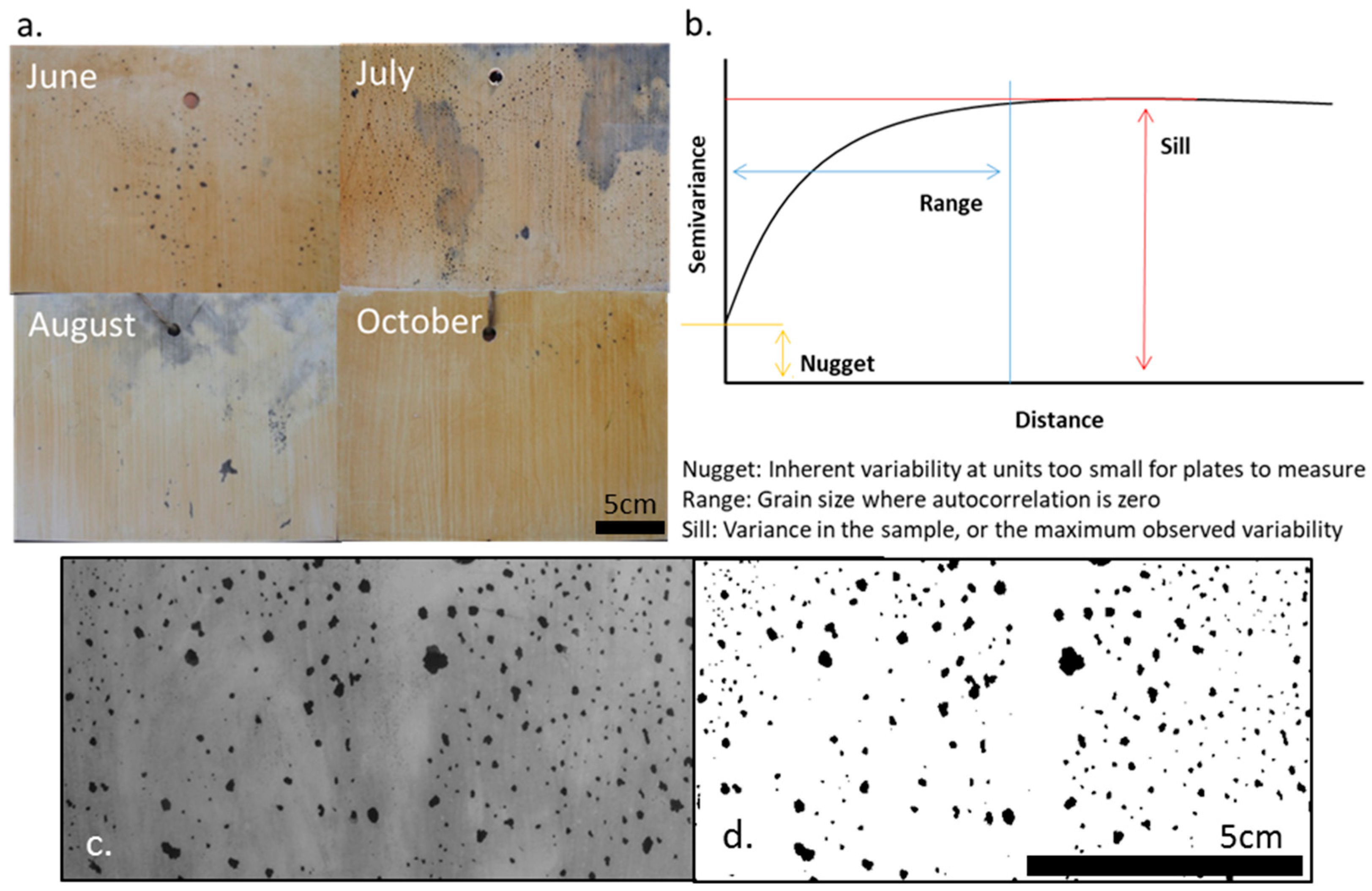
Following numerical analysis, semivariograms of the locations of the black pixels against the white background were constructed in R, using the packages “gstat,”[43] “sp,”[44,45] “plyr,”[46] “dostats,”[47] and “SiZer”[48] (Supporting information R code S1). Using a subset of 5000 random pixels on each plate, five replicate semivariograms were constructed. Five replicate plates were analyzed, for a total of 25 semivariograms per site. From each semivariogram, parameters such as the range, nugget and sill (Figure 2b) were extracted through a looping process in R and the 25 values were averaged into one value for plotting. The top three cm of each plate are described using this method, as additional variation in all parameters was apparent with depth and confounded results.

This process was conducted at four timepoints across the incursion event to effectively create a 4-D map of the belowground FeS characteristics of the wetland (15 cm width and 3 cm depth of the plate in the sediment over a two kilometer transect over time). Of the geostatistical parameters, the nugget (Figure 2b) measures the inherent variability on each plate at short distances [31]. A larger nugget, therefore, indicates more stark differences in color between one spot and another (i.e., the difference between the background white and a distinct black complex as compared to a lower nugget, homogenous plate, either with many complexes or few complexes). The nugget, however, does not indicate the presence or absence of complexes or the number of complexes, rather the change between complex locations at the plate level (Supplemental Information Figure S5).

The range, or grain size, is the lag value at which autocorrelation is zero (Figure 2b). Beyond this distance, there is little to no autocorrelation and values are independent. The sill is the variance in the sample, or the maximum observed variability (Figure 2b). From these, the magnitude of spatial heterogeneity (MSH) can be calculated as the inverse of the relative nugget effect (sill/[sill+nugget]) [49]. This value is zero when there is no spatial heterogeneity (complete homogeneity) and one when the sample is completely heterogeneous [49].

2.5. Relationships between Tranditional Chemistry and IRIS Analysis

We expect traditional soil and porewater chemistry to be related to FeS activity [3]. Iron(II) sulfide precipitation is a function of soil Fe(III) reduction, saltwater-SO₄²⁻ introduction, microbial SO₄²⁻ reduction, and FeS precipitation. Traditional soil and porewater chemistry quantify both the free and aqueous forms of the compounds as well as the solid and precipitated forms of the species. However, not all compounds under consideration are conservative.

For example, Fe(II) is an integral component of FeS. However our quantification methods measure aqueous Fe(II) remaining in the soil porewater, not bound to any constituents [3]. Consequently, the measured quantity is a mirror image of what has precipitated, and thus, we expect an increase in aqueous Fe(II) to be correlated with a decrease in precipitated FeS.

We also predict the SO₄²⁻ concentrations to be time dependent with respect to FeS precipitation; SO₄²⁻ must first reduce to sulfide, then precipitate. Oxidized SO₄²⁻ is predicted to be a mirror image of FeS precipitation as well, as SO₄²⁻ will decrease with reduction and precipitation. However, this can potentially become more complicated with the anticipated SO₄²⁻ pulse travelling through the wetland with overland saltwater incursion, and the non-conservative nature of SO₄²⁻. This could result in no direct relationship between measured SO₄²⁻ and FeS quantification.

We also expect the AVS and CRS measures to be directly correlated to the IRIS plate measures. Both quantify the precipitated and solid phase forms of FeS rather than its aqueous formation components. As such, a more direct comparison should be clear between AVS, CRS, and the IRIS method characterization.

2.6. IRIS Method Advantages and Limitations for Measuring FeS

The field work associated with the IRIS plate method is minimal. The PVC sheets are robust and a mallet can be used to insert the sheets into dense sediment when necessary, although care must be taken to not scratch the FeOOH paint in dry sediments. Two trips to the wetland are needed, however, as the plates require a 24-h incubation. High resolution digital photography is sufficient and digital scanners are not required, unlike similar methods. Additionally, there is no hazardous chemical waste, unlike traditional AVS and CRS techniques. Once cut and sanded, the PVC sheets can be repainted with FeOOH and reused. While there are significant physical advantages to using the modified IRIS method, the greatest advantages are from the new variables that can be assessed. Although a limitation of this method is the lengthy processing time of each photo, pixel and numerical analysis in ImageJ can be streamlined through macros.

Additional considerations during plate photography include consistent lighting which may be difficult depending on cloud cover or flash use. Differences in lighting may incur inaccuracies when determining pixel darkness if the concentration of each FeS compound is being analyzed. One possible solution is photographing against a white background to normalize the white balance of each photograph during the analysis stage. Concentration can be measured on a pixel by pixel basis, as was done here (Supplemental Information Figure S5), however was finally averaged across the entire plate to create one value for reporting in this study. Alternative statistical reporting methods must be employed to represent concentration using the IRIS method.

3. Results

3.1. Soil and Porewater Chemistry

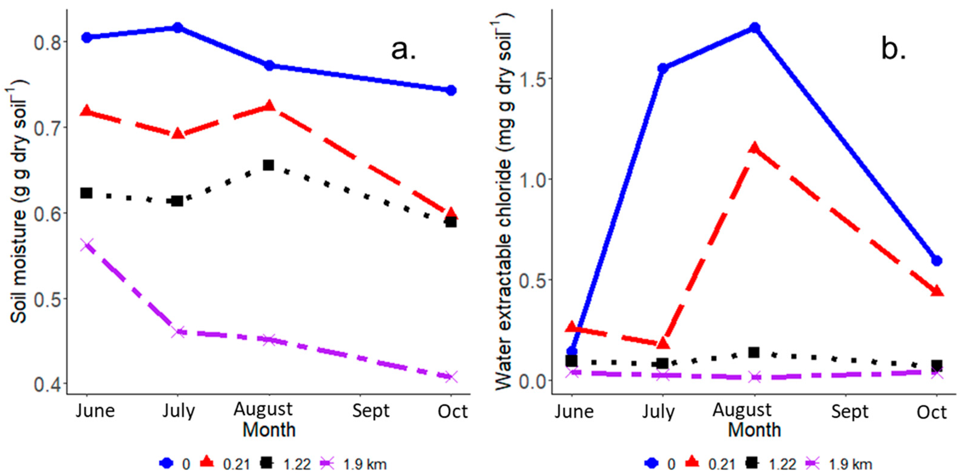
Soil moisture was greatest at the most downstream site (distance = 0 km) at all sampling timepoints. Gravimetric soil moisture content ranged from approximately 80% at the downstream site to approximately 40% at the upstream site, and decreased with distance (Figure 3a).

Water extractable Cl^- was generally greatest at the downstream site (Figure 3b), and also varied with time, peaking in August at ~1.7 mg g⁻¹ dry soil. The Cl^- content peaked in August at the second site around 1.2 mg g⁻¹. Water extractable Cl⁻ at upstream sites (distance > 1 km) varied little over time, remaining <0.25 mg g⁻¹ throughout the saltwater incursion event.

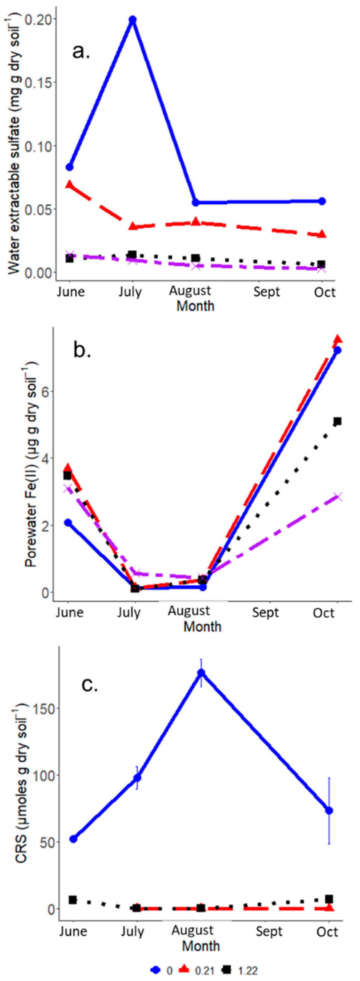
Traditional descriptive measures of FeS activity included water extractable SO₄²⁻, porewater Fe(II), AVS, and CRS. Water extractable SO₄²⁻ varied with distance and time (Figure 4a). Similar to Cl⁻, SO₄^2- was highest in the most downstream site and decreased with distance from this downstream site. However, while Cl⁻ peaked in August, SO₄²⁻ peaked earlier in July. Water extractable SO₄²⁻ reached a maximum of approximately 0.2 mg g⁻¹ in July (Figure 4a).

Porewater Fe(II) concentrations did not follow a similar pattern to water extractable SO₄²⁻ or Cl⁻ concentrations. Rather, they were somewhat mirrored with respect to time. Porewater Fe(II) was between 2 and 4 µg Fe(II) g dry soil⁻¹ in June throughout the site. Concentrations decreased to near the detection limit in July and August, and generally increased to concentrations higher than the pre-incursion levels in October. In October, porewater Fe(II) content was greatest at the two furthest downstream sites with concentrations near 8 µg Fe(II) g dry soil⁻¹ and decreased upstream.

Direct measures of FeS_x formation include AVS and CRS. Measured concentrations of AVS were too low and too variable between replicates and sites to accurately determine patterns amidst large error terms [3]. Chromium reducible sulfur, however, demonstrated clear patterns with distance and time (Figure 4c). By far, the highest CRS values were at the furthest downstream site in August at the peak of the saltwater incursion event, greater than 150 µmoles g dry weight⁻¹. Values were near the detection limit at 1.22 km. Chromium reducible sulfur was not measurable at the most upstream site due to low soil moisture and SO₄²⁻ concentrations.

3.2. IRIS Method Indicators of Altered FeS Activity Across the Saltwater Incursion Gradient

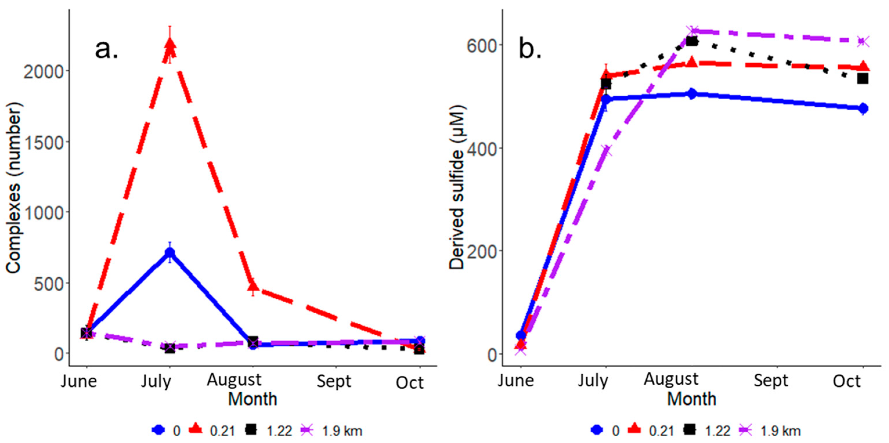
The total number of FeS complexes, derived from IRIS plate quantification, follow a unique pattern in space and time. The greatest number of complexes were not found at the most downstream site, but slightly more inland, at 0.21 km (Figure 5a). This contrasts with the measured SO₄²⁻ and Cl⁻ concentrations. The number of complexes also were greater mid-incursion (July) and decreased at the height of incursion (August). Specifically, the highest number of FeS complexes occur in July at approximately 0.21 km from the downstream outlet, with over 2000 individual complexes. After August and at the freshwater end, the number of complexes decreases rapidly to <500 complexes per 45 cm². The peak in the number of individual FeS complexes occurs while the incursion event intensifies in July, and decreases in August at the peak of the incursion event when water extracted chloride is highest.

The average sulfide concentration (from IRIS-derived FeS complex concentration) of the top three cm of the plate (Figure 5b) was below the detection limit in June (250 µM sulfide) at all sites. The sulfide concentrations during the rest of the saltwater incursion event were much higher but similar across the site (approximately 500–600 µM sulfide). Derived sulfide concentrations also increased further upstream. Thus, the IRIS plate derived sulfide concentration patterns did not directly follow the incursion derived soil and porewater chemistry patterns across space and time.

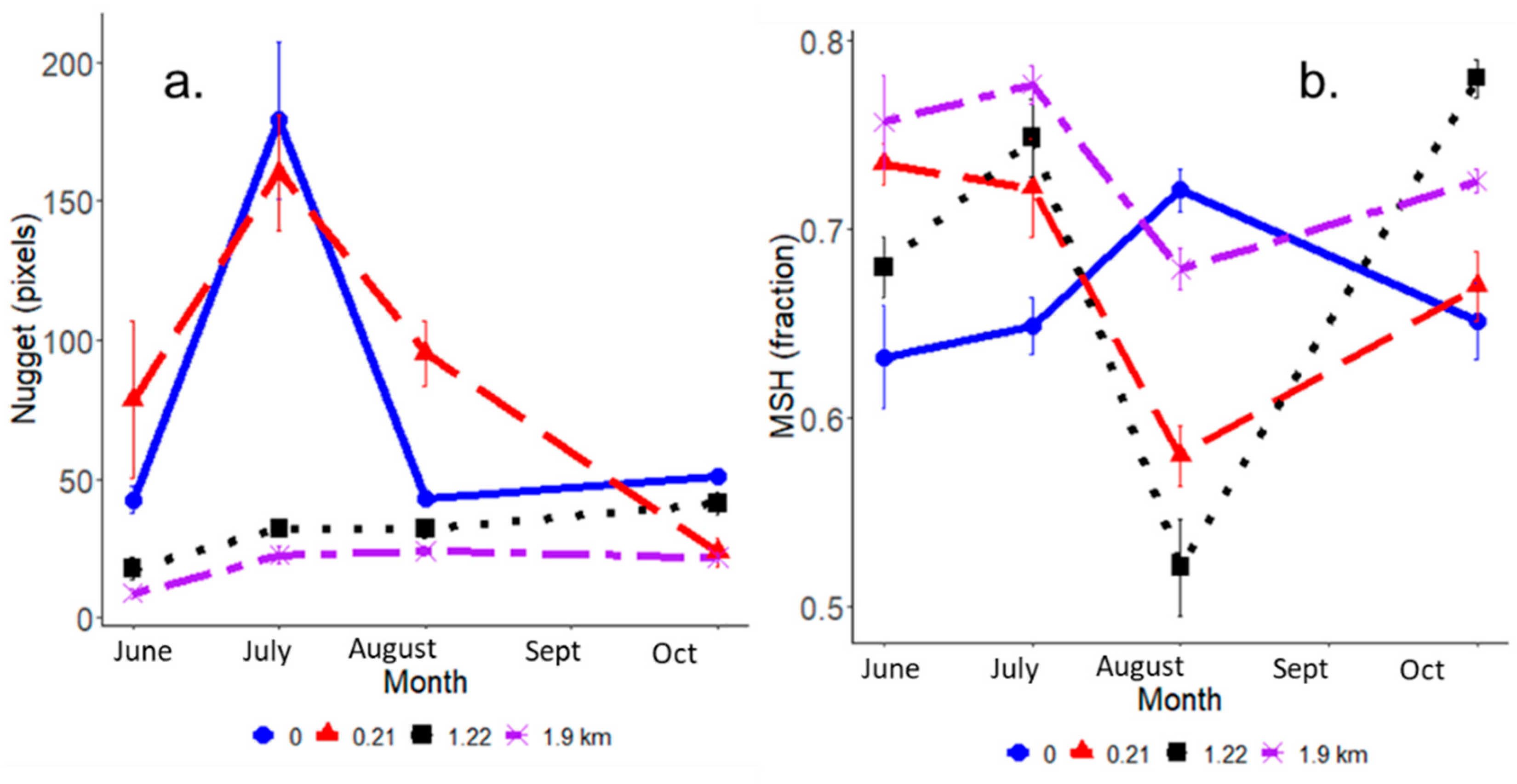
Geostatistical parameters demonstrate distinct zonation by month and distance along the salt-influenced to freshwater gradient. The nugget represents the inherent variability on the site, or the sharp change in complex presence between two sampling points on the same plate (Supplemental Information S3). This was greatest in July at the two most downstream sites (~180 pixels) and this value decreased rapidly with space and time (<50 pixels), following the saltwater pulse (Figure 6a). The Magnitude of Spatial Heterogeneity (MSH) is a summary statistic based on the inverse nugget effect, or the geostatistical parameters of the sill and nugget [49]. Before the incursion event, the farthest downstream site was most homogenous while the inland sites were more heterogeneous (Figure 6b). This trend flipped in August at the height of incursion, with the inland sites more homogenized than the most downstream site.

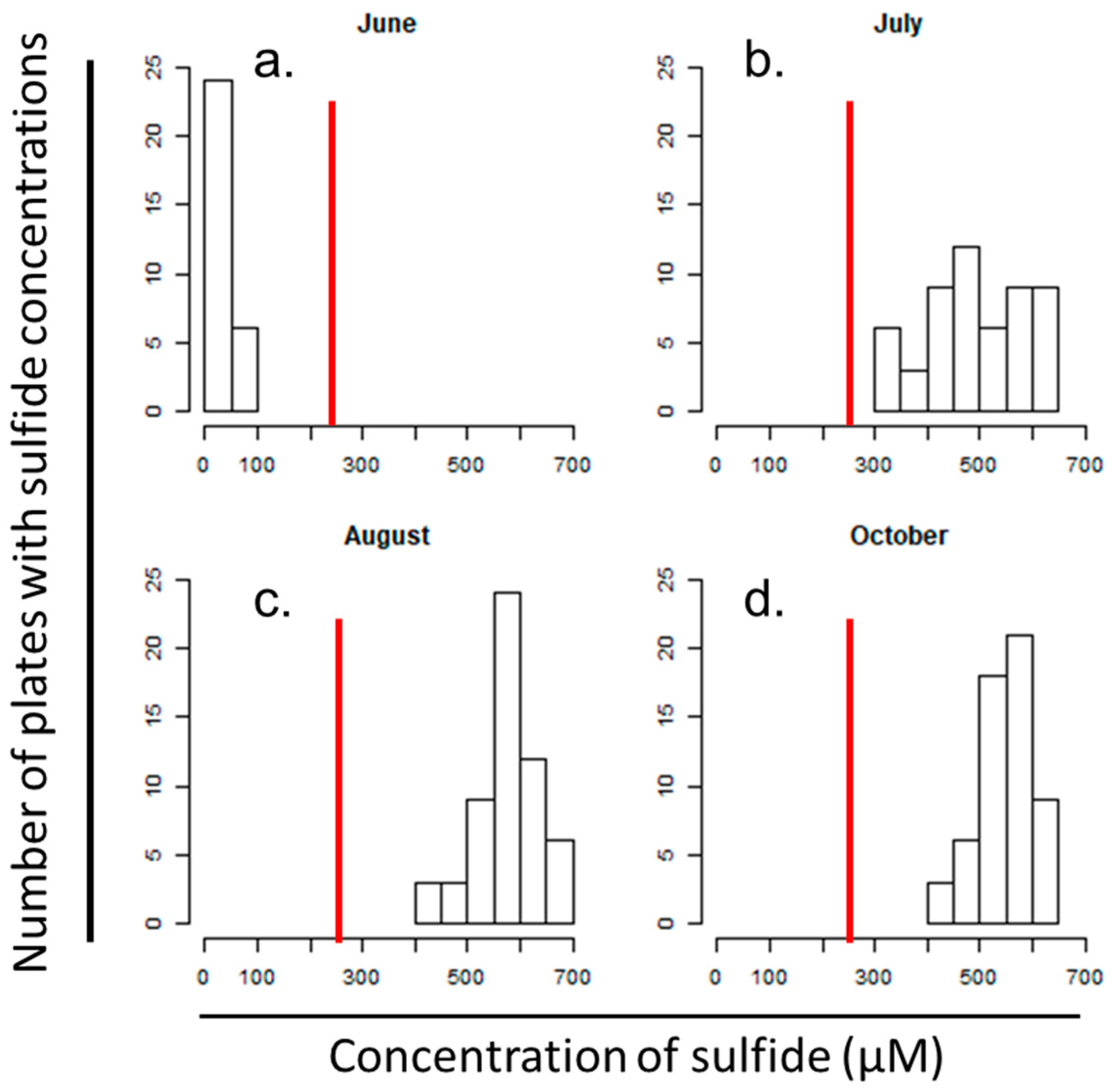
A histogram for each month was created to document the frequency of each plate-averaged concentration found throughout the 25 replicate plates (Figure 7a–d). In June, FeS complexes were visible on some plates, but the concentrations found were below detectable limits (Figure 7a). In July, more derived sulfide was present on the plates (Figure 7b) and the overall number of plates with measurable sulfide concentrations rose. There were higher sulfide concentrations in August (Figure 7c) and October (Figure 7d), with August displaying the highest concentrations.

4. Discussion

4.1. A Saltwater Reaction Front

A reaction front develops within the Timberlake wetland with the progression of saltwater incursion, resulting in gradients in water chemistry both throughout the incursion season and with distance along the wetland. This front moves inland with time and dissipates at the end of the summer season with the seasonal flushing of saltwater by rainfall. The reaction front can be traced through both Cl⁻ (Figure 3b) and SO₄²⁻ concentrations (Figure 4a) in the sediment, which were expected to increase with saltwater incursion [32]. Water extracted Cl⁻ increased in July at the downstream site and remains high through August. At 0.21 km, this pulse is delayed, peaking in August at a lower concentration. Sulfate is typically non-conservative [4] and may be expected to decrease with increased microbial SO₄²⁻ reduction mid-event [3]. Supporting this hypothesis, SO₄²⁻ is highest at the most downstream site in July and decreases drastically in August, at a period of highest SO₄²⁻ reduction rates [3].

The incursion-mediated gradient in SO₄²⁻ concentration is in contrast to the pattern in aqueous Fe(II) concentration found within the sediment porewaters. Iron(III) reduction is the only source of aqueous Fe(II) to the porewaters, and Fe(III), though abundant [3], is still limited in the wetland due to a lack of external input. Consumption of Fe(II) through FeS precipitation then further limits the aqueous Fe(II) available for measurement. Aqueous Fe(II) decreases to near detectable limits in the middle of the incursion event (Figure 4b), likely reflecting this binding of aqueous Fe(II) with reduced sulfide, forming solid phase FeS. As incursion decreases into October and the wetland flushes with freshwater, the sulfides within FeS oxidize first [50], leaving abundant aqueous Fe(II) for measurement (Figure 4b).

The FeS compounds that are hypothesized to form mid-incursion event can potentially be quantified using the AVS and CRS techniques [3,51,52]. While AVS largely quantifies the poorly crystalline and highly reactive FeS compound mackinawite [52], CRS quantifies the more crystalline and stable FeS_x species [52]. Chromium reducible sulfur is most abundant near the downstream site (Figure 4a). Here, there is sufficient sulfide, potentially accumulating over the course of several incursion events, for secondary CRS phases to precipitate. In contrast, AVS concentrations throughout the site were highly variable with up to 40% error between replicate cores [3]. While CRS was a much more reliable measure in this sediment, it does not measure amorphous FeS. Therefore, the uncertainty in AVS concentrations leaves a large gap in our understanding of the dynamic and volatile FeS compounds throughout the incursion event.

4.2. Detailed View of Heterogeneity Parameters under Heavy Salt Water Influence

The nugget parameter is expected to be lower both with low and high sea salts, indicating more uniformity in the presence or absence of complexes. The larger nuggets were found following the initial inward pulse of saltwater (i.e., in July during the most dynamic period of sea salt change) but not after July, suggesting the introduction of saltwater is related to spatial heterogeneity of the FeS complexes. However, the nugget parameter alone does not provide a complete view of the trends.

July and August display vastly different responses in the water extracted SO₄²⁻ concentration, the number of complexes, and the MSH, especially when comparing the first and second sites (i.e., those sites and months most heavily influenced by saltwater incursion). For example, when observing the most downstream site (0 km), the water extracted SO₄²⁻ is highest in July (Figure 4a). Schoepfer et al. [3] document the highest SO₄²⁻ reduction rates at this site in August, however, suggesting SO₄²⁻ reduction largely consumes the available SO₄²⁻ in August, removing it from the measurable pool and yielding lower available SO₄²⁻ concentrations.

We can hypothesize that the SO₄²⁻ content and the number of FeS complexes are related. However, the relationship between space, time, SO₄²⁻, and the number of complexes is much more dynamic. At 0 km, the most complexes are found in July (Figure 5a), which may reflect the increased available SO₄²⁻ from salt water incursion (Figure 4a). However, the second site (0.21 km) had a greater number of complexes than the first site in July despite lower extractable SO₄²⁻ content. The higher number of complexes is likely related to decreased soil moisture at this second site in the transect (Figure 3a), rather than SO₄²⁻ content. This assertion is supported by the average area per complex (Supplemental information Figure S4). The relationship between the number of pixels, distance, and month suggests that the largest complexes at 0 km were found in August at the height of incursion and decreased with the flushing of salt water by freshwater. The largest complexes at the second site (0.21 km) were found later, in October. We hypothesize that decreased soil moisture at 0.21 km isolates the drier soil particles and associated SO₄²⁻ until later in the season. In contrast, higher soil moisture at the first site may spread out and dilute the SO₄²⁻ and subsequent FeS in the soil profile in August [13,53,54,55]. The increased dilution at the first site may explain the fewer number of complexes (i.e., fewer but larger and more connected complexes at 0 km).

Soil moisture alone does not explain the trends in the MSH in August, where the first site (0 km) has the highest MSH. Homogeneity was thought to be limited by soil moisture in July, but the CRS content may be influencing the MSH as well, especially later in the season. The number of individual FeS complexes at the first site in August is substantially lower than in July. The IRIS based FeS measurements only document the amorphous, poorly crystalline sulfide minerals and does not document any crystallization of these minerals to FeS_x, which can occur with the addition of extra sulfide [56,57]. However, CRS measures this more crystalline fraction of reduced inorganic sulfur minerals [58] and peaks in August at the first site (Figure 4c). It is possible, therefore, that this first site has accumulated enough sulfide to transition from an AVS dominated system (amorphous and poorly crystalline FeS species) [51] to a CRS dominated system (crystalline FeS_x) and the IRIS plates are not able to measure this transition [24]. Therefore, the remaining AVS on the plate may be more heterogeneous when compared to the second site due to selective or perhaps random crystallization. Acid volatile sulfide was determined in these locations [3], however had up to 40% error at each site, which restricted the reliability of the data. Future work could include the use of portable x-ray fluorescence, used to scan and map the chemical and elemental composition on the IRIS plate, including those pixels that have transitioned from amorphous to crystalline FeS_x.

In contrast, the second site (0.21 km) becomes more homogeneous in August and may be a function of the reaction front moving inland or less buildup of sulfide over the years, resulting in more amorphous, AVS-measurable FeS visible on the plates. However, despite differences in the MSH, all values were indicative of more heterogeneity than homogeneity (values > 0.5), suggesting the larger wetland is only marginally influenced by saltwater incursion. This conclusion supports Schoepfer et al. [3], who conclude the presence of an iron-clad wetland that will buffer against the seawater-SO₄²⁻ input for many more years. We hypothesize that with additional SO₄²⁻ (either through larger or longer incursion events), soils will become more homogenous with respect to FeS as the small and dark complexes currently present become larger and merge, to eventually occupy the entire sediment profile.

In support of this projection, we can see the most upstream site (1.9 km) had a relatively high MSH (around or above 0.7), indicating high heterogeneity in the absence of increased salt water. This may be due to both the low soil moisture at the upstream site and low SO₄²⁻ content of that incoming water. Together, the lack of water and lack of SO₄²⁻ result in a patchy FeS soil profile where the low concentrations of SO₄²⁻ cannot be united in the pore spaces to create larger and more uniformly distributed complexes [13,59,60,61].

In summary, both increased soil moisture and elevated sea salts are suspected to be the driving factor in determining FeS complex formation and subsequent homogeneity. Waterlogging of sediments with SO₄²⁻ rich water both supplies the necessary SO₄²⁻ for microbial SO₄²⁻ reduction and unifies soil pores, therefore more evenly redistributing resources [13,59,60,61]. The summary statistic of the MSH demonstrates this homogenization of the FeS complexes within the soil profile over the course of the summer incursion event using the IRIS method at the three inland sites. The most downstream site, however, is influenced by the excess sulfide precipitation as CRS species, possibly due to seasonally repeated incursion cycles. As such, the IRIS method is limited in its robustness until further statistical measures are refined to determine sulfide concentration on a pixel by pixel basis (See Supplemental Information Figure S5).

4.3. IRIS Method Determination of FeS Concentrations

Rabenhorst et al. [24] developed a method to determine sulfide concentrations on IRIS plates. Using this method, average sulfide concentrations across the entire 3 × 15 cm section of the plate were determined. We hypothesize that the larger complexes would be lighter in color due to dilution. However, the quantitative values determined via this method (Figure 5b) were not representative of the qualitative visual analyses. Furthermore, a large amount of detail was lost in the averaging process. For example, the larger complexes were visually often lighter in color than the more numerous smaller complexes (Figure 2a). However, the IRIS derived sulfide concentrations were similar across site and time following salt water incursion, as most distance and time related trends were eliminated through averaging, representing a uniform, higher concentration throughout space and time (Figure 5b).

To further distinguish the derived sulfide concentrations among months, a histogram function was used (Figure 7). This method took the average concentration per plate for each of 25 replicates throughout the four sites. Despite sites being grouped in this analysis, August displays the greatest number of plates with higher sulfide concentrations when compared to June, July and October. Increased sulfide in August supports our hypothesis that August was the height of the incursion season even though water extracted SO₄²⁻ was low. Increased SO₄²⁻ reduction was not discernable when averaging the entire plate sulfide concentrations, suggesting much more work into the statistical background of the complex location and concentration is needed. Furthermore, although complexes were detectable in June, the sulfide concentrations were too low for accurate analysis. Consequently, the use of the IRIS plate method may be limited in low sulfide locations and must be paired with traditional bulk chemical analyses in freshwater sites.

5. Conclusions

Here, we have slightly modified the IRIS technique and introduced new quantification methods for FeS identification in wetland sediments. We show how (1) FeS spatial heterogeneity is present in a fresh-to-brackish transitioning wetland, and (2) how increased salt water input altered this heterogeneity, specifically with regard to the SO₄²⁻ input to the wetland. Other factors that may play an important role in the differences in the MSH are the CRS concentrations, the SO₄²⁻ reducing bacteria pool [59,60] and the hydrology on the site [61,62], all which influence amorphous (IRIS measurable) FeS complex formation. Although the hydrology at the site has been described previously [33,34], integration of hydrology with the modified IRIS method will likely aid in our understanding of belowground FeS patterns and our predictive abilities of FeS characteristics.

The presence of FeS largely controls acidity dynamics [6] as well as nutrient and contaminant sorption and mobility [7,8]. A more homogeneous sediment may be able to more uniformly retain metals and nutrients sorbed to the FeS structure, naturally mitigating the coastlines against excess waste-containing material (i.e., agricultural or industrial runoff). However, a freshwater wetland experiencing only some saltwater incursion (i.e., high heterogeneity) may not be able to consistently buffer the surrounding waters against pollutants. Therefore, although sulfidization of the sediment is not a threat in these particular fresh-to-brackish transitioning sediments [3], the pH dynamics during repeated flooding and drying events (and subsequent reduction and oxidation of FeS) [9] must be monitored, as well as the metal and nutrient mobility resulting from potential changes in pH.

Future work into the development of this method should focus on streamlining the plate analysis procedure. The process of transforming photos to coordinates and greyscale values is not difficult in ImageJ, however is time consuming. As a result, the rate limiting step in the analysis procedure is the hand extraction of individual plate coordinate data from ImageJ to a data management software. If this process can be automated through the use of macros, the spatial analysis of the photos will be greatly streamlined. Furthermore, alternative statistical methods (i.e., detailed histogram analysis or spot-by-spot analysis of FeS complex sulfide concentrations) will greatly enhance the IRIS method and provide a more direct comparison to traditional AVS and CRS measurements.

References

- Hines, M.M.E.M.; Knollmeyer, S.S.L.S.; Tugel, J.; Tugei, J.B.; Tugel, J. Sulfate reduction and other sedimentary biogeochemistry in a northern New England salt marsh. Limnol. Oceanogr. 1989, 34, 578–590. [Google Scholar] [CrossRef] [Green Version]
- Weston, N.B.; Dixon, R.E.; Joye, S.B. Ramifications of increased salinity in tidal freshwater sediments: Geochemistry and microbial pathways of organic matter mineralization. J. Geophys. Res. 2006, 111, 1–14. [Google Scholar] [CrossRef]
- Schoepfer, V.A.; Bernhardt, E.S.; Burgin, A.J. Iron clad wetlands: Soil iron-sulfur buffering determines coastal wetland response to salt water incursion. J. Geophys. Res. Biogeosci. 2014, 119, 2209–2219. [Google Scholar] [CrossRef] [Green Version]
- Van Dijk, G.; Smolders, A.J.P.; Loeb, R.; Bout, A.; Roelofs, J.G.M.; Lamers, L.P.M. Salinization of coastal freshwater wetlands; effects of constant versus fluctuating salinity on sediment biogeochemistry. Biogeochemistry 2015, 126, 71–84. [Google Scholar] [CrossRef]
- Herbert, E.R.; Boon, P.; Burgin, A.J.A.J.; Neubauer, S.C.S.C.; Franklin, R.B.R.B.; Ardón, M.; Hopfensperger, K.N.; Lamers, L.P.M.; Gell, P.; Ardon, M.; et al. A global perspective on wetland salinization: Ecological consequences of a growing threat to freshwater wetlands. Ecosphere 2015, 6, art206. [Google Scholar] [CrossRef]
- Burton, E.D.; Bush, R.T.; Sullivan, L.A.; Hocking, R.K.; Mitchell, D.R.G.; Johnston, S.G.; Fitzpatrick, R.W.; Raven, M.; McClure, S.; Jang, L.Y. Iron-Monosulfide Oxidation in Natural Sediments: Resolving Microbially Mediated S Transformations Using XANES, Electron Microscopy, and Selective Extractions. Environ. Sci. Technol. 2009, 43, 3128–3134. [Google Scholar] [CrossRef]
- Gao, Y.; van de Velde, S.; Williams, P.N.; Baeyens, W.; Zhang, H. Two-dimensional images of dissolved sulfide and metals in anoxic sediments by a novel diffusive gradients in thin film probe and optical scanning techniques. TrAC Trends Anal. Chem. 2015, 66, 63–71. [Google Scholar] [CrossRef]
- Niazi, N.K.; Burton, E.D. Arsenic sorption to nanoparticulate mackinawite (FeS): An examination of phosphate competition. Environ. Pollut. 2016, 218, 111–117. [Google Scholar] [CrossRef] [PubMed]
- Karimian, N.; Johnston, S.G.; Burton, E.D. Effect of cyclic redox oscillations on water quality in freshwater acid sulfate soil wetlands. Sci. Total Environ. 2017, 581–582, 314–327. [Google Scholar] [CrossRef] [PubMed]
- Borch, T.; Kretzschmar, R.; Kappler, A.; Cappellen, P.V.; Ginder-Vogel, M.; Voegelin, A.; Campbell, K. Biogeochemical Redox Processes and their Impact on Contaminant Dynamics. Environ. Sci. Technol. 2010, 44, 15–23. [Google Scholar] [CrossRef] [PubMed]
- Burton, E.D.; Sullivan, L.A.; Bush, R.T.; Johnston, S.G.; Keene, A.F. A simple and inexpensive chromium-reducible sulfur method for acid-sulfate soils. Appl. Geochem. 2008, 23, 2759–2766. [Google Scholar] [CrossRef]
- Kefi, S.; Guttal, V.; Brock, W.A.; Carpenter, S.R.; Ellison, A.M.; Livina, V.N.; Seekell, D.A.; Scheffer, M.; Van Nes, E.H.; Dakos, V.; et al. Early warning signals of ecological transitions: Methods for spatial patterns. PLoS ONE 2014, 9, 10–13. [Google Scholar] [CrossRef] [PubMed]
- Santner, J.; Larsen, M.; Kreuzeder, A.; Glud, R.N. Two decades of chemical imaging of solutes in sediments and soils—A review. Anal. Chim. Acta 2015, 878, 9–42. [Google Scholar] [CrossRef] [PubMed]
- Johnston, S.G.; Burton, E.D.; Aaso, T.; Tuckerman, G. Sulfur, iron and carbon cycling following hydrological restoration of acidic freshwater wetlands. Chem. Geol. 2014, 371, 9–26. [Google Scholar] [CrossRef]
- Ettema, C.H.; Wardle, D.A. Spatial soil ecology. Trends Ecol. Evol. 2002, 17, 177–183. [Google Scholar] [CrossRef]
- Bennett, W.W.; Teasdale, P.R.; Welsh, D.T.; Panther, J.G.; Jolley, D.F. Optimization of colorimetric DET technique for the in situ, two-dimensional measurement of iron(II) distributions in sediment porewaters. Talanta 2012, 88, 490–495. [Google Scholar] [CrossRef] [PubMed]
- Stockdale, A.; Davison, W.; Zhang, H. Micro-scale biogeochemical heterogeneity in sediments: A review of available technology and observed evidence. Earth-Sci. Rev. 2009, 92, 81–97. [Google Scholar] [CrossRef] [Green Version]
- Robertson, D.; Welsh, D.T.; Teasdale, P.R. Investigating biogenic heterogeneity in coastal sediments with two-dimensional measurements of iron(II) and sulfide. Environ. Chem. 2009, 6, 60–69. [Google Scholar] [CrossRef]
- Viollier, E.; Rabouille, C.; Apitz, S.E.; Breuer, E.; Chaillou, G.; Dedieu, K.; Furukawa, Y.; Grenz, C.; Hall, P.; Janssen, F.; et al. Benthic biogeochemistry: State of the art technologies and guidelines for the future of in situ survey. J. Exp. Mar. Biol. Ecol. 2003, 285–286, 5–31. [Google Scholar] [CrossRef]
- Gao, Y.; Leermakers, M.; Elskens, M.; Billon, G.; Ouddane, B.; Fischer, J.C.; Baeyens, W. High resolution profiles of thallium, manganese and iron assessed by DET and DGT techniques in riverine sediment pore waters. Sci. Total Environ. 2007, 373, 526–533. [Google Scholar] [CrossRef]
- Vandenhove, H.; Antunes, K.; Wannijn, J.; Duquène, L.; Van Hees, M. Method of diffusive gradients in thin films (DGT) compared with other soil testing methods to predict uranium phytoavailability. Sci. Total Environ. 2007, 373, 542–555. [Google Scholar] [CrossRef] [PubMed]
- Wu, Z.; Wang, S.; Jiao, L.; Wu, F. The simultaneous measurement of phosphorus, sulfide, and trace metals by ferrihydrite/AgI/Chelex-100 DGT (diffusive gradients in thin films) Probe at sediment/water interface (SWI) and remobilization assessment. Water Air Soil Pollut. 2014, 225. [Google Scholar] [CrossRef]
- Neubauer, S.C.; Anderson, I.C.; Neikirk, B.B. Nitrogen cycling and ecosystem exchanges in a Virginia tidal freshwater marsh. Estuaries 2005, 28, 909–922. [Google Scholar] [CrossRef]
- Rabenhorst, M.C.; Megonigal, J.P.; Keller, J. Synthetic Iron Oxides for Documenting Sulfide in Marsh Pore Water. Soil Sci. Soc. Am. J. 2010, 74, 1383. [Google Scholar] [CrossRef]
- Rabenhorst, M.C. A System for Making and Deploying Oxide-Coated Plastic Films for Environmental Assessment of Soils. Soil Sci. Soc. Am. J. 2018, 82, 1301. [Google Scholar] [CrossRef]
- Rabenhorst, M.C.; Burch, S.N. Synthetic Iron Oxides as an Indicator of Reduction in Soils (IRIS). Soil Sci. Soc. Am. J. 2006, 70, 1227. [Google Scholar] [CrossRef]
- Rabenhorst, M.C. Visual Assessment of IRIS Tubes in Field Testing for Soil Reduction. Wetlands 2010, 30, 847–852. [Google Scholar] [CrossRef]
- Vaness, B.M.; Wilson, S.D.; Macdougall, A.S. Decreased root heterogeneity and increased root length following grassland invasion. Funct. Ecol. 2014, 28, 1266–1273. [Google Scholar] [CrossRef] [Green Version]
- Zuo, X.A.; Zhao, X.Y.; Zhao, H.L.; Guo, Y.R.; Zhang, T.H.; Cui, J.Y. Spatial pattern and heterogeneity of soil organic carbon and nitrogen in sand dunes related to vegetation change and geomorphic position in Horqin Sandy Land, Northern China. Environ. Monit. Asses. 2010, 164, 29–42. [Google Scholar] [CrossRef]
- Lin, Y.; Hong, M.; Han, G.; Zhao, M.; Bai, Y.; Chang, S.X. Grazing intensity affected spatial patterns of vegetation and soil fertility in a desert steppe. Agric. Ecosyst. Environ. 2010, 138, 282–292. [Google Scholar] [CrossRef]
- Schlesinger, W.H.; Raikes, J.A.; Hartley, A.E.; Cross, A.F. On the Spatial Pattern of Soil Nutrients in Desert Ecosystems. Ecology 1996, 77, 364–374. [Google Scholar] [CrossRef]
- Ardón, M.; Morse, J.L.; Colman, B.P.; Bernhardt, E.S. Drought-induced saltwater incursion leads to increased wetland nitrogen export. Glob. Chang. Biol. 2013, 19, 2976–2985. [Google Scholar] [CrossRef]
- Ardón, M.; Montanari, S.; Morse, J.L.; Doyle, M.W.; Bernhardt, E.S. Phosphorus export from a restored wetland ecosystem in response to natural and experimental hydrologic fluctuations. J. Geophys. Res. 2010, 115. [Google Scholar] [CrossRef] [Green Version]
- Morse, J.L.; Ardón, M.; Bernhardt, E.S. Greenhouse gas fluxes in southeastern U.S. coastal plain wetlands under contrasting land uses. Ecol. Appl. 2012, 22, 264–280. [Google Scholar] [CrossRef] [Green Version]
- Helton, A.M.; Bernhardt, E.S.; Fedders, A. Biogeochemical regime shifts in coastal landscapes: The contrasting effects of saltwater incursion and agricultural pollution on greenhouse gas emissions from a freshwater wetland. Biogeochemistry 2014, 120, 133–147. [Google Scholar] [CrossRef]
- Ardón, M.; Helton, A.M.; Scheuerell, M.D.; Bernhardt, E.S. Fertilizer legacies meet saltwater incursion: Challenges and constraints for coastal plain wetland restoration. Elem. Sci. Anth. 2017, 5, 41. [Google Scholar] [CrossRef]
- Ardón, M.; Morse, J.L.; Doyle, M.W.; Bernhardt, E.S. The Water Quality Consequences of Restoring Wetland Hydrology to a Large Agricultural Watershed in the Southeastern Coastal Plain. Ecosystems 2010, 13, 1060–1078. [Google Scholar] [CrossRef]
- Neubauer, S.C.; Givler, K.; Valentine, S.S.; Megonigal, J.P. Seasonal Patterns and Plant-Mediated Controls of Subsurface Wetland Biogeochemistry. Ecology 2005, 86, 3334–3344. [Google Scholar] [CrossRef]
- Fossing, H.; Jørgensen, B.B. Measurement of bacterial sulfate reduction in sediments: Evaluation of a single-step chromium reduction method. Biogeochemistry 1989, 8, 205–222. [Google Scholar] [CrossRef]
- Allen, H.E.; Fu, G.; Deng, B. Analysis of acid volatile sulfide (AVS) and simultaneously extracted metals (SEM) for the estimation of potential toxicity in aquatic sediments. Environ. Toxicol. Chem. 1993, 12, 1441–1453. [Google Scholar] [CrossRef]
- Jenkinson, B.J.; Franzmeier, D.P. Development and Evaluation of Iron-Coated Tubes that Indicate Reduction in Soils. Soil Sci. Soc. Am. J. 2006, 70, 183. [Google Scholar] [CrossRef]
- Rasband, W.S. ImageJ; U. S. National Institutes of Health: Bethesda, MD, USA, 1997.
- Pebesma, E. Spatio-temporal geostatistics using gstat. Available online: http://citeseerx.ist.psu.edu/viewdoc/download?doi=10.1.1.432.106&rep=rep1&type=pdf (accessed on 31 March 2019).
- Pebesma, E.; Bivand, R.S.S. Classes and Methods for Spatial Data: The sp Package. R News 5 (2). 2005, pp. 1–21. Available online: https://cran.r-project.org/doc/Rnews/ (accessed on 31 March 2019).
- Bivand, R.S.; Pebesma, E.J.; Gomez-Rubio, V. Applied Spatial Data Analysis with R, 2nd ed.; Springer: New York, NY, USA, 2013. [Google Scholar]
- Wickham, H. The Split-Apply-Combine Strategy for Data Analysis. J. Stat. Softw. 2011, 40, 1–29. [Google Scholar] [CrossRef]
- Redd, A. Dostats: Compute Statistics Helper Functions. 2015, pp. 1–13. Available online: https://github.com/halpo/dostats (accessed on 31 March 2019).
- Sonderegger, D. SiZer: SiZer: Significant Zero Crossings. 2015, pp. 1–15. Available online: https://github.com/dereksonderegger/SiZer (accessed on 31 March 2019).
- Lane, D.R.; BassiriRad, H. Diminishing Spatial Heterogeneity in Soil Organic Matter across a Prairie Restoration Chronosequence. Restor. Ecol. 2005, 13, 403–412. [Google Scholar] [CrossRef]
- Paul, S.; Kusel, K.; Alewell, C. Reduction processes in forest wetlands: Tracking down heterogeneity of source/sink functions with a combination of methods. Soil Biol. Biochem. 2006, 38, 1028–1039. [Google Scholar] [CrossRef]
- Rickard, D.; Morse, J.W. Acid volatile sulfide (AVS). Mar. Chem. 2005, 97, 141–197. [Google Scholar] [CrossRef]
- Burton, E.D.; Bush, R.T.; Sullivan, L.A. Sedimentary iron geochemistry in acidic waterways associated with coastal lowland acid sulfate soils. Geochim. Cosmochim. Acta 2006, 70, 5455–5468. [Google Scholar] [CrossRef]
- Orr, C.H.; Predick, K.I.; Stanley, E.H.; Rogers, K.L. Spatial autocorrelation of denitrification in a restored and a natural floodplain. Wetlands 2014, 34, 89–100. [Google Scholar] [CrossRef]
- Harms, T.K.; Wentz, E.A.; Grimm, N.B. Spatial heterogeneity of denitrification in semi-arid floodplains. Ecosystems 2009, 12, 129–143. [Google Scholar] [CrossRef]
- Ekschmitt, K.; Kandeler, E.; Poll, C.; Brune, A.; Buscot, F.; Friedrich, M.; Gleixner, G.; Hartmann, A.; Kästner, M.; Marhan, S.; et al. Soil-carbon preservation through habitat constraints and biological limitations on decomposer activity. J. Plant Nutr. Soil Sci. 2008, 171, 27–35. [Google Scholar] [CrossRef]
- Kraal, P.; Burton, E.D.; Bush, R.T. Iron monosulfide accumulation and pyrite formation in eutrophic estuarine sediments. Geochim. Cosmochim. Acta 2013, 122, 75–88. [Google Scholar] [CrossRef]
- Burton, E.D.; Bush, R.; Sullivan, L. Fractionation and extractability of sulfur, iron and trace elements in sulfidic sediments. Chemosphere 2006, 64, 1421–1428. [Google Scholar] [CrossRef]
- Kallmeyer, J.; Ferdelman, T.G.; Weber, A.; Fossing, H.; Jørgensen, B.B. A cold chromium distillation procedure for radiolabeled sulfide applied to sulfate reduction measurements: Sulfate reduction cold Cr-II method. Limnol. Oceanog. Methods 2004, 2, 171–180. [Google Scholar] [CrossRef]
- Concostrina-Zubiri, L.; Huber-Sannwald, E.; Martínez, I.; Flores Flores, J.L.; Escudero, A. Biological soil crusts greatly contribute to small-scale soil heterogeneity along a grazing gradient. Soil Biol. Biochem. 2013, 64, 28–36. [Google Scholar] [CrossRef]
- Jackson, R.B.; Caldwell, M. Geostatistical patterns of soil heterogeneity around individual perennial plants. J. Ecol. 1993, 81, 683–692. [Google Scholar] [CrossRef]
- Burt, T.P.; Matchett, L.S.; Goulding, K.W.T.; Webster, C.P.; Haycock, N.E. Denitrification in riparian buffer zones: The role of floodplain hydrology. Hydrol. Process. 1999, 13, 1451–1463. [Google Scholar] [CrossRef]
- Burt, T.P.; Pinay, G. Linking hydrology and biogeochemistry in complex landscapes. Progr. Phys. Geogr. 2005, 29, 297–316. [Google Scholar] [CrossRef]
Figure 1.
Map of sampling locations (colored shapes) along the salt-influenced downstream (northern end) to largely freshwater upstream (southern end) two kilometer transect. Freshwater flows south to north, while saltwater incursion pushes inland north to south. Insert depicts the specific conductivity of surface water (light blue circles = downstream site, purple crosses = upstream site) over the year [3]. The sampling dates are indicated by grey vertical lines.
Figure 2.
(a) Representative IRIS plates at each sampling date. FeS appears as black complexes, either discretely or as aggregated units. (b) A model semivariogram and the variables extracted. And, a raw plate showing FeS complexes transformed to (c) greyscale and (d) black and white.
Figure 3.
(a) Gravimetric soil moisture (g water g dry soil−1) and (b) Water extractable Cl− (mg Cl− g dry soil−1) with distance from the most downstream site (km) per month (June-October).
Figure 4.
(a) Water extractable SO42− (mg g dry soil−1), (b) Fe(II) (µg Fe(II) g dry soil−1), and (c) chromium reducible sulfur (CRS, µmoles g dry soil−1) versus distance from the downstream site (km) and through time (month). Error bars denote standard errors.
Figure 5.
IRIS plate derived patterns in (a) the number of complexes per 45 cm2 and (b) the calculated sulfide concentration (µM sulfide) averaged across each plate across wetland distance (km) and per month. Values are an average across the total 3 × 15 cm plate, averaging all white, grey, and black spaces. Error bars denote standard errors.
Figure 6.
IRIS derived patterns in the (a) nugget (pixels) and in the (b) fractional value of the magnitude of spatial heterogeneity across distance in the wetland (km) and by month. Nugget values are calculated as a mean of 25 replicate semivariograms from each site and depth. The MSH is a summary statistic based off the geostatistical parameters. When the MSH equals 1, the site is completely heterogeneous. Error bars denote standard errors.
Figure 7.
IRIS plate derived sulfide concentrations across site for each month throughout the incursion season. The frequency of each plate-averaged concentration is displayed on the y axis and the average concentration per plate is binned on the x axis in (a) June, (b) July, (c) August, and (d) October. Red vertical lines denote the detection limit of derived sulfide. Values below this limit indicate that FeS complexes were present, but concentration values are not reliable. Sulfide concentrations represent the average of each white, grey, and black pixel on the plate.
© 2019 by the authors. Licensee MDPI, Basel, Switzerland. This article is an open access article distributed under the terms and conditions of the Creative Commons Attribution (CC BY) license (http://creativecommons.org/licenses/by/4.0/).
Share and Cite
MDPI and ACS Style
Schoepfer, V.A.; Burgin, A.J.; Loecke, T.D.; Helton, A.M. Seasonal Salinization Decreases Spatial Heterogeneity of Sulfate Reducing Activity. Soil Syst. 2019, 3, 25. https://doi.org/10.3390/soilsystems3020025
AMA Style
Schoepfer VA, Burgin AJ, Loecke TD, Helton AM. Seasonal Salinization Decreases Spatial Heterogeneity of Sulfate Reducing Activity. Soil Systems. 2019; 3(2):25. https://doi.org/10.3390/soilsystems3020025
Chicago/Turabian StyleSchoepfer, Valerie A., Amy J. Burgin, Terry D. Loecke, and Ashley M. Helton. 2019. "Seasonal Salinization Decreases Spatial Heterogeneity of Sulfate Reducing Activity" Soil Systems 3, no. 2: 25. https://doi.org/10.3390/soilsystems3020025