
A Classification Method of Point Clouds of Transmission Line Corridor Based on Improved Random Forest and Multi-Scale Features
 ,
,
Abstract
:1. Introduction
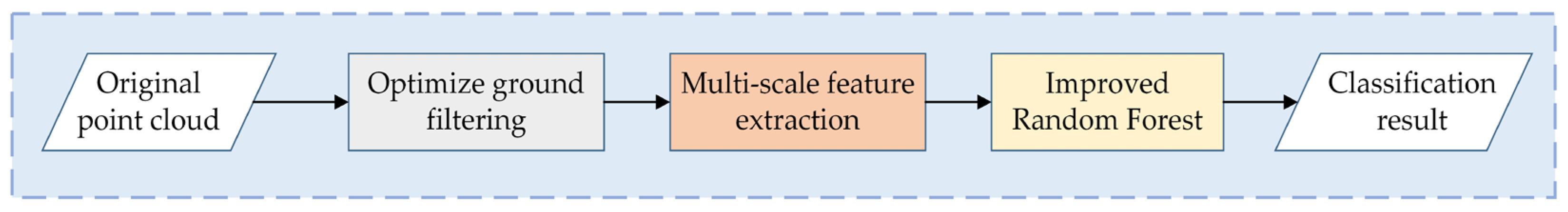
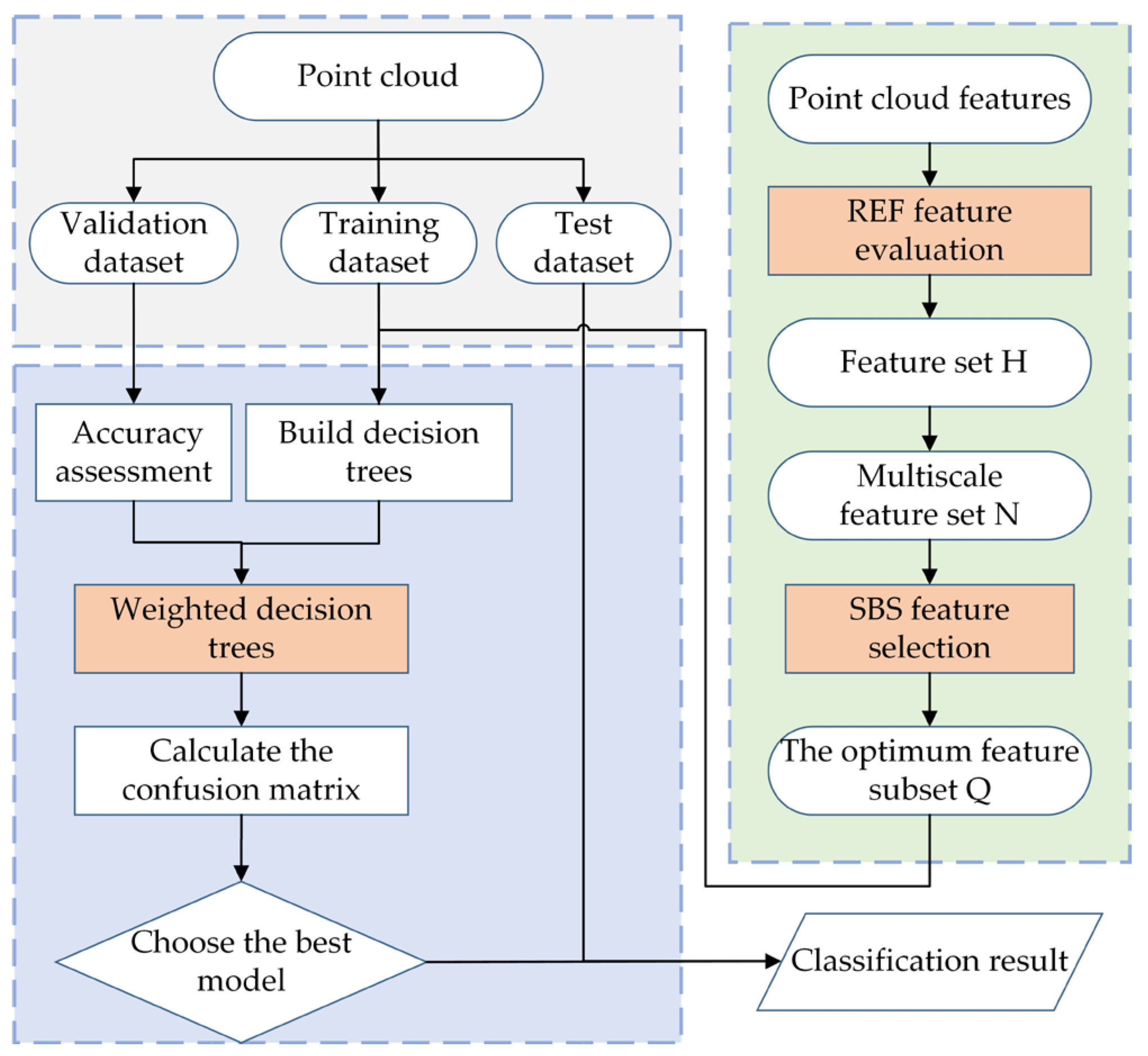
2. Method
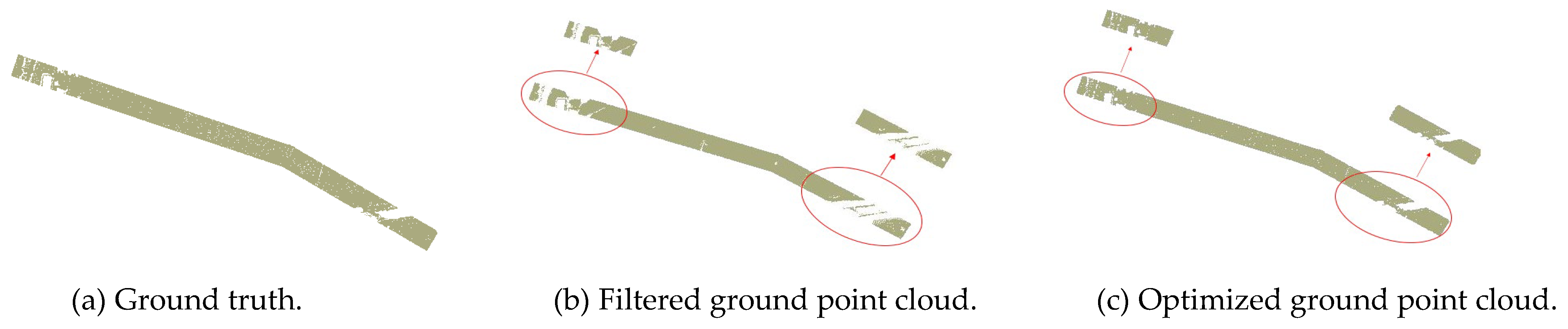
2.1. Ground Point Cloud Filter
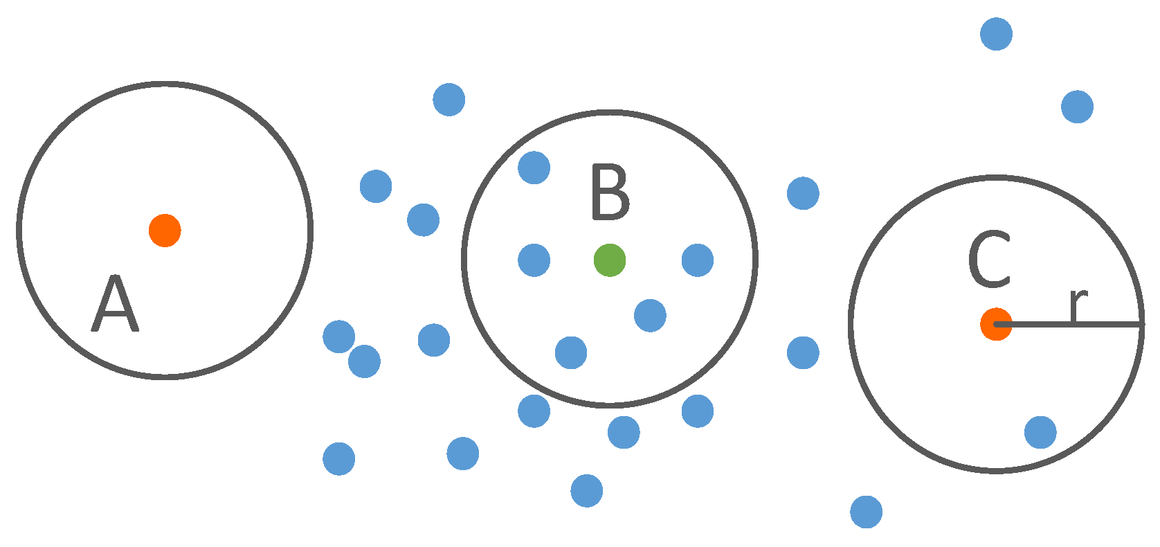
- Remove noise points. Count the number of ALS points within the circular neighborhood of a certain point in 2D space; if the number of points is less than a set threshold, this point is considered a noise point and removed.
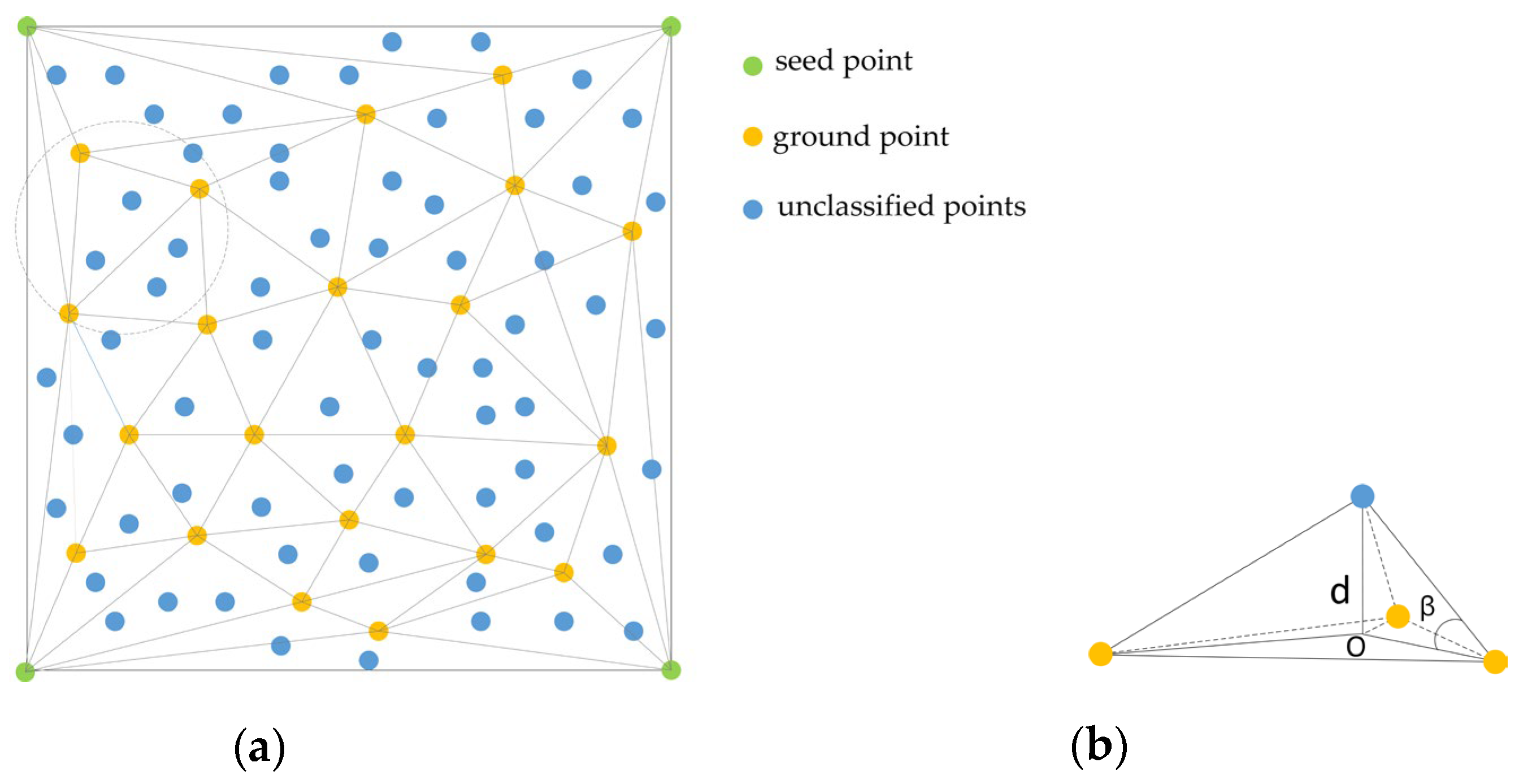
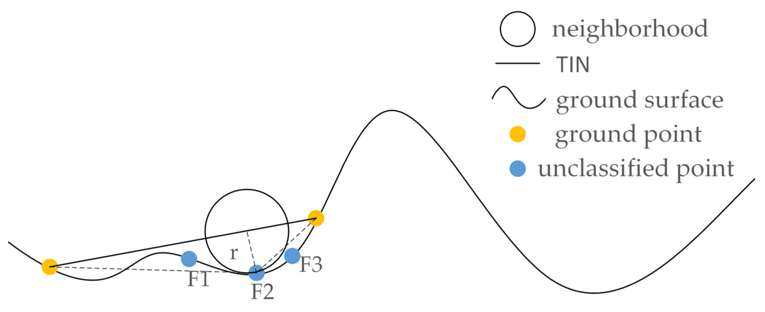
- Select the lowest point within the divided point cloud grid as the initial ground point to construct the densified triangulated irregular network (TIN).
- Optimize the filtered ground point cloud to increase the precision of classification, then the resulting points are normalized to be classified.
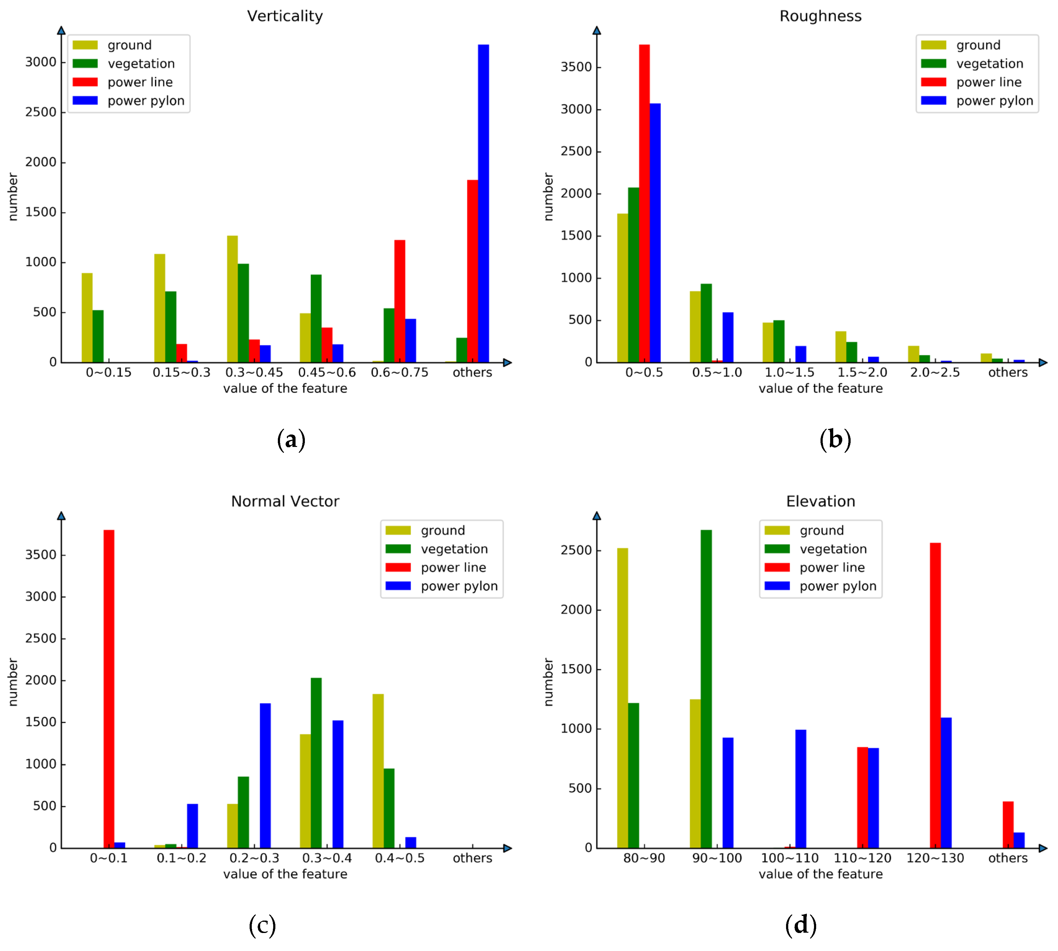
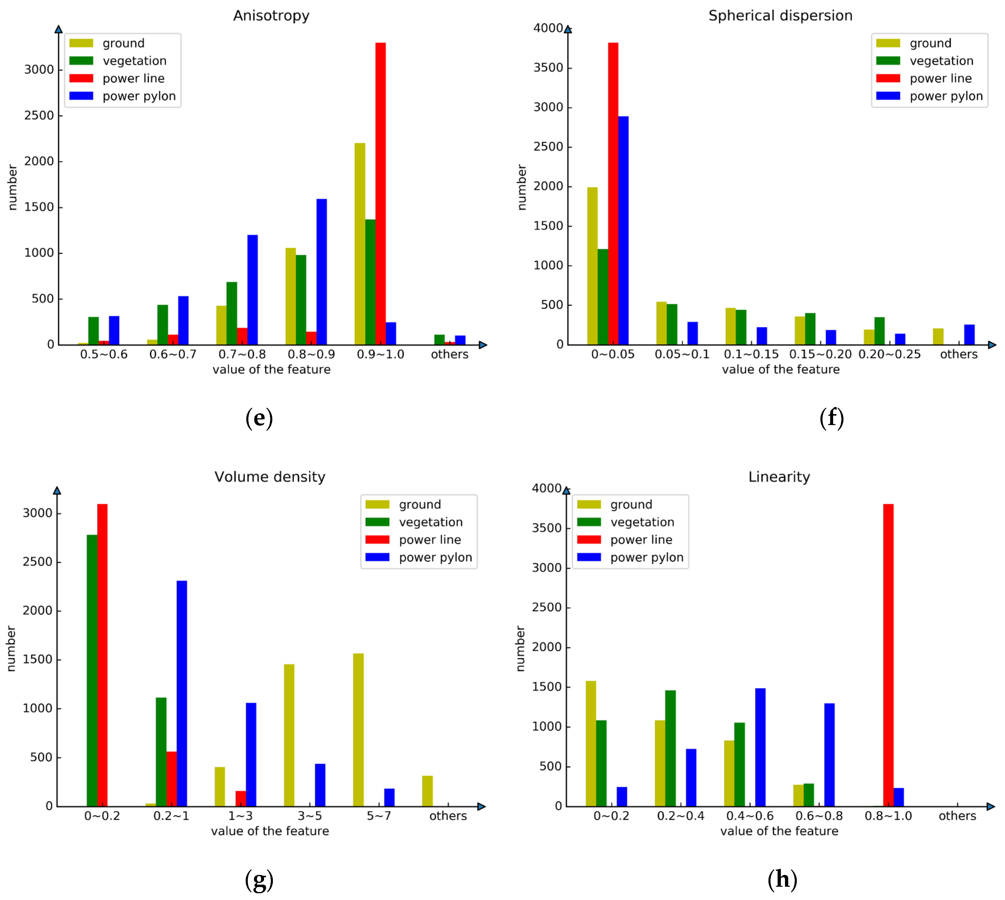
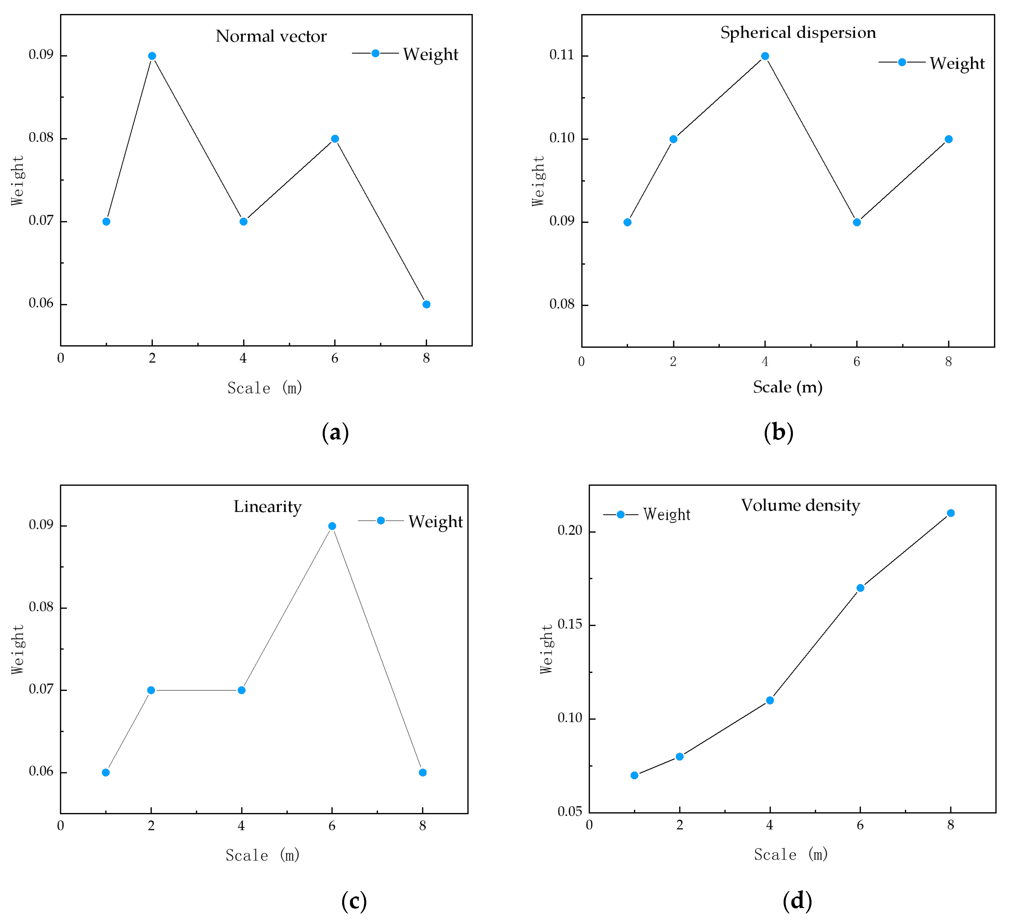
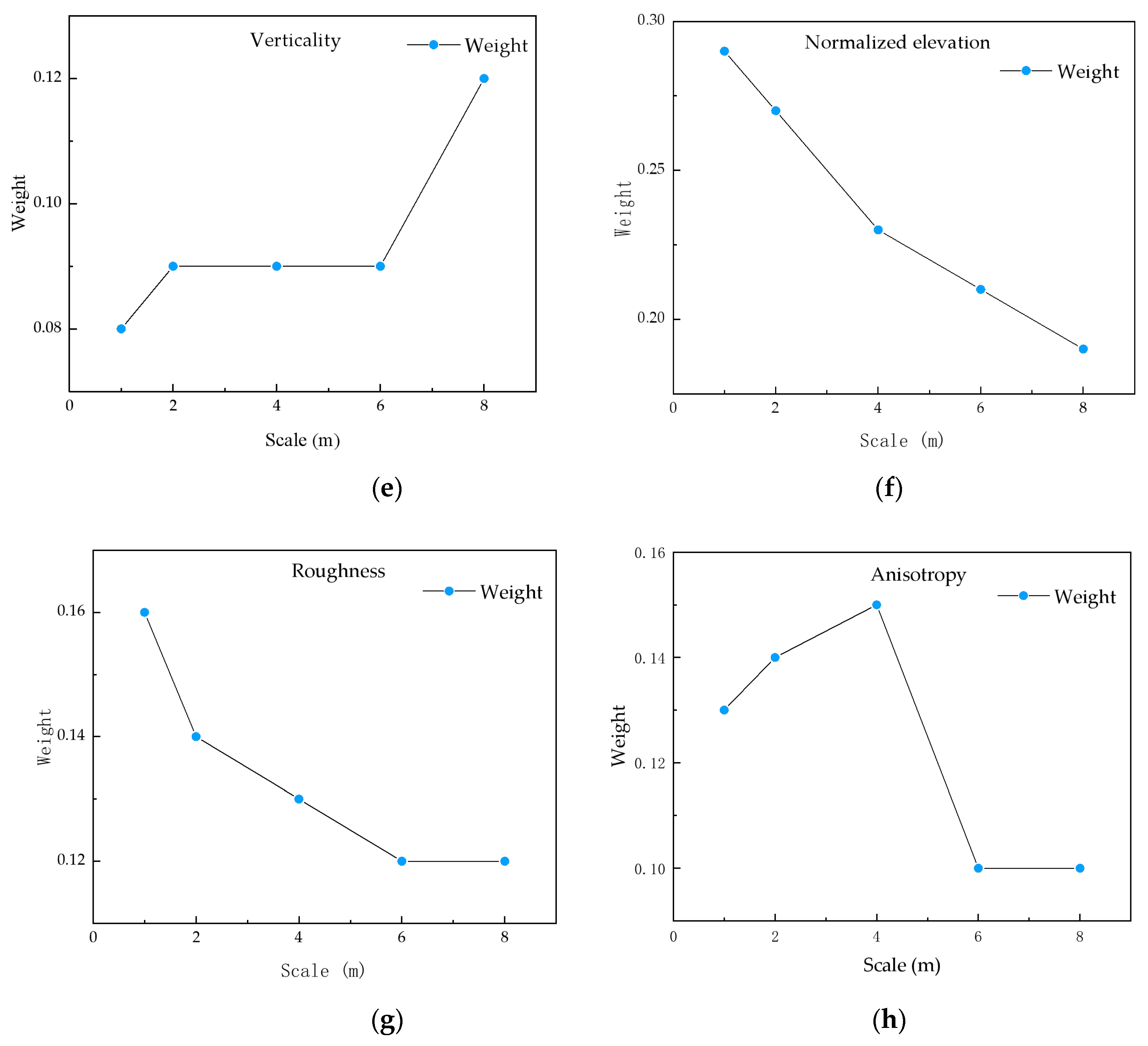
2.2. Multi-Scale Feature Extraction
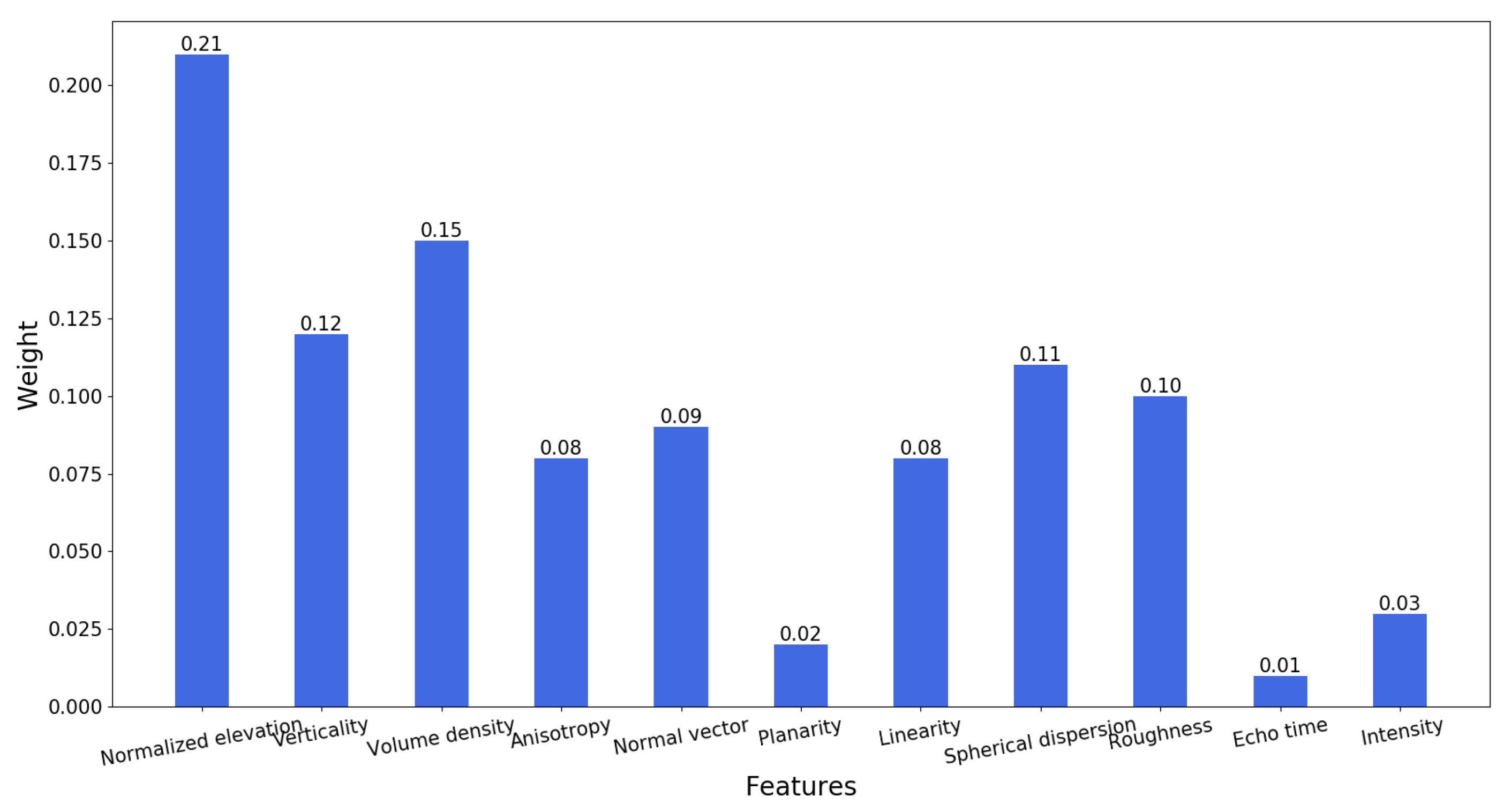
2.3. The Improved Random Forest Algorithm Based on Relief F and SBS
2.3.1. The Related Algorithms
2.3.2. The Improved Random Forest Algorithm
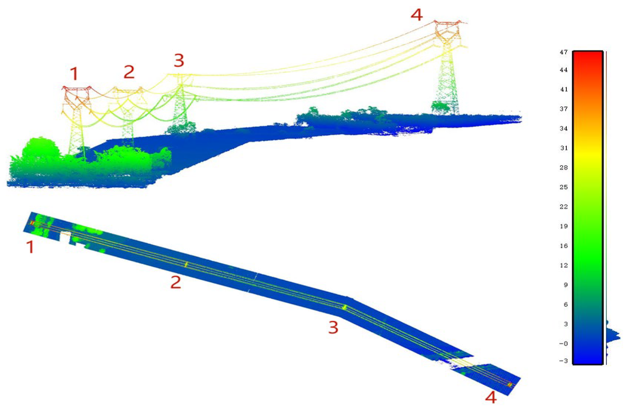
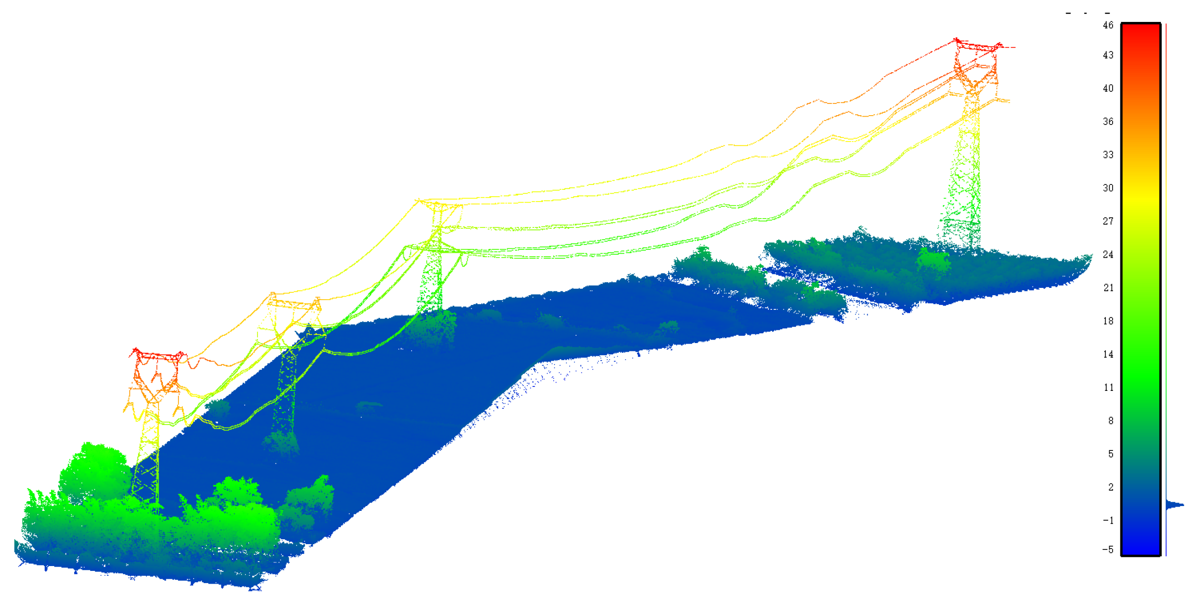
3. Datasets
4. Results and Discussion
4.1. Results of Ground Point Cloud Filtering
4.2. Feature Extraction and Selection
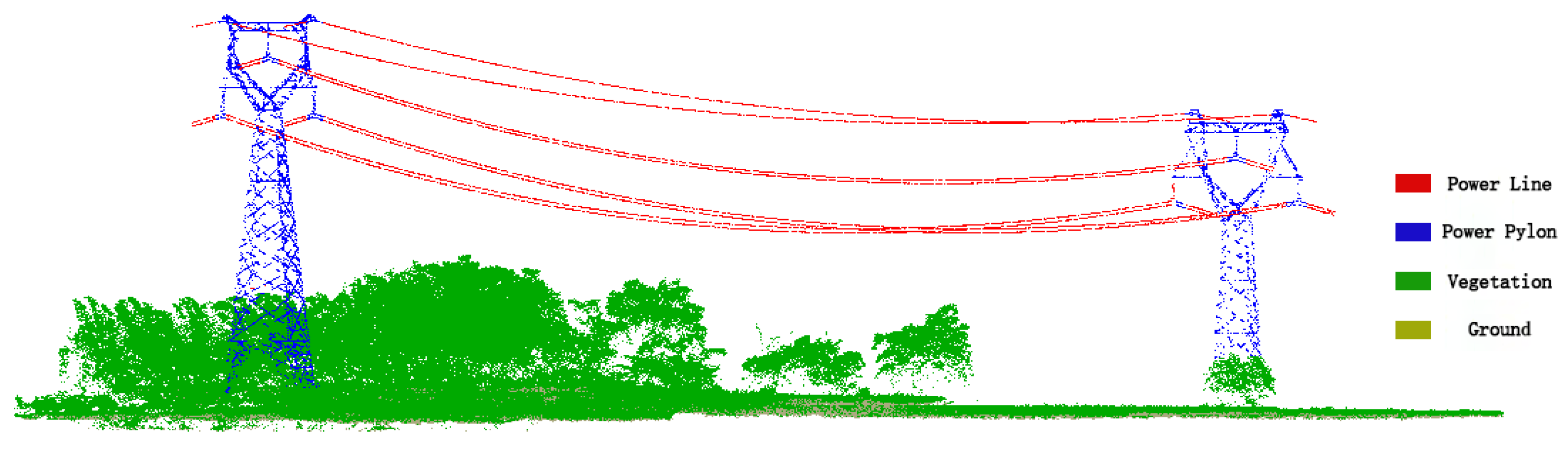
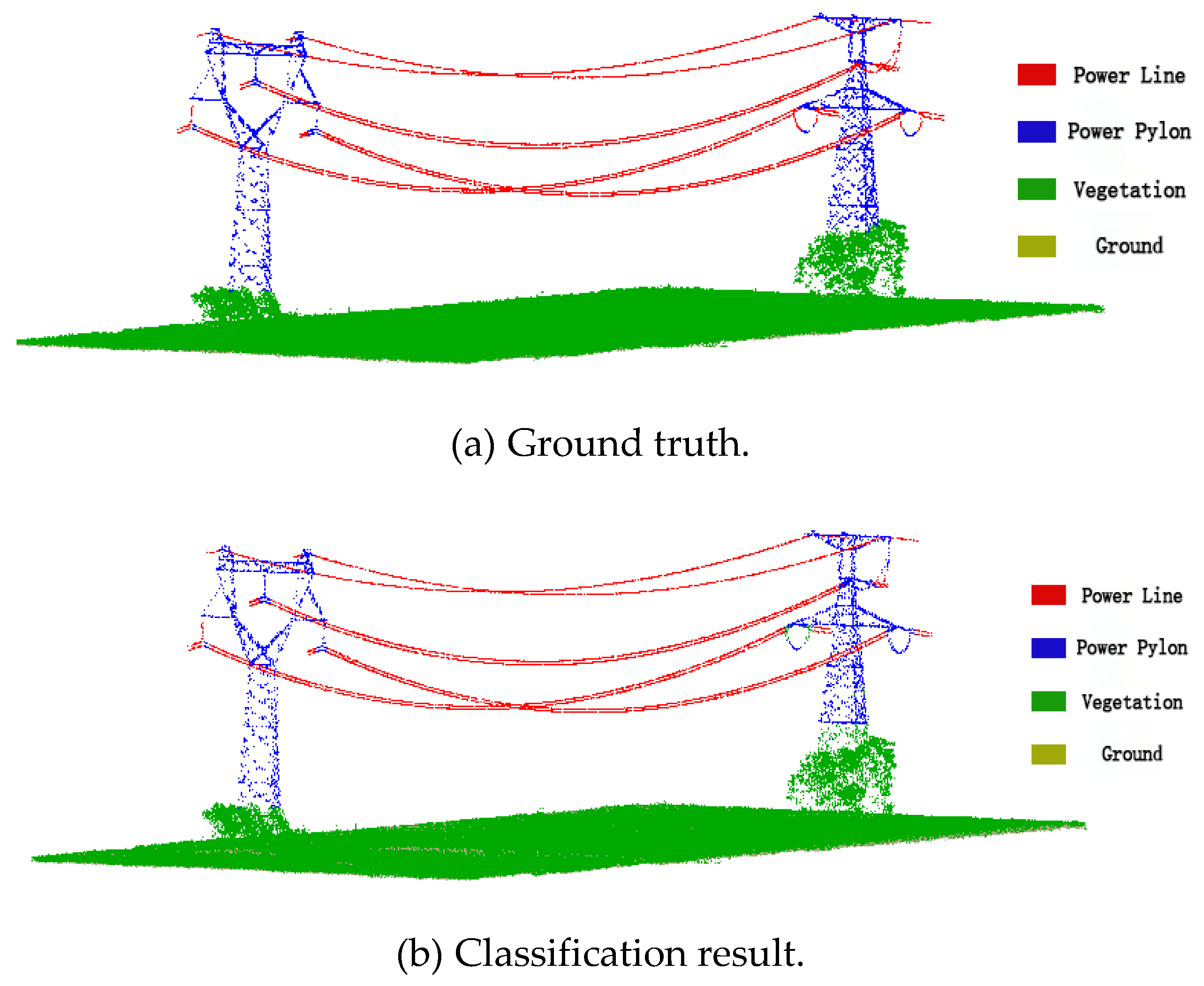
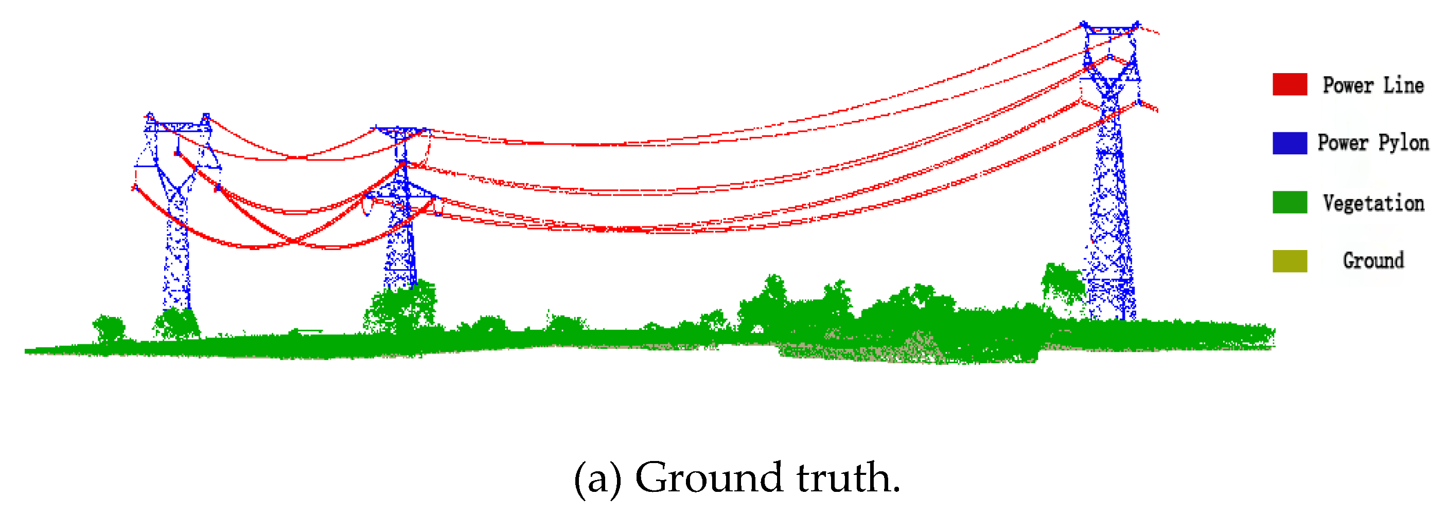
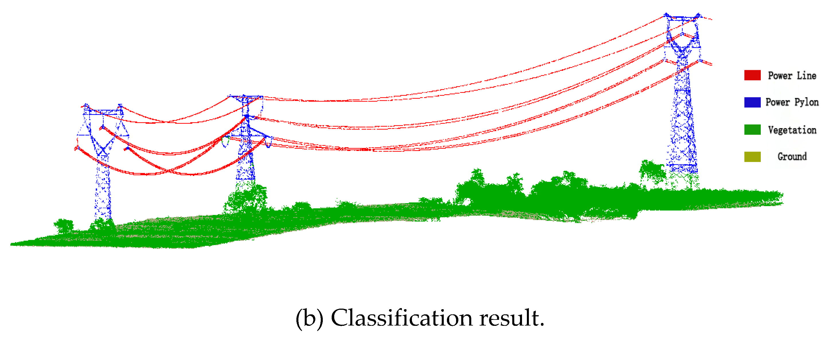
4.3. Classification Results of Transmission Line Point Clouds
4.4. Discussion
5. Conclusions
Author Contributions
Funding
Data Availability Statement
Acknowledgments
Conflicts of Interest
References
- Khalid, H.; Shobole, A. Existing Developments in Adaptive Smart Grid Protection: A Review. Electr. Power Syst. Res. 2021, 191, 106901. [Google Scholar] [CrossRef]
- Judge, M.A.; Khan, A.; Manzoor, A.; Khattak, H.A. Overview of smart grid implementation: Frameworks, impact, performance and challenges. J. Energy Storage 2022, 49, 104056. [Google Scholar] [CrossRef]
- Li, W.; Tang, L.; Wu, H.; Teng, G.; Zhou, M. Development of Mini UAV-borne LiDAR System and It’s Application of Power Line Inspection. Remote Sens. Technol. Appl. 2019, 34, 269–274. [Google Scholar] [CrossRef]
- Kim, H.B.; Sohn, G. Point-based classification of power line corridor scene using random forests. Photogramm. Eng. Remote Sens. 2013, 79, 821–833. [Google Scholar] [CrossRef]
- Guo, B.; Huang, X.; Zhang, F.; Sohn, G. Classification of airborne laser scanning data using JointBoost. ISPRS J. Photogramm. 2015, 100, 71–83. [Google Scholar] [CrossRef]
- Fan, Y.; Zou, R.; Fan, X.; Dong, R.; Xie, M. A Hierarchical Clustering Method to Repair Gaps in Point Clouds of Powerline Corridor for Powerline Extraction. Remote Sens. 2021, 13, 1502. [Google Scholar] [CrossRef]
- Jung, J.; Che, E.; Olsen, M.J.; Shafer, K.C. Automated and efficient powerline extraction from laser scanning data using a voxel-based subsampling with hierarchical approach. ISPRS. J. Photogramm. 2020, 163, 343–361. [Google Scholar] [CrossRef]
- Yang, J.; Kang, Z. Voxel-Based Extraction of Transmission Lines from Airborne LiDAR Point Cloud Data. IEEE J.-Stars 2018, 11, 3892–3904. [Google Scholar] [CrossRef]
- Li, W.; Luo, Z.P.; Xiao, Z.L.; Chen, Y.P.; Wang, C.; Li, J. A GCN-Based Method for Extracting Power Lines and Pylons from Airborne LiDAR Data. IEEE Trans. Geosci. Remote 2022, 60, 1–14. [Google Scholar] [CrossRef]
- Qin, X.; Wu, G.; Ye, X.; Huang, L.; Lei, J. A Novel Method to Reconstruct Overhead High-Voltage Power Lines Using Cable Inspection Robot LiDAR Data. Remote Sens. 2017, 9, 753. [Google Scholar] [CrossRef]
- Pastucha, E.; Puniach, E.; Ścisłowicz, A.; Ćwiąkała, P.; Niewiem, W.; Wiącek, P. 3D Reconstruction of Power Lines Using UAV Images to Monitor Corridor Clearance. Remote Sens. 2020, 12, 3698. [Google Scholar] [CrossRef]
- Guo, B.; Huang, X.; Li, Q.; Zhang, F.; Zhu, J.; Wang, C. A Stochastic Geometry Method for Pylon Reconstruction from Airborne LiDAR Data. Remote Sens. 2016, 8, 243. [Google Scholar] [CrossRef] [Green Version]
- Chen, S.; Wang, C.; Dai, H.; Zhang, H.; Pan, F.; Xi, X.; Yan, Y.; Wang, P.; Yang, X.; Zhu, X.; et al. Power Pylon Reconstruction Based on Abstract Template Structures Using Airborne LiDAR Data. Remote Sens. 2019, 11, 1579. [Google Scholar] [CrossRef] [Green Version]
- Rau, J.-Y.; Jhan, J.-P.; Hsu, Y.C. Analysis of Oblique Aerial Images for Land Cover and Point Cloud Classification in an Urban Environment. IEEE Trans. Geosci. Remote 2015, 53, 1304–1319. [Google Scholar] [CrossRef]
- Pan, S.; Guan, H.; Yu, Y.; Li, J.; Peng, D. A Comparative Land-Cover Classification Feature Study of Learning Algorithms: DBM, PCA and RF Using Multispectral LiDAR Data. IEEE J.-Stars 2019, 12, 1314–1326. [Google Scholar] [CrossRef]
- Liu, Y.; Aleksandrov, M.; Zlatanova, S.; Zhang, J.; Mo, F.; Chen, X. Classification of Power Facility Point Clouds from Unmanned Aerial Vehicles Based on Adaboost and Topological Constraints. Sensors 2019, 19, 4717. [Google Scholar] [CrossRef] [Green Version]
- Ni, H.; Lin, X.; Zhang, J. Classification of ALS Point Cloud with Improved Point Cloud Segmentation and Random Forests. Remote Sens. 2017, 9, 288. [Google Scholar] [CrossRef] [Green Version]
- Zhang, J.; Lin, X.; Ning, X. SVM-Based Classification of Segmented Airborne LiDAR Point Clouds in Urban Areas. Remote Sens. 2013, 5, 3749–3775. [Google Scholar] [CrossRef] [Green Version]
- Moorthy, S.M.K.; Calders, K.; Vicari, M.B.; Verbeeck, H. Improved supervised learning-based approach for leaf and wood classification from LiDAR point clouds of forests. IEEE. Trans. Geosci. Remote 2020, 58, 3057–3070. [Google Scholar] [CrossRef] [Green Version]
- Yu, Y.; Li, J.; Guan, H.; Jia, F.; Wang, C. Learning Hierarchical Features for Automated Extraction of Road Markings From 3-D Mobile LiDAR Point Clouds. IEEE J-Stars 2015, 8, 709–726. [Google Scholar] [CrossRef]
- Zhang, Z.; Zhang, L.; Tong, X.; Mathiopoulos, P.T.; Guo, B.; Huang, X.; Wang, Z.; Wang, Y. A Multilevel Point-Cluster-Based Discriminative Feature for ALS Point Cloud Classification. IEEE Trans. Geosci. Remote 2016, 54, 3309–3321. [Google Scholar] [CrossRef]
- Zheng, L.; Li, Z. Virtual Namesake Point Multi-Source Point Cloud Data Fusion Based on FPFH Feature Difference. Sensors 2021, 21, 5441. [Google Scholar] [CrossRef] [PubMed]
- Mallet, C.; Bretar, F.; Roux, M.; Soergel, U.; Heipke, C. Relevance assessment of full-waveform lidar data for urban area classification. ISPRS J. Photogramm. 2011, 66, S71–S84. [Google Scholar] [CrossRef]
- Wang, Z.; Zhang, L.; Fang, T.; Mathiopoulos, P.T.; Tong, X.; Qu, H.; Xiao, Z.; Li, F.; Chen, D. A Multiscale and Hierarchical Feature Extraction Method for Terrestrial Laser Scanning Point Cloud Classification. IEEE Trans. Geosci. Remote 2015, 53, 2409–2425. [Google Scholar] [CrossRef]
- Weinmann, M.; Jutzi, B.; Hinz, S.; Mallet, C. Semantic point cloud interpretation based on optimal neighborhoods, relevant features and efficient classifiers. ISPRS J. Photogramm. 2015, 105, 286–304. [Google Scholar] [CrossRef]
- Wang, Y.; Chen, Q.; Liu, L.; Zheng, D.; Li, C.; Li, K. Supervised Classification of Power Lines from Airborne LiDAR Data in Urban Areas. Remote Sens. 2017, 9, 771. [Google Scholar] [CrossRef] [Green Version]
- Mukhopadhyay, P.; Chaudhuri, B.B. A survey of Hough Transform. Pattern Recogn. 2015, 48, 993–1010. [Google Scholar] [CrossRef]
- Wang, P.H.; Xi, X.H.; Wang, C.; Xia, S.B. Study on power line fast extraction based on airborne LiDAR data. Sci. Surv. Mapp. 2017, 42, 6. [Google Scholar] [CrossRef]
- Chum, O.; Matas, J. Optimal Randomized RANSAC. IEEE Trans. Pattern Anal. Mach. Intell. 2008, 30, 1472–1482. [Google Scholar] [CrossRef] [Green Version]
- Reyes, O.; Morell, C.; Ventura, S. Scalable extensions of the ReliefF algorithm for weighting and selecting features on the multi-label learning context. Neurocomputing 2015, 161, 168–182. [Google Scholar] [CrossRef]
- Cotter, S.F.; Kreutz-Delgado, K.; Rao, B.D. Backward sequential elimination for sparse vector subset selection. Signal Process. 2001, 81, 1849–1864. [Google Scholar] [CrossRef]
- Zhao, X.; Guo, Q.; Su, Y.; Xue, B. Improved progressive TIN densification filtering algorithm for airborne LiDAR data in forested areas. ISPRS J. Photogramm. 2016, 117, 79–91. [Google Scholar] [CrossRef] [Green Version]
- Wang, Z. Recognition of occluded objects by slope difference distribution features. Appl. Soft Comput. 2022, 120, 108622. [Google Scholar] [CrossRef]
- Chen, Q.; Dam, T.V.; Sneeuw, N.; Collilieux, X.; Weigelt, M.; Rebischung, P. Singular spectrum analysis for modeling seasonal signals from GPS time series. J. Geodyn. 2013, 72, 25–35. [Google Scholar] [CrossRef]
- Mirzaei, K.; Arashpour, M.; Asadi, E.; Masoumi, H.; Bai, Y.; Behnood, A. 3D point cloud data processing with machine learning for construction and infrastructure applications: A comprehensive review. Adv. Eng. Inform. 2022, 51, 101501. [Google Scholar] [CrossRef]
- Zeng, Q.; Mao, J.; Li, X.; Liu, X. Bulding roof boundary extraction from LiDAR point cloud. Geomat. Inf. Sci. Wuhan Univ. 2009, 34, 383–386. [Google Scholar]
- Guo, Y.; Bennamoun, M.; Sohel, F.; Lu, M.; Wan, J. 3D Object Recognition in Cluttered Scenes with Local Surface Features: A Survey. IEEE Trans. Pattern Anal. Mach. Intell. 2014, 36, 2270–2287. [Google Scholar] [CrossRef]
- Atik, M.E.; Duran, Z.; Seker, D.Z. Machine Learning-Based Supervised Classification of Point Clouds Using Multiscale Geometric Features. ISPRS Int. J. Geo-Inf. 2021, 10, 187. [Google Scholar] [CrossRef]
- Mills, G.; Fotopoulos, G. Rock Surface Classification in a Mine Drift Using Multiscale Geometric Features. IEEE Trans. Geosci. Remote Sens. 2015, 12, 1322–1326. [Google Scholar] [CrossRef]
- Ma, Z.; Pang, Y.; Li, Z.; Lu, H.; Liu, L.; Chen, B. Fine classification of near-ground point cloud based on terrestrial laser scanning and detection of forest fallen wood. J. Remote Sens 2019, 23, 743–755. [Google Scholar] [CrossRef]
- Xiong, Y.; Gao, R.; Xu, Z. Random forest method for dimension reduction and point cloud classification based on airborne LiDAR. Acta Geod. Et Cartogr. Sin. 2018, 47, 508–518. [Google Scholar] [CrossRef]
- Chen, X.; Chen, Z.; Liu, G.; Chen, K.; Wang, L.; Xiang, W.; Zhang, R. Railway Overhead Contact System Point Cloud Classification. Sensors 2021, 21, 4961. [Google Scholar] [CrossRef] [PubMed]
- Yan, Y.; Yan, H.; Guo, J.; Dai, H. Classification and Segmentation of Mining Area Objects in Large-Scale Spares Lidar Point Cloud Using a Novel Rotated Density Network. ISPRS Int. J. Geo-Inf. 2020, 9, 182. [Google Scholar] [CrossRef] [Green Version]
- Mills, G.; Fotopoulos, G. On the estimation of geological surface roughness from terrestrial laser scanner point clouds. Geosphere 2013, 9, 1410–1416. [Google Scholar] [CrossRef]
- Breiman, L. Random forests. Mach. Learn. 2001, 45, 5–32. [Google Scholar] [CrossRef] [Green Version]
- Shi, S.; Bi, S.; Gong, W.; Chen, B.; Chen, B.; Tang, X.; Qu, F.; Song, S. Land Cover Classification with Multispectral LiDAR Based on Multi-Scale Spatial and Spectral Feature Selection. Remote Sens. 2021, 13, 4118. [Google Scholar] [CrossRef]


| Category | Point Cloud Features | Scales |
|---|---|---|
| ground | Linearity () Planarity () Anisotropy () Spherical dispersion () Normal vector () Volume density () Verticality () Roughness () | 1 m 2 m 4 m 6 m 8 m |
| building | ||
| vegetation | ||
| power line | ||
| power pylon |
| Dataset | Area (m2) | Density (pt/m2) | Number of Points |
|---|---|---|---|
| Training set A | 331 × 52 | 79 | 1,362,684 |
| Testing set B | 342 × 52 | 65 | 1,158,634 |
| Testing set C | 721 × 52 | 64 | 2,411,158 |
| Overall Accuracy: 98.73% | |||||
|---|---|---|---|---|---|
| Category | Ground | Vegetation | Power Line | Power Pylon | Recall/% |
| ground | 30,703 | 8086 | 0 | 0 | 80.18 |
| vegetation | 6015 | 1,101,805 | 0 | 282 | 99.43 |
| power line | 0 | 0 | 7220 | 279 | 96.27 |
| power pylon | 0 | 228 | 265 | 7851 | 94.09 |
| Precision/% | 83.61 | 99.25 | 96.45 | 93.33 | |
| Overall accuracy: 99.1% | |||||
|---|---|---|---|---|---|
| Category | Ground | Vegetation | Power Line | Power Pylon | Recall/% |
| ground | 57,914 | 10,304 | 0 | 0 | 84.89 |
| vegetation | 9811 | 2,302,050 | 50 | 40 | 99.57 |
| power line | 0 | 15 | 15,950 | 754 | 95.4 |
| power pylon | 0 | 328 | 619 | 13,323 | 93.36 |
| Precision/% | 85.51 | 99.53 | 95.97 | 94.38 | |
Disclaimer/Publisher’s Note: The statements, opinions and data contained in all publications are solely those of the individual author(s) and contributor(s) and not of MDPI and/or the editor(s). MDPI and/or the editor(s) disclaim responsibility for any injury to people or property resulting from any ideas, methods, instructions or products referred to in the content. |
© 2023 by the authors. Licensee MDPI, Basel, Switzerland. This article is an open access article distributed under the terms and conditions of the Creative Commons Attribution (CC BY) license (https://creativecommons.org/licenses/by/4.0/).
Share and Cite
Tang, Q.; Zhang, L.; Lan, G.; Shi, X.; Duanmu, X.; Chen, K. A Classification Method of Point Clouds of Transmission Line Corridor Based on Improved Random Forest and Multi-Scale Features. Sensors 2023, 23, 1320. https://doi.org/10.3390/s23031320
Tang Q, Zhang L, Lan G, Shi X, Duanmu X, Chen K. A Classification Method of Point Clouds of Transmission Line Corridor Based on Improved Random Forest and Multi-Scale Features. Sensors. 2023; 23(3):1320. https://doi.org/10.3390/s23031320
Chicago/Turabian StyleTang, Qingyun, Letan Zhang, Guiwen Lan, Xiaoyong Shi, Xinghui Duanmu, and Kan Chen. 2023. "A Classification Method of Point Clouds of Transmission Line Corridor Based on Improved Random Forest and Multi-Scale Features" Sensors 23, no. 3: 1320. https://doi.org/10.3390/s23031320