
Performance Analysis of Localization Algorithms for Inspections in 2D and 3D Unstructured Environments Using 3D Laser Sensors and UAVs

 , , , , , and
Abstract
:1. Introduction
2. Related Work
3. Methodology
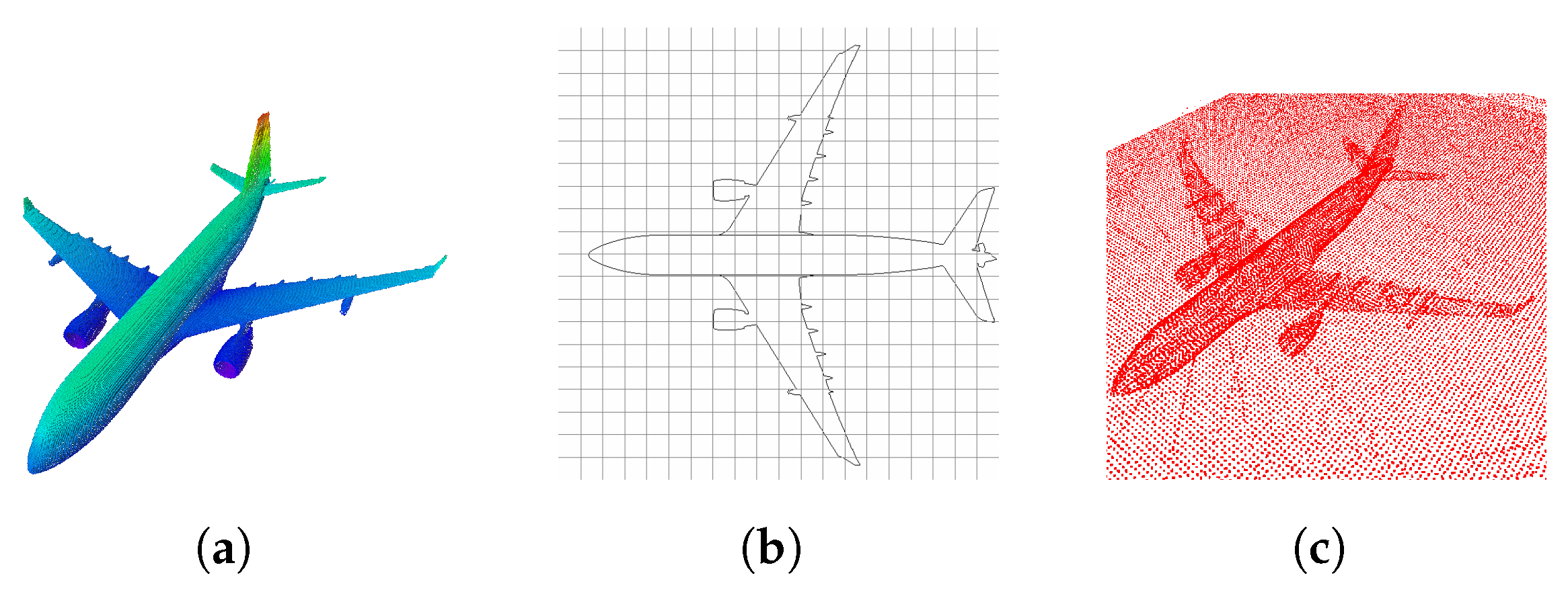
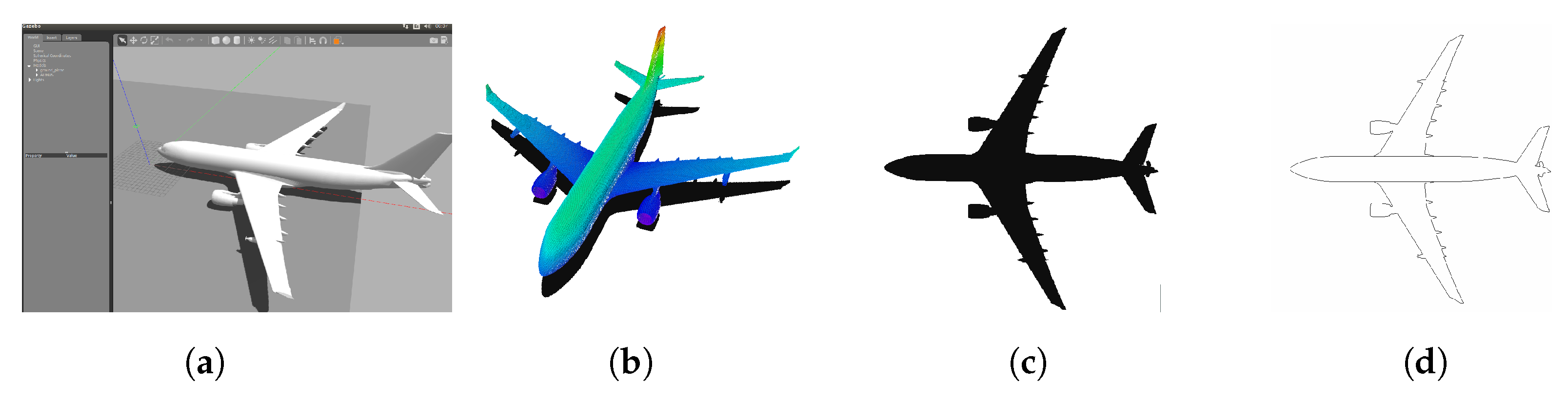
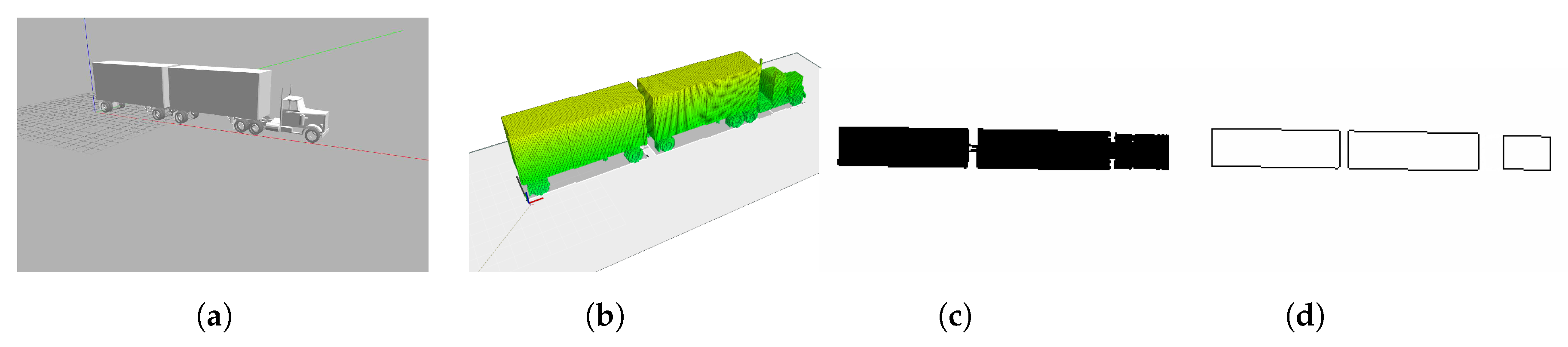
3.1. Maps
3.2. 2D Localization
- X, current set of particles.
- , the previous set of particles.
- , last motion and odometry measurements.
- , last laser rangefinder measurements.
- m, max number of particles.
- Motion kinematics: e.g., differential or omnidirectional.
- Uncertainty of the robot odometry, which determines the error in translation or rotation .
- Observation model: e.g., beam model or probability field model.
- Measurements errors: e.g., measurement noise , unexpected objects , object detection failures , unexplained random noise .
- Number of random particles, defined by the probabilities of long-term and short-term measurements.
3.3. 3D Localization
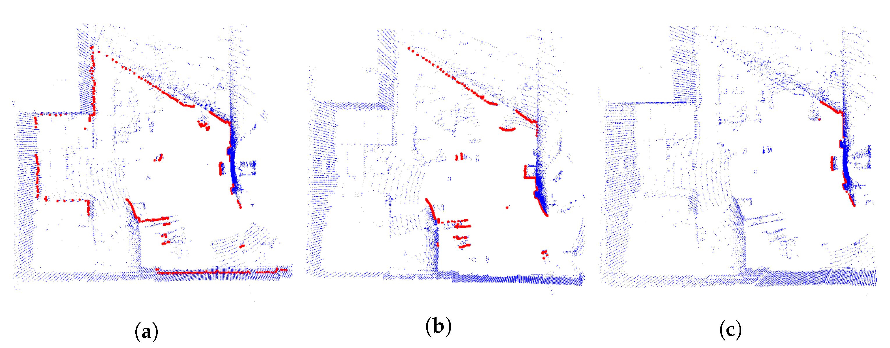
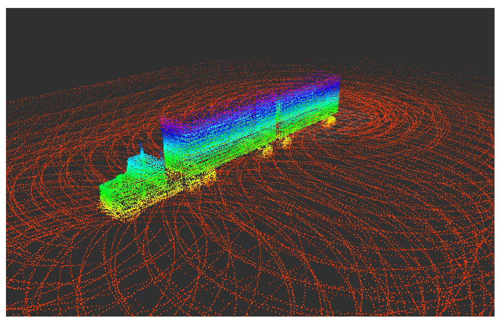
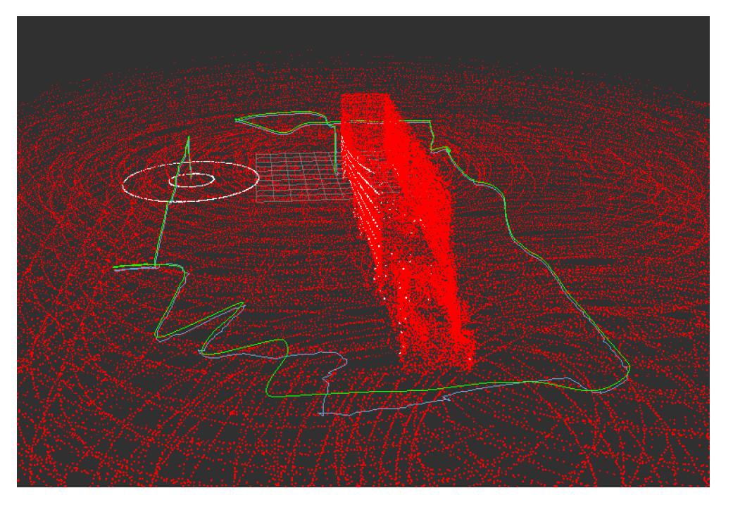
- Subsampling: Reduction of the number of points in the sample using Voxel grid filter and Pass-through Filter techniques [49] to optimize processing time.
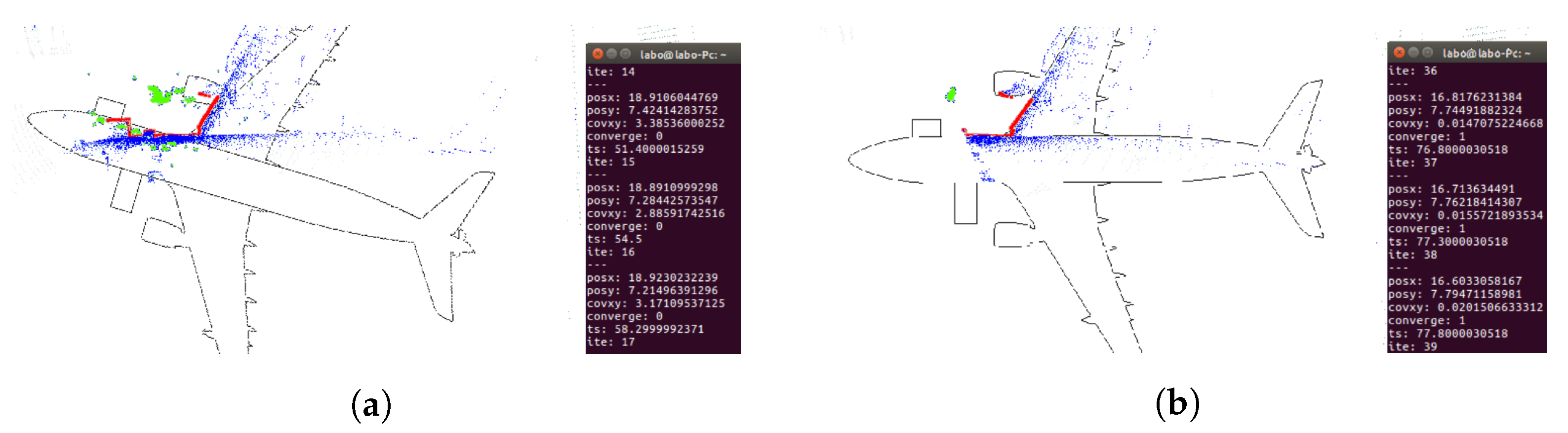
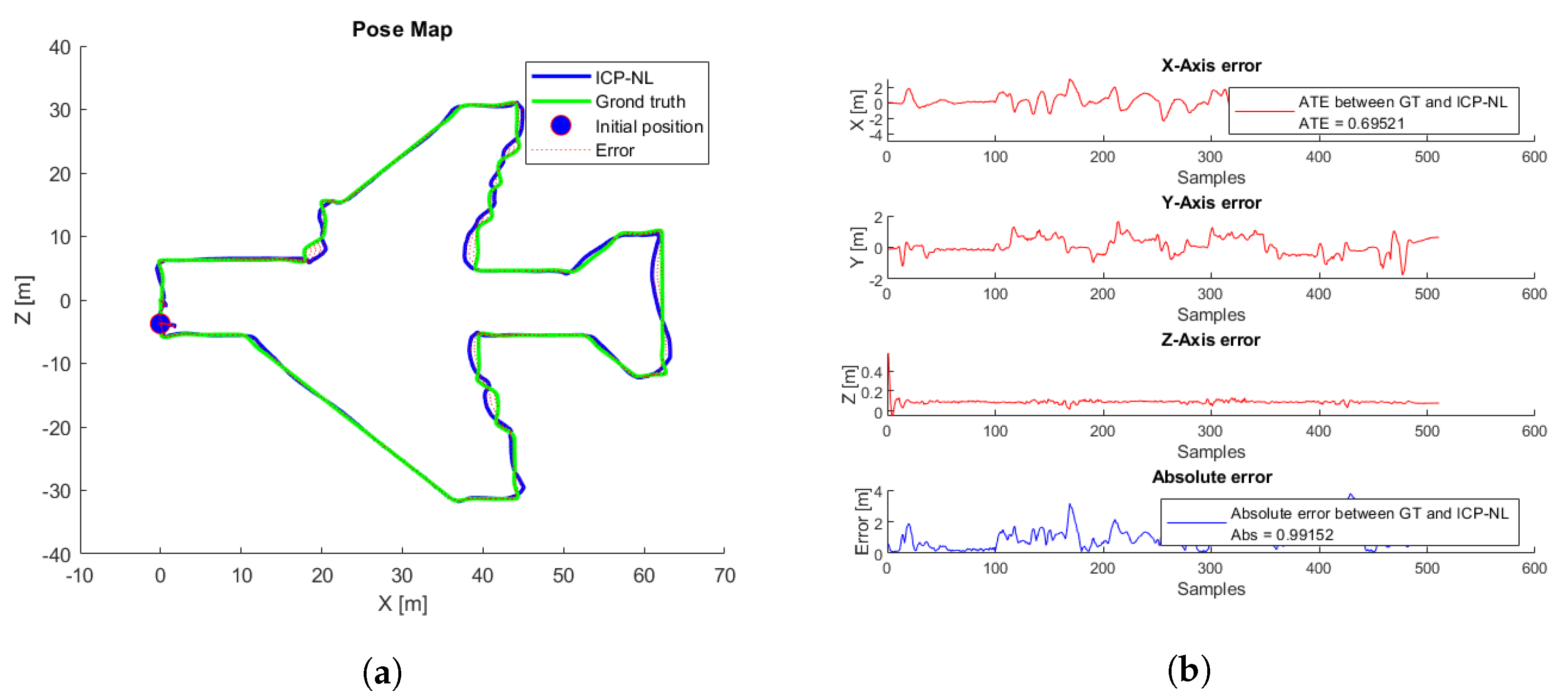
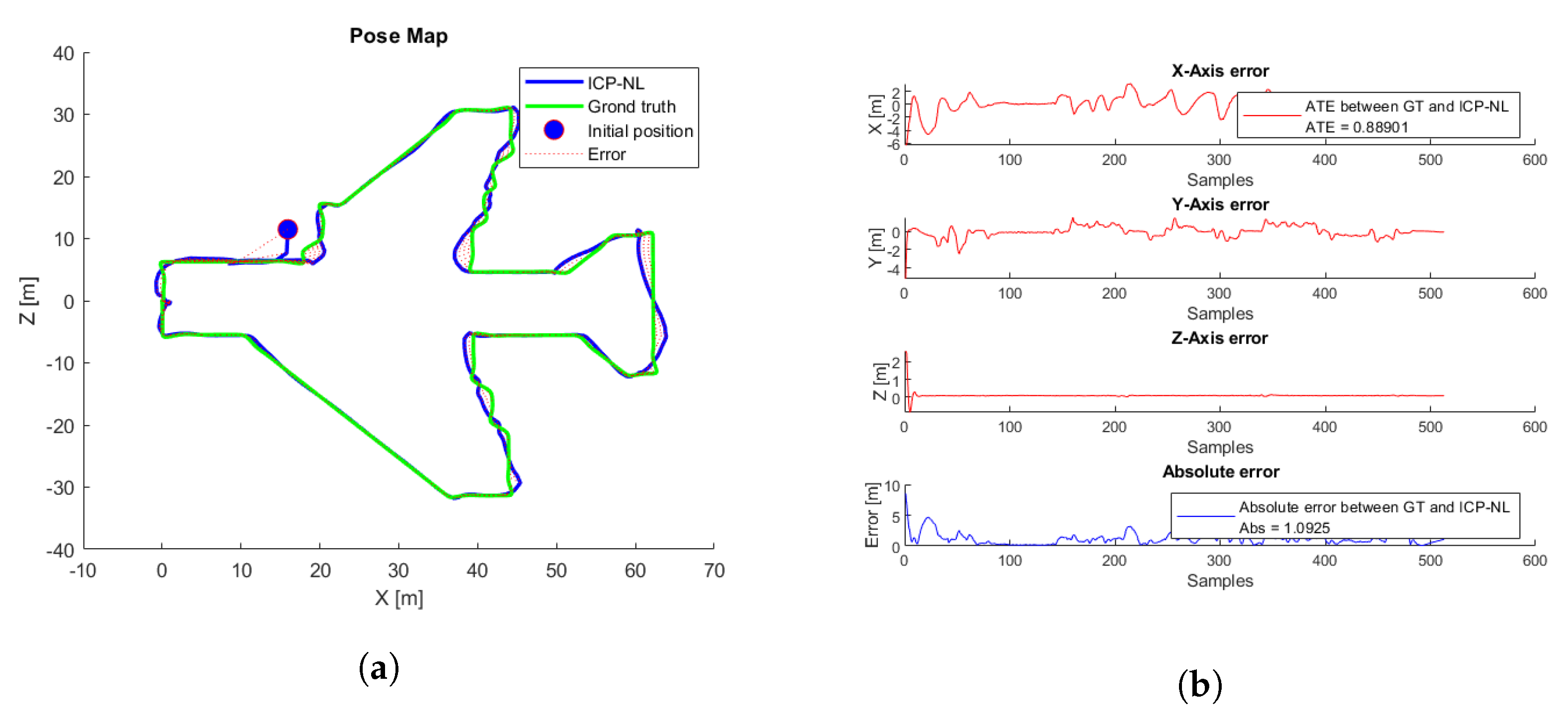
- Pose estimation with nonlinear ICP: Based on the ICP technique presented in [50]. It takes as inputs a source and a target point cloud matched under the nearest-neighbor criterion. Singular Value Decomposition (SVD) is applied to obtain an estimate of the transformation matrix that aligns them. This process is repeated until a termination criterion is met, removing outliers and redefining the correspondences.
- Unscented Kalman Filter-based localization: This is an improvement of EKF for application to highly nonlinear systems. This approach uses the unscented transform to take a set of samples called sigma points, which are propagated by nonlinear functions and used to calculate the mean and variance. Unlike EKF, UKF eliminates the need for a Jacobian, facilitating calculations on complex functions.
| Algorithm 1: Localization 3D (, , , , ) |
 |
4. Results
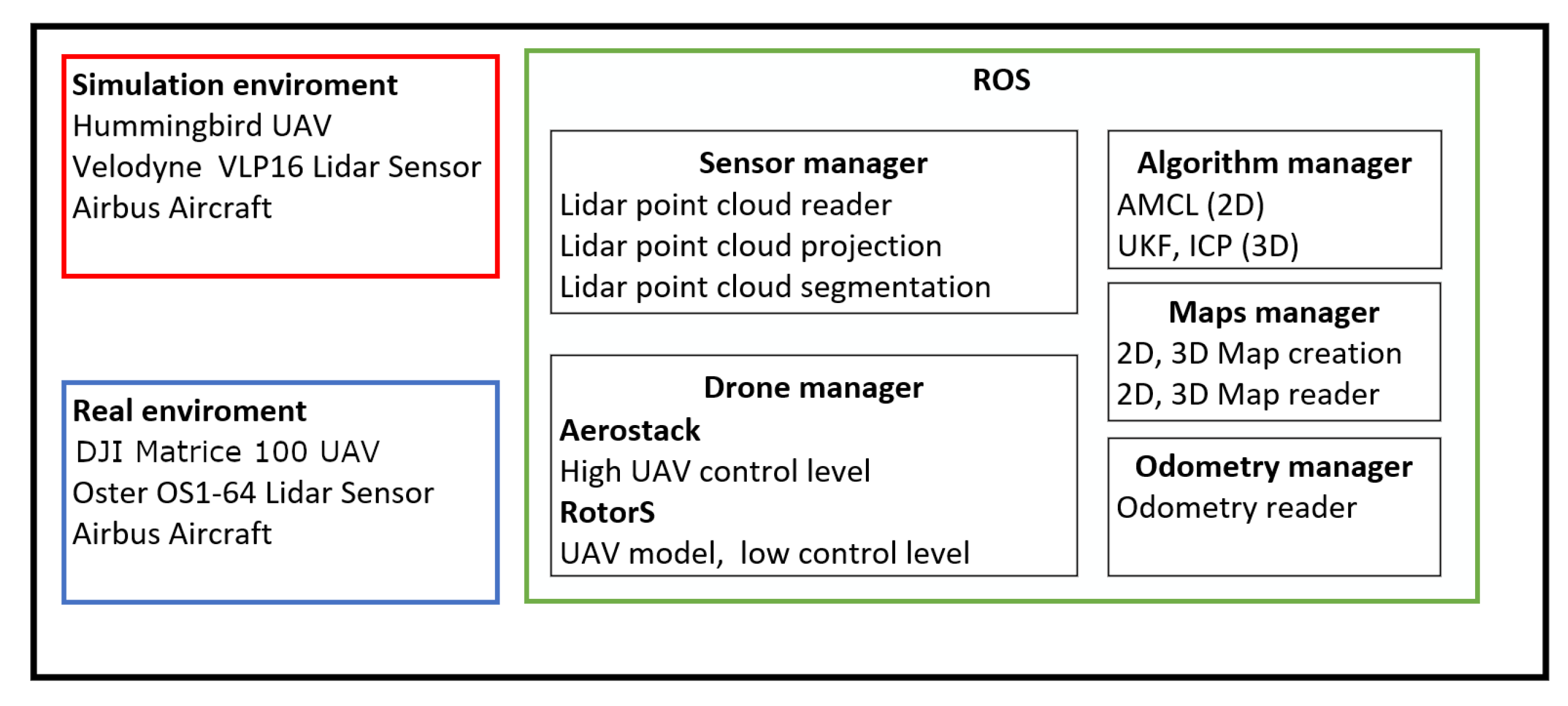
4.1. Software
4.2. Hardware
- Personal Computer (PC) Intel core i7 2.70 GHz, 4 Gb RAM.
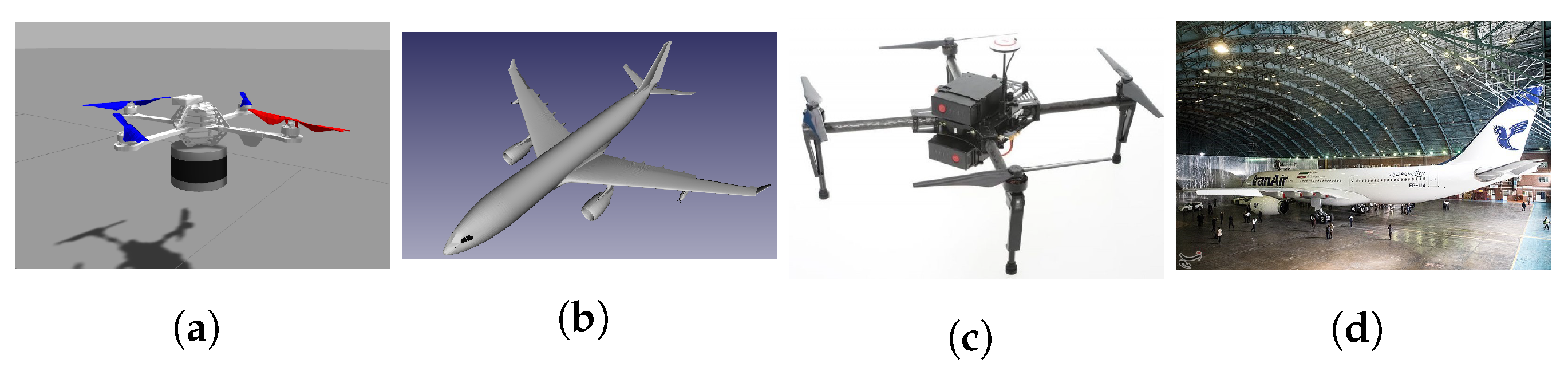
- Hummingbird UAV provided by Rotors (Figure 6a).
- Odometry measurements from a configurable odometry sensor (see Appendix A for configuration details).
- Velodyne VLP16 3D laser sensor [55] provides a point cloud with 300,000 points per second and ±3 cm accuracy, 100 m range, 360° horizontal and 30° vertical field of view (see Appendix B for setting other parameters). Due to computational limitations in the simulation, we worked with 5120 points per second.
- Manifold Intel i7 1.8 Ghz, 2 GB RAM.
- DJI Matrice 100 UAV (Figure 6c).
- Odometry measurements were provided by a sensor fusion algorithm [56] that merges the onboard DJI sensors: Altimeter, Velocity and IMU, plus the 3D Light Detection and Ranging (LIDAR) IMU.
- 3D LIDAR Ouster OS1-64, providing a point cloud with 327,680 points per second and ±1 cm accuracy 100 m range, 0.3 cm resolution, 360° horizontal and 45° vertical field of view.
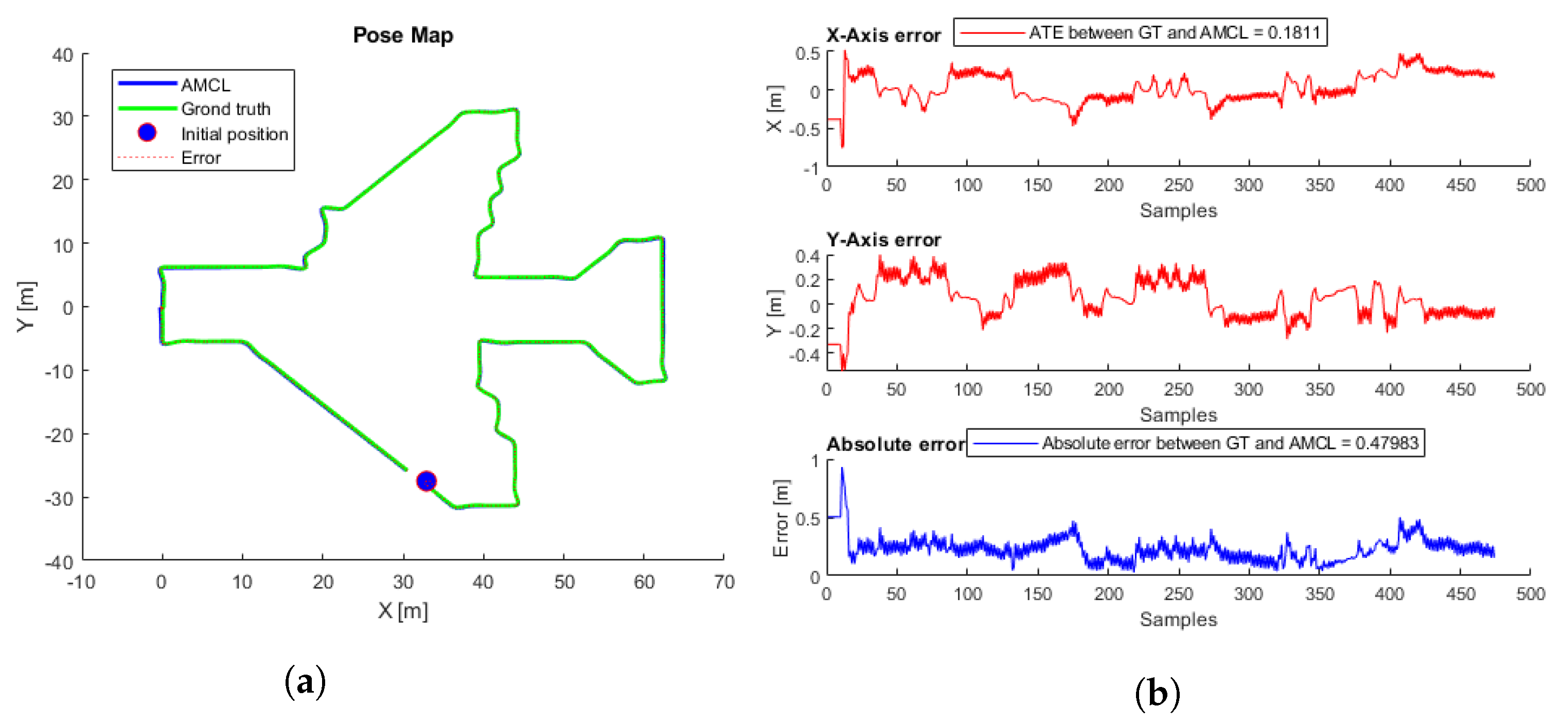
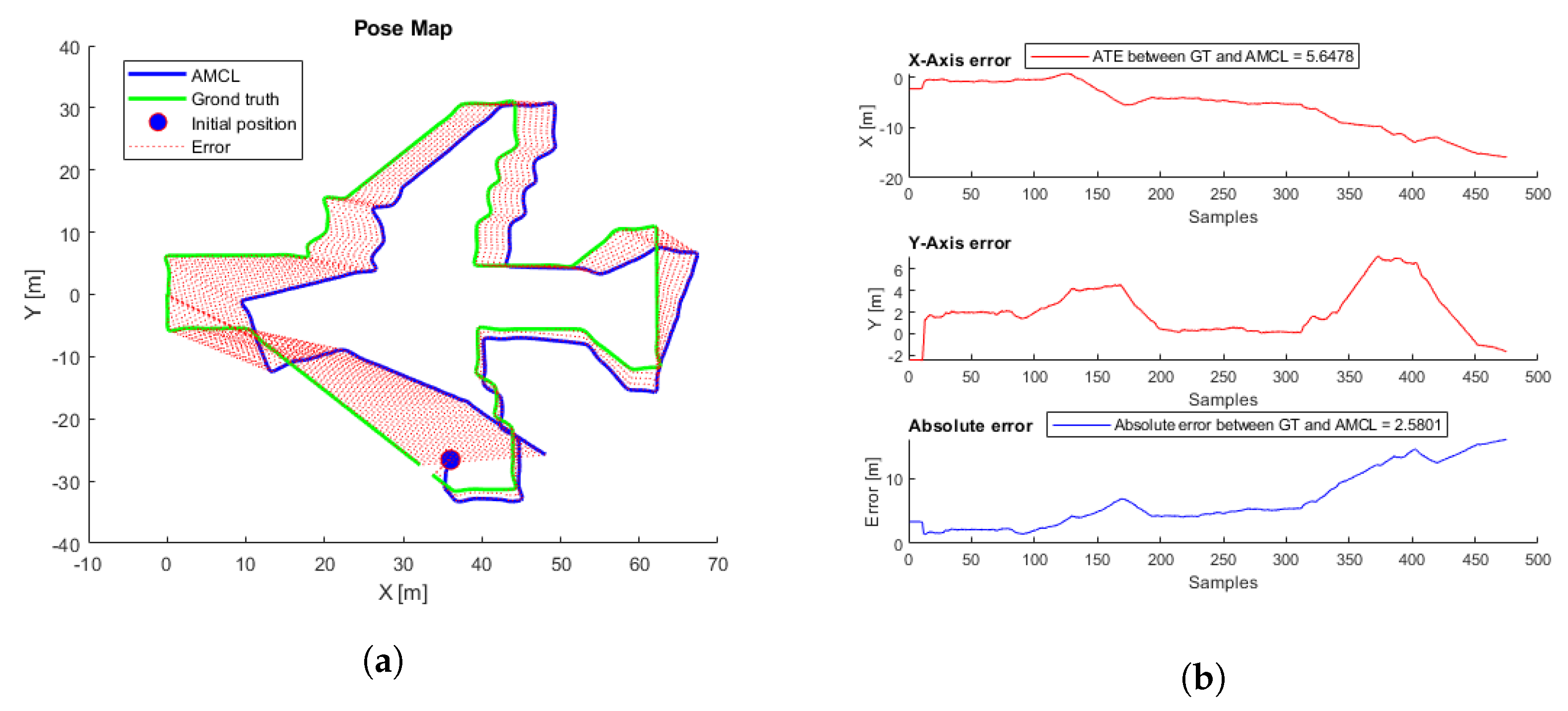
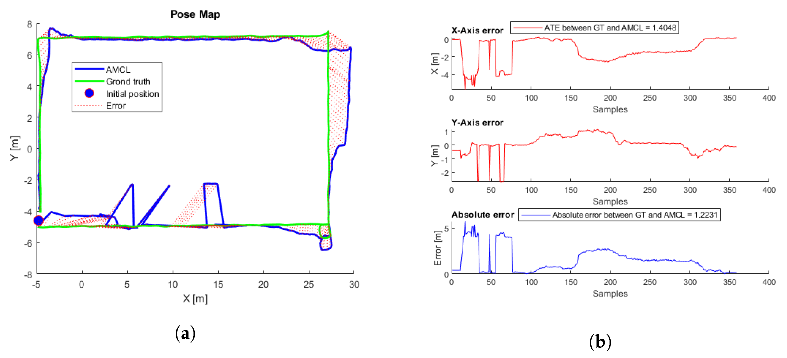
4.3. Error Metric
- , is the magnitude of the Euclidean distance along the horizontal plane between the estimated and ground-truth poses at frame i.
- n, number of frames.
4.4. 2D Localization
4.4.1. Simulation Tests
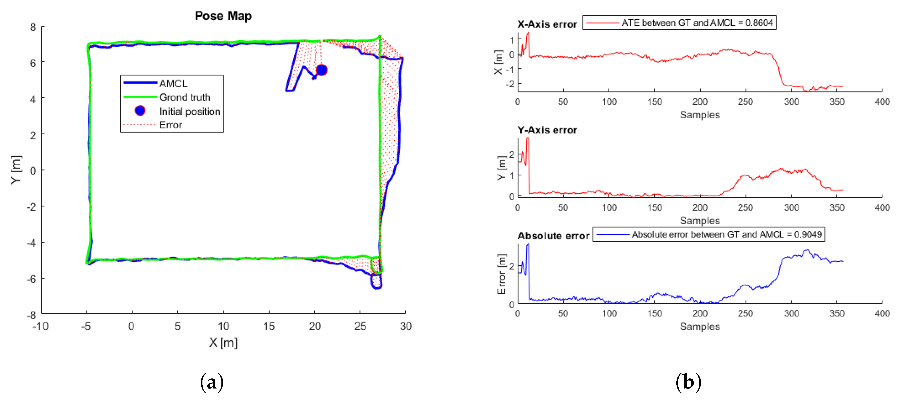
4.4.2. Real Tests
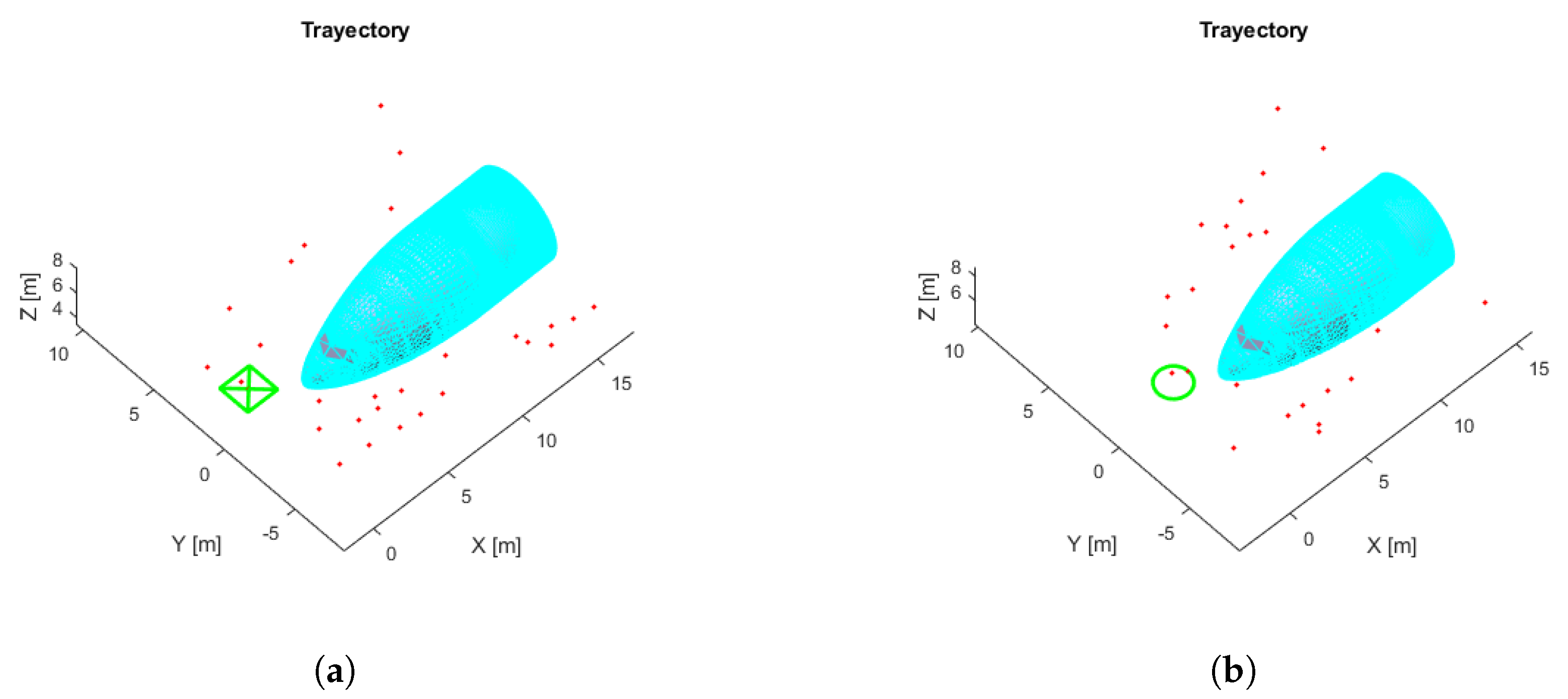
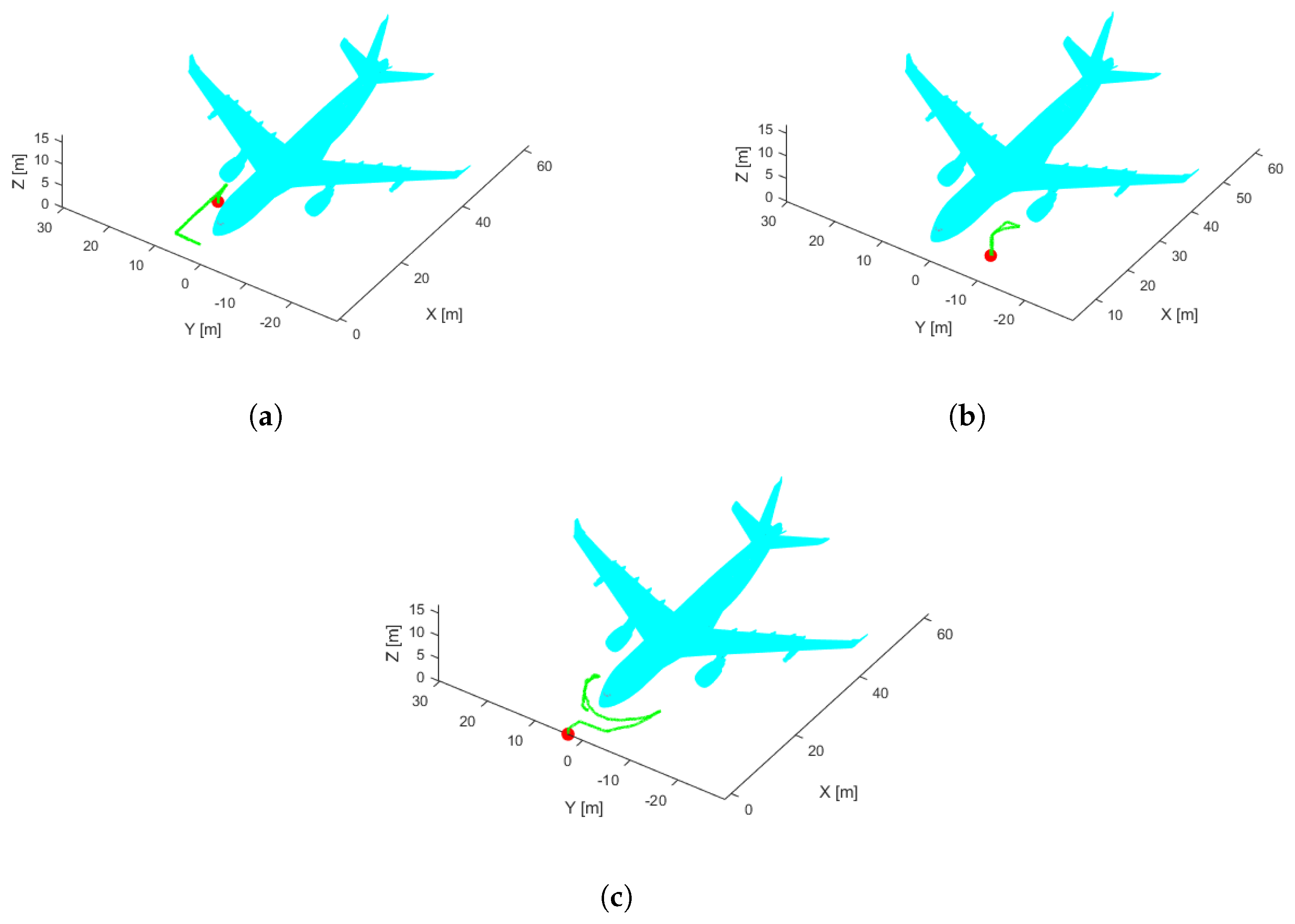
4.5. 3D Localization
4.5.1. Simulation Tests
4.5.2. Real Tests
5. Discussions
5.1. 2D Localization
5.2. 3D Localization
6. Conclusions
6.1. 2D Localization
6.2. 3D Localization
Supplementary Materials
Author Contributions
Funding
Institutional Review Board Statement
Informed Consent Statement
Data Availability Statement
Acknowledgments
Conflicts of Interest
Abbreviations
| UAV | Unmanned Aerial Vehicle |
| CAD | Computer-Aided Design |
| 3D | Three Dimensions |
| 2D | TWO Dimensions |
| UKF | Unscented Kalman Filter |
| EKF | Extended Kalman Filter |
| IMU | Inertial Measurement Units |
| GPS | Global Positioning System |
| ICP | Iterative Closest Point Algorithm |
| ICP-NL | Noun lineal Iterative Closest Point Process |
| NDT | Normal Transformation Distribution |
| SLAM | Simultaneous Localization and Mapping) |
| MCL | Monte Carlo Localization |
| AMCL | Adaptive Monte Carlo Localization |
| ROS | Robot Operative System |
| DAE | Digital Asset Exchange |
| URDF | Unified Robot Description Format |
| ATE | Absolute Trajectory Error |
| MSE | Mean Square Error |
| PCL | Point Cloud Laser Library |
| GT | Ground Truth |
| PC | Personal Computer |
| SVD | Singular Value Decomposition |
| LIDAR | Light Detection and Ranging |
Appendix A. Hummingbird Simulated Odometry Sensor
file: /rotors_simulator/rotors_description/urdf/mav_generic_odometry_sensor.gazebo
mass_odometry_sensor = 0.00001
measurement_divisor = 1
measurement_delay = 0
unknown_delay = 0.0
noise_normal_position = 0 0 0
noise_normal_quaternion = 0 0 0
noise_normal_linear_velocity = 0 0 0
noise_normal_angular_velocity = 0 0 0
noise_normal_position = 0.01 0.01 0.01
noise_normal_quaternion = 0.017 0.017 0.017
noise_uniform_linear_velocity = 0 0 0
noise_uniform_angular_velocity = 0 0 0
enable_odometry_map=false
inertia ixx = 0.00001 ixy = 0.0 ixz = 0.0 iyy = 0.00001 iyz = 0.0 izz = 0.00001 [kg m^2]
origin xyz=0.0 0.0 0.0 rpy=0.0 0.0 0.0
Appendix B. Velodyne VLP16 Simulated 3D Laser Sensor
update rate in hz = 10
samples = 512
minimum range value in meters = 0.9
maximum range value in meters = 130
noise Gausian in meters = 0.008
minimum horizontal angle in radians = -3.14
maximum horizontal angle in radians = 3.14
Appendix C. AMCL Simulations Parameters
odom_model_type value=omni-corrected
 laser_max_beams value=30
 min_particles value=200
 max_particles value=3000
 kld_err value=0.05
 kld_z value=0.99
 odom_alpha1 value=0.2
 odom_alpha2 value=0.2
 odom_alpha3 value=0.8
 odom_alpha4 value=0.2
 odom_alpha5 value=0.2
 laser_likelihood_max_dist value=2
 laser_z_hit value=0.5
 laser_z_short value=0.05
 laser_z_max value=0.05
 laser_z_rand value=0.5
 laser_sigma_hit value=0.2
 laser_lambda_short value=0.1
 laser_model_type value=likelihood_field
 update_min_d value=0.2
 update_min_a value=0.5
 resample_interval value=1
 transform_tolerance value=1.0
 recovery_alpha_slow value=0.001
 recovery_alpha_fast value=0.1
 initial_cov_xx  value=0.5
 initial_cov_yy  value=0.5
 initial_cov_aa  value=0.15
Appendix D. AMCL Real Fligts Parameters
odom_model_type value=omni-corrected
 laser_max_beams value=50
 min_particles value=200
 max_particles value=3000
 kld_err value=0.01
 kld_z value=0.8
 odom_alpha1 value=0.3
 odom_alpha2 value=0.3
 odom_alpha3 value=0.05
 odom_alpha4 value=0.05
 odom_alpha5 value=0.3
 laser_likelihood_max_dist value=0.5
 laser_z_hit value=0.8
 laser_z_short value=0.05
 laser_z_max value=0.05
 laser_z_rand value=0.5
 laser_sigma_hit value=0.2
 laser_lambda_short value=0.1
 laser_model_type value=likelihood_field
 update_min_d value=0.1
 update_min_a value=0.1
 resample_interval value=1
 transform_tolerance value=1.0
 recovery_alpha_slow value=0.001
 recovery_alpha_fast value=0.1
 initial_cov_xx  value=25
 initial_cov_yy  value=25
 initial_cov_aa  value=0.15
References
- Myeong, W.C.; Jung, K.Y.; Jung, S.W.; Jung, Y.; Myung, H. Development of a drone-type wall-sticking and climbing robot. In Proceedings of the 2015 12th International Conference on Ubiquitous Robots and Ambient Intelligence (URAI), Goyangi, Korea, 28–30 October 2015; IEEE: Piscataway, NJ, USA, 2015; pp. 386–389. [Google Scholar]
- Nikolic, J.; Burri, M.; Rehder, J.; Leutenegger, S.; Huerzeler, C.; Siegwart, R. A UAV system for inspection of industrial facilities. In Proceedings of the 2013 IEEE Aerospace Conference, Big Sky, MT, USA, 2–9 March 2013; IEEE: Piscataway, NJ, USA, 2013; pp. 1–8. [Google Scholar]
- Omari, S.; Gohl, P.; Burri, M.; Achtelik, M.; Siegwart, R. Visual industrial inspection using aerial robots. In Proceedings of the 2014 3rd International Conference on Applied Robotics for the Power Industry, Foz do Iguassu, Brazil, 14–16 October 2014; IEEE: Piscataway, NJ, USA, 2014; pp. 1–5. [Google Scholar]
- Menendez, O.A.; Perez, M.; Cheein, F.A.A. Vision based inspection of transmission lines using unmanned aerial vehicles. In Proceedings of the 2016 IEEE International Conference on Multisensor Fusion and Integration for Intelligent Systems, Kongresshaus Baden-Baden, Germany, 19–21 September 2016; IEEE: Piscataway, NJ, USA, 2016; pp. 412–417. [Google Scholar]
- Jiang, W.; Wenkai, F.; Qianru, L. An integrated measure and location method based on airborne 2D laser scanning sensor for UAV’s power line inspection. In Proceedings of the 2013 Fifth International Conference on Measuring Technology and Mechatronics Automation, Hong Kong, China, 16–17 January 2013; IEEE: Piscataway, NJ, USA, 2013; pp. 213–217. [Google Scholar]
- Zhang, J.; Liu, L.; Wang, B.; Chen, X.; Wang, Q.; Zheng, T. High speed automatic power line detection and tracking for a UAV-based inspection. In Proceedings of the 2012 International Conference on Industrial Control and Electronics Engineering, Xi’an, China, 23–25 August 2012; IEEE: Piscataway, NJ, USA, 2012; pp. 266–269. [Google Scholar]
- Alsalam, B.H.Y.; Morton, K.; Campbell, D.; Gonzalez, F. Autonomous UAV with vision based on-board decision making for remote sensing and precision agriculture. In Proceedings of the 2017 IEEE Aerospace Conference, Big Sky, MT, USA, 4–11 March 2017; IEEE: Piscataway, NJ, USA, 2017; pp. 1–12. [Google Scholar]
- Valente, J.; Kooistra, L.; Mücher, S. Fast Classification of Large Germinated Fields Via High-Resolution UAV Imagery. IEEE Robot. Autom. Lett. 2019, 4, 3216–3223. [Google Scholar] [CrossRef]
- Tripicchio, P.; Satler, M.; Dabisias, G.; Ruffaldi, E.; Avizzano, C.A. Towards smart farming and sustainable agriculture with drones. In Proceedings of the 2015 International Conference on Intelligent Environments, Prague, Czech Republic, 15–17 July 2015; IEEE: Piscataway, NJ, USA, 2015; pp. 140–143. [Google Scholar]
- Cerro, J.d.; Cruz Ulloa, C.; Barrientos, A.; de León Rivas, J. Unmanned Aerial Vehicles in Agriculture: A Survey. Agronomy 2021, 11, 203. [Google Scholar] [CrossRef]
- Xi, Z.; Lou, Z.; Sun, Y.; Li, X.; Yang, Q.; Yan, W. A Vision-Based Inspection Strategy for Large-Scale Photovoltaic Farms Using an Autonomous UAV. In Proceedings of the 2018 17th International Symposium on Distributed Computing and Applications for Business Engineering and Science(DCABES), Wuxi, China, 9–23 October 2018; IEEE: Piscataway, NJ, USA, 2018; pp. 200–203. [Google Scholar]
- Stokkeland, M.; Klausen, K.; Johansen, T.A. Autonomous visual navigation of unmanned aerial vehicle for wind turbine inspection. In Proceedings of the 2015 International Conference on Unmanned Aircraft Systems (ICUAS), Denver, CO, USA, 9–12 June 2015; IEEE: Piscataway, NJ, USA, 2015; pp. 998–1007. [Google Scholar]
- Schäfer, B.E.; Picchi, D.; Engelhardt, T.; Abel, D. Multicopter unmanned aerial vehicle for automated inspection of wind turbines. In Proceedings of the 2016 24th Mediterranean Conference on Control and Automation (MED), Athens, Greece, 21–24 June 2016; IEEE: Piscataway, NJ, USA, 2016; pp. 244–249. [Google Scholar]
- Bailey, T.; Durrant-Whyte, H. Simultaneous localization and mapping (SLAM): Part II. IEEE Robot. Autom. Mag. 2006, 13, 108–117. [Google Scholar] [CrossRef] [Green Version]
- Cadena, C.; Carlone, L.; Carrillo, H.; Latif, Y.; Scaramuzza, D.; Neira, J.; Reid, I.; Leonard, J.J. Past, Present, and Future of Simultaneous Localization and Mapping: Toward the Robust-Perception Age. IEEE Trans. Robot. 2016, 32, 1309–1332. [Google Scholar] [CrossRef] [Green Version]
- Avola, D.; Cinque, L.; Fagioli, A.; Foresti, G.L.; Massaroni, C.; Pannone, D. Feature-based SLAM algorithm for small scale UAV with nadir view. In Proceedings of the International Conference on Image Analysis and Processing, Trento, Italy, 9–13 September 2019; Springer: Berlin/Heidelberg, Germany, 2019; pp. 457–467. [Google Scholar]
- Chan, S.H.; Wu, P.T.; Fu, L.C. Robust 2D indoor localization through laser SLAM and visual SLAM fusion. In Proceedings of the 2018 IEEE International Conference on Systems, Man, and Cybernetics (SMC), Miyazaki, Japan, 7–10 October 2018; IEEE: Piscataway, NJ, USA, 2018; pp. 1263–1268. [Google Scholar]
- Luo, Y.; Li, Y.; Li, Z.; Shuang, F. MS-SLAM: Motion State Decision of Keyframes for UAV-Based Vision Localization. IEEE Access 2021, 9, 67667–67679. [Google Scholar] [CrossRef]
- Julier, S.J.; Uhlmann, J.K. New extension of the Kalman filter to nonlinear systems. In Proceedings of the Signal Processing, Sensor Fusion, and Target Recognition VI. International Society for Optics and Photonics, Orlando, FL, United States, 28 July 1997; Volume 3068, pp. 182–193. [Google Scholar]
- Tang, H.; Shen, Z. An attitude estimate method for fixed-wing UAV s using MEMS/GPS data fusion. In Proceedings of the 2017 First International Conference on Electronics Instrumentation & Information Systems (EIIS), Harbin, China, 3–5 June 2017; IEEE: Piscataway, NJ, USA, 2017; pp. 1–5. [Google Scholar]
- Mourikis, A.I.; Roumeliotis, S.I. A multi-state constraint Kalman filter for vision-aided inertial navigation. In Proceedings of the 2007 IEEE International Conference on Robotics and Automation, Roma, Italy, 10–14 April 2007; IEEE: Piscataway, NJ, USA, 2007; pp. 3565–3572. [Google Scholar]
- Wan, E.A.; Van Der Merwe, R. The unscented Kalman filter for nonlinear estimation. In Proceedings of the IEEE 2000 Adaptive Systems for Signal Processing, Communications, and Control Symposium (Cat. No.00EX373), Lake Louise, AB, Canada, 1–4 October 2000; IEEE: Piscataway, NJ, USA, 2000; pp. 153–158. [Google Scholar]
- De Marina, H.G.; Pereda, F.J.; Giron-Sierra, J.M.; Espinosa, F. UAV attitude estimation using unscented Kalman filter and TRIAD. IEEE Trans. Ind. Electron. 2011, 59, 4465–4474. [Google Scholar] [CrossRef] [Green Version]
- Burguera, A.; Oliver, G.; Tardos, J.D. Robust scan matching localization using ultrasonic range finders. In Proceedings of the 2005 IEEE/RSJ International Conference on Intelligent Robots and Systems, Edmonton, AB, Canada, 2–6 August 2005; IEEE: Piscataway, NJ, USA, 2005; pp. 1367–1372. [Google Scholar]
- Fang, H.; Yang, M.; Yang, R. Ground texture matching based global localization for intelligent vehicles in urban environment. In Proceedings of the 2007 IEEE Intelligent Vehicles Symposium, Istanbul, Turkey, 13–15 June 2007; IEEE: Piscataway, NJ, USA, 2007; pp. 105–110. [Google Scholar]
- Nazem, F.; Ahmadian, A.; Seraj, N.D.; Giti, M. Two-stage point-based registration method between ultrasound and CT imaging of the liver based on ICP and unscented Kalman filter: A phantom study. Int. J. Comput. Assist. Radiol. Surg. 2014, 9, 39–48. [Google Scholar] [CrossRef] [PubMed]
- Koide, K.; Miura, J.; Menegatti, E. A portable three-dimensional LIDAR-based system for long-term and wide-area people behavior measurement. Int. J. Adv. Robot. Syst. 2019, 16, 1729881419841532. [Google Scholar] [CrossRef]
- Magnusson, M.; Lilienthal, A.; Duckett, T. Scan registration for autonomous mining vehicles using 3D-NDT. J. Field Robot. 2007, 24, 803–827. [Google Scholar] [CrossRef] [Green Version]
- Sakai, T.; Koide, K.; Miura, J.; Oishi, S. Large-scale 3d outdoor mapping and on-line localization using 3d-2d matching. In Proceedings of the 2017 IEEE/SICE International Symposium on System Integration (SII), Taipei, Taiwan, 11–14 December 2017; IEEE: Piscataway, NJ, USA, 2017; pp. 829–834. [Google Scholar]
- Zhu, H.; Chung, J.J.; Lawrance, N.R.; Siegwart, R.; Alonso-Mora, J. Online informative path planning for active information gathering of a 3d surface. In Proceedings of the 2021 IEEE International Conference on Robotics and Automation (ICRA), Xi’an, China, 30 May–5 June 2021; IEEE: Piscataway, NJ, USA, 2021; pp. 1488–1494. [Google Scholar]
- Fox, D.; Burgard, W.; Thrun, S. Markov localization for mobile robots in dynamic environments. J. Artif. Intell. Res. 1999, 11, 391–427. [Google Scholar] [CrossRef]
- Shoukry, Y.; Abdelfatah, W.F.; Hammad, S.A. Real-time Markov localization for autonomous UGV. In Proceedings of the 2009 4th International Design and Test Workshop (IDT), Riyadh, Saudi Arabia, 15–17 November 2009; IEEE: Piscataway, NJ, USA, 2009; pp. 1–6. [Google Scholar]
- Thrun, S.; Fox, D.; Burgard, W.; Dellaert, F. Robust Monte Carlo localization for mobile robots. Artif. Intell. 2001, 128, 99–141. [Google Scholar] [CrossRef] [Green Version]
- Fox, D.; Burgard, W.; Dellaert, F.; Thrun, S. Monte carlo localization: Efficient position estimation for mobile robots. AAAI/IAAI 1999, 1999, 2. [Google Scholar]
- Xu, S.; Chou, W. An improved indoor localization method for mobile robot based on WiFi fingerprint and AMCL. In Proceedings of the 2017 10th International Symposium on Computational Intelligence and Design (ISCID), Hangzhou, China, 9–10 December 2017; IEEE: Piscataway, NJ, USA, 2017; Volume 1, pp. 324–329. [Google Scholar]
- Javierre, P.; Alvarado, B.P.; de la Puente, P. Particle filter localization using visual markers based omnidirectional vision and a laser sensor. In Proceedings of the 2019 Third IEEE International Conference on Robotic Computing (IRC), Naples, Italy, 25–27 February 2019; IEEE: Piscataway, NJ, USA, 2019; pp. 246–249. [Google Scholar]
- Yilmaz, A.; Temeltas, H. Self-adaptive Monte Carlo method for indoor localization of smart AGVs using LIDAR data. Robot. Auton. Syst. 2019, 122, 103285. [Google Scholar] [CrossRef]
- Siegel, M.; Gunatilake, P.; Podnar, G. Robotic assistants for aircraft inspectors. IEEE Instrum. Meas. Mag. 1998, 1, 16–30. [Google Scholar] [CrossRef]
- Rice, M.; Li, L.; Ying, G.; Wan, M.; Lim, E.T.; Feng, G.; Ng, J.; Teoh Jin-Li, M.; Babu, V.S. Automating the visual inspection of aircraft. In Proceedings of the Singapore Aerospace Technology and Engineering Conference (SATEC), Suntec, Singapur, 7 February 2018. [Google Scholar]
- Ramalingam, B.; Manuel, V.H.; Elara, M.R.; Vengadesh, A.; Lakshmanan, A.K.; Ilyas, M.; James, T.J.Y. Visual inspection of the aircraft surface using a teleoperated reconfigurable climbing robot and enhanced deep learning technique. Int. J. Aerosp. Eng. 2019, 2019, 5137139. [Google Scholar] [CrossRef]
- Donadio, F.; Frejaville, J.; Larnier, S.; Vetault, S. Human-robot collaboration to perform aircraft inspection in working environment. In Proceedings of the 5th International Conference on Machine Control and Guidance (MCG), Vichy, France, 5–6 October 2016. [Google Scholar]
- Blokhinov, Y.B.; Gorbachev, V.; Nikitin, A.; Skryabin, S. Technology for the Visual Inspection of Aircraft Surfaces Using Programmable Unmanned Aerial Vehicles. J. Comput. Syst. Sci. Int. 2019, 58, 960–968. [Google Scholar] [CrossRef]
- Miranda, J.; Larnier, S.; Herbulot, A.; Devy, M. UAV-based inspection of airplane exterior screws with computer vision. In Proceedings of the 14h International Joint Conference on Computer Vision, Imaging and Computer Graphics Theory and Applications, Prague, Czech Republic, 25–27 February 2019. [Google Scholar]
- Hornung, A.; Wurm, K.M.; Bennewitz, M.; Stachniss, C.; Burgard, W. OctoMap: An Efficient Probabilistic 3D Mapping Framework Based on Octrees. Auton. Robot. 2013, 34, 189–206. [Google Scholar] [CrossRef] [Green Version]
- Jian, X. Occupancy Grids Maps for Localization and Mapping. In Motion Planning; Intech: London, UK, 2008; pp. 381–406. [Google Scholar]
- Thrun, S.; Montemerlo, M. The graph SLAM algorithm with applications to large-scale mapping of urban structures. Int. J. Robot. Res. 2006, 25, 403–429. [Google Scholar] [CrossRef]
- Fox, D.; Burgard, W.; Thrun, S. Grid and Monte Carlo Localization. In Probalistic Robotics; Early Draft; 2000; pp. 187–219. Available online: https://docs.ufpr.br/~danielsantos/ProbabilisticRobotics.pdf (accessed on 11 April 2022)Early Draft.
- Fantoni, S.; Castellani, U.; Fusiello, A. Accurate and automatic alignment of range surfaces. In Proceedings of the 2012 Second International Conference on 3D Imaging, Modeling, Processing, Visualization Transmission, Zurich, Switzerland, 13–15 October 2012; IEEE: Piscataway, NJ, USA, 2012; pp. 73–80. [Google Scholar]
- Rusu, R.B.; Cousins, S. 3d is here: Point cloud library (pcl). In Proceedings of the 2011 IEEE International Conference on Robotics and Automation, Shanghai, China, 9–13 May 2011; IEEE: Piscataway, NJ, USA, 2011; pp. 1–4. [Google Scholar]
- Besl, P.J.; McKay, N.D. Method for registration of 3-D shapes. In Proceedings of the Sensor Fusion IV: Control Paradigms and Data Structures, Boston, MA, United States, 30 April 1992; International Society for Optics and Photonics: Bellingham, WA, USA, 1992; Volume 1611, pp. 586–606. [Google Scholar]
- Ros. Available online: https://www.ros.org/ (accessed on 11 April 2022).
- Gazebo Robot Simulation. Available online: http://gazebosim.org/ (accessed on 11 April 2022).
- Aerostack. Available online: https://github.com/cvar-upm/aerostack/wiki (accessed on 11 April 2022).
- Furrer, F.; Burri, M.; Achtelik, M.; Siegwart, R. Robot Operating System (ROS): The Complete Reference (Volume 1); Chapter RotorS—A Modular Gazebo MAV Simulator Framework; Springer: Cham, Switzerland, 2016; pp. 595–625. [Google Scholar] [CrossRef]
- Velodyne Simulator. Available online: https://bitbucket.org/DataspeedInc/velodyne_simulator/src/master/ (accessed on 11 April 2022).
- Moore, T.; Stouch, D. A Generalized Extended Kalman Filter Implementation for the Robot Operating System. In Proceedings of the 13th International Conference on Intelligent Autonomous Systems (IAS-13), Padova, Italy, 15–18 July 2014; Springer: Berlin/Heidelberg, Germany, 2014. [Google Scholar]
- Airbus Cad Model. Available online: https://www.thingiverse.com/thing:847897 (accessed on 11 April 2022).
- Aircraft Airbus. Available online: https://commons.wikimedia.org/wiki/File:Arrival_of_Iran_Air_Airbus_A330-200_%28EP-IJA%29_at_Mehrabad_International_Airport_%2812%29.jpg (accessed on 11 April 2022).
- Sturm, J.; Engelhard, N.; Endres, F.; Burgard, W.; Cremers, D. A benchmark for the evaluation of RGB-D SLAM systems. In Proceedings of the 2012 IEEE/RSJ International Conference on Intelligent Robots and Systems, Vilamoura-Algarve, Portugal, 7–12 October 2012; IEEE: Piscataway, NJ, USA, 2012; pp. 573–580. [Google Scholar]
- Absolute Trajectory Error. Available online: http://www.rawseeds.org/rs/methods/view/9l (accessed on 11 April 2022).
- Anagnostopoulos, I.; Pătrăucean, V.; Brilakis, I.; Vela, P. Detection of walls, floors, and ceilings in point cloud data. In Proceedings of the Construction Research Congress 2016, San Juan, Puerto Rico, 31 May–2 June 2016; pp. 2302–2311. [Google Scholar]
- Chum, O.; Matas, J.; Kittler, J. Locally optimized RANSAC. In Proceedings of the Joint Pattern Recognition Symposium, Magdeburg, Germany, 10–12 September 2003; Springer: Berlin/Heidelberg, Germany, 2003; pp. 236–243. [Google Scholar]
- Point Cloud Library. Available online: https://pcl.readthedocs.io/projects/tutorials/en/latest/planar_segmentation.html#planar-segmentation (accessed on 11 April 2022).
- Montemerlo, M.; Thrun, S.; Koller, D.; Wegbreit, B. FastSLAM: A factored solution to the simultaneous localization and mapping problem. AAAI/IAAI 2002, 593598. Available online: https://www.aaai.org/Papers/AAAI/2002/AAAI02-089.pdf (accessed on 11 April 2022).


| Altitude (m) | 3 | 4 | 5 | 6 | 7 | 8 |
|---|---|---|---|---|---|---|
| Mean ATE (m) | 0.3460 | 0.3287 | 0.3127 | 0.3376 | 0.4077 | 2.1437 |
| Tests | ATE Min (m) | Ate Max (m) | Mean ATE (m) |
|---|---|---|---|
| 81 | 0.18 | 5.63 | 0.34 |
| ATE | GT Initial Pos (x,y) (m) | AMCL Initial Pos (x,y) (m) | Initial Covariance (xx,yy) (m) | Initial Error (x,y) (m) |
|---|---|---|---|---|
| Min ATE 0.18 | 32.53, −27.83 | 32.91, −27.5 | 0.5, 0.5 | −0.38, −0.33 |
| Max ATE 5.63 | 33.72, −29 | 36.01, −26.56 | 0.5, 0.5 | −2.29, −2.44 |
| Error between AMCL and Ground Truth (m) | Mean Covariance(x,y) | Mean Occupancy Grip Map | Mean 2D Laser Scan | Mean Relation Matches/Laser-Scan |
|---|---|---|---|---|
| <=0.3 | 0.0557 | 41,820 | 245,917.5 | 0.17005 |
| ATE | GT Initial Pos (x,y) (m) | AMCL Initial Pos (x,y) (m) | Initial Covariance (xx,yy) (m) | Initial Error (x,y) (m) |
|---|---|---|---|---|
| Min ATE 0.86 | 20.66, 7.16 | 20.77 , 5.56 | 0.5, 0.5 | −0.11, −1.6 |
| Max ATE 1.4 | −4.82, −5 | −4.77, −4.6 | 0.5, 0.5 | −0.05, −0.4 |
| Error between AMCL and Ground Truth (m) | Mean Covariance (x,y) | Mean Occupancy Grip Map | Mean 2D Laser Scan | Mean Relation Matches/Laser-Scan |
|---|---|---|---|---|
| <=0.3 | 0.0115 | 18,037 | 76,847 | 0.2347 |
| Algorithm | ATE |
|---|---|
| ICP-NL | 0.68 |
| NDT | 289.93 |
| Algorithm | Height (m) | ATE (m) | Convergence Time (s) |
|---|---|---|---|
| ICP-NL | 3.5 | 0.7265 | 2.3 |
| 4.5 | 0.7077 | 2.8 | |
| 5.5 | 0.7442 | 4 | |
| 6.5 | 0.6857 | 3.1 | |
| 7.5 | 0.6334 | 1.6 | |
| 8.5 | 0.552 | 4.1 | |
| NDT | 3.5 | 149.6588 | 181.4 |
| 4.5 | 511.6744 | 57.7 | |
| 5.5 | 363.2043 | 103.3 | |
| 6.5 | 133.5604 | 50.9 | |
| 7.5 | 0.6597 | 7 | |
| 8.5 | 1.6485 | 21.5 |
| Algorithm | Height (m) | ATE (m) | Convergence Time (s) |
|---|---|---|---|
| ICP-NL | 2.5 | 0.3801 | 2.3 |
| 3.5 | 0.5552 | 2.8 | |
| 4.5 | 0.5442 | 4 | |
| 5.5 | 0.6857 | 3.1 |
Publisher’s Note: MDPI stays neutral with regard to jurisdictional claims in published maps and institutional affiliations. |
© 2022 by the authors. Licensee MDPI, Basel, Switzerland. This article is an open access article distributed under the terms and conditions of the Creative Commons Attribution (CC BY) license (https://creativecommons.org/licenses/by/4.0/).
Share and Cite
Espinosa Peralta, P.; Luna, M.A.; de la Puente, P.; Campoy, P.; Bavle, H.; Carrio, A.; Cruz Ulloa, C. Performance Analysis of Localization Algorithms for Inspections in 2D and 3D Unstructured Environments Using 3D Laser Sensors and UAVs. Sensors 2022, 22, 5122. https://doi.org/10.3390/s22145122
Espinosa Peralta P, Luna MA, de la Puente P, Campoy P, Bavle H, Carrio A, Cruz Ulloa C. Performance Analysis of Localization Algorithms for Inspections in 2D and 3D Unstructured Environments Using 3D Laser Sensors and UAVs. Sensors. 2022; 22(14):5122. https://doi.org/10.3390/s22145122
Chicago/Turabian StyleEspinosa Peralta, Paul, Marco Andrés Luna, Paloma de la Puente, Pascual Campoy, Hriday Bavle, Adrián Carrio, and Christyan Cruz Ulloa. 2022. "Performance Analysis of Localization Algorithms for Inspections in 2D and 3D Unstructured Environments Using 3D Laser Sensors and UAVs" Sensors 22, no. 14: 5122. https://doi.org/10.3390/s22145122