2.3.1. Density
According to [
42,
43], ultrasonic methods can determine the density
of a fluid through the use of the Newton–Laplace Equation (
2) and measurement of the speed of sound in that medium.
where
is the isentropic (adiabatic) compressibility of the fluid and
c is the speed of sound at this fluid. Usually, the compressibility is also expressed in terms of its reciprocal, i.e., the bulk modulus
[
32,
44].
The speed of sound can be obtained either through a pulse-echo system [
45] or through a system of two transducers (emitter–receiver) [
46,
47]. Both principles are based on the measurement of the wave propagation time in the fluid, differing only in the number of ultrasonic transducers used.
In case of a pulse-echo system, the basic principle involves the use of an ultrasonic transducer that outputs a very short pulsed signal of the proper ultrasonic frequency. The ultrasonic wave travels through the propagation medium to the other side, where a reflector material is positioned. Hence, there is a reflection of this ultrasonic wave, causing a large part of the energy of the ultrasonic wave to return through the medium to the transducer that emitted it.
In case of an emitter–receiver system, there are two transducers positioned on separate sides forming an acoustic trajectory between them. While one ultrasonic transducer emits, the other receives the ultrasonic signal that has propagated through the measurement medium.
In the proposed system, multiple acoustic trajectories are used, as illustrated in
Figure 4. In the figure, two transducers are opposed at the conduit and form an acoustic trajectory of length
L and angle
with the conduit wall. During transmission, the ultrasonic pulse that travels in favor of the fluid flow through the conduit (in downstream direction) travels the distance
L in a time period
smaller than the pulse that travels in the opposite direction (against the fluid flow, in upstream direction) in a time
.
Considering that, in
Figure 4,
is the axial velocity of the fluid flowing through the conduit (whose amplitude has a value of
), its projection on the trajectory
L (at an angle
with the flow direction) is given by
. Hence, whenever there is a fluid flowing through the conduit, the speed of the ultrasonic pulses downstream (
) and upstream (
) can be calculated as (
3) and (
4), respectively.
In addition, the propagation times of the ultrasonic pulses downstream (
) and upstream (
) can be calculated as (
5) and (
6), respectively.
Combining Equations (
5) and (
6), it can be shown that the speed of ultrasonic wave
c can be obtained as a function of the downstream and upstream travel times as per Equation (
7).
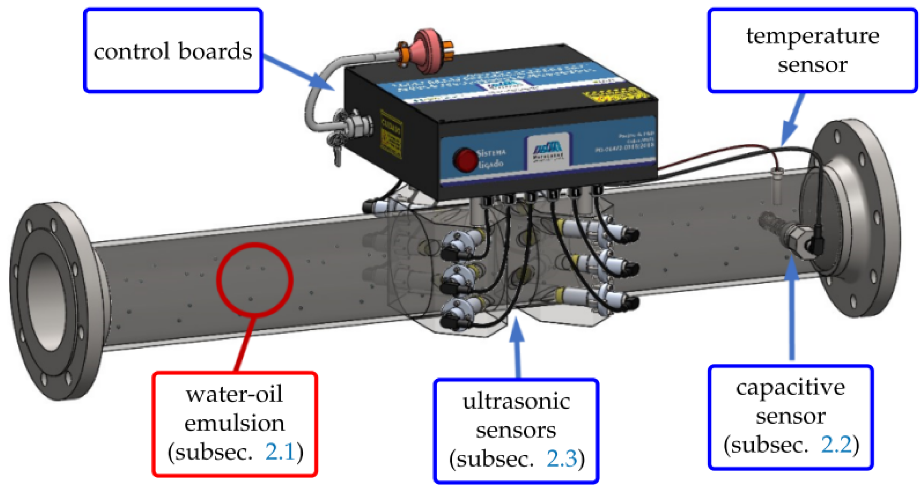
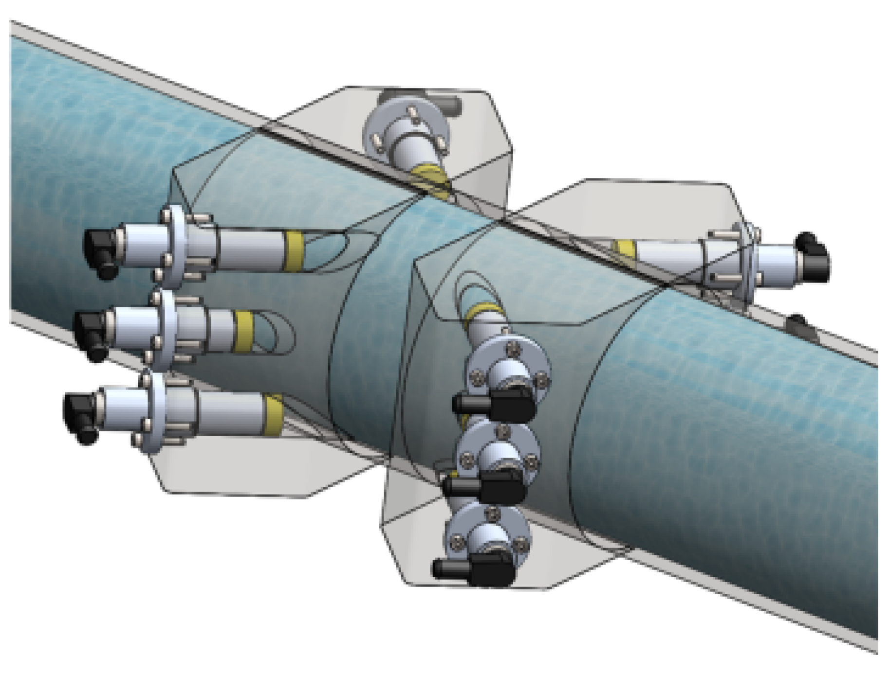
As presented in
Figure 1, the ultrasonic system has three layers of planes equivalent to
Figure 4, and each layer has two crossed ultrasonic trajectories. Hence, Equation (
7) can be modified to (
8), in order to obtain an average velocity
considering each of the six trajectories
and each of the six pairs of downstream and upstream times (
and
, respectively).
where
i is an index corresponding to one of the six trajectories.
The technique used to measure the ultrasonic wave propagation times is based on the zero-crossing detection [
48] of the pulses at the receivers.
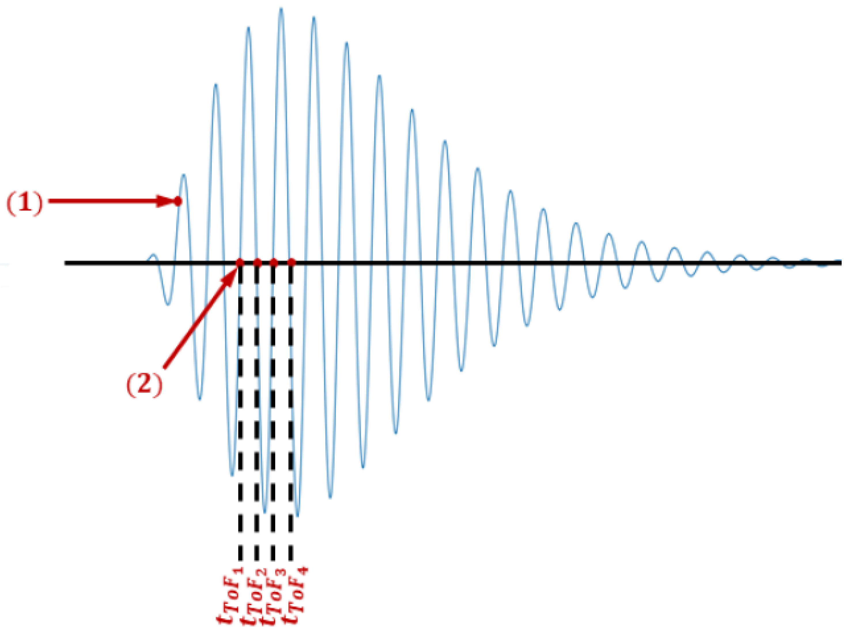
Figure 5 presents the detection of the zero-crossing of an ultrasonic wave. After the transmission of the ultrasonic pulse, the FPGA starts counting the time of several zero-crossings at the receiver. In order to avoid any initial transient, the first cycles are skipped. This is performed by detecting a pre-defined threshold (indicated by (1) in the figure). After the threshold, more three zero-crossings are skipped (until the first valid zero-crossing, indicated by (2) at the figure). Then the time from the starting of the pulse until next
M number of zero-crossings (
until
) are computed. The average time of the valid zero crossings is calculated (recursively) using Equation (
9).
where
is the average of the zero crossing times. It is important to note that
can be any of the
or
times in Equation (
8). Furthermore,
is the average time of the half cycle of oscillation of the signal, and is calculated with (
10).
Finally, the average speed of the ultrasound waves (calculated as (
8)) at the fluid is used in Equation (
2) in order to obtain the density
of the fluid.
2.3.2. Flow Rate
According with [
49,
50], the flow rate
using multiple acoustic trajectories arranged at different heights in the cross section of the conduit can be calculated as (
11). This calculation performs a numerical integration of
N trajectories arranged in distinct heights in the cross section of the penstock. The most used integration methods [
51] are: Gauss–Legendre (for rectangular sections) and Gauss–Jacobi (for circular sections). The OWICS (Optimal Weighted Integration, for circular sections) and the OWIRS (Optimal Weighted Integration for rectangular sections) [
48] can also be highlighted. What differentiates the methods are the speed profiles [
49,
52], whereas the Gauss–Legendre and the Gauss–Jacobi propose uniform speed profiles [
51].
where
is the position of the trajectory in relation to the cross section of the conduit.
is the average axial speed along trajectory
i, calculated according to Equation (
12).
are weighting coefficients (which depend on the number of trajectories and on the integration technique in use, according to Equation (
13)).
D is the dimension of the parallel conduit for the intersection of two acoustic planes (i.e., the diameter of a circular section conduit).
N is the total number of acoustic trajectories in a measurement plane.
is the distance (length) of the acoustic trajectory
i, and
is the angle between the acoustic trajectories.
where
is the measured propagation time upstream and
is the measured propagation time downstream. Their difference is known as
.
According to [
49,
51], the weighting coefficients can be calculated as (
13).
where the parameter
is dependent on the type of integration used (
for the Gauss–Legendre method and
for the OWICS method, considering circular cross-section conduits in both cases). The variable
is the Lagrange polynomial integration, calculated as (
14).
The developed system was based on a measurement configuration using six acoustic trajectories introduced in a circular spool, as presented in
Figure 6. The acoustic trajectories are distributed in two crossed measurement planes (
A and
B), containing three trajectories in each plane. Therefore, the flow rate for a measurement plan (
A or
B) is determined from Equation (
11) and results in (
15). Furthermore, each sensor forms an angle of
with the conduit wall.
Using (
15) for both planes
A and
B, the resultant flow rate can be obtained as the average (
16).
Each of the two planes has a trajectory positioned at the center of the circular spool and two other trajectories equidistant from the center, forming the positions
,
and
. For each trajectory, based on Equations (
13) and (
14), the respective weights
are presented in
Table 2, either considering Gauss–Jacobi or OWICS integration methods.
Table 3 presents the measured lengths (
) of the trajectories for either planes
A and
B. Ideally, the lengths
and
of both planes should have the same value, as well as the lengths
of both planes. However, due to a not so precise drilling, there are these 1 mm discrepancies.
2.3.3. Evaluation Setup
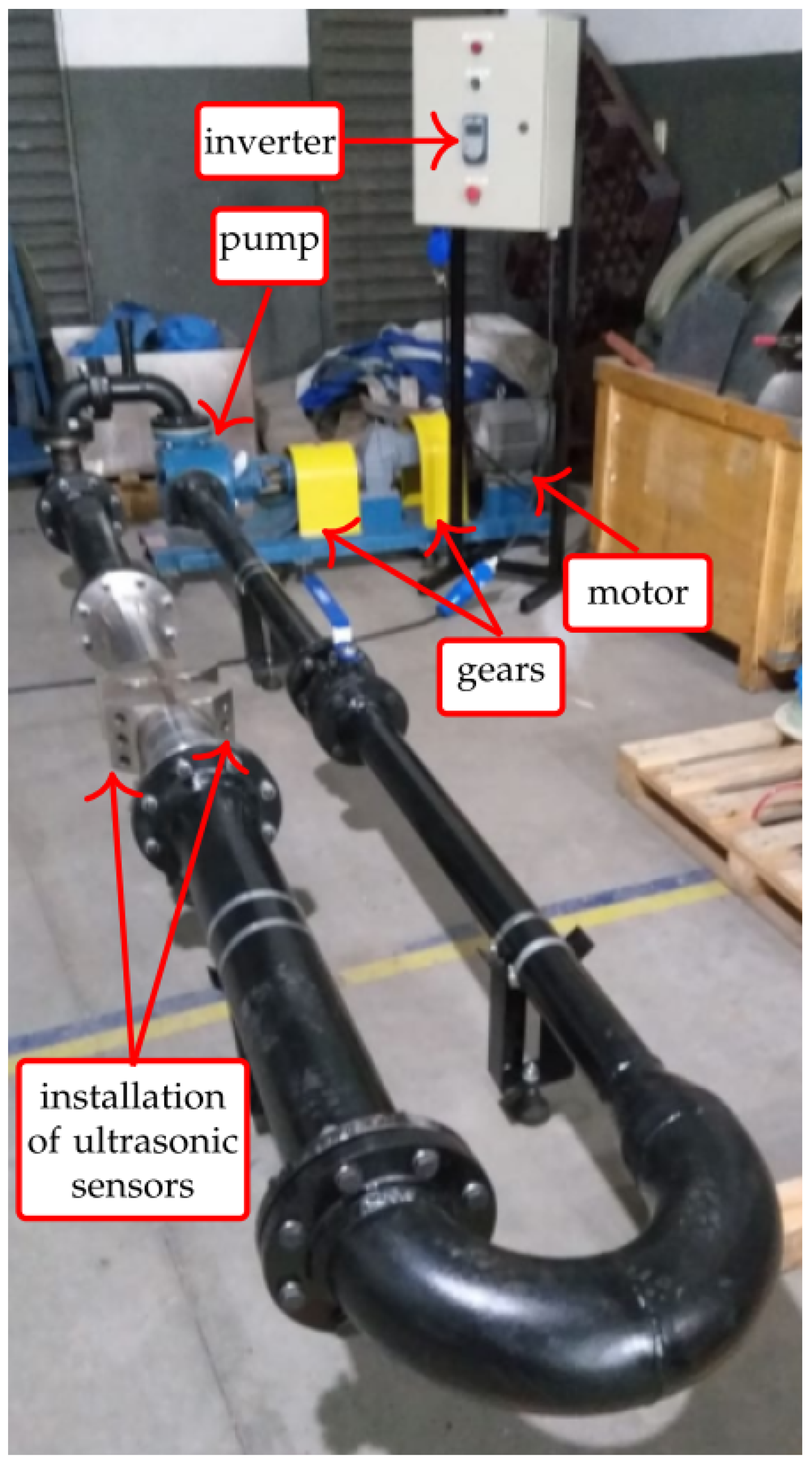
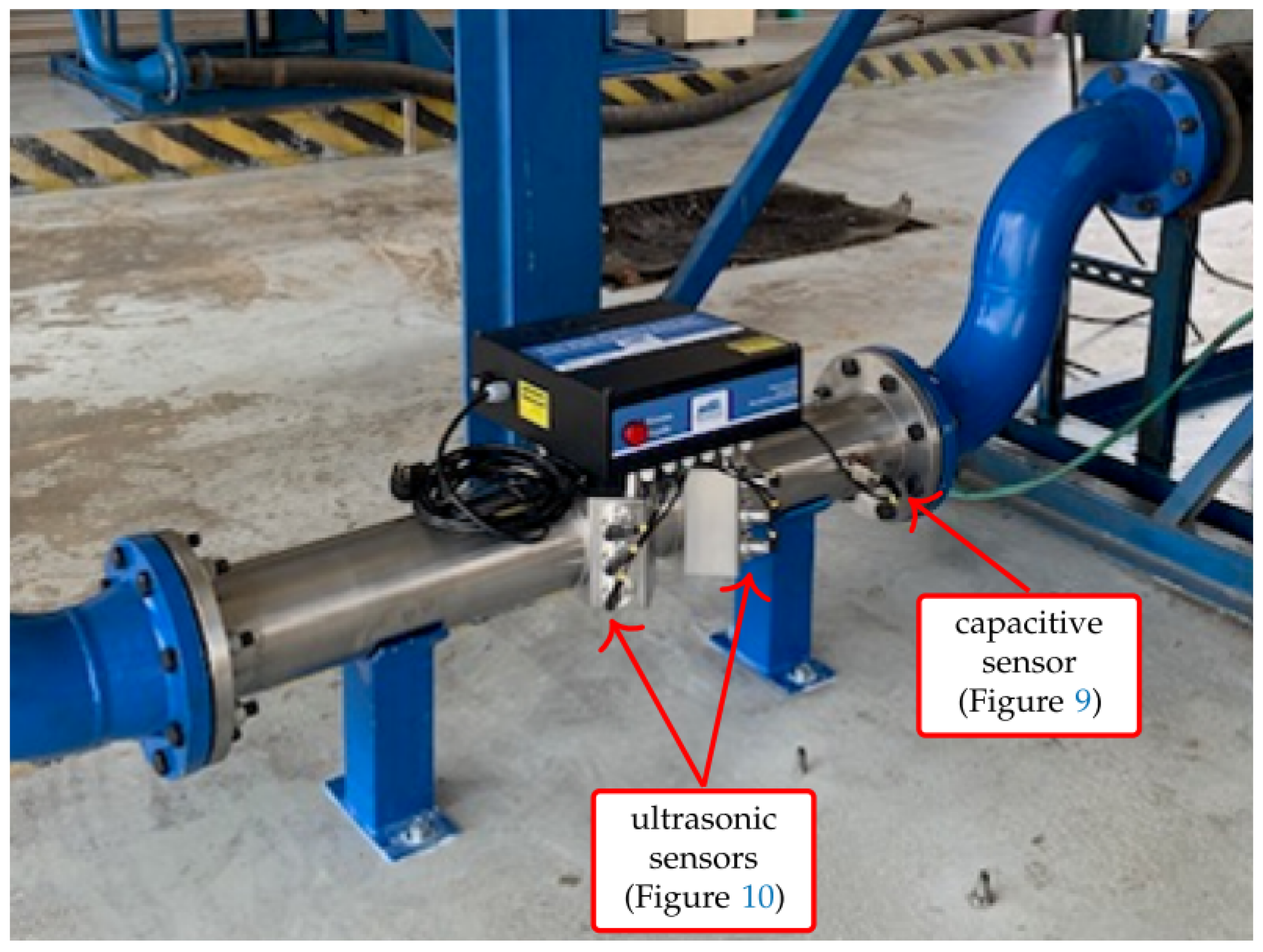
In order to evaluate the ultrasonic system, a reduced scale flow setup has been assembled, as presented in
Figure 7. This setup is formed by a pump driven by an electric motor (whose speed is controlled by an inverter) and a closed loop hydraulic system.
With the setup of
Figure 7, it was possible to vary the flow of the hydraulic circuit by controlling the rotation of the motor that drives the pump. In total, five motor speeds were used (0 RPM, 450 RPM, 500 RPM, 600 RPM, and 700 RPM) in order to achieve a more stable flow in the system. The motor speeds are reduced to the pump using a gear train (of ratio 2.54).
Water has been used as the circulating fluid, as it is it is cheaper than oil and its physical–chemical parameters are well known in the literature. For each motor speed, 100 complete transit time measurements were acquired for each of the 12 trajectories. Means and standard deviations were calculated from the measurements taken, as well as the uncertainties associated with the measurement.
Evaluation of Flow Measurements
Table 4 presents the obtained flows (measured with the ultrasonic system) for each motor rotation (as well as the respective pump rotations).
Ideally, the flow measurements obtained with the proposed sensors should be validated using a certified flow measurement system. As this was not possible, the solution found was to compare the measured flows against the data sheet of the pump [
53], which relates flow with pump rotation. From the data of
Table 4, a linear regression is performed, resulting in the Equation (
17).
where
is the motor rotation (in RPM) and
is the interpolated flow (in m
/h) measured with the prototype.
The manufacturer curve of the pump can be obtained in [
53] and results in Equation (
18).
where
is the reference flow (in m
/h) for a motor rotation
.
Based on Equations (
17) and (
18), for some values of motor rotation, the flows of the proposed system can be compared against the theoretical flows at the pump. This comparison is presented in
Table 5.
Evaluation of Speed-of-Sound and Density Measurements
As the fluid used in the evaluation setup was water, and the fluid temperature at the moment of the tests was 19.40
C, and the value of speed of sound can be obtained as 1480.36 m/s [
54] and the value of density can be obtained as 998.34 kg/m
[
55]. These theoretical values can be used in order to validate the measurements of speed of sound and density performed with the proposed prototype. These comparisons are presented in
Table 6 and
Table 7.


 ,
, 


