A 10-Year Cloud Fraction Climatology of Liquid Water Clouds over Bern Observed by a Ground-Based Microwave Radiometer

Abstract

Cloud fraction (CF) is known as the dominant modulator of Earth’s radiative fluxes. Ground-based CF observations are useful to characterize the cloudiness of a specific site and are valuable for comparison with satellite observations and numerical models. We present for the first time CF statistics (relative to liquid clouds only) for Bern, Switzerland, derived from the observations of a ground-based microwave radiometer. CF is derived with a new method involving the analysis of the integrated liquid water distribution measured by the radiometer. The 10-year analyzed period (2004–2013) allowed us to compute a CF climatology for Bern, showing a maximum CF of 60.9% in winter and a minimum CF of 42.0% in summer. The CF monthly anomalies are identified with respect to the climatological mean values, and they are confirmed through MeteoSwiss yearly climatological bulletins. The CF monthly mean variations are similar to the observations taken at another Swiss location, Payerne, suggesting a large-scale correlation between different sites on the Swiss Plateau. A CF diurnal cycle is also computed, and large intraseasonal variations are found. The overall mean CF diurnal cycle, however, shows a typical sinusoidal cycle, with higher values in the morning and lower values in the afternoon.

1. Introduction

The importance of cloud fraction (CF) in the modulation of Earth’s radiative fluxes has been demonstrated both theoretically and experimentally. A mere 4% increase in the area of the globe covered by low-level stratus clouds would be sufficient to offset the 2–3 K predicted rise in global temperature due to a doubling of CO₂ [1]. CF is used in climate models to determine the radiative fluxes through the atmosphere and at the surface. With increasing CF, all-sky shortwave cloud radiative forcing decreases, and longwave cloud radiative forcing increases [2,3]. CF statistics are also useful for the choice of a suitable site for astronomical observations [4] or for the installation of solar power plants.

CF can be measured by ground-based instruments or by satellite observations. Several ground-based studies about CF have been conducted using observations at the Atmospheric Radiation Measurement (ARM) Program Southern Great Plains (SGP) site in Oklahoma, United States [2,3,5–10], a research facility characterized by a long series of measurements (since 1997) and the presence of multiple instruments (cloud radars, lidars and ceilometers) [8]. Other common sites for the analysis of ground-based CF observations are the North Slope of Alaska (NSA) [3,7,11] and the Tropical Western Pacific (TWP) [7]. The satellite CF observations are often compared with the CF observed at the ground, and instruments onboard both polar and geostationary satellites have been used [5,6,10,12]. Satellite observations allow the analysis of CF for larger areas and for regions not covered by surface observations, as done by Butt et al. [12] for Amazonia, by Pfeifroth et al. [13] for Europe and Africa and by Min and Zhang [14] for the southeast Atlantic. There are also studies comparing surface or satellite CF observations with global or regional numerical models [7,13] or comparing surface CF observations with reanalysis datasets [11].

In recent years, the Swiss Global Climate Observing System (GCOS) Office of the Federal Office of Meteorology and Climatology MeteoSwiss has published two studies comparing several years of CF observations from the Terra and Aqua satellites with CF observations at different Synop (synoptic) stations in Switzerland [15,16]. The purpose of these studies was to improve and complement the long-term, high-quality ground-based observations of cloud properties in Switzerland through the use of satellite-based products. The Terra and Aqua satellites provide a high spatial resolution (0.05°), but at the expense of a lower temporal resolution (up to four daytime overpasses over Switzerland). The Synop observations, on the other hand, are localized, but performed more often (every three hours). Yet, these Synop observations cannot compare with the temporal resolution of cloud radars, lidars and ceilometers (typically 10 s [8]). The latter instruments are therefore better for detecting the hourly variations of the CF diurnal cycle. Furthermore, the reliability of the seasonal CF variations also depends on the continuity of the measurements. For example, the monthly mean CF shown in Seiz et al. [15] is biased towards daytime values, because the satellite CF observations used for the comparison with surface observations were performed only during daytime.

In this study, we present a 10-year CF climatology relative to liquid clouds for Bern, Switzerland, derived from the high-resolution observations (7–11 s) of a ground-based microwave radiometer for the period 2004–2013. CF observations with microwave radiometers are unusual, as they are normally employed to retrieve profiles or integrated values of water vapor and cloud liquid water or temperature profiles [17,18]. We developed, however, a method to derive CF from the integrated cloud liquid water distribution.

The advantage of using a microwave radiometer for CF computation is that it is not affected by the limitations of the other techniques. Synoptic reports are subjective and difficult during nighttime; ground-based active instruments are affected by significant instrument downtime that limits available samples and increases observational errors; and satellite measurements are often biased during nighttime, because they use a combination of visual and infrared radiances. The continuous measurements of the radiometer allowed us to characterize with high confidence the seasonal and diurnal CF variations averaged over 10 years at this Swiss location and to detect the anomalies relative to individual months, as well.

This paper is organized as follows: in Section 2, we describe the instrument and the method used to derive the CF; in Section 3, we present the 10-year CF climatology, the CF monthly anomalies and the CF diurnal cycle; in Section 4, we summarize our findings and give an outlook on future work.

2. Experimental Section

2.1. The TROWARA Radiometer

In this study, we use the measurements provided by the Tropospheric Water Radiometer (TROWARA), a dual-channel microwave radiometer built by Peter and Kämpfer [19], capable of measuring vertically-integrated water vapor (IWV) and vertically-integrated cloud liquid water (ILW, also known as liquid water path (LWP)). TROWARA is located inside a temperature-controlled room on the roof of the Exakte Wissenschaften (Physics and Mathematics) building, University of Bern (46.951° N, 7.439° E, 575 m a.s.l.) and has been operated since the end of 1994, providing an almost uninterrupted series of measurements. The two microwave channels are centered at 21.4 GHz (bandwidth 100 MHz) and 31.5 GHz (bandwidth 200 MHz), the lower frequency being more sensitive to water vapor emission and the higher frequency more sensitive to liquid water emission. An additional infrared channel (λ = 9.5–11.5 μm) is used to determine the temperature of the cloud base. TROWARA’s antenna has a full width at half power of 4° at both frequencies and is pointing to the sky at an elevation angle of 40° towards the southeast.

The current technique used to retrieve IWV and ILW is based on measuring the brightness temperature in the two microwave channels and computing the corresponding zenith opacities (see Equation (2) of Mätzler and Morland [18]). IWV and ILW are then given by a linear combination of the zenith opacities (see Equations (6) and (8) of Mätzler and Morland [18]). The uncertainties declared by Peter and Kämpfer [19] are 3% of the measured value for IWV and 10%–20% of the measured value for ILW (ILW > 0.1 mm). In addition to the relative error, there was a zero bias error for ILW of the order of 0.01–0.02 mm. The physical retrieval of Mätzler and Morland [18], by using a new dielectric model of water, which implements the measured cloud temperature, improved the ILW zero bias error to 0.001 mm [18].

TROWARA’s measurements are accurate for non-precipitating conditions. During rainy events, the microwave emission of the cloud droplets is outmatched by the much greater emission coming from the rain droplets, and a proper determination of ILW is no longer possible. Mätzler [20] found that the ILW values of non-raining clouds normally do not exceed 0.4 mm. For rain events, we therefore assign to ILW a maximum value of 0.4 mm. A second shortcoming of TROWARA is that it is not able to detect ice clouds, such as cirrus clouds, due to the negligible ice absorption in the microwave region.

For this study, we consider ILW only (thus, not presenting the results relative to IWV), and we select a 10-year period between 01 January 2004 and 31 December 2013. The most recent half of the whole ILW time series available was chosen for this analysis, because it contains the most accurate data, due to the relatively recent hardware improvements [21,22] and to the absence of extended data gaps, particularly present in the years before 2003. This 10-year period is still long enough to derive a monthly climatology of the CF variations. The sampling time during this period is on average 11 s until 07 October 2009 and 6.8 s afterwards. The reason for the change is an upgrade of the instrument computer.

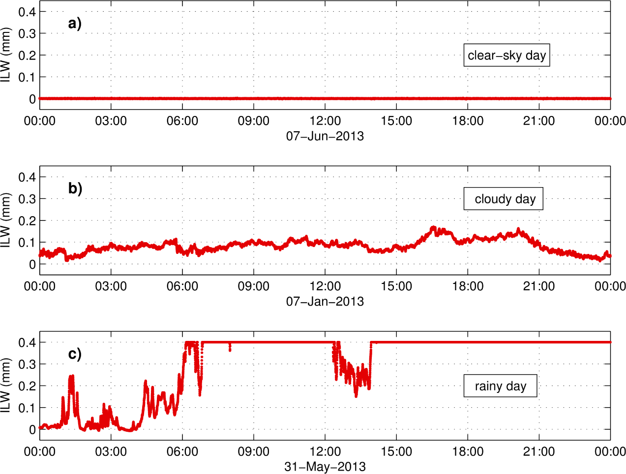
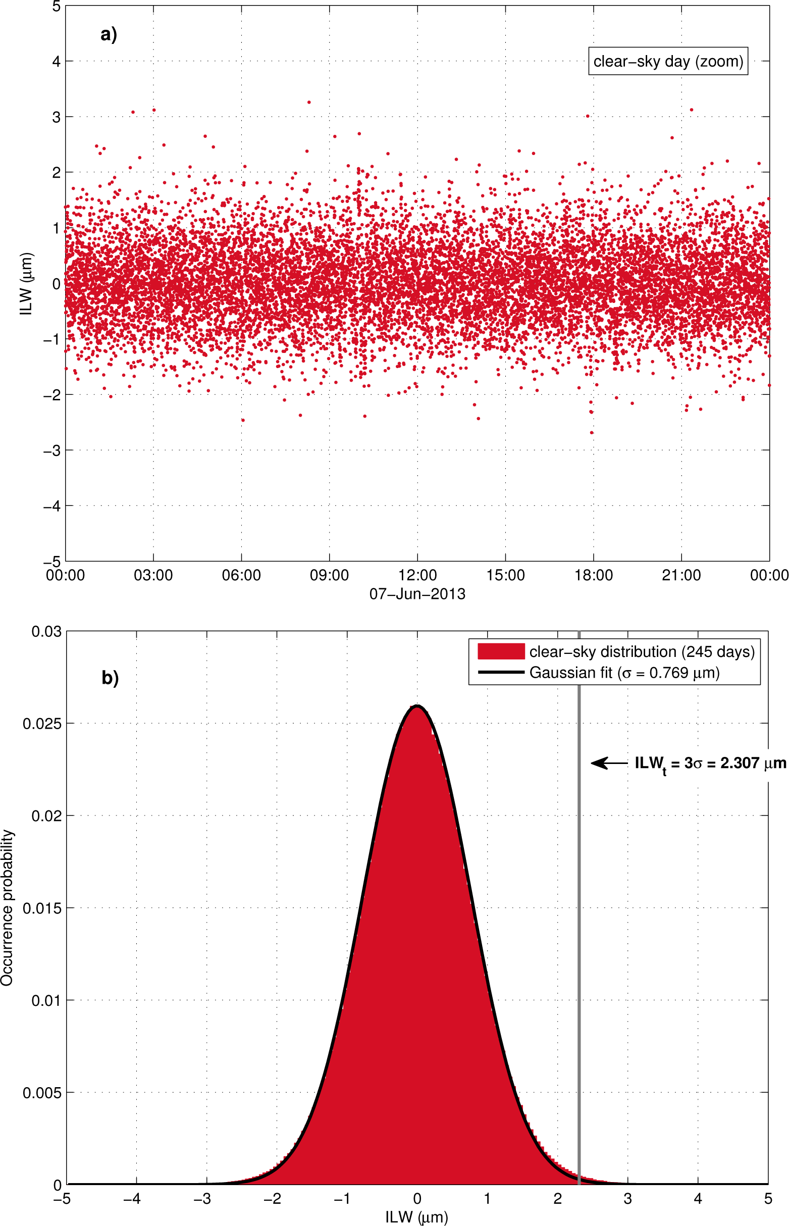
2.2. Cloudy-Sky Threshold

Figure 1 shows an example of TROWARA’s measurements in 3 different situations: Figure 1a, a clear-sky day; Figure 1b, a day with cloudy sky, but without rain; and Figure 1c, a day with rain. On a clear-sky day, ILW oscillates around zero, and it usually does not exceed 5 μm (Figure 2a, where 1 μm = 10⁻³ mm = 10⁻³ kg· m⁻²). On a cloudy day, TROWARA measures positive ILW values with enough resolution to detect variations that occur within one minute. A rainy day is easily recognizable by the continuous values at 0.4 mm (the maximum value allowed for ILW in our retrieval algorithm) during rain, when the emission from rain droplets is much higher than the emission from cloud droplets. Frozen precipitation, such as snow, hail or graupel, does not affect ILW measured by TROWARA, because, due to the small dielectric loss of ice, the absorption of such frozen hydrometeors can be ignored.

Figure 1a represents a special case, because at the location of Bern, it is rare to have 24 hours of continuous clear sky, and usually, clear-sky and cloudy-sky conditions alternate on the same day (combination of Figure 1a,b).

Since we are interested in deriving a climatology for CF, defined as the percentage of time in which TROWARA detects clouds over an averaging period of one month, we need to establish a threshold (ILW_t, cloudy-sky threshold) beyond which the ILW values represent cloudy conditions with a certain degree of confidence.

As we have seen in Figure 2a, when there are no clouds, the value of ILW is not exactly zero, but oscillates around zero (instrument random error). We selected from the 10-year time series the days with small ILW absolute values (−5 μm < ILW < 5 μm), corresponding to clear-sky conditions, finding only 245 days out of 3653 days, which confirms the rarity of such conditions. The corresponding distribution (Figure 2b) appears to be Gaussian in shape. In fact, by fitting the distribution with a single-term Gaussian model, we obtain an R-squared value of 0.9998. The standard deviation of the Gaussian model fit gives us the instrument random error for clear-sky conditions, which is σ = 0.769 μm. A typical cloudy-sky situation will have an ILW value greater than σ.

We can now choose ILW_t as a function of σ. By taking ILW_t = 3 σ =2.307 μm, we can say that all of the values above this threshold represent cloudy-sky conditions with a confidence level of 99.9%.

3. Results and Discussion

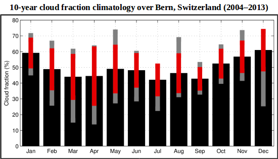
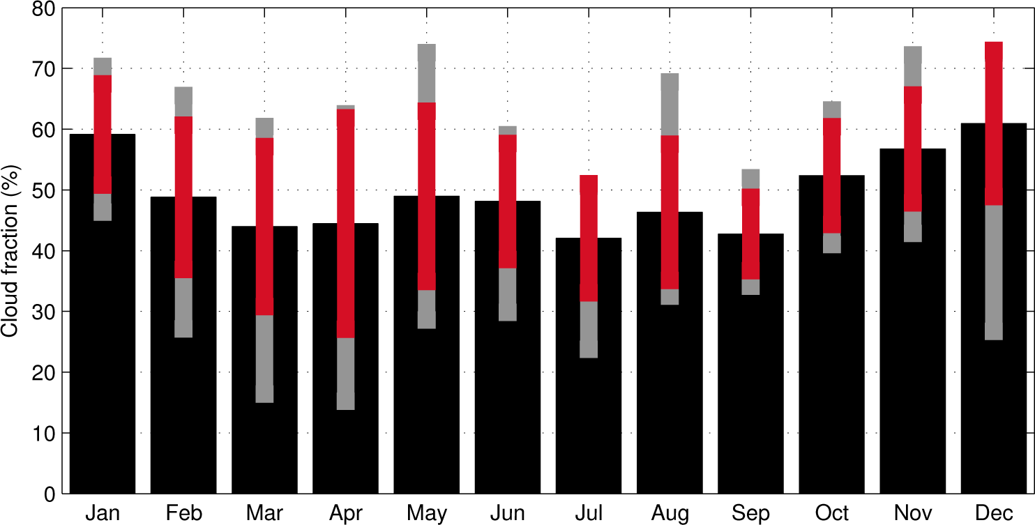
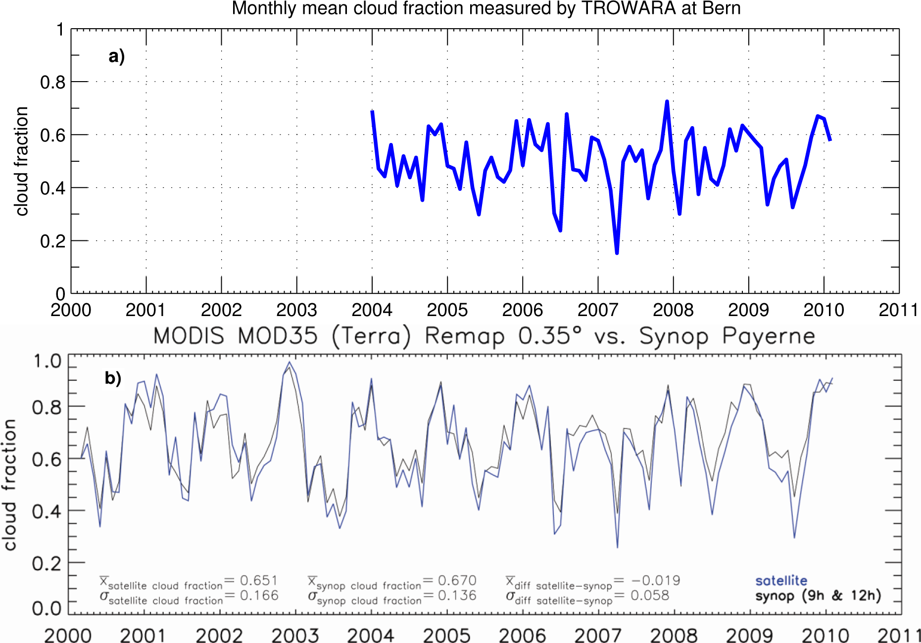
3.1. 10-Year CF Climatology

The 10-year CF climatology over Bern for the period 2004–2013 (

Table 1. Ten-year cloud fraction (CF) climatology over Bern for the period 2004–2013. The columns are, in order: mean CF, CF standard deviation, minimum and maximum CF values for each month.

	Cloud Fraction (%)
	Mean	Std.	Min	Max
January	59.1	8.3	46.3	70.3
February	48.8	11.9	27.1	65.5
March	44.0	13.2	16.4	60.4
April	44.5	17.4	15.2	62.5
May	48.9	14.0	28.6	72.6
June	48.1	9.5	29.9	59.1
July	42.0	9.0	23.8	50.6
August	46.3	11.2	32.5	67.8
September	42.7	6.0	34.2	52.0
October	52.4	8.0	41.0	63.2
November	56.7	8.9	42.8	72.2
December	60.9	12.0	26.7	72.6

and Figure 3) was derived by computing the 10-year average CF for each month. The CF was computed by counting the percentage of measurements with ILW > ILW_t in each period. The most cloudy months occur in fall and winter, and the least cloudy in spring and summer. December has the highest CF (60.9%) and July the lowest (42.0%).

The year-to-year CF variability is different along the season. The red bars in Figure 3 show the CF standard deviation and the grey bars the range between minimum and maximum CF values. April has the greatest variability, with a standard deviation of 17.4%, and September is the most regular month, with a standard deviation of 6.0%.

The 10-year (March 2000–February 2010) monthly mean CF values obtained by Seiz et al. [15] using data from the Moderate Resolution Imaging Spectroradiometer (MODIS) for an area encompassing all of Switzerland are higher than the values of Table 1: 71% for January, 68% for April, 52% for July and 65% for October. The seasonal variation is however in agreement with our results, with the highest CF values in winter and the lowest in summer.

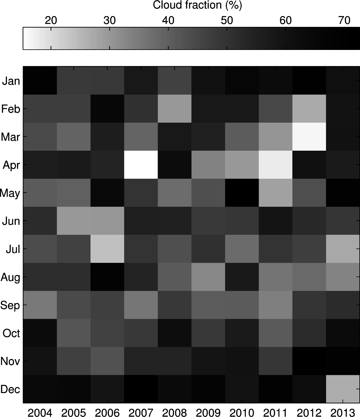
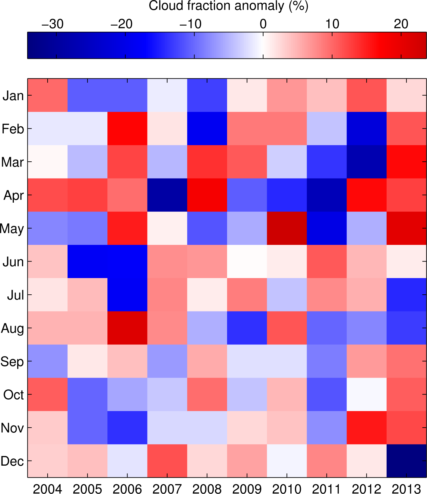
3.2. Monthly Means and Anomalies

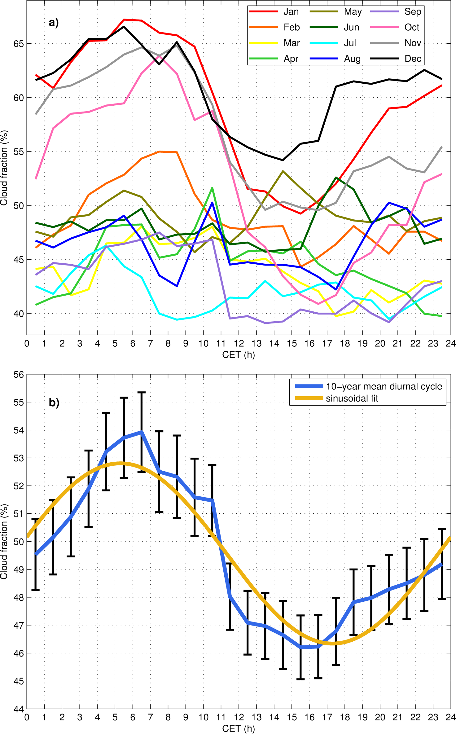
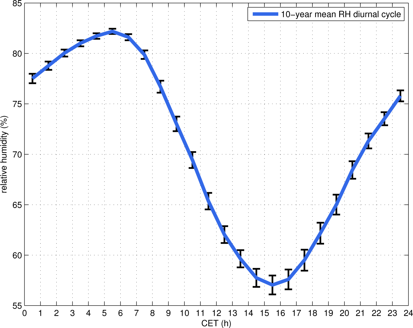
Figure 4 shows CF specifically for each month of every year from 2004 to 2013. In this figure, it is easy to identify the months with the highest and lowest values of CF. Even though July is the month with the lowest CF in the 10-year average (Figure 3), April 2007 is the month with the lowest CF of the whole period with a CF of 15.2%. For the highest CF values, May 2010 and December 2007 are the months with the maximum CF value, having both a CF of 72.6%.

The monthly CF variations measured by TROWARA are in good agreement with the daytime monthly mean CF derived by Seiz et al. [15] using both satellite and ground-based synoptic observations for Payerne, Switzerland (46.80° N, 6.93° E, 490 m a.s.l.). Payerne is located about 42 km southwest of Bern. For satellite observations from the MODIS instrument onboard the Terra satellite [23] (overpass times between 9:00 and 12:00 UTC), Seiz et al. [15] assign a cloud fraction of 100% to the MOD35 classes “cloudy” and “uncertain/probably cloudy” and a cloud fraction of 0% to the MOD35 classes “probably clear” and “confident clear”. The monthly Synop Payerne time series are based on the average of two synoptic observations made at 9 h and at 12 h (close to the Terra overpass time) by a local observer and given in octas (0 octas = clear sky, 8 octas = fully covered sky; 9 = fog, treated as eight octas in this study). We report the CF of Seiz et al. [15] in Figure 5b. The period analyzed by Seiz et al. [15] overlaps with our analysis period from January 2004 to February 2010. To facilitate the comparison, we show in Figure 5a the CF time series measured by TROWARA with the same axes of Figure 5b and without the non-overlapping months. Although the CF of Seiz et al. [15] appears higher compared to ours, there is an extraordinary qualitative agreement between the two sites, considering a geodesic distance between them of about 42 km. Both time series show in fact in-phase seasonality. For example, both series capture the very low CF months of July 2006 and April 2007 and the very high CF month of December 2007. This result suggests that the cloudiness of the two sites depends more on the large-scale circulation rather than on local effects. Both sites are located in the Swiss Plateau, where the main source of clouds is represented by the westerly cyclonic low-pressure systems originating in the North Atlantic. The prevailing wind at both sites blows from southwest and on other occasions from northeast [24], advecting in either case the airmass from one site to the other. This atmospheric flow is almost unaffected by the topography of the region between Payerne and Bern, the terrain being relatively flat compared to the surrounding Jura mountains in the north and Bernese alps in the south, resulting in similar observations at the two sites.

The CF bias between Bern and Payerne is probably due to TROWARA’s inability to detect clouds composed of ice particles, such as cirrus clouds, which causes an underestimation of the total cloud cover. Both ground-based Synop observations and satellite-based observations are instead able to detect ice clouds leading to a higher CF compared to ours.

While Figure 4 is useful for the identification of the months with extreme CF values, it is also important to know how much those values deviate from the climatological mean. Therefore, we computed the monthly anomalies by subtracting the CF climatological mean of Table 1 from the monthly CF values of

Table 2. Cloud fraction (%) measured by TROWARA at Bern for every month of the period 2004–2013.

	2004	2005	2006	2007	2008	2009	2010	2011	2012	2013
January	69.1	48.2	48.4	57.7	46.3	60.5	66.0	63.2	70.3	61.5
February	47.2	47.2	65.5	50.6	30.1	57.7	57.6	44.8	27.1	60.1
March	44.2	39.5	56.3	39.1	57.7	55.0	40.7	30.3	16.4	60.4
April	56.1	57.1	54.1	15.2	62.5	33.6	29.9	17.9	61.0	57.0
May	40.8	39.9	64.0	49.8	37.5	43.3	72.6	28.6	43.6	69.4
June	51.9	29.9	30.3	55.4	55.0	48.1	49.1	59.1	52.8	49.3
July	43.8	46.4	23.8	50.0	43.3	50.6	38.0	49.7	47.2	27.6
August	51.4	51.4	67.8	54.1	41.0	32.5	57.4	36.0	38.1	33.3
September	35.3	44.0	46.8	35.9	48.3	40.6	40.7	34.2	49.4	52.0
October	63.2	42.1	46.4	48.5	62.0	48.4	57.1	41.0	52.0	63.0
November	60.0	46.6	42.8	54.2	54.0	59.1	60.5	49.1	72.2	68.9
December	63.9	65.1	59.0	72.6	63.4	67.0	60.1	69.0	62.3	26.7

. The CF monthly anomalies are shown in Figure 6 and listed in

Table 3. Cloud fraction anomalies (%) computed as the difference between the values of Table 2 and the 10-year average values of Table 1.

	2004	2005	2006	2007	2008	2009	2010	2011	2012	2013
January	10.0	−10.9	−10.7	−1.4	−12.8	1.4	6.8	4.0	11.2	2.4
February	−1.6	−1.6	16.7	1.8	−18.7	8.9	8.8	−4.0	−21.7	11.3
March	0.2	−4.5	12.4	−4.9	13.7	11.1	−3.3	−13.6	−27.6	16.5
April	11.7	12.6	9.7	−29.2	18.1	−10.9	−14.5	−26.5	16.5	12.5
May	−8.2	−9.0	15.1	0.8	−11.4	−5.6	23.7	−20.4	−5.4	20.4
June	3.8	−18.2	−17.8	7.3	6.9	0.0	1.0	11.0	4.7	1.2
July	1.8	4.4	−18.3	8.0	1.3	8.6	−4.1	7.6	5.1	−14.5
August	5.1	5.1	21.5	7.8	−5.3	−13.8	11.1	−10.3	−8.2	−13.0
September	−7.4	1.3	4.1	−6.8	5.6	−2.1	−2.0	−8.6	6.7	9.3
October	10.8	−10.2	−6.0	−3.9	9.7	−4.0	4.7	−11.4	−0.4	10.6
November	3.3	−10.2	−13.9	−2.5	−2.8	2.4	3.8	−7.6	15.5	12.1
December	3.0	4.2	−2.0	11.6	2.5	6.1	−0.8	8.1	1.3	−34.2

. The months with the largest positive anomalies are May 2010 (23.7%), August 2006 (21.5%) and May 2013 (20.4%), while the months with the largest negative anomalies are December 2013 (−34.2%), April 2007 (−29.2%) and March 2012 (−27.6%). The large anomaly of December 2013 is due to the persistence of a high-pressure system with cold and dry air, which has strongly inhibited the formation of low stratus clouds (fog) and ensured a particularly sunny period, not only for Bern, but for many other places in Switzerland. In the region between Basel, Bern, Zurich and St. Gallen, December 2013 had record-breaking sunshine. Sunshine of 80–120 hours was recorded instead of the normal 30–50 hours of sunshine [25].

Besides the single-month CF anomalies, there have been periods of several consecutive months with either a positive or a negative CF anomaly. Two particularly strong consecutive positive anomalous periods occurred from February to May, both in 2006 and in 2013. The cumulative CF anomaly (sum of the single months) of those two periods is 53.9% and 60.7%, respectively. Interestingly, the strongest consecutive negative anomalous period occurred exactly for the same months (February–May) in 2011, with a cumulative CF anomaly of −64.5%. During the same year, another four-month period of consecutive negative anomalies occurred from August to November, making 2011 a very dry and sunny year. At the national level, in 2011, the sunshine recorded by the measurement network of MeteoSwiss was 125% higher than the reference mean 1961–1990. At the MeteoSwiss station “Bern/Zollikofen” in 2011, the sunshine was 133% higher and precipitation 23% lower than the climate normal 1961–1990 [26].

3.3. Diurnal Cycle

The continuous measurements of TROWARA allow the examination of the CF 24 hours a day. It is therefore possible to compute the CF diurnal cycle and examine the differences between the different months of the year. Figure 7a shows the CF diurnal cycle of each month averaged over the 10 years of measurements. The time on the x-axis is expressed in Central European Time (CET = UTC + 1), which corresponds to the local time without applying the daylight saving time difference from March to October. January, October, November and December have a sinusoidal-type diurnal cycle with a higher CF in the morning and a lower CF in the afternoon. The CF is reduced in the afternoon because of the evaporation of the cloud droplets caused by solar heating. January has the highest CF value of about 67% and October has the largest diurnal excursion from about 64% CF between 7 and 8 CET to about 41% CF between 16 and 17 CET. February has also a peak in the morning, but its decrease in the afternoon is less marked. March and April are similar, with a peak between 10 and 11 CET. May and June show a peak in the afternoon, between 14 and 15 CET for May and between 17 and 18 CET for June, probably due to convective activity in the warmest hours of the day. July and August show several highs and lows during the day, while September has a clear transition after 11 CET from CF values around 47% to CF values around 40%.

The seasonality does not seem to be the only driver of the diurnal cycle, since a strong intraseasonal variability is present, as months belonging to the same season do not always show a similar behavior. For example, large differences exist between the consecutive months January/February, June/July and September/October. Cloud formation, transport and evolution depend on multiple processes (local thermodynamic parameters, radiation fluxes, large-scale atmospheric circulation, turbulent fluxes, atmospheric moist convection, etc.), which contribute to the variety of CF diurnal cycles shown in Figure 7a.

However, the differences between the different months can be smoothed out by averaging the 120 months of the period 2004–2013 all together, obtaining the 10-year average diurnal cycle shown in Figure 7b with error bars (the error bars are the standard deviations of the mean for each hour). The resulting diurnal cycle has a clear sinusoidal shape, with more clouds in the morning and less in the afternoon. The maximum value, 53.9%, occurs between 6 and 7 CET and the minimum, 46.2%, between 15 and 16 CET. The diurnal cycle is fitted with a sinusoid, which provides an adequate model of the diurnal variation, and it is almost entirely confined within the error bars. The model of the sinusoid is:

$$\mathrm{CF}(t)=A\cos \left(\frac{2\pi (t-\varphi )}{24}\right)+B$$

(1)

where t is the local time (CET), A = 3.2% is the amplitude, ϕ = 5.3 h the initial phase, B = 49.6% the diurnal mean value and the coefficient of determination is 0.87. The period of the day where the diurnal cycle differs most from the sinusoidal fit is between 11 and 13 CET, when there is a quick transition between high morning values and low afternoon values.

The relative humidity measured by the local meteorological station has a similar 10-year average diurnal cycle, shown in Figure 8. The maximum and minimum CF values are in phase with the maximum and minimum relative humidity values. This similarity is consistent with the fact that clouds are more (less) likely to occur in high (low) relative humidity conditions.

Our yearly-averaged CF diurnal cycle with a maximum in the morning and a minimum in the afternoon is consistent with other mid-latitude locations around the world, for both continental clouds [2] and marine stratocumulus clouds [14,27,28].

4. Conclusions

In this paper, we presented for the first time CF observations relative to liquid clouds for Bern, Switzerland, derived from ILW measured by a ground-based microwave radiometer. The cloudy-sky threshold used to compute the CF was defined with a method based on the shape of the ILW distribution for clear-sky days.

The long and continuous series of ILW measurements allowed us to derive a 10-year CF climatology for the period 2004–2013. The highest CF values are found in winter (December CF = 60.9%), the lowest in summer (July CF = 42.0%) and the yearly average is 49.5%. The months with anomalous CF values (compared to the climatological mean) were identified, and an explanation was provided for some of them with the aid of the climate bulletins of the Swiss Federal Office of Meteorology and Climatology. The monthly CF variations compared well with the variations measured at another location on the Swiss Plateau (Payerne), suggesting that the cloudiness at Bern is largely caused by persistent synoptic-scale conditions, which affect different places on the Swiss Plateau at the same time. Payerne showed however a higher CF compared to Bern, probably due to the absence of ice cloud detection in our measurements.

A CF diurnal cycle was also derived, showing intraseasonal variations, from month to month. The overall mean diurnal cycle (mean of the 120 months of the analyzed period) exhibits the typical sinusoidal shape with high values in the morning and low values in the afternoon, due to the evaporation of the cloud droplets by solar heating in the afternoon hours. The maximum variation of the mean diurnal cycle is about 7.7% with the maximum value between 6 and 7 CET and the minimum between 15 and 16 CET.

A 10-year analysis period is a good starting point for deriving CF statistics for Bern. In future, the analysis period will be extended to encompass the most recent years (2014 and 2015) and the years preceding 2004, to obtain an even more reliable climatology. Of particular interest will be the analysis of the year 2014, the warmest so far in Switzerland (and in the world) since the start of the measurements in 1864, and the summer 2014, relatively cool and with very little sunshine [29].

The usefulness of CF observations is not limited to comparisons among different instruments and locations. CF observations can be also used by modelers to evaluate and improve the parameterizations of the complex cloud physics processes.

References

1. Randall, D.; Coakley, J., Jr.; Lenschow, D.; Fairall, C.; Kropfli, R. Outlook for research on subtropical marine stratification clouds. Bull. Am. Meteorol. Soc. 1984, 65, 1290–1301. [Google Scholar]
2. Dong, X.; Xi, B.; Minnis, P. A climatology of midlatitude continental clouds from the ARM SGP central facility. Part II: Cloud fraction and surface radiative forcing. J. Clim. 2006, 19, 1765–1783. [Google Scholar]
3. Dong, X.; Xi, B.; Crosby, K.; Long, C.N.; Stone, R.S.; Shupe, M.D. A 10 year climatology of Arctic cloud fraction and radiative forcing at Barrow, Alaska. J. Geophys. Res.: Atmos. 2010, 115. [Google Scholar] [CrossRef]
4. Carrasco, E.; Carramiñana, A.; Sánchez, L.; Avila, R.; Cruz-González, I. An estimate of the temporal fraction of cloud cover at San Pedro Mártir Observatory. Mon. Not. R. Astron. Soc. 2012, 420, 1273–1280. [Google Scholar]
5. Lazarus, S.M.; Krueger, S.K.; Mace, G.G. A cloud climatology of the Southern Great Plains ARM CART. J. Clim. 2000, 13, 1762–1775. [Google Scholar]
6. Xi, B.; Dong, X.; Minnis, P.; Khaiyer, M.M. A 10 year climatology of cloud fraction and vertical distribution derived from both surface and GOES observations over the DOE ARM SPG site. J. Geophys. Res.: Atmos. 2010, 115. [Google Scholar] [CrossRef]
7. Qian, Y.; Long, C.N.; Wang, H.; Comstock, J.M.; McFarlane, S.A.; Xie, S. Evaluation of cloud fraction and its radiative effect simulated by IPCC AR4 global models against ARM surface observations. Atmos. Chem. Phys. 2012, 12, 1785–1810. [Google Scholar]
8. Kennedy, A.; Dong, X.; Xi, B. Cloud fraction at the ARM SGP site. Theor. Appl. Climatol. 2014, 115, 91–105. [Google Scholar]
9. Xie, Y.; Liu, Y.; Long, C.N.; Min, Q. Retrievals of cloud fraction and cloud albedo from surface-based shortwave radiation measurements: A comparison of 16 year measurements. J. Geophys. Res.: Atmos. 2014, 119, 8925–8940. [Google Scholar]
10. Wu, W.; Liu, Y.; Jensen, M.P.; Toto, T.; Foster, M.J.; Long, C.N. A comparison of multiscale variations of decade-long cloud fractions from six different platforms over the Southern Great Plains in the United States. J. Geophys. Res.: Atmos. 2014, 119, 3438–3459. [Google Scholar]
11. Zib, B.J.; Dong, X.; Xi, B.; Kennedy, A. Evaluation and intercomparison of cloud fraction and radiative fluxes in recent reanalyses over the Arctic using BSRN surface observations. J. Clim. 2012, 25, 2291–2305. [Google Scholar]
12. Butt, N.; New, M.; Lizcano, G.; Malhi, Y. Spatial patterns and recent trends in cloud fraction and cloud-related diffuse radiation in Amazonia. J. Geophys. Res.: Atmos. 2009, 114. [Google Scholar] [CrossRef]
13. Pfeifroth, U.; Hollmann, R.; Ahrens, B. Cloud cover diurnal cycles in satellite data and regional climate model simulations. Meteorol. Z. 2012, 21, 551–560. [Google Scholar]
14. Min, M.; Zhang, Z. On the influence of cloud fraction diurnal cycle and sub-grid cloud optical thickness variability on all-sky direct aerosol radiative forcing. J. Quant. Spectrosc. Radiat. Transf. 2014, 142, 25–36. [Google Scholar]
15. Seiz, G.; Foppa, N.; Meier, M.; Paul, F. The role of satellite data within GCOS Switzerland. Remote Sens. 2011, 3, 767–780. [Google Scholar]
16. Fontana, F.; Lugrin, D.; Seiz, G.; Meier, M.; Foppa, N. Intercomparison of satellite- and ground-based cloud fraction over Switzerland 2000–2012. Atmos. Res. 2013, 128, 1–12. [Google Scholar]
17. Westwater, E.R.; Crewell, S.; Matzler, C. Surface-based microwave and millimeter wave radiometric remote sensing of the troposphere: A tutorial. IEEE Geosci. Remote Sens. Soc. Newsl. 2005, 134, 16–33. [Google Scholar]
18. Mätzler, C.; Morland, J. Refined physical retrieval of integrated water vapor and cloud liquid for microwave radiometer data. IEEE Trans. Geosci. Remote Sens. 2009, 47, 1585–1594. [Google Scholar]
19. Peter, R.; Kämpfer, N. Radiometric determination of water vapor and liquid water and its validation with other techniques. J. Geophys. Res.: Atmos. 1992, 97, 18173–18183. [Google Scholar]
20. Mätzler, C. Ground-based observations of atmospheric radiation at 5, 10, 21, 35, and 94 GHz. Radio Sci. 1992, 27, 403–415. [Google Scholar]
21. Morland, J. TROWARA—Tropospheric Water Vapour Radiometer. Radiometer Review and New Calibration Model; IAP Research Report 2002–15; Institute of Applied Physics, University of Bern: Bern, Switzerland, 2002. [Google Scholar]
22. Morland, J. TROWARA—Rain Flag Development and Stability of Instrument and Calibration; IAP Research Report 2007-14-MW; Institute of Applied Physics, University of Bern: Bern, Switzerland, 2007. [Google Scholar]
23. King, M.D.; Menzel, W.P.; Kaufman, Y.J.; Tanre, D.; Gao, B.C.; Platnick, S.; Ackerman, S.A.; Remer, L.A.; Pincus, R.; Hubanks, P.A.; et al. Cloud and aerosol properties, precipitable water, and profiles of temperature and humidity from MODIS. IEEE Trans. Geosci. Remote Sens. 2003, 41, 442–458. [Google Scholar]
24. MeteoSwiss—Wind roses. Available online: http://www.meteoswiss.admin.ch/home/climate/past/climate-normals/wind-roses.html accessed on 06 March 2015.
25. MeteoSchweiz—Klimabulletin Jahr 2013. Available online: http://www.meteoschweiz.admin.ch/content/dam/meteoswiss/de/Ungebundene-Seiten/Publikationen/Klimabulletin/doc/publi-klimabulletin-jahr-2013.pdf accessed on 08 March 2015.
26. MeteoSchweiz—Klimabulletin Jahr 2011. Available online: http://www.meteoschweiz.admin.ch/content/dam/meteoswiss/de/Ungebundene-Seiten/Publikationen/Klimabulletin/doc/publi-klimabulletin-jahr-2011.pdf accessed on 08 March 2015.
27. Considine, G.; Curry, J.A.; Wielicki, B. Modeling cloud fraction and horizontal variability in marine boundary layer clouds. J. Geophys. Res.: Atmos. 1997, 102, 13517–13525. [Google Scholar]
28. Snider, J.B.; Hazen, D.A. Surface-based radiometric observations of water vapor and cloud liquid in the temperate zone and in the tropics. Radio Sci. 1998, 33, 421–432. [Google Scholar]
29. MeteoSchweiz—Klimabulletin Jahr 2014. Available online: http://www.meteoswiss.admin.ch/content/dam/meteoswiss/de/Ungebundene-Seiten/Publikationen/Klimabulletin/doc/klimabulletin_jahr_def_d.pdf accessed on 16 March 2015.
Figure 1. Integrated cloud liquid water (ILW) measured by TROWARA at 3 different situations: (a) on a clear-sky day (ILW∼0 mm), (b) on a cloudy day (ILW > 0 mm) and (c) on a day with precipitation events, during which ILW assumes the maximum allowed value of 0.4 mm.
Remotesensing 07 07768f1
Figure 2. (a) ILW measured by TROWARA on a day without clouds. The ILW values are scattered around zero and usually never exceed ±5 μm. (b) Distribution of the ILW values measured by TROWARA in clear-sky conditions (red bars). The sample from which the distribution is computed consists of 245 days in which the sky is free of clouds (−5 μm < ILW < 5 μm), as in (a). The black line is the Gaussian fit of the distribution, which provides the standard deviation of the measurement error around zero (σ = 0.769 μm). The grey vertical line is the cloudy-sky threshold ILWt, which we set equal to 3σ. ILW measurements greater than ILWt will correspond to cloudy-sky conditions with a confidence level of 99.9%.
Remotesensing 07 07768f2
Figure 3. Ten-year cloud fraction (CF) climatology over Bern for the period 2004–2013. The black bars represent the 10-year average CF, the red bars the standard deviation and the grey bars the range between the minimum and maximum values.
Remotesensing 07 07768f3
Figure 4. Cloud fraction measured by TROWARA at Bern for every month of the period 2004–2013.
Remotesensing 07 07768f4
Figure 5. Comparison of monthly mean cloud fraction measured (a) at Bern (46.95° N, 7.44° E) and (b) at Payerne (46.80° N, 6.93° E). (a) Cloud fraction time series measured by TROWARA at Bern, shown only for the overlapping period with Payerne (January 2004–February 2010). (b) Comparison of MODIS Terra (based on MOD35 data, averaged at 0.35°grid) daytime monthly mean cloud fraction product with ground-based Synop observations at Payerne. The monthly Synop Payerne time series are based on synoptic observations made every three hours by a local observer (average of 9 h and 12 h observations). This figure has been taken from Seiz et al. [15] (Figure 3 in their study).
Remotesensing 07 07768f5
Figure 6. Cloud fraction anomalies compared to the 10-year average values of Table 1.
Remotesensing 07 07768f6
Figure 7. Cloud fraction diurnal cycle measured by TROWARA at Bern. The time on the x-axis is in CET (Central European Time). (a) Cloud fraction diurnal cycle for each month averaged over the 2004–2013 period. (b) Blue line: 10-year mean cloud fraction diurnal cycle (averaged over 120 months) with the black bars showing the standard deviation of the mean for each hour. Yellow line: sinusoidal fit.
Remotesensing 07 07768f7
Figure 8. Relative humidity diurnal cycle measured by the local meteorological station at Bern. The time on the x-axis is in CET (Central European Time). The blue line shows the 10-year mean relative humidity diurnal cycle (averaged over 120 months) with the black bars showing the standard deviation of the mean for each hour. The relative humidity diurnal cycle is in phase with the cloud fraction diurnal cycle (Figure 7).
Remotesensing 07 07768f8