Article

Characterization of Land Transitions Patterns from Multivariate Time Series Using Seasonal Trend Analysis and Principal Component Analysis

by
Benoit Parmentier
1,2,3,4
1
Clark Labs, Clark University, 950 Main Street, Worcester, MA 01610, USA
2
Graduate School of Geography, Clark University, 950 Main Street, Worcester, MA 01610, USA
3
National Center for Ecological Analysis and Synthesis, University of California Santa Barbara, 735 State Street, Suite 300, Santa Barbara, CA 93101, USA
4
Sustainability Solutions Initiative, University of Maine, Deering Hall Room 302, Orono, ME 04469, USA 
Remote Sens. 2014, 6(12), 12639-12665; https://doi.org/10.3390/rs61212639
Submission received: 5 October 2014 / Revised: 5 December 2014 / Accepted: 8 December 2014 / Published: 16 December 2014

Abstract

:
Characterizing biophysical changes in land change areas over large regions with short and noisy multivariate time series and multiple temporal parameters remains a challenging task. Most studies focus on detection rather than the characterization, i.e., the manner by which surface state variables are altered by the process of changes. In this study, a procedure is presented to extract and characterize simultaneous temporal changes in MODIS multivariate times series from three surface state variables the Normalized Difference Vegetation Index (NDVI), land surface temperature (LST) and albedo (ALB). The analysis involves conducting a seasonal trend analysis (STA) to extract three seasonal shape parameters (Amplitude 0, Amplitude 1 and Amplitude 2) and using principal component analysis (PCA) to contrast trends in change and no-change areas. We illustrate the method by characterizing trends in burned and unburned pixels in Alaska over the 2001–2009 time period. Findings show consistent and meaningful extraction of temporal patterns related to fire disturbances. The first principal component (PC1) is characterized by a decrease in mean NDVI (Amplitude 0) with a concurrent increase in albedo (the mean and the annual amplitude) and an increase in LST annual variability (Amplitude 1). These results provide systematic empirical evidence of surface changes associated with one type of land change, fire disturbances, and suggest that STA with PCA may be used to characterize many other types of land transitions over large landscape areas using multivariate Earth observation time series.

Graphical Abstract

1. Introduction

Characterizing change over large areas remains an important challenge in remote sensing and land change science [1,2,3,4]. In particular, remotely-sensed time series are often short and noisy, necessitating heavy pre-processing and sophisticated methodology to extract useful temporal patterns [5,6,7,8,9,10]. This research seeks to advance land cover change monitoring by presenting a method that combines seasonal trend analysis (STA [11]) and principal components analysis (PCA) to characterize temporal patterns in land change areas from multivariate image time series. We illustrate the procedure by characterizing biophysical trends in Alaska using burned areas as an example of change with three surface state variables: Normalized Difference Vegetation Index (NDVI), land surface temperature (LST) and albedo (ALB).
Despite multiple research efforts under way, there is a need to improve existing methods to characterize land cover change over large areas [4,12,13,14,15] by exploiting temporal patterns from time series. Most studies have focused on the detection of land cover change [16,17,18] or the filling of missing observation [7,8], rather than the characterization of change, i.e., the manner by which surface characteristics (e.g., attributes) are altered by the process of change [19]. Much information is lost in describing change into change/no-change Boolean categories. Land cover types are characterized by a set of biophysical properties related to their structure and constitutive materials [19,20,21]. These properties regulate land surface atmosphere exchanges and affect the local climate, as well as fluxes in water, carbon and energy [20,22]. Consequently, when land transitions (i.e., modifications or changes in attributes) occur, land-atmosphere fluxes are impacted, and biogeophysical feedback mechanisms may enhance or suppress exchanges at local, regional or global scales [20]. In particular, a browning or greening in forest cover, as described by decrease/increase in NDVI, can impact skin temperature and surface albedo. Experiments using regional and global circulation models illustrate that afforestation in high latitudes would result in increased radiative forcing acting as a positive feedback due to a decrease in albedo [23,24]. More generally, land surfaces are characterized by roughness, sensible heat, latent heat and albedo values that depend on the structure and the nature of land cover types [20]. Thus, land transitions affect multiple surface properties simultaneously, which are part of the biophysical consequences of the land cover change process [25,26]. Documenting and tracking such characteristic changes may help to infer the land change processes at work and benefits a host of studies [27,28,29] engaged in understanding environmental changes in the Arctic. Furthermore, many studies characterize land cover change by using a single unique times series or by producing some typology or classification rather than providing a concise biophysical representation of change [30]. For instance, Kennedy et al. [31] used temporal patterns to map forest disturbance in the Oregon Northwest Forest using a dense temporal stack of SWIR (short wave infrared) Landsat images to characterize and label change processes into various categories: disturbance, revegetation, disturbance and revegetation. Kulik, Hornsby and Bishop [2] proposed a more complex and generalized typology to monitor and characterize land cover change in forested areas by defining twenty-five transition types. With the growth in the number of variables and parameters used in characterizing land cover change, there is a rapid increase in the complexity of possible relationships and combinations of transitions categories. For instance, Parmentier and Eastman [5], found that a large section of Alaska is detected as changing and summarized change in the seasonal trend by using a simple aggregation rule, such as overlay. Using such method, the authors found that many areas have three changing STA parameters, but were unable to understand and identify the most common combinations of variables present within the detected change areas. As a consequence, in this study, we focus on a priori area of change (burned area) and develop a methodology to characterize the combination of the most important surface changes occurring in change areas.
In this research, we adopt a continuous view of land cover change and use the term land transition to convey continuous modifications in surface conditions/characteristic as related to the process of change, rather than a discrete transition from one land cover class to another (Lambin [21]). Following the literature, this research leverages the temporal content in multivariate image times series by exploiting modifications in seasonal patterns to describe and document land cover changes. Seasonality is useful to track changes in the Earth system [32,33], because different land covers and surfaces present contrasting annual temporal patterns, depending on their characteristics [34,35]. An NDVI time series, for instance, exhibits seasonal curves that show the growth, maturity and senescence of vegetation in annual windows, matching roughly a bell shape in regions with a strong seasonal signal from temperature and precipitation. Typically, the detection of seasonal changes is carried out by fitting parameters of phenological models and by studying the shape parameters over several years using temporal trends analysis [11]. de Beurs and Henebry [6] utilized a quadratic model to describe the annual seasonal curve and the seasonal Mann–Kendall (MK) procedure to study trends in transects located in the high northern latitudes. This research utilizes seasonal trend analysis [11], which is a two-step method that uses the windowed Fourier transform (WFT) or harmonic regression [34,35] with the Theil Sen slope estimator [36,37]. The term WFT will be used to designate both harmonic regressions and Fourier analysis in a time window. Trends in the seasonal NDVI curves are described using the Theil Sen slope estimator, and land cover changes are characterized by examining the temporal patterns [38]. Eastman et al. [39] used STA and the MK to map seasonal trends over the globe using the Global Inventory Modeling and Mapping Studies (GIMMs) NDVI dataset. They used classification to summarize the information from STA. In this study, we consider the different problem of examining and characterizing multivariate seasonal changes related to transitions from unburned to burned categories using the STA method in conjunction with principal component analysis (PCA). This procedure provides a means to characterize and empirically synthetize trends in change “burned” areas in Alaska using multivariate time series of biophysical variables.
We used the case of Alaska and fire disturbance, because multiple studies have shown the importance of fire on the global carbon cycle and the surface energy balance [40,41]. Fire affects the species composition, stand age [42] and landscape configuration [43], as well as surface biophysical processes [20,44]. Although biophysical changes occurring in burned areas have been documented in the scientific literature, most studies have been carried out using either a single variable, such as NDVI [45], albedo [46] or soil moisture [47,48], or by focusing on one or a few individual burn scars [40,41]. To date, biophysical changes have not been documented and studied using these three surface state variables (NDVI-LST-ALB) simultaneously at the landscape level over many burn scars.Given that burning in the boreal forest is forecasted to increase under future climate change scenarios linked to climate variability and pest infestation [49], there is a need to improve our understanding and tracking of burn scars’ impact on the environment, in particular the biophysical changes occurring in burned areas [24].
In this research, LST and albedo are used with NDVI to improve biophysical characterization of land transitions. LST and albedo are key surface state variables that are intricately related to land transitions. Chapin et al. [25,50] demonstrated how land surface temperature and albedo in Arctic Alaska provided a clear signal of surface energy exchanges related to Arctic warming and shrub expansion in the region. In the past, several authors used LST and NDVI variables in unison to study land cover types and land transitions in a variety of environment and context [25,51,52,53]. Lambin and Ehrlich [51] utilized NDVI and LST image time series from the AVHRR sensor to categorize land cover change processes over Sub-Saharan Africa during 1982–1991. Julien and Sobrino [53] used metrics derived from the LST-NDVI regression line (slope, range, regression coefficient) to monitor land cover changes and vegetation dynamics around the world over the 2000–2006 time period. Findings indicated that biomes, such as temperate forest, tundra and boreal forest, are clearly separable, because they have different LST-NDVI relationships [53]. Similarly, Kaufman et al. [54] investigated the linear relationship between surface temperature and NDVI for different land cover categories in North America and Eurasia. The authors found that higher NDVI was related to lower surface temperature during summer, but with higher temperature in winter. They attributed these differences to albedo feedback effects and evapotranspiration [25,44,55]. Nemani and Running [52] proposed a biophysical interpretation of the LST-NDVI relationship based on land surface processes in the North American continent. They identified a disturbance trajectory in the LST-NDVI feature space and distinguished four groups of land cover corresponding to different biophysical environments: water limited, energy limited, atmospherically decoupled and atmospheric coupled. Relying on Nemani and Runing’s [52] biophysical interpretation, Mildrexler et al. [13] defined a detection index, the “disturbance index” (DI), based on the ratio of annual maximum values of LST and EVI over the ratio of the multiyear mean of LST and EVI. Coops, Wulder and Iwanicka [15] applied the DI to detect disturbances over the North American continent. The research was able to detect a variety of land transitions related to various causes, such as fire (burn scars) and humans (agricultural intensification).
Thus, the goal of this paper is two-fold:
(1)
Most of the focus of previous studies has been on land cover change detection. Characterization of changes using multivariate surface state variables poses an acute problem. In particular, the complexity of relationships and the numbers of combinations of parameters increase rapidly as more variables and land cover types are added, making it challenging to extract the most important temporal patterns describing particular land change processes. The focus of this study is therefore on the development of a general method for temporal characterization of changes using burned areas as an example rather than the mapping or detection of burned areas. We use extensive ancillary information related to fire and its severity to evaluate if trends are meaningful in the context of fire disturbances and the literature. More specifically, there are two research questions investigated: (1) What combination of trends in surface variables characterize change areas that transitioned from the unburned to burned category? (2) How do combined patterns in NDVI, LST and ALB relate to ancillary information, such as land cover and the continuous variable of change-fire severity?
(2)
While the past research suggests that changes in NDVI-LST-ALB are intricately related by surface processes [20,52], to date, there are few studies that provide evidence of simultaneous changes in biophysical measurements at a landscape level, even though the literature has reported on biophysical changes locally at the individual fire area level [41] or regionally with a single variable [40,56]. This research overcomes this challenge by extracting the most common combination of biophysical changes occurring in burned areas with STA and PCA using times series over the 2001–2009 period in Alaska. The principal components extracted provide an empirical summary of characteristic changes in terms of seasonal trends for the three surface states variables. More broadly, our aim is to document and characterize biophysical changes occurring over the landscape level for the benefit of studies [27,28] engaged in understanding environmental changes in the Arctic system.

2. Materials and Methods
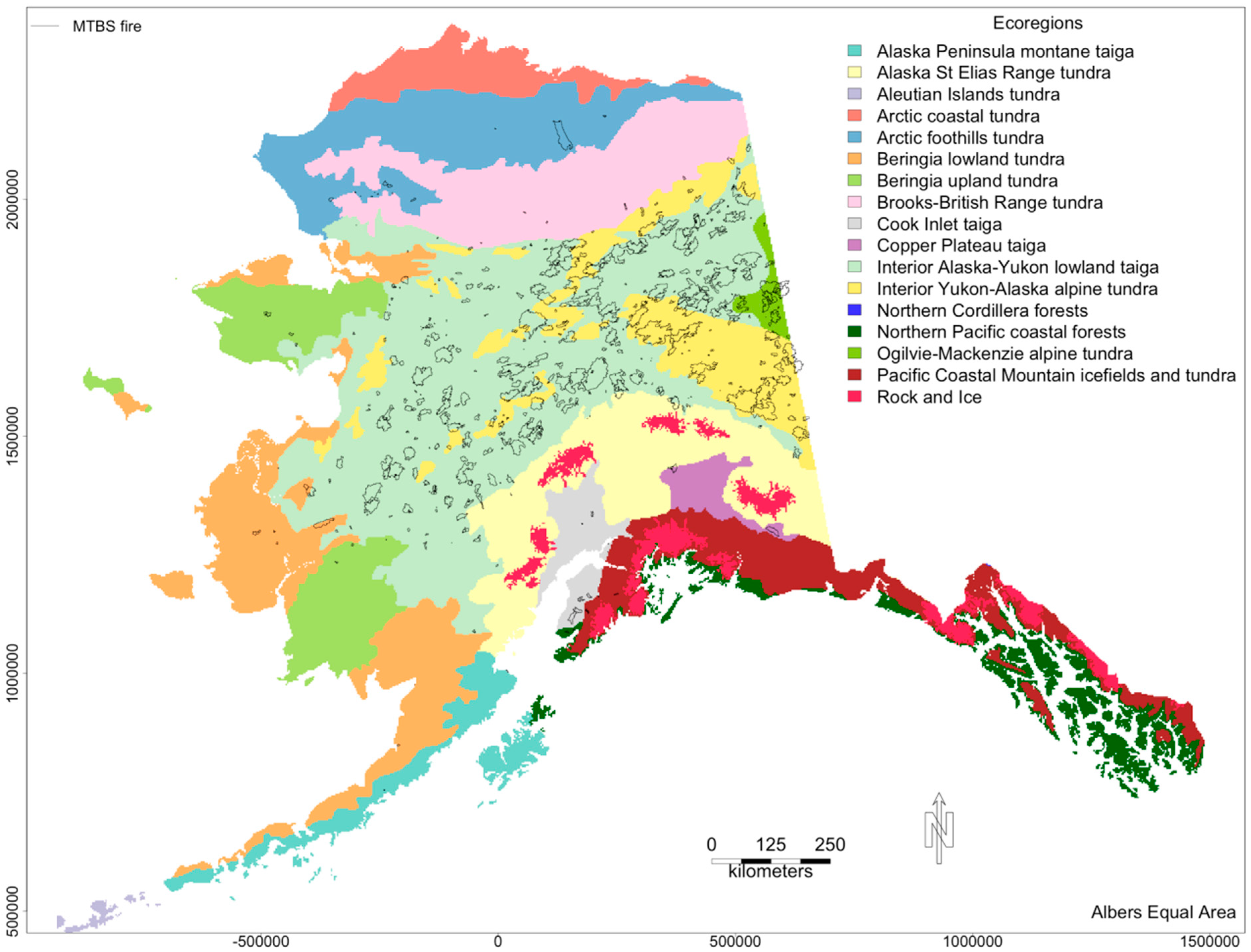
2.1. Study Area

Alaska (Figure 1) has a land mass of about 1.5 million km2 and lies mostly in the Arctic region. The area is undergoing rapid environmental changes with regional warming trends of 1.3 °C/year, surpassing the global trend [25,57,58]. Recorded changes include: (1) changes in plant phenology, such as lengthening of the growing season and changes in plant productivity [27,59]; (2) permafrost thawing [60,61]; (3) wetland losses [62]; (4) increases in disturbance regimes, such as fire and insects [63,64,65,66]; and (5) shrub expansion in tundra [67]. Alaska has a complex landscape with 17 ecoregions (Figure 1), a varied topography composed of many mountains (e.g., the Brooks Range), coastal plains (e.g., the North Slope) and large river basins (e.g., the Yukon and Tanana).
Wildfire and insect outbreaks constitute the main drivers of land change in the State of Alaska [63,68]. The fire season typically starts in May and ends in September, with most fires occurring in the middle and end of the season when the ground cover is free from snow and the soil is drier. The fire regime is characterized by an annual average of 767,000 ha (the 2000’s decadal average) and a return interval of 105 years for the 1920–2009 period [65]. Analysis of the 2000’s fire regime data showed that 95.5% (43/45) of fires greater than 50,000 ha were wildfires caused by lightning. Nevertheless, human ignited fires are expected to rise as population increases [65]. Changes in the fire regime associated with climate change may affect the carbon balance [49,66,69], as well as surface processes, in particular albedo and surface temperatures [20,40]. Increases in fire frequency and severity are likely to lead to an increase in the proportion of boreal deciduous tree cover [56,70], which, in turn, will result in an increase in albedo, causing a negative feedback for warming [41].
Studies demonstrate that Alaska impacts the global carbon budget and acts currently as a net carbon sink [49]. There are concerns, however, that the region may become a carbon source in the future as temperatures increase and climate change occurs [66,71]. Projections using dynamic climate models indicate that under future climate change scenarios, burned areas will increase from 360,000 ha per year to 411,000–481,000 ha for the 2025–2099 time period [71]. Fire emissions are expected to increase by 24%–33% compared to historical conditions, reaching an average release of 17–19 Tg∙Cy−1 from 2025–2099 [71].
Figure 1. Study area with 17 ecoregions (World Wildlife Fund biome classification, Olson et al. [72]) and fire polygons.
Remotesensing 06 12639 g001

2.2. Data Source

This research utilizes three time series from the MODIS sensor (Table 1): NDVI (MODIS13A2, [73]), LST (MOD11A2, [74]) and albedo (MCD43B3, [75]). All products have a 1-km resolution and span the 2001–2009 time period. MODIS version 5 products were downloaded from the Land Processes Distributed Active Archive Center [76], and tiles were mosaicked and reprojected to the Albers equal area projection using the North American Datum 83 (NAD83) datum.
Table 1. Datasets include three biophysical variable products, two ancillary datasets related to fire and one albedo quality product. MTBS, Monitoring Trends in Burn Severity; NLCD, National Land Cover Database; dNBR, difference normalized burn ratio; LST, land surface temperature; ALB, albedo.
Product Platform Variables Code NameSpatial Resolution Temporal Resolution
MOD11A2TerraLand Surface Temperature LST1000 m8 Day
MOD13A2TerraVegetation IndexNDVI1000 m16 Day
MCD43B3 CombinedAlbedo ALB1000 m16 Day
MCD43B2CombinedAlbedo qualityALBQ1000 m16 Day
MTBSLandsatFire Severity Index (dNBR)dNBR30 mAnnual
MTBS NA Burned areas-Fire perimeters BURNEDNA annual
MTBSNAIgnition date, Fire sizeSeverityNAAnnual
NLCDLandsatLand coverLC30 mNA
The quality information was used to remove pixels with cloud contamination and of low quality, as defined by the flag layers in the LST, NDVI and ALB (MC43B2) products. Gap-filling procedures were applied to reduce the amount of missing data by using linear temporal interpolation and climatology-based filling procedures. Linear temporal interpolation fills pixel values based on values surrounding gaps, while climatology procedure fills missing data by computing median values for the relevant time period (see Eastman [38] for details). Since LST and ALB are distributed as 8-day products, both datasets were aggregated to a 16-day time period to match the NDVI product.
Three ancillary/validation datasets were used in this research: fire perimeters, fire severity and land cover data (Table 1). The fire perimeters and severity information originate from the Monitoring Trends in Burn Severity (MTBS) database [77]. MTBS contains information on ignition dates, ignition sources, as well as management information from the 1984 to 2011 time period. In this study, fire severity is used as a continuous validation variable of change to interpret and evaluate temporal trends. Fire severity is measured via the difference normalized burn ratio (dNBR) index, which is generated by the difference between the normalized burn ratio (NBR). NBR is derived from the NIR and red Landsat bands. The dNBR product was aggregated from the 30-m Landsat resolution to the 1-km MODIS spatial resolution using mean averaging. Since the dNBR index is known to be a problematic measure of severity, because it shows low correlation in small fire areas and is influenced by environmental conditions [78], the MTBS fire perimeter database was also used to produce a Boolean severity index using and combination of the date of ignition and size of fire, following Beck et al. [56], approach. In addition, the size of fire was also used to interpret results in terms of severity.
The third ancillary dataset consists of the National Land Cover Database (NLCD) developed using Landsat imagery [79]. This dataset has 30-m resolution and pertains to the year 2001, therefore allowing the categorization of land cover at the beginning of the time series. Land cover types were recorded in 6 fuel types following Kasischke and Hoy [80]: Non-woody vegetation (NWV), low shrub (LSH), high shrub (HSH), deciduous forest (DEC), mixed forest (MX) and evergreen forest (EGF). The proportion of evergreen in every burned area and the land cover types were both used to interpret the results from PCA.

2.3. Methods

This research utilizes two techniques in conjunction, the seasonal trends analysis (STA) and the principal component analysis (PCA), with the aim of characterizing surface temporal trends related to land change areas caused by fire disturbances. The method proceeds in three stages: (1) STA is applied to extract amplitudes (Table 2) and produce Theil Sen slope images; (2) a change/no-change area mask is produced from the MTBS database; and (3) PCA is carried out on slope images in the masked areas to characterize change (Figure 2a).
Stage 1: Seasonal Trend Analysis
Stage 1 applies STA to each data series [11]. This is a two-step process that consists of applying a Windowed Fourier Transform (WFT) to extract seasonal shape parameters and of using the Theil Sen slope estimator to generate seasonal trends. Eastman et al. [11] found that the information contained in Frequency 1 (annual seasonality) and Frequency 2 (semi-annual pattern) is sufficient to describe a wide range of seasonal changes related to many types of land cover change. Thus, only these two frequencies are utilized in the study. Exploratory tests showed that Fourier phases were affected by noise, so that the final set of parameters was reduced to three amplitudes: Amplitude 0, Amplitude 1 and Amplitude 2. In total, there are nine times series of amplitudes for the three original time series, adding up to 81 images.
The second step consists of calculating temporal trends using the Theil Sen (TS) slope procedure [81], which is a non-parametric estimator based on the median values of pairwise combinations [36,37]. In contrast to ordinary least squares (OLS) estimates, which are strongly affected by outliers, Theil Sen estimates are robust against outliers and have a breakdown bound of 29% [82]. In the current context, this means that estimates for pixel locations containing two outliers or less are not affected. For every shape parameter, a slope was estimated using the Theil Sen (TS) operator producing nine TS slope images, which served as input in the PCA and the segment-based detection of trends and change (SDTC) method [5].
Stage 2: Change-no change mask: Burned-Unburned areas
Stage 2 consists of defining the change and no-change locations using the MTBS Database (MTBS 2011). Burned areas corresponding to the 2001–2009 period are selected from the database, and for each burn scar, an equal number of unburned pixels are selected in the direct vicinity. Unburned pixels for each fire scar were selected using the following procedure:
  • Delineate an area of selection for potential unburned candidate pixels for each scar.
  • Allocate unburned candidate pixels to the closest fire scar and limit pixels to a threshold distance (20 km in this study).
  • Randomly select pixels within the zone of selection.
The procedure was programmed as a Python script using the IDRISI API. A subset (mask) was created with 146,426 pixels, from which 49.8% were unburned (72,861) and 51.2% were burned (73,565). Since the research focuses on the characterization of surface change, the approach used the whole fire dataset and did not set aside data for validation. Unburned pixels act as the reference no-change category to which trends in the change category (burned pixels) are compared.
Stage 3: Principal Component Analysis to characterize surface trends
Stage 3 consists of applying a standardized PCA on the nine TS slope images in the mask comprising burned and unburned areas. PCA produces new composite variables, principal components, which are based on the combination of the input STA parameters and concentrate the information into independent portions of variability [83]. PCA allows extracting empirically simultaneous combinations of NDVI-LST-ALB trends in the burned area. Thus, PCA allows the characterization of biophysical trends by concentrating the information in a few dominant modes of variability that can easily be used to summarize multivariate trend patterns in change areas.
Figure 2. General analysis workflow. (a) PCA-STA method: (1) STA is applied using a Windowed Fourier Transform and the Theil Sen estimator to produce slope images; (2) a mask for burned-unburned area is produced; (3) a PCA is performed on the TS slope images. (b) Evaluation: the shape parameters are combined and analyzed together using ancillary data (e.g., severity as dNBR) and the SDTC method.
Remotesensing 06 12639 g002
Table 2. Amplitudes obtained from the Windowed Fourier Transform: there are nine shape parameters related to the seasonal curves for the land surface temperature (LST), the Normalized Difference Vegetation Index (NDVI) and the albedo (ALB).
Shape ParameterWindowed Fourier Parameter and Interpretation
NDVI_A0Normalized Difference Vegetation Index Amplitude 0: Annual average relating to biomass
NDVI_A1Normalized Difference Vegetation Index Amplitude 1: Annual amplitude of plant phenology, photosynthetic activity
NDVI_A2Normalized Difference Vegetation Index Amplitude 2, semi-annual amplitude: Modifies the shape of the seasonal curve
LST_A0Land surface temperature: Amplitude 0, annual average
LST_A1Land surface temperature, Amplitude 1, annual amplitude: Related to annual insolation input and land cover
LST_A2Land surface temperature, Amplitude 2, semi-annual amplitude: Modifies the shape of the seasonal curve
ALB_A0Albedo Amplitude 0: Annual average corresponding to the fraction of visible and NIR reflected by the surface
ALB_A1Albedo Amplitude 1: Annual variability corresponding to seasonal variation of surface albedo
ALB_A2Albedo Amplitude 2, semi-annual amplitude: Modifies the shape of the seasonal curve

2.4. Evaluation Analysis

In the second part of the analysis (Figure 2b), we evaluate the STA-PCA results using ancillary information and the segment-based detection of trends and change (SDTC) method [5].

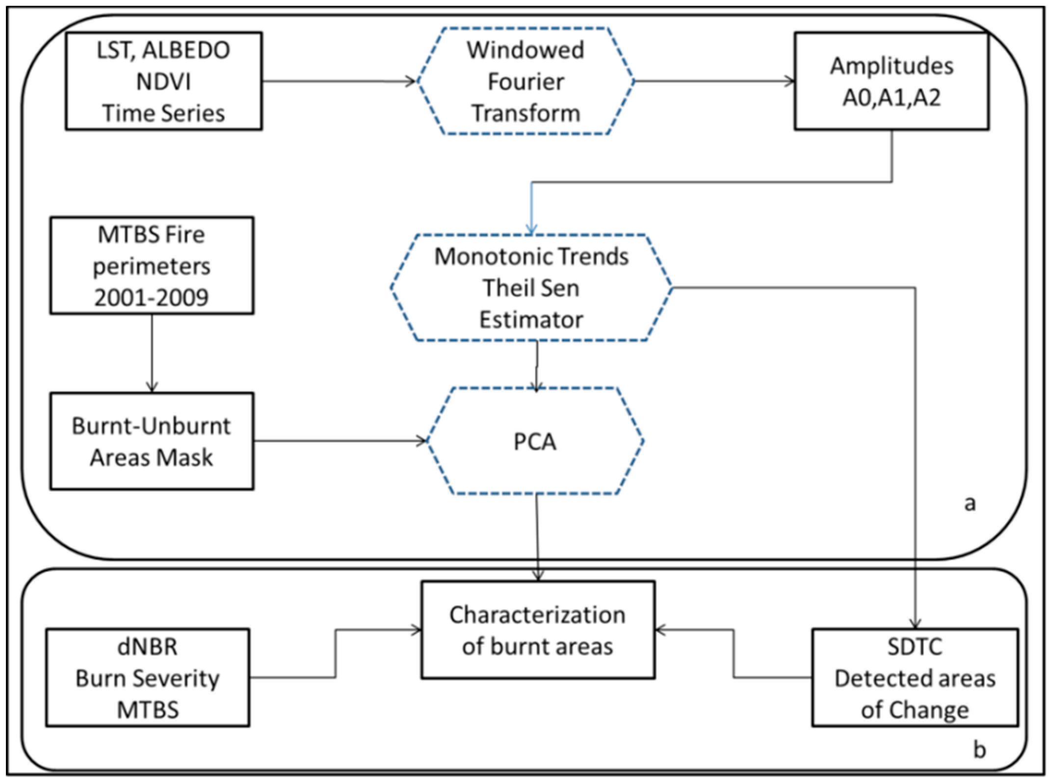
2.4.1. Evaluation-Analysis of Trends Using PCA and Validation Using Ancillary Information

We interpret the PCA components in terms of the combination of seasonal trends and use the ancillary information to evaluate the extraction procedure. The MTBS fire perimeters are utilized to produce a Boolean variable “BURNED” with value “one” corresponding to burned pixels and value “zero” corresponding to unburned pixels. In addition, the dNBR and a Boolean severity index, as well as fire size are also used to evaluate the relationship between PC scores and the continuous validation variable of change: fire severity. Land cover types derived from the NLCD dataset and the proportion of evergreen forest were also used to inform and interpret PC1 scores following the literature [43]. The main goal is to evaluate the change component that shows a combination of the original variables and characterize transitions in change areas. The burned Boolean variable and the burned severity index are utilized as input in a general linear model (henceforth called “LM” to avoid confusion with Generalized Linear Model), with the first principal component (PC1) as the dependent variable. LM is a general regression model that accommodates both continuous and categorical variables. When independent categorical variables are used, it is equivalent to a linear regression with dummy variables and relates to the analysis of variance (ANOVA) [84]. The 2D plot of loadings allows for the visualization of patterns of the relationship between the input Fourier parameters and the principal components. Thus, the 2D loading plot helps in the characterization of biophysical trends in change areas. In addition, the change variable derived from the SDTC method is used to confirm the PCA interpretation. The change variable is plotted along the principal component identified as change, and a LM is performed.

2.4.2. Evaluation-Determination of Number of Changes Using the SDTC Method

We examine how the biophysical changes identified relate to the number of significant changes in STA parameters using the SDTC method [5]. SDTC determines areas of change using segmentation on the nine TS slope images and the Mann–Kendall test. Segments are landscape units corresponding to polygons formed by groups of contiguous pixels with similar TS trend values. There were about 146,000 image segments produced using the watershed-based SEGMENTATION algorithm in IDRISI [38]. The Mann–Kendall procedure was used to flag individual pixel location, and segments were labeled as changing if they included a majority (>50%) of locations with significant Theil Sen slopes. Since there are nine slope images, a segment may contain a maximum of nine changing parameters at once. The change variable was used to record the number of changing parameters for every segment and to interpret the components. SDTC can also be used in the determination of change-no change area if no ancillary information is available.

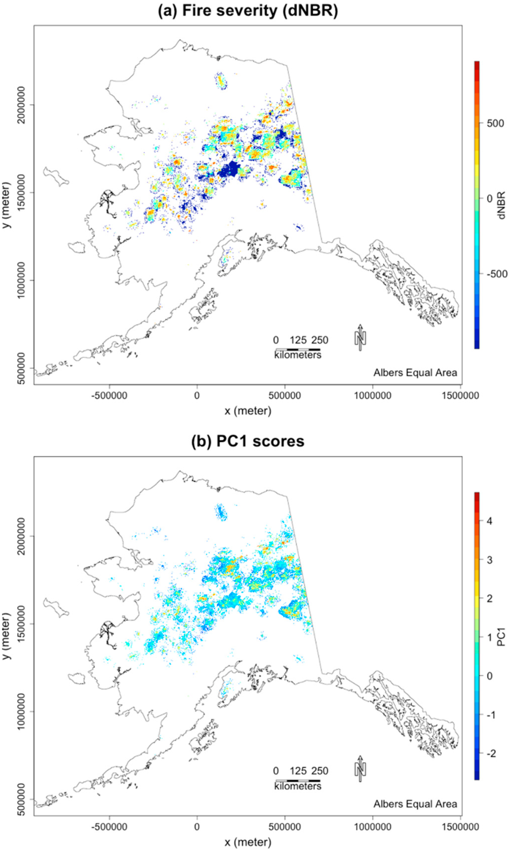
3. Results and Discussions

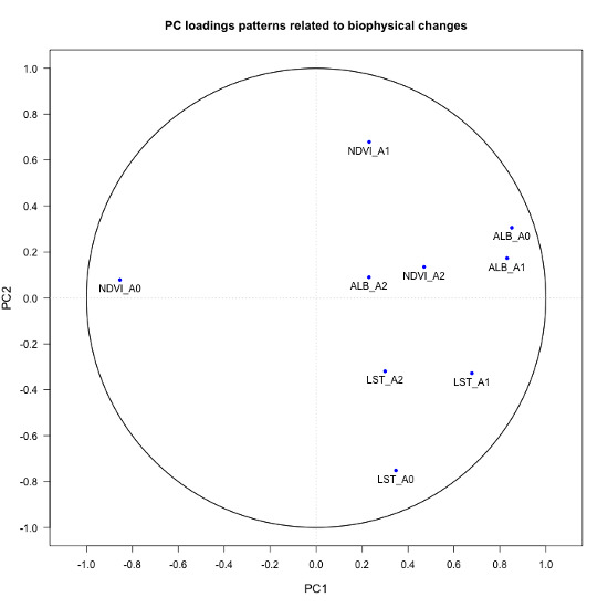
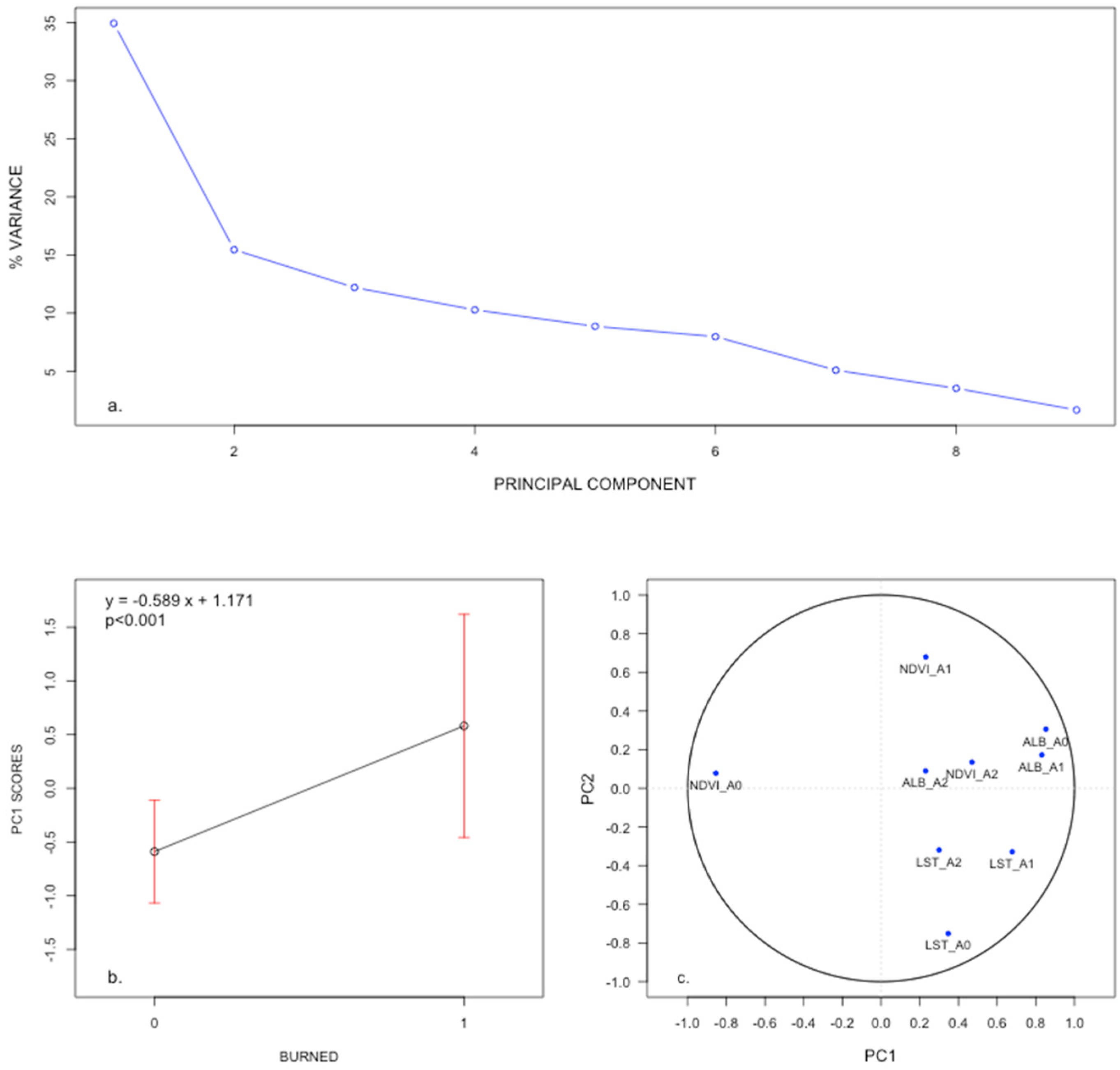
3.1. PCA Results: Variance Explained and Loadings Pattern

PCA results show that the first component (PC1) explains about 35% of the information (Figure 3). Given that a variable would be expected to contribute, on average, to 11.11% (1/9) of the total variance, PC1 stands out in terms of variance explained, as it concentrates an equivalent of 3.14 variables. Only two other components have variances greater than 11.11%: PC2 (15.45%) and PC3 (12.20%). In order to interpret PC1 in terms of land change, the Boolean burned variable “BURNED” is used as the input in an unilabiate normal general linear model (LM1) with the first component as the dependent variable. LM1 is a regression model equivalent to a one-way ANOVA with the BURNED variable corresponding to the factor and the PC1 corresponding to the response variable. LM1 indicates a strong relation between BURNED and PC1 with a Pearson correlation coefficient of 0.586 and a positive slope of 1.171 (with p < 0.001). LM1 also reveals that, on average, unburned pixels have negative scores (−0.589) and burned pixels have positive scores (0.581) (Figure 3b). Thus, LM1 provides evidence that PC1 is a continuous variable change that discriminates between burned and unburned pixels. The loading pattern brings additional information to interpret the trends for positive and negative scores (Figure 3c).
Figure 3. The first component (PC1) is interpreted using: (a) the scree plot showing the % of variance corresponding to each PC; (b) the LM plot illustrating that burned pixels (Category 1) have positive scores and unburned pixels have negative scores (Category 0), (c) the 2D plot of loadings illustrating the strong positive correlation between PC1 and ALB_A0, ALB_A1 and LST_A1, as well as the strong negative correlation between PC1 and NDVI _A0.
Remotesensing 06 12639 g003
Loadings correspond to correlations between the components and the original standardized variables (the nine standardized Fourier TS slopes). The plot of loadings for PC1 and PC2 provides a visualization of the relationships between the components and input trends (Figure 3). The loadings plot indicates that the first component (PC1) displays a strong positive relation with three variables ALB_A0, ALB_A1 and LST_A1 with loading values of 0.852, 0.831 and 0.678, respectively. PC1 also displays a strong negative relation with NDVI_A0 with a loading value of −0.854. This pattern of loadings may be interpreted in the following way: PC1 shows an opposition between positive and negative trends in the two groups of variables. Pixels with high positive scores on PC1 show positive trends in ALB_A0, ALB_A1 and LST_A1 and negative trends in NDVI_A0. Thus, PC1 may be interpreted as a continuous discriminant variable of change for fire disturbance, and burned areas (i.e., pixels with positive scores) show a decrease in average NDVI (NDVI_A0), concurrent with an increase in albedo (both average, ALB_A0, and annual variability, ALB_A1) and in LST annual seasonality (LST_A1). This result indicates that PC1 is able to characterize biophysical changes in burn areas (Research Question 1) based on temporal trends derived from STA.

3.2. PCA Results: Evaluation Using Ancillary/Validation Information Related to Fire

Interpretation of the first component as “land transition” or the change variable suggests differences between burned areas that are strongly affected by fire (high scores) and lightly affected by fire (low scores). Typically, one expects severely-burned pixels to display stronger decreases in average NDVI with concurrent stronger increases in ALB_A0, ALB_A1 and LST_A1. To evaluate temporal patterns, we use validation information, including land cover information and two burn severity indices: dNBR and a Boolean severity index.

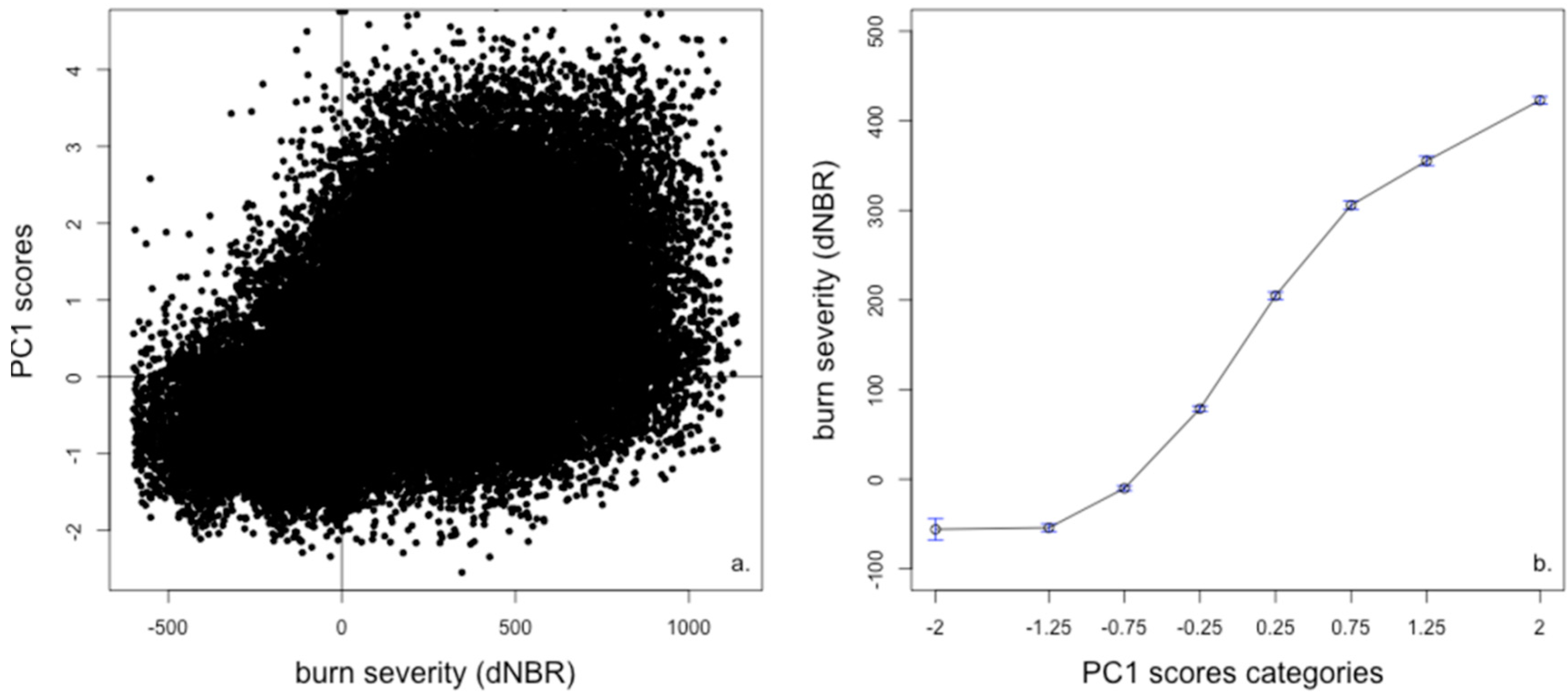
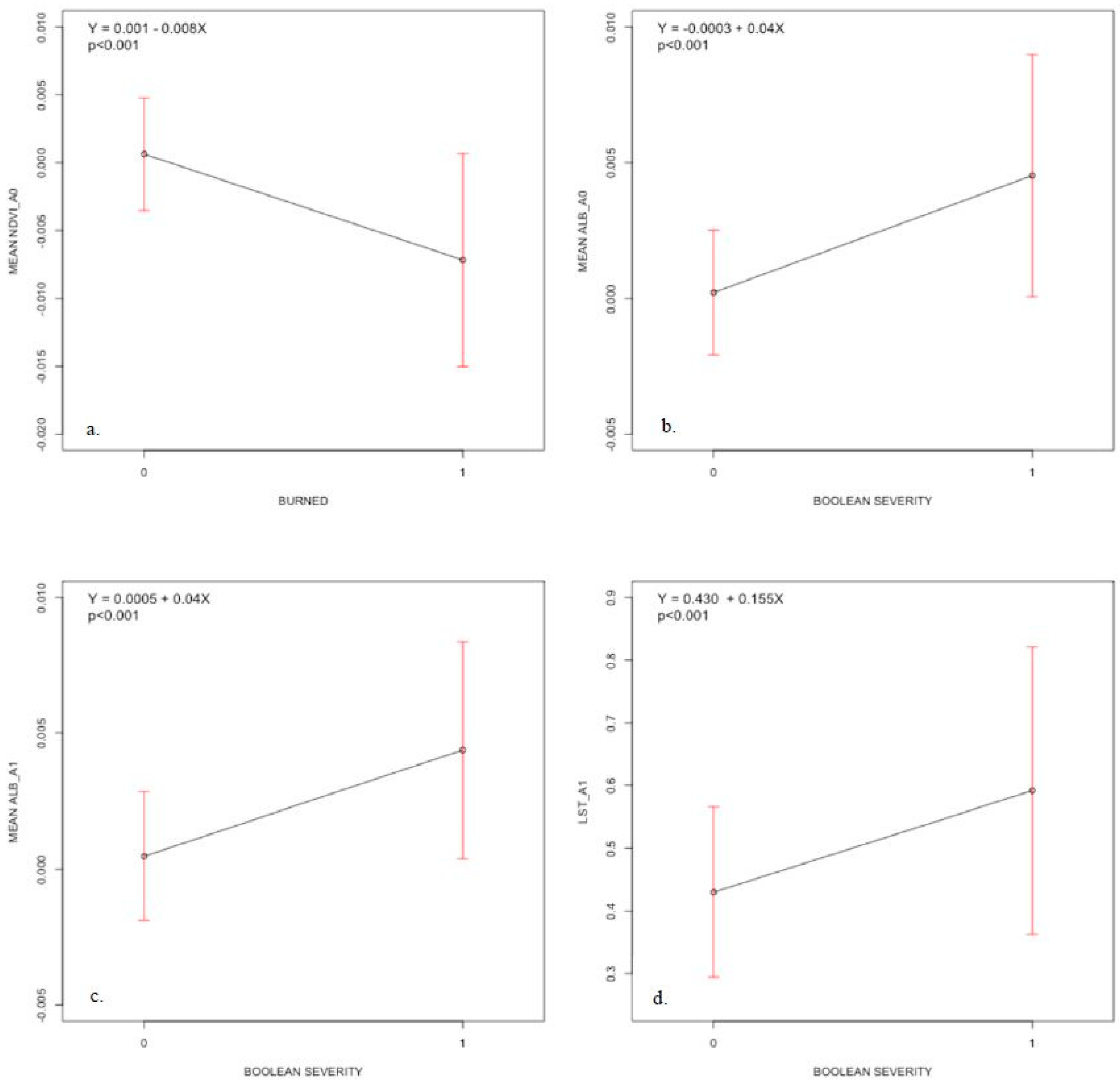
3.2.1. Evaluating PC1 with the Continuous Variable of Change: dNBR Severity

The severity index, dNBR (difference normalized burn ratio), is measured on a continuous scale with a valid range of −600 to 1300 [77]. We used LM1 to relate PC1 scores to the continuous variable of change, dNBR (Figure 4), and we mapped PC1 and dNBR (Figure 5). It was found that dNBR relates to PC1 with a Pearson correlation of 0.5. The scatter plot of values indicates, however, that higher dNBR pixels have higher variance in PC1, i.e., a sign of heteroscedascity that reduces the overall fit (Figure 4a). Burned areas with high positive dNBR values are associated with high PC1 score pixels, while negative values correspond to unburned and/or regrowth areas.
The nature of the relationship between PC1 and dNBR becomes more evident when PC1 is ranked and categorized in eight classes with equal intervals from −2 to 2 for burn scars (Figure 4b). Results conform to our expectation, i.e., mean scores are higher when the severity level increases. Thus, results demonstrate that: (1) pixels with high dNBR values have high scores on PC1, while pixels with low dNBR values have low scores on PC1; and (2) the variance is higher in severely-burned pixels.
Figure 4. Relation between PC1 scores and the continuous variable of change “dNBR”: (a) PC1 scores increase with increasing dNBR, but with higher variance; (b) average dNBR increases for increasing categories of PC1 scores.
Remotesensing 06 12639 g004
Figure 5. Map of the continuous variable of change “dNBR” (a) and PC1 scores (b).
Remotesensing 06 12639 g005

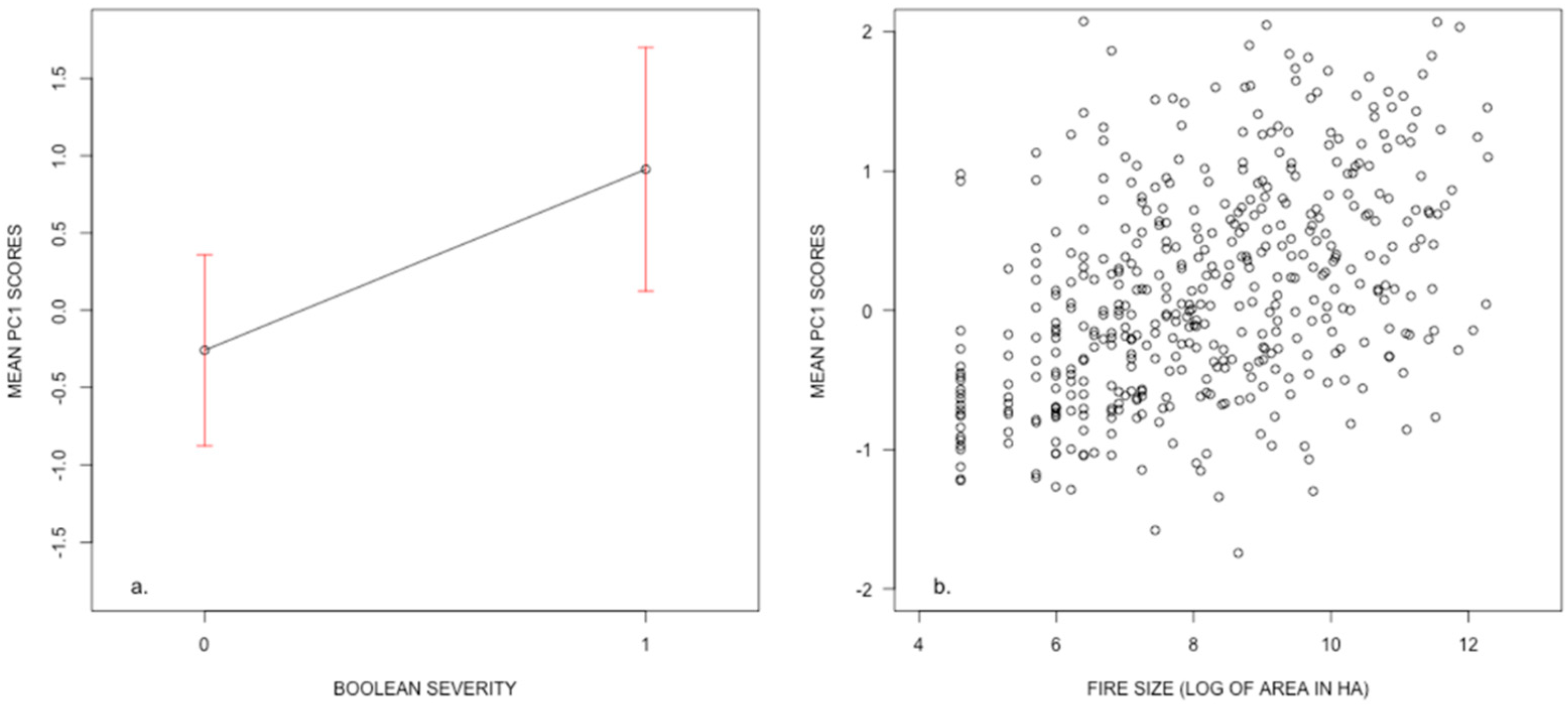
3.2.2. PC1 Scores and Boolean Severity Derived from Fire Size and Date of Ignition

While dNBR is a widely-distributed burn severity index [85] that has been shown to relate to severity of small fire size [43,86], it does not always correlate well with severity observed on the ground (such as the composite burned index, CBI) for large fire areas [87,88]. In order to address this concern and further validate the method, this research derives a Boolean severity index using fire size and date of ignition following the logic described in Beck et al. [56]. Burned areas are coded as high severity (category value = 1) if they have a size greater than 60,000 ha and occurred late in the fire season (after DOY 160, 6 June). The reasoning is that: (1) more severe fires tend to occur later during the summer when the soil is dry and there is more fuel available [89]; and (2) large burned areas are correlated with higher burn severity in the literature [90].
Figure 6. Relationship between PC1 scores and severity: (a) High severity burned areas (Category 1) have a high average PC1 score of about one; (b) the average PC1 score increases with the log of fire size (log(area)).
Remotesensing 06 12639 g006
Results from LM1 indicate that the new Boolean severity index is strongly associated with PC1 scores with a Pearson correlation of r = 0.630 (p < 0.001). High severity burned areas have an average PC1 score of 0.9, while low severity burn scars have mean PC1 scores of −0.3 (Figure 6a). In addition, the relationship between PC1 and fire size also demonstrates that average PC1 scores increase with the log of the fire area (Figure 6b) with a correlation of r = 0.454 (p < 0.001). These results are consistent with findings from the literature, which documents a relationship between burn severity and the logarithm of the burned area [90].

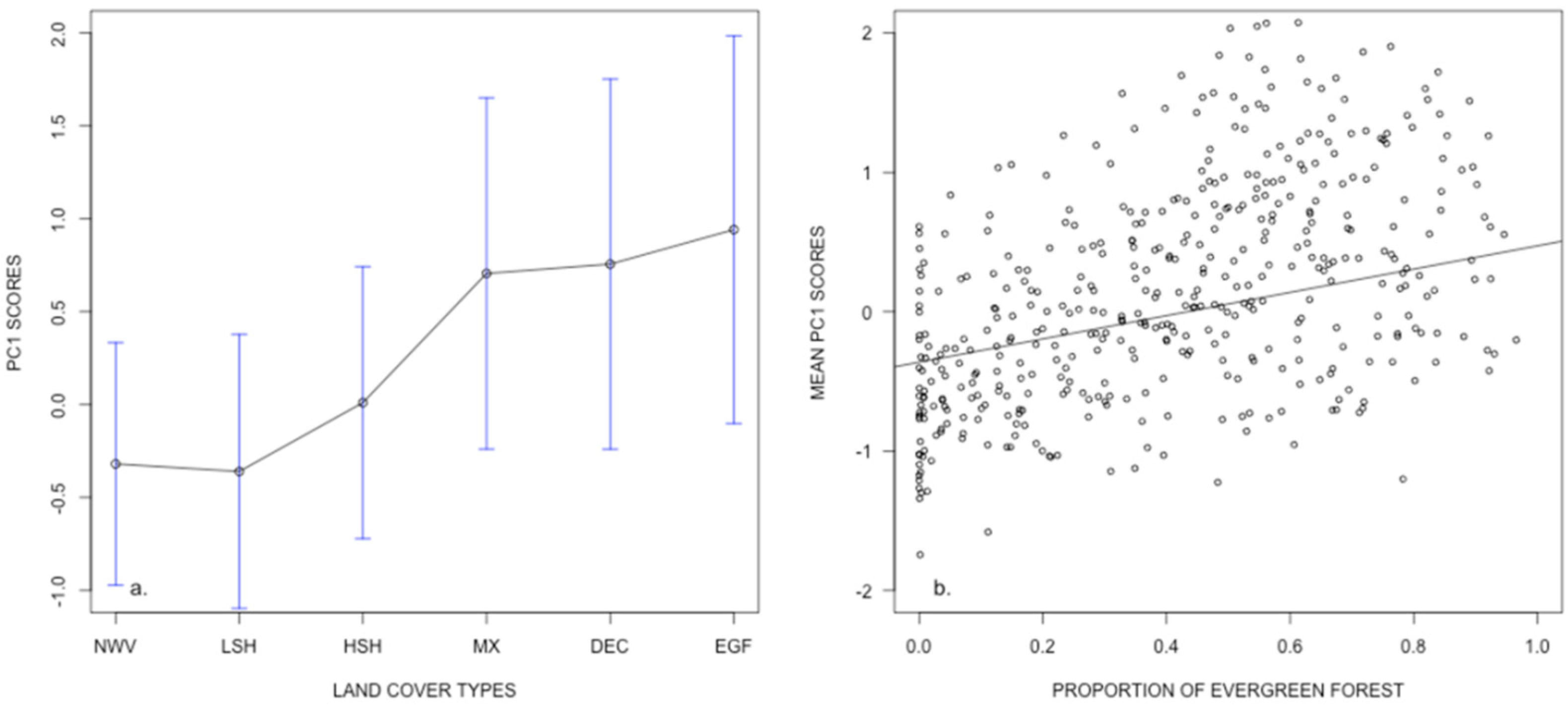
3.2.3. Interpreting PC1 in Terms of Land Cover Types and Black Spruce Forest

Land change impact due to fire disturbance also varies according to the land cover types of change areas. Several studies highlight that high severity fire events mostly occur in needle-leaf evergreen cover (mostly black spruce) in Alaska [43]. It is therefore important to assess the relationship between PC1 scores and, land cover types in particular evergreen forest. Following [80], the NLCD map [79] was used to extract fuel types and to derive the proportion of evergreen forest. The NLCD map was reclassified into six categories: Non-woody vegetation (NWV), low shrub (LSH), high shrub (HSH), mixed forest (MX), deciduous forest (DEC) and evergreen forest (EGF). Using LM1, we found that land cover types with higher biomass are associated with higher average PC1 scores and that forest covers displays average PC1 scores over 0.5 (Figure 7a). Since, in Alaska, the majority of evergreen forest consists of black spruce tree cover, the EGF category can be considered to represent black spruce [80]. The proportion of evergreen was derived from the NLCD data, because the majority of fires occurs in the EGF category, and studies indicate that black spruce shows a stronger correlation with severity and is associated with higher severity levels [91]. Results indicate that when the proportion of evergreens increases, the average scores in PC1 increase (Figure 7b). The relationship exhibits a Pearson correlation coefficient equal to 0.5 with a positive slope indicating an increase of 0.15 for every one percent increase in evergreen forest cover. Thus, the results imply that fire areas with higher scores typically contained more evergreen forest in 2001 and typically underwent stronger biophysical changes due to fire. This interpretation is in agreement with the literature, which reports that black spruce cover is associated with more severely burned areas [43].
Figure 7. PC1 relates to land cover types: (a) The average PC1 score in burned areas increases consistently from non-woody vegetation (NWV) to higher biomass vegetation, namely in the order: low shrub (LSH), high shrub (HSH), mixed forest (MX), deciduous forest (DEC) and evergreen forest (EGF). (b) The average PC1 score increases with increasing evergreen forest proportion.
Remotesensing 06 12639 g007

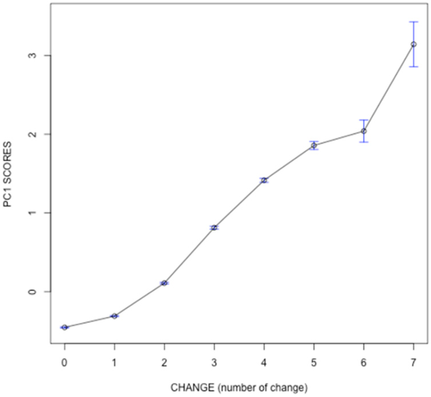
3.3. PC1 and Number of Changes in Biophysical Trends

The change information was utilized to interpret the first component by performing a univariate general linear model (LM1) between PC1 scores and the number of changes, as determined by the SDTC [5]. The change categories correspond to the number of changing STA Fourier parameters in a segment. Results illustrate that the average scores increase when the number of changing parameters increases (Figure 8) and that the LM1 correlation between the change variable and PC1 is high with a value of 0.553 (p < 0.001). Evidence is consistent with expectations: pixels with higher scores have many significant changing shape parameters, and the higher the PC1 score, the more the changes in STA found.
Figure 8. Average PC1 score for the CHANGE variable with 95% confidence intervals: this indicates that the mean scores for PC1 increase when the number of significant changes increases.
Remotesensing 06 12639 g008

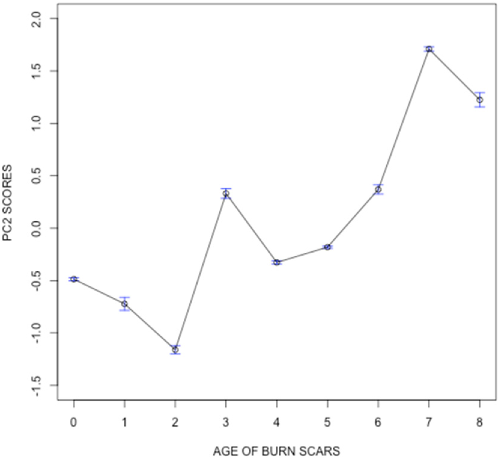
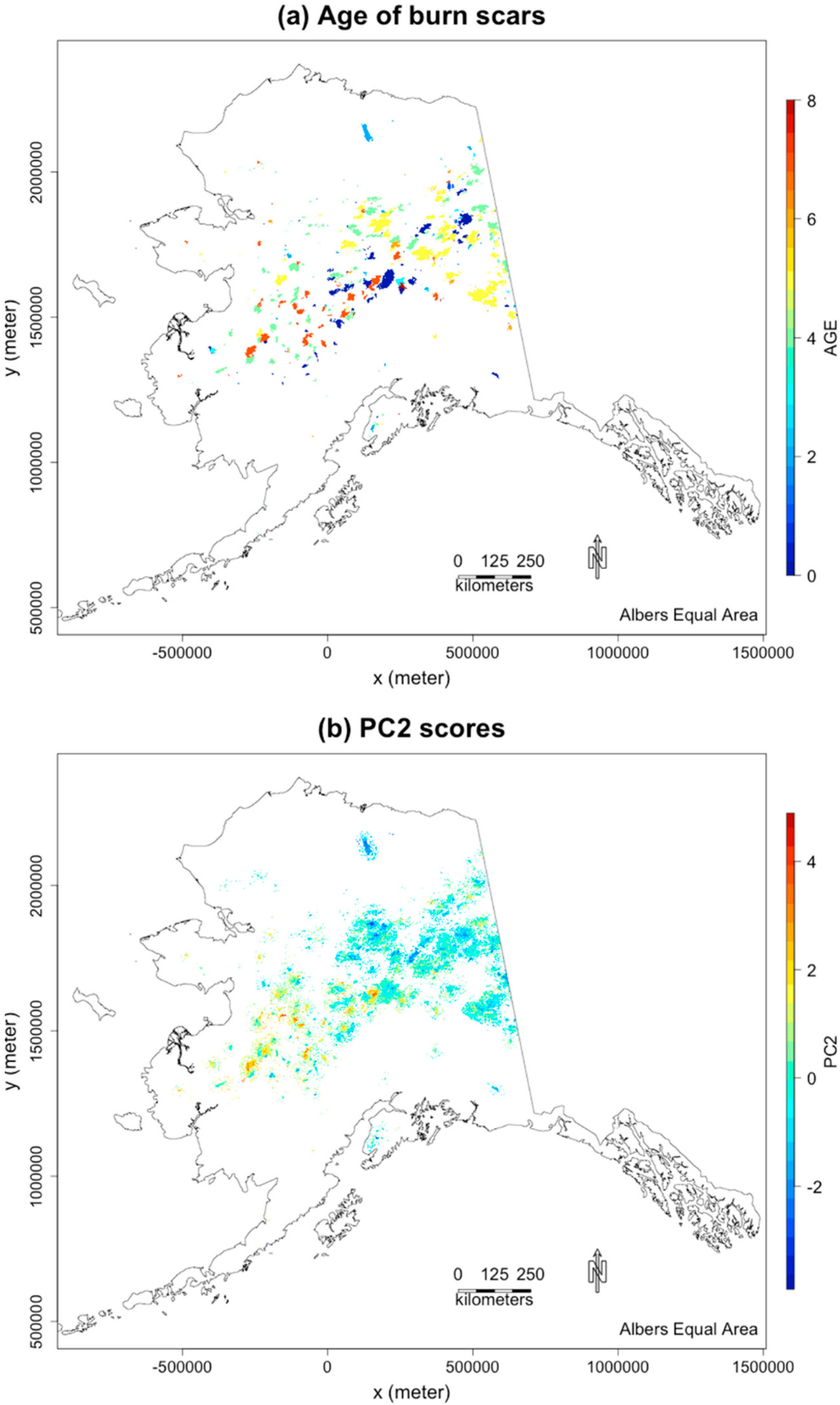
3.4. PC2 and Burn Scar Age

The second principal component (PC2) was interpreted using the “age” of burned areas created using the MTBS database. The LM1 correlation between the variables age and PC2 is 0.422 (p < 0.001) (on burned pixel areas only). The relationship is visualized by plotting the average scores for every age class in burned areas (Figure 9) and mapping both variables (Figure 10). Results indicate that PC2 scores are positive for old burned areas, i.e., burned areas occurring at the beginning of the time series, and negative for young burned areas (at the end of the time series). Taking into account loading patterns (Figure 3), PC2 can be interpreted in the following way: high positive score pixels show increases in NDVI_A1 with decreases in LST_A0, while low negative score pixels show the reverse trends. Thus, the results suggest that that old age burn scar shows an increase in annual NDVI seasonal variability (NDVI_A1) and a decrease in average land surface temperature (LST_A0), while recent burn scars display a decrease in NDVI_A1 and an increase in LST_A0.
Figure 9. Average PC2 scores with 95% confidence interval: the average PC2 score increases when the age of the burned areas increases.
Remotesensing 06 12639 g009
Figure 10. Map of age for burn scars (a) and PC2 scores (b).
Remotesensing 06 12639 g010

3.5. Discussions

Using validation/ancillary datasets, we found that STA with PCA can be used to extract meaningful temporal patterns related to land transitions caused by fire disturbance. More specifically, results indicate that the first principal component (PC1) relates to fire occurrence (Boolean “BURNED” variable), fire severity (dNBR) and the number of changing Fourier parameters, as well as a combination of four Fourier trends (ALB_A0, ALB_A1, LST_A1 and NDVI_A0). At this stage, it is important to highlight a few important points.
First, it is implicit in the analysis that space can be substituted for time. Indeed, PCA results display differences in trends between burned and unburned pixels. Thus, it is assumed that when a pixel transitions from an unburned to a burned state, changes in its temporal annual trajectory will be indicated by its Fourier trend parameters.
Second, PCA on the Fourier parameters tackles the first research question: What combination of trends in surface variables characterizes change areas that transitioned from the unburned to burned category? It is important to note that PCA is carried out using the correlation matrix to account for different variables scaling and to focus on the characteristic of change. Thus, the sign of the slopes must be considered with care whenever interpreting the results, because the reference is the average rather than the value zero for an uncentered analysis [83]. This means that pixels with high positive scores possess TS slopes higher than average for ALB_A0, ALB_A1 and LST_A1, but the values of the slopes may be positive for both the burned and unburned pixels in some cases. In fact, the analysis shows that only NDVI_A0 displays a change of sign (Figure 10). In order to further understand this interpretation, a LM1 analysis was carried out on the four individual Fourier variables that contribute the most to PC1 (NDVI_A0, ALB_A0, ALB_A1 and LST_A1). LM1 illustrates the changes in the TS slopes occurring when pixels transition from an unburned (value of zero) to burned state (value of one). The plots of average scores indicate that unburned pixels have low positive trends in ALB_A0 and ALB_A1 and that the TS slopes increase strongly when pixels transition to the burned category (Figure 11). This implies that pixels that transitioned display an increase in average albedo (ALB_A0), as well as an increase in the seasonal amplitude (ALB_A1).
Trend values for LST_A1 are somewhat peculiar, because the unburned pixels have high positive TS slopes. NDVI_A0 is the only parameter that displays a decrease in the TS slope when fire occurs (Figure 11a). The relative magnitude of transitions becomes clearer when the changes in TS slopes are reported in terms of percentages. Results indicate that there are large increases of nearly 500% for variables ALB_A0 and ALB_1, a large decrease of 800% for NDVI_A0 and a small increase of 38% for LST_A1.
Third, it was highlighted that burned pixels have a positive average score of 0.589 compared to −0.581 for unburned pixels. Higher average scores correspond to pixels with stronger biophysical changes that are better examples of fire transitions. In addition, within a burn scar, there exists a distribution of scores reflecting variation in burn severity.
The trends detected are in line with the expectation from the literature. We find that fire decreases the greenness/photosynthetic activity as measured by NDVI_A0. The increase in average albedo (ALB_A0) and albedo seasonality (ALB_A1) also match our expectation, since vegetation cover lowers albedo of surfaces by allowing the ground surfaces to have more patches of darker surfaces, particularly under snowy conditions [55]. We also find a general increase in temperature seasonality (LST_A1), which was also observed in Kaufman et al. [54]. The change in LST seasonality also makes sense since vegetation acts as a buffer for seasonal differences. Using ancillary data, we also find that when biophysical changes are stronger, they relate to higher fire severity, as measured by the dNBR index. PC1 could be used as an indicator describing the most important characteristic surfaces changes caused by fire disturbances in Alaska.
Figure 11. Patterns of change in STA trends with average and 95% confidence interval for all change (category 1) and no-change (category 0) areas (burned and unburned pixels) for the four variables that contribute the most to PC1. Note the transition is characterized by: (a) a decrease in NDVI_A0, (b) an increase in ALB_A0, (c) an increase in ALB1, (d) an increase in LST_A1.
Remotesensing 06 12639 g011

3.6. Uncertainties and Accuracy of the Analysis

While the results are solid in terms of the broad characterization of change, more work will be needed to evaluate the uncertainty of the method and its limitations. First, we used all of the change data (MTBS fire polygons), because the research focuses on the characterization of a priori known change areas and their contrast with control data in the direct vicinity. Results suggest that PC1 provides separability between burned and unburned pixels (Figure 3) and may be useful for prediction or classification. This possibility may be explored by separating the fire dataset into multiple training and testing datasets to validate the strength of the method in predicting and characterizing burned areas. Second, due to its focus on characterization, the STA-PCA method does not provide a statement about the significance of changes or its uncertainty, even though we found that the higher score implied a higher severity of change (in the context of fire). These two points can be ameliorated by using the SDTC method to detect areas that are changing without a priori information (i.e., burn information) and by using the number of changing parameters as a statement of uncertainty. Making a combined statement on the statistical significance of uncertainty is, however, complex, given the correlation among variables and the spatial autocorrelation between observations, and will require more methodological work in the future. An additional limitation of the method may come in dealing with the large variability in space and within areas of change. While using control data, we are able to show significant biophysical changes in p-value term between burned and unburned observations, we also find that the change class exhibits a large variance for some variables (in particular, ALB_A1 and LST_A1). This variance is most likely related to land cover, spatial heterogeneity or local differences in fire severity. We used ancillary information on land cover information to explore some of this variability. If PC1 is used a posteriori to extract clusters undergoing similar changes, this may become problematic in the context of prediction. This issue of variability and its effect on separability and characterization of change should be explored in future research.

4. Conclusions

Most studies have focused on the detection of land cover change rather than the characterization of biophysical changes in change areas. Tracking how surface attributes are altered by land cover change processes is important for environmental change studies, because surface changes can affect fluxes of energy, water and biogeochemical cycles and, in turn, impact directly or indirectly the local, as well as regional climate and environment. In this study, a procedure that combines STA and PCA is introduced to characterize land cover change associated with fire disturbances in Alaska using MODIS multivariate time series of three surface state variables, NDVI, albedo and LST, over the 2001–2009 time period. We use Alaska as a case study, as surface changes in the region have a large impact on the regional fluxes and the fire regime is expected to be affected by climate change. To characterize change, we use STA to model temporal patterns in short and noisy multivariate time series by extracting nine Fourier parameters related to the seasonality of biophysical attributes. As the number of variables increase, it becomes difficult to extract the most important patterns, because of the high number of variables and the potential complexity of the relationship. We therefore use PCA, with burned and unburned locations as the control, to synthetize and characterize biophysical changes over the state of Alaska.
The research is promising and highlights four main findings:
(1) The findings provide empirical evidence of multivariate biophysical changes associated with fire disturbances at the landscape level. The biophysical changes are consistent with the literature: there is an average 800% decrease in NDVI, an average 500% increase in albedo and its annual variability, as well as a concurrent average 38% increase in the annual variability of land surface temperature.
(2) The first principal component contains 35% of the variance and highlights biophysical trends in land change areas that can be related to the fire severity variable as measured by dNBR (Pearson correlation of 0.5). In addition, burned areas with a higher proportion of evergreen forest in 2001 are associated with higher PC1 scores, i.e., stronger biophysical changes.
(3) The first component also relates to change areas, as determined using the segment-based detection of trends and change (SDTC), with higher scores correlated to an increasing number of significant biophysical trends (a correlation of 0.55).
(4) The second component relates to the age of the burned areas and describes changes related to NDVI_A1, LST_A0. Recently, burned pixels were characterized by a strong decrease in the annual variability of NDVI and an increase in average temperature, while the reverse is true for older burned areas.
The interpretation of the results from the STA-PCA methods appears to be solid, with temporal patterns in agreement with the literature on fire disturbance. While we were able to extract meaningful patterns, a remaining challenge may be to evaluate the uncertainty of the results [16] and the significance of the trends. One way forward is to use the number of trends detected as changing from the SDTC method as further strong evidence of change and provide an estimate of uncertainty. These research avenues will be explored in future papers. Another limitation is that the method as currently presented requires a priori knowledge of change areas. If no change datasets are available, STA-PCA can be applied using change and no-change areas determined using the SDTC procedure (Parmentier and Eastman [5]). By combining STA-PCA with SDTC, it may be possible to provide an automatic detection of areas of change along with their temporal characterization. The study shows that collapsing information in change/no-change categorical variables hides much of the information contained in time series. Given the increasing availability of multiple times series for Earth monitoring, there is a need to improve methods to characterize surface changes to inform land change science. This research shows that there is a potential for researcher to provide both characterization and detection information to inform land change science.
Future plans include evaluating the procedure in other case study areas and with other types of land cover change. For instance, insect infestation and timber harvest may provide additional types of land cover changes to characterize in Alaska. The method is applicable more generally to other types of change, such as agricultural intensification, urbanization and deforestation in other geographical and climate areas. Beyond the extraction of patterns in and of itself, there is the potential for using the STA-PCA method to work from patterns to processes, by defining “signatures” of change from consistent and systematic combinations of seasonal trends related to specific land change processes. Thus, the results from this research provide systematic empirical evidence of surface changes associated with one type of change, fire disturbances, and suggest that STA with PCA may be used to characterize land cover change over a large landscape using temporal patterns from multivariate Earth observation time series.

Acknowledgments

I wish to thank Ronald Eastman for his input and feedback. Clark Labs provided the STA method and spatial analytical tools through the GIS software, Idrisi®. SPSS, R and Python were used for the statistical analyses and scripting.

Author Contributions

This research was conducted by Benoit Parmentier, including the design and conceptualization of the project, development of statistical methods, data processing algorithms and editing of the manuscript.

Conflicts of Interest

The author declares no conflict of interest.

References

  1. Franklin, S.E.; Wulder, M.A. Remote sensing methods in medium spatial resolution satellite data land cover classification of large areas. Prog. Phys. Geog. 2002, 26, 173–205. [Google Scholar] [CrossRef]
  2. Kulik, I.; Hornsby, K.S.; Bishop, I.D. Modeling geospatial trend changes in vegetation monitoring data. Comput. Environ. Urban Syst. 2011, 35, 45–56. [Google Scholar] [CrossRef]
  3. Wulder, M.A.; Franklin, S.E.; White, J.C. Sensitivity of hyperclustering and labelling land cover classes to landsat image acquisition date. Int. J. Remote Sens. 2004, 25, 5337–5344. [Google Scholar] [CrossRef]
  4. Coops, N.C.; Wulder, M.A.; White, J.C. 2 Identifying and describing forest disturbance and spatial pattern. In Understanding Forest Disturbance and Spatial Pattern; CRC Press: Boca Rocan, FL, USA, 2007; pp. 31–61. [Google Scholar]
  5. Parmentier, B.; Eastman, J.R. Land transitions from multivariate time series: Using seasonal trend analysis and segmentation to detect land-cover changes. Int. J. Remote Sens. 2014, 35, 671–692. [Google Scholar] [CrossRef]
  6. De Beurs, K.M.; Henebry, G.M. Land surface phenology and temperature variation in the international geosphere-biosphere program high-latitude transects. Glob. Change Biol. 2005, 11, 779–790. [Google Scholar] [CrossRef]
  7. Geng, L.; Ma, M.; Wang, X.; Yu, W.; Jia, S.; Wang, H. Comparison of eight techniques for reconstructing multi-satellite sensor time-series NDVI data sets in the heihe river basin, China. Remote Sens. 2014, 6, 2024–2049. [Google Scholar] [CrossRef]
  8. Hird, J.N.; McDermid, G.J. Noise reduction of NDVI time series: An empirical comparison of selected techniques. Remote Sens. Environ. 2009, 113, 248–258. [Google Scholar] [CrossRef]
  9. Kandasamy, S.; Baret, F.; Verger, A.; Neveux, P.; Weiss, M. A comparison of methods for smoothing and gap filling time series of remote sensing observations: Application to MODIS LAI products. Biogeosci. Discuss. 2012, 9, 17053–17097. [Google Scholar] [CrossRef]
  10. Musial, J.P.; Verstraete, M.M.; Gobron, N. Technical note: Comparing the effectiveness of recent algorithms to fill and smooth incomplete and noisy time series. Atmos. Chem. Phys. 2011, 11, 7905–7923. [Google Scholar] [CrossRef] [Green Version]
  11. Eastman, J.R.; Sangermano, F.; Ghimire, B.; Zhu, H.; Chen, H.; Neeti, N.; Cai, Y.; Machado, E.A.; Crema, S.C. Seasonal trend analysis of image time series. Int. J. Remote Sens. 2009, 30, 2721–2726. [Google Scholar] [CrossRef]
  12. Cihlar, J. Land cover mapping of large areas from satellites: Status and research priorities. Int. J. Remote Sens. 2000, 21, 1093–1114. [Google Scholar] [CrossRef]
  13. Mildrexler, D.J.; Zhao, M.; Heinsch, F.A.; Running, S.W. A new satellite-based methodology for continental-scale disturbance detection. Ecol. Appl. 2007, 17, 235–250. [Google Scholar] [CrossRef] [PubMed]
  14. Quaife, T.; Quegan, S.; Disney, M.; Lewis, P.; Lomas, M.; Woodward, F. Impact of land cover uncertainties on estimates of biospheric carbon fluxes. Glob. Biogeochem. Cy. 2008, 22. [Google Scholar] [CrossRef]
  15. Coops, N.C.; Wulder, M.A.; Iwanicka, D. Large area monitoring with a MODIS-based disturbance index (DI) sensitive to annual and seasonal variations. Remote Sens. Environ. 2009, 113, 1250–1261. [Google Scholar] [CrossRef]
  16. Forkel, M.; Carvalhais, N.; Verbesselt, J.; Mahecha, M.D.; Neigh, C.S.; Reichstein, M. Trend change detection in NDVI time series: Effects of inter-annual variability and methodology. Remote Sens. 2013, 5, 2113–2144. [Google Scholar] [CrossRef]
  17. Verbesselt, J.; Hyndman, R.; Zeileis, A.; Culvenor, D. Phenological change detection while accounting for abrupt and gradual trends in satellite image time series. Remote Sens. Environ. 2010, 114, 2970–2980. [Google Scholar] [CrossRef]
  18. Jacquin, A.; Sheeren, D.; Lacombe, J.-P. Vegetation cover degradation assessment in madagascar savanna based on trend analysis of MODIS NDVI time series. Int. J. Appl. Earth Obs. Geoinf. 2010, 12, S3–S10. [Google Scholar] [CrossRef]
  19. Lambin, E. Land-cover categories versus biophysical attributes to monitor land-cover change by remote sensing. In Observing Land from Space: Science, Customers and Technology; Springer Netherlands: Berlin, Germany, 2000; pp. 137–142. [Google Scholar]
  20. Kabat, P. Vegetation, Water, Humans and the Climate: A New Perspective on an Internactive System; Springer: New York, NY, USA, 2004. [Google Scholar]
  21. Lambin, E.F. Monitoring forest degradation in tropical regions by remote sensing: Some methodological issues. Globalecol. Biogeogr. 1999, 8, 191–198. [Google Scholar] [CrossRef]
  22. Monteith, J.; Unsworth, M. Principles of Environmental Physics: Plants, Animals, and the Atmosphere, 4th ed.; Academic Press: Salt Lake City, UT, USA, 2013. [Google Scholar]
  23. Swann, A.L.; Fung, I.Y.; Levis, S.; Bonan, G.B.; Doney, S.C. Changes in Arctic Vegetation Amplify High-Latitude Warming through the Greenhouse Effect. Available online: http://www.pnas.org/content/107/4/1295.full (accessed on 26 January 2010).
  24. Betts, R.A. Offset of the potential carbon sink from boreal forestation by decreases in surface albedo. Nature 2000, 408, 187–190. [Google Scholar] [CrossRef] [PubMed]
  25. Chapin, F.S., 3rd; Sturm, M.; Serreze, M.C.; McFadden, J.P.; Key, J.R.; Lloyd, A.H.; McGuire, A.D.; Rupp, T.S.; Lynch, A.H.; Schimel, J.P.; et al. Role of land-surface changes in arctic summer warming. Science 2005, 310, 657–660. [Google Scholar] [CrossRef] [PubMed]
  26. Lambin, E.F.; Geist, H.J. Land-Use and Land-Cover Change; Springer: New York, NY, USA, 2006. [Google Scholar]
  27. Bunn, A.G.; Goetz, S.J. Trends in satellite-observed circumpolar photosynthetic activity from 1982 to 2003: The influence of seasonality, cover type, and vegetation density. Earth Interact. 2006, 10, 1–19. [Google Scholar] [CrossRef]
  28. Hinzman, L.D.; Bettez, N.D.; Bolton, W.R.; Chapin, F.S.; Dyurgerov, M.B.; Fastie, C.L.; Griffith, B.; Hollister, R.D.; Hope, A.; Huntington, H.P. Evidence and implications of recent climate change in Northern Alaska and other arctic regions. Clim. Change 2005, 72, 251–298. [Google Scholar] [CrossRef]
  29. Myers-Smith, I.H.; Forbes, B.C.; Wilmking, M.; Hallinger, M.; Lantz, T.; Blok, D.; Tape, K.D.; Macias-Fauria, M.; Sass-Klaassen, U.; Lévesque, E. Shrub expansion in tundra ecosystems: Dynamics, impacts and research priorities. Environ. Res. Lett. 2011, 6. [Google Scholar] [CrossRef]
  30. Lupo, F.; Linderman, M.; Vanacker, V.; Bartholome, E.; Lambin, E. Categorization of land-cover change processes based on phenological indicators extracted from time series of vegetation index data. Int. J. Remote Sens. 2007, 28, 2469–2483. [Google Scholar] [CrossRef]
  31. Kennedy, R.E.; Cohen, W.B.; Schroeder, T.A. Trajectory-based change detection for automated characterization of forest disturbance dynamics. Remote Sens. Environ. 2007, 110, 370–386. [Google Scholar] [CrossRef]
  32. Sparks, T.H.; Menzel, A. Observed changes in seasons: An overview. Int. J. Climatol. 2002, 22, 1715–1725. [Google Scholar] [CrossRef]
  33. Torrence, C.; Compo, G.P. A practical guide to wavelet analysis. B. Am. Meteorol. Soc. 1998, 79, 61–78. [Google Scholar] [CrossRef]
  34. Jakubauskas, M.E.; Legates, D.R.; Kastens, J.H. Harmonic Analysis of Time-Series AVHRR NDVI Data. Available online: http://kbs.ku.edu/media/uploads/work/Jakubauskas_PERS2001_Harmonic_analysis_of_time-series_AVHRR_NDVI_data.pdf (accessed on 5 October 2014).
  35. Moody, A.; Johnson, D.M. Land-surface phenologies from AVHRR using the discrete fourier transform. Remote Sens. Environ. 2001, 75, 305–323. [Google Scholar] [CrossRef]
  36. Theil, H. A Rank-Invariant Method of Linear and Polynomial Regression Analysis; Springer Netherlands: Berlin, Germany, 1950. [Google Scholar]
  37. Sen, P.K. Estimates of the regression coefficient based on kendall’s tau. J. Am. Stat. Assoc. 1968, 63, 1379–1389. [Google Scholar] [CrossRef]
  38. Eastman, J.R. Idrisi Taiga Guide to GIS and Image Processing; Clark University: Worcester, MA, USA, 2009. [Google Scholar]
  39. Eastman, J.R.; Sangermano, F.; Machado, E.A.; Rogan, J.; Anyamba, A. Global trends in seasonality of Normalized Difference Vegetation Index (NDVI), 1982–2011. Remote Sens. 2013, 5, 4799–4818. [Google Scholar] [CrossRef]
  40. Liu, H.; Randerson, J.T.; Lindfors, J.; Chapin, F.S., III. Changes in the surface energy budget after fire in boreal ecosystems of interior Alaska: An annual perspective. J. Geophys. Res. 2005, 110. [Google Scholar] [CrossRef]
  41. Randerson, J.T.; Liu, H.; Flanner, M.G.; Chambers, S.D.; Jin, Y.; Hess, P.G.; Pfister, G.; Mack, M.C.; Treseder, K.K.; Welp, L.R.; et al. The impact of boreal forest fire on climate warming. Science 2006, 314, 1130–1132. [Google Scholar] [CrossRef] [PubMed]
  42. Johnstone, J.F.; Hollingsworth, T.N.; Chapin, F.S.; Mack, M.C. Changes in fire regime break the legacy lock on successional trajectories in Alaskan boreal forest. Glob. Change Biol. 2010, 16, 1281–1295. [Google Scholar] [CrossRef]
  43. Epting, J.; Verbyla, D. Landscape-level interactions of prefire vegetation, burn severity, and postfire vegetation over a 16-year period in interior Alaska. Can. J. Forest Res. 2005, 35, 1367–1377. [Google Scholar] [CrossRef]
  44. Chambers, S.; Chapin, F. Fire effects on surface-atmosphere energy exchange in Alaskan black spruce ecosystems: Implications for feedbacks to regional climate. J. Geophys. Res. 2003, 108. [Google Scholar] [CrossRef]
  45. Kasischke, E.; French, N. Constraints on using avhrr composite index imagery to study patterns of vegetation cover in boreal forests. Int. J Remote Sens. 1997, 18, 2403–2426. [Google Scholar] [CrossRef]
  46. Lyons, E.A.; Jin, Y.; Randerson, J.T. Changes in surface albedo after fire in boreal forest ecosystems of interior Alaska assessed using MODIS satellite observations. J. Geophys. Res. Biogeosci. 2008, 113. [Google Scholar] [CrossRef]
  47. Kasischke, E.S.; Bourgeau-Chavez, L.L.; Johnstone, J.F. Assessing spatial and temporal variations in surface soil moisture in fire-disturbed black spruce forests in interior Alaska using spaceborne synthetic aperture radar imagery—Implications for post-fire tree recruitment. Remote Sens. Environ. 2007, 108, 42–58. [Google Scholar] [CrossRef]
  48. Bourgeau-Chavez, L.; Kasischke, E.; Riordan, K.; Brunzell, S.; Nolan, M.; Hyer, E.; Slawski, J.; Medvecz, M.; Walters, T.; Ames, S. Remote monitoring of spatial and temporal surface soil moisture in fire disturbed boreal forest ecosystems with ERS SAR imagery. Int. J. Remote Sens. 2007, 28, 2133–2162. [Google Scholar] [CrossRef]
  49. Balshi, M.S.; McGuire, A.D.; Zhuang, Q.; Melillo, J.; Kicklighter, D.W.; Kasischke, E.; Wirth, C.; Flannigan, M.; Harden, J.; Clein, J.S.; et al. The role of historical fire disturbance in the carbon dynamics of the pan-boreal region: A process-based analysis. J. Geophys. Res. 2007, 112. [Google Scholar] [CrossRef]
  50. Foley, J.A. Tipping points in the tundra. Science 2005, 310, 627–628. [Google Scholar] [CrossRef] [PubMed]
  51. Lambin, E.F.; Ehrlich, D. Land-cover changes in sub-Saharan Africa (1982–1991): Application of a change index based on remotely sensed surface temperature and vegetation indices at a continental scale. Remote Sens. Environ. 1997, 61, 181–200. [Google Scholar] [CrossRef]
  52. Nemani, R.; Running, S. Land cover characterization using multitemporal red, near-IR, and thermal-IR data from NOAA/AVHRR. Ecol. Appl. 1997, 7, 79–90. [Google Scholar] [CrossRef]
  53. Julien, Y.; Sobrino, J.A. The yearly land cover dynamics (YLCD) method: An analysis of global vegetation from NDVI and LST parameters. Remote Sens. Environ. 2009, 113, 329–334. [Google Scholar] [CrossRef]
  54. Kaufmann, R.; Zhou, L.; Myneni, R.; Tucker, C.; Slayback, D.; Shabanov, N.; Pinzon, J. The effect of vegetation on surface temperature: A statistical analysis of ndvi and climate data. Geophys. Res. Lett. 2003, 30. [Google Scholar] [CrossRef]
  55. Betts, A.K.; Ball, J.H. Albedo over the boreal forest. J. Geophys. Res. Atmos. 1997, 102, 28901–28909. [Google Scholar] [CrossRef]
  56. Beck, P.S.A.; Goetz, S.J.; Mack, M.C.; Alexander, H.D.; Jin, Y.; Randerson, J.T.; Loranty, M.M. The impacts and implications of an intensifying fire regime on Alaskan boreal forest composition and albedo. Glob. Change Biol. 2011, 17, 2853–2866. [Google Scholar] [CrossRef]
  57. Susan, S. Climate Change 2007—The Physical Science Basis: Working Group I Contribution to the Fourth Assessment Report of the IPCC; Cambridge University Press: Cambridge, UK, 2007. [Google Scholar]
  58. Serreze, M.; Walsh, J.; Chapin, F.S.; Osterkamp, T.; Dyurgerov, M.; Romanovsky, V.; Oechel, W.; Morison, J.; Zhang, T.; Barry, R. Observational evidence of recent change in the northern high-latitude environment. Clim. Change 2000, 46, 159–207. [Google Scholar] [CrossRef]
  59. Angert, A.; Biraud, S.; Bonfils, C.; Henning, C.; Buermann, W.; Pinzon, J.; Tucker, C.; Fung, I. Drier Summers Cancel out the CO2 Uptake Enhancement induced by Warmer Springs. Available online: http://www.pnas.org/content/102/31/10823.full (accessed on 2 August 2005).
  60. Osterkamp, T.; Romanovsky, V. Evidence for warming and thawing of discontinuous permafrost in Alaska. Permafrost Periglac. 1999, 10, 17–37. [Google Scholar] [CrossRef]
  61. Jorgenson, M.T.; Racine, C.H.; Walters, J.C.; Osterkamp, T.E. Permafrost degradation and ecological changes associated with a warming climate in Central Alaska. Clim. Change 2001, 48, 551–579. [Google Scholar] [CrossRef]
  62. Yoshikawa, K.; Hinzman, L.D. Shrinking thermokarst ponds and groundwater dynamics in discontinuous permafrost near council, Alaska. Permafrost Periglac. 2003, 14, 151–160. [Google Scholar] [CrossRef]
  63. Malmström, C.M.; Raffa, K.F. Biotic disturbance agents in the boreal forest: Considerations for vegetation change models. Glob. Change Biol. 2002, 6, 35–48. [Google Scholar] [CrossRef]
  64. Dale, V.H.; Joyce, L.A.; McNulty, S.; Neilson, R.P.; Ayres, M.P.; Flannigan, M.D.; Hanson, P.J.; Irland, L.C.; Lugo, A.E.; Peterson, C.J.; et al. Climate change and forest disturbances. BioScience 2001, 51, 723–734. [Google Scholar] [CrossRef]
  65. Kasischke, E.S.; Verbyla, D.L.; Rupp, T.S.; McGuire, A.D.; Murphy, K.A.; Jandt, R.; Barnes, J.L.; Hoy, E.E.; Duffy, P.A.; Calef, M.; et al. Alaska’s changing fire regime—Implications for the vulnerability of its boreal forests. Can. J. Forest Res. 2010, 40, 1313–1324. [Google Scholar] [CrossRef]
  66. Turetsky, M.R.; Kane, E.S.; Harden, J.W.; Ottmar, R.D.; Manies, K.L.; Hoy, E.; Kasischke, E.S. Recent acceleration of biomass burning and carbon losses in Alaskan forests and peatlands. Nat. Geosci. 2010, 4, 27–31. [Google Scholar] [CrossRef]
  67. Tape, K.E.N.; Sturm, M.; Racine, C. The evidence for shrub expansion in Northern Alaska and the pan-arctic. Glob. Change Biol. 2006, 12, 686–702. [Google Scholar] [CrossRef]
  68. Chapin, F.S., III; Oswood, M.W.; Van Cleve, K.; Verbyla, D. Alaska Changing Boreal Forest; Oxford University Press: New York, NY, USA, 2006. [Google Scholar]
  69. Harden, J.; Trumbore, S.; Stocks, B.; Hirsch, A.; Gower, S.; O’neill, K.; Kasischke, E. The role of fire in the boreal carbon budget. Glob. Change Biol. 2002, 6, 174–184. [Google Scholar] [CrossRef]
  70. Shenoy, A.; Johnstone, J.F.; Kasischke, E.S.; Kielland, K. Persistent effects of fire severity on early successional forests in interior Alaska. Forest Ecol. Manag. 2011, 261, 381–390. [Google Scholar] [CrossRef]
  71. Bachelet, D.; Lenihan, J.; Neilson, R.; Drapek, R.; Kittel, T. Simulating the response of natural ecosystems and their fire regimes to climatic variability in Alaska. Can. J. Forest Res. 2005, 35, 2244–2257. [Google Scholar] [CrossRef]
  72. Olson, D.M.; Dinerstein, E.; Wikramanayake, E.D.; Burgess, N.D.; Powell, G.V.; Underwood, E.C.; D'amico, J.A.; Itoua, I.; Strand, H.E.; Morrison, J.C. Terrestrial ecoregions of the world: A new map of life on earth a new global map of terrestrial ecoregions provides an innovative tool for conserving biodiversity. BioScience 2001, 51, 933–938. [Google Scholar] [CrossRef]
  73. Huete, A.; Didan, K.; Miura, T.; Rodriguez, E.P.; Gao, X.; Ferreira, L.G. Overview of the radiometric and biophysical performance of the MODIS vegetation indices. Remote Sens. Environ. 2002, 83, 195–213. [Google Scholar] [CrossRef]
  74. Wan, Z. MODIS Land-Surface Temperature Algorithm Theoretical Basis Document (LST ATBD). Available online: http://modis.gsfc.nasa.gov/data/atbd/atbd_mod11.pdf (accessed on 5 October 2014).
  75. Schaaf, C.B.; Gao, F.; Strahler, A.H.; Lucht, W.; Li, X.; Tsang, T.; Strugnell, N.C.; Zhang, X.; Jin, Y.; Muller, J.-P. First operational BRDF, albedo nadir reflectance products from MODIS. Remote Sens. Environ. 2002, 83, 135–148. [Google Scholar] [CrossRef]
  76. Land Processes Distributed Active Archive Center (LP DAAC). MODIS Data Products Table. Available online: https://lpdaac.usgs.gov/products/modis_products_table (accessed on 5 October 2014).
  77. MTBS. Monitoring Trends in Burn Severity. Available online: http://www.mtbs.gov/ (accessed on 10 December 2010).
  78. French, N.H.; Kasischke, E.S.; Hall, R.J.; Murphy, K.A.; Verbyla, D.L.; Hoy, E.E.; Allen, J.L. Using Landsat data to assess fire and burn severity in the North American boreal forest region: An overview and summary of results. Int. J. Wildland Fire 2008, 17, 443–462. [Google Scholar] [CrossRef]
  79. Homer, C.; Huang, C.; Yang, L.; Wylie, B.K.; Coan, M. Development of a 2001 national land-cover database for the United States. Photogramm. Eng. Remote Sens. 2004, 70. [Google Scholar] [CrossRef]
  80. Kasischke, E.S.; Hoy, E.E. Controls on carbon consumption during Alaskan wildland fires. Glob. Change Biol. 2012, 18, 685–699. [Google Scholar] [CrossRef]
  81. Neeti, N.; Eastman, J.R. A contextual mann-kendall approach for the assessment of trend significance in image time series. Trans. GIS 2011, 15, 599–611. [Google Scholar] [CrossRef]
  82. Hoaglin, D.C.M.; John, W. Understanding Robust and Exploratory Data Analysis; Wiley: New York, NY, USA, 2000. [Google Scholar]
  83. Jolliffe, I. Principal Component Analysis; Wiley Online Library: New York, NY, USA, 2005. [Google Scholar]
  84. Jaccard, J.; Turrisi, R. Interaction Effects in Multiple Regression; Sage Publications: Thousands Oaks, CA, USA, 2003. [Google Scholar]
  85. Eidenshink, J.; Schwind, B.; Brewer, K.; Zhu, Z.-L.; Quayle, B.; Howard, S. A Project for Monitoring Trends in Burn Severity. Available online: http://naldc.nal.usda.gov/naldc/download.xhtml?id=16261&content=PDF (accessed on 5 October 2014).
  86. Allen, J.L.; Sorbel, B. Assessing the differenced normalized burn ratio’s ability to map burn severity in the boreal forest and tundra ecosystems of Alaska’s national parks. Int. J. Wildland Fire 2008, 17, 463–475. [Google Scholar] [CrossRef]
  87. Hoy, E.E.; French, N.H.; Turetsky, M.R.; Trigg, S.N.; Kasischke, E.S. Evaluating the potential of Landsat TM/ETM+ imagery for assessing fire severity in Alaskan black spruce forests. Int. J. Wildland Fire 2008, 17, 500–514. [Google Scholar] [CrossRef]
  88. Murphy, K.A.; Reynolds, J.H.; Koltun, J.M. Evaluating the ability of the delta normalized burn ratio (DNBR) to predict ecologically significant burn severity in Alaskan boreal forests. Int. J. Wildland Fire 2008, 17, 490–499. [Google Scholar] [CrossRef]
  89. Kasischke, E.S.; Hyer, E.J.; Novelli, P.C.; Bruhwiler, L.P.; French, N.H.F.; Sukhinin, A.I.; Hewson, J.H.; Stocks, B.J. Influences of boreal fire emissions on northern hemisphere atmospheric carbon and carbon monoxide. Glob. Biogeochem. Cy. 2005, 19. [Google Scholar] [CrossRef]
  90. Duffy, P.A.; Epting, J.; Graham, J.M.; Rupp, T.S.; McGuire, A.D. Analysis of Alaskan burn severity patterns using remotely sensed data. Int. J. Wildland Fire 2007, 16, 277–284. [Google Scholar] [CrossRef]
  91. Kasischke, E.S.; Turetsky, M.R.; Ottmar, R.D.; French, N.H.; Hoy, E.E.; Kane, E.S. Evaluation of the composite burn index for assessing fire severity in Alaskan black spruce forests. Int. J. Wildland Fire 2008, 17, 515–526. [Google Scholar] [CrossRef]

