Downscaling Pesticide Use Data to the Crop Field Level in California Using Landsat Satellite Imagery: Paraquat Case Study

Abstract
:1. Introduction
2. Case Study: Paraquat
Overview


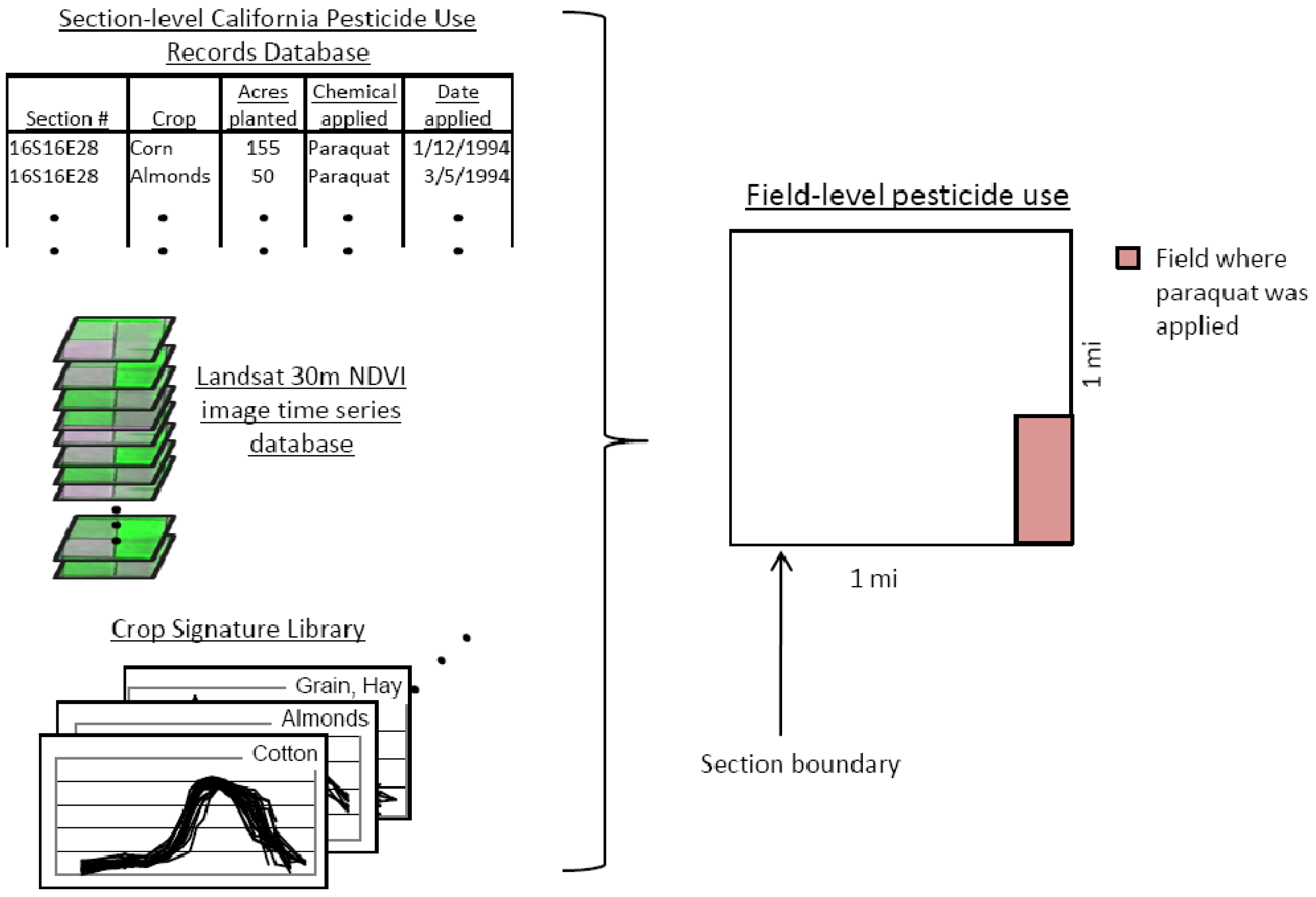
| Section # | Crop | Hectares Treated | Hectares Planted | Pounds Applied | Pounds/Hectare Applied | Date Applied |
|---|---|---|---|---|---|---|
| 14S17E01 | Vineyard | 8.1 | 8.1 | 17.3 | 2.14 | 20 February |
| 14S17E01 | Vineyard | 16.2 | 16.2 | 34.6 | 2.14 | 20 February |
| 16S17E01 | Cotton | 5.3 | 5.3 | 4.6 | 0.87 | 2 October |
| 17S17E01 | Cotton | 40.5 | 40.5 | 18.8 | 0.46 | 8 October |
| 18S17E01 | Cotton | 12.1 | 59.5 | 10.7 | 0.88 | 7 October |
| 18S17E01 | Cotton | 47.3 | 59.5 | 41.8 | 0.88 | 9 October |
| 18S17E01 | Cotton | 61.9 | 61.9 | 54.7 | 0.88 | 9 October |
| 18S17E01 | Cotton | 62.7 | 62.7 | 53.7 | 0.86 | 16 October |

3. Results and Discussion
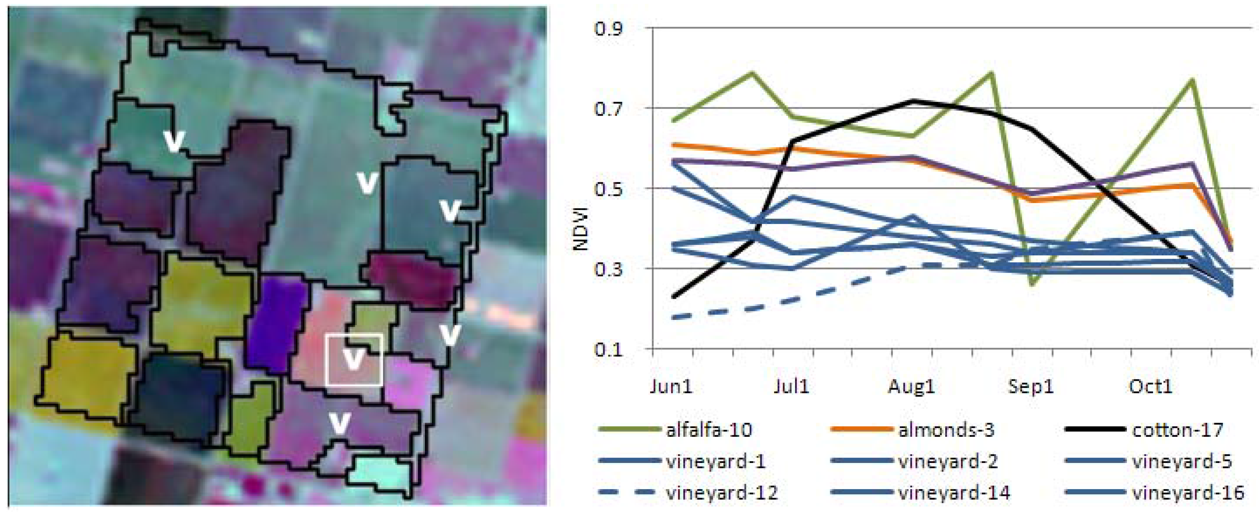
3.1. Section 14S17E01

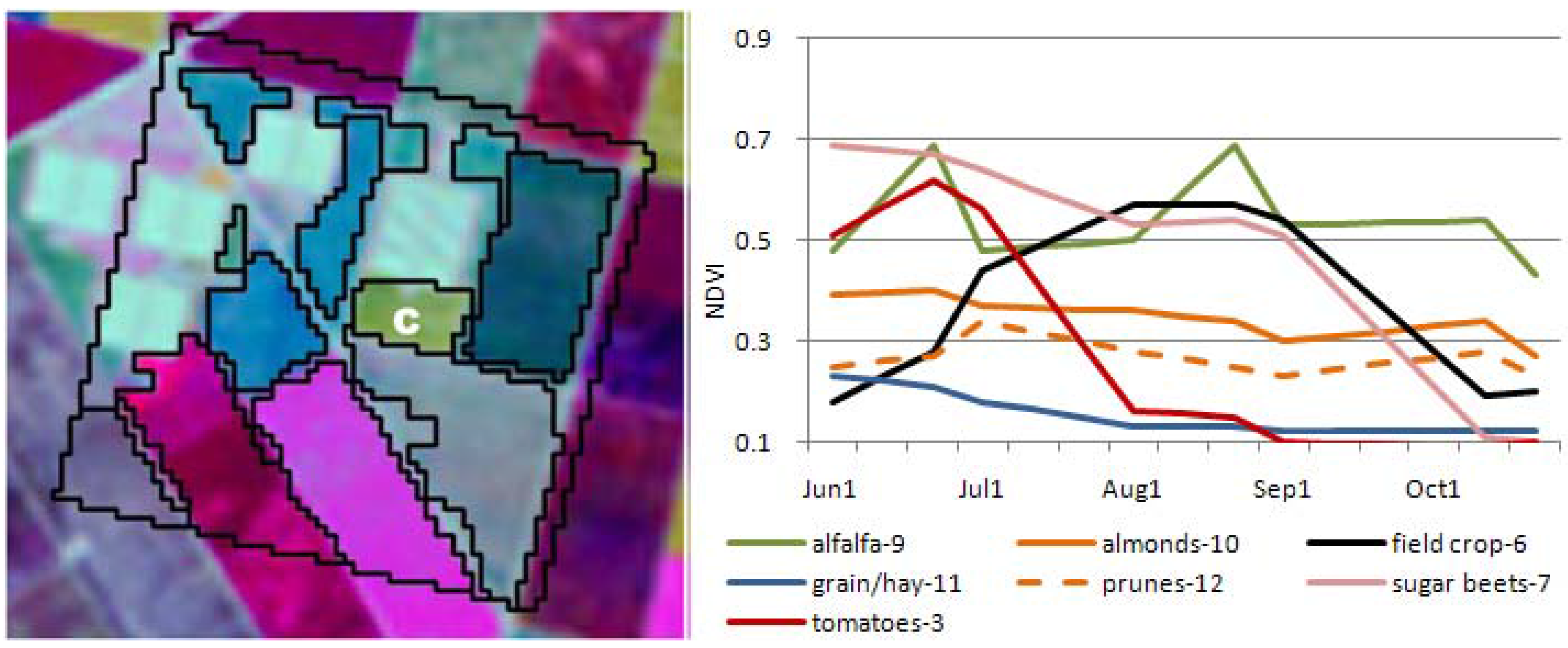
| Section #: 14S17E01 | Section #: 16S17E01 | |||||
|---|---|---|---|---|---|---|
| Field Unit | Median Difference | CDWR Class | Field Unit | Median Difference | CDWR Class | |
| FU16 | 0.03 | vineyard | FU6 | 0.34 | field crop | |
| FU1 | 0.04 | vineyard | FU9 | 0.41 | alfalfa | |
| FU14 | 0.05 | vineyard | FU10 | 0.81 | almonds | |
| FU2 | 0.06 | vineyard | FU7 | 0.87 | sugar beets | |
| FU5 | 0.09 | vineyard | FU12 | 1.07 | prunes | |
| FU13 | 0.14 | cotton | FU2 | 1.16 | other ag | |
| FU12 | 0.17 | vineyard | FU5 | 1.32 | tomatoes | |
| FU6 | 0.31 | walnuts | FU4 | 1.61 | tomatoes | |
| FU15 | 0.32 | field crop | FU1 | 1.71 | tomatoes | |
| FU3 | 0.34 | almonds | FU3 | 1.88 | tomatoes | |
| FU8 | 0.39 | cotton | FU8 | 1.92 | tomatoes | |
| FU7 | 0.39 | almonds | FU11 | 1.96 | grain/hay | |
| FU4 | 0.40 | almonds | ||||
| FU11 | 0.40 | alfalfa | ||||
| FU17 | 0.44 | cotton | ||||
| FU9 | 0.71 | cotton | ||||
| FU10 | 0.94 | alfalfa | ||||
| Section #: 17S17E01 | Section #: 18S17E01 | |||||
| Field Unit | Median Difference | CDWR Class | Field Unit | Median Difference | CDWR Class | |
| FU3 | 0.10 | cotton | FU2 | 0.08 | Cotton | |
| FU1 | 1.30 | grain/hay | FU1 | 0.09 | Cotton | |
| FU2 | 2.84 | grain/hay | FU4 | 1.52 | Safflower | |
| FU3 | 2.12 | Tomatoes | ||||
3.2. Section 16S17E01

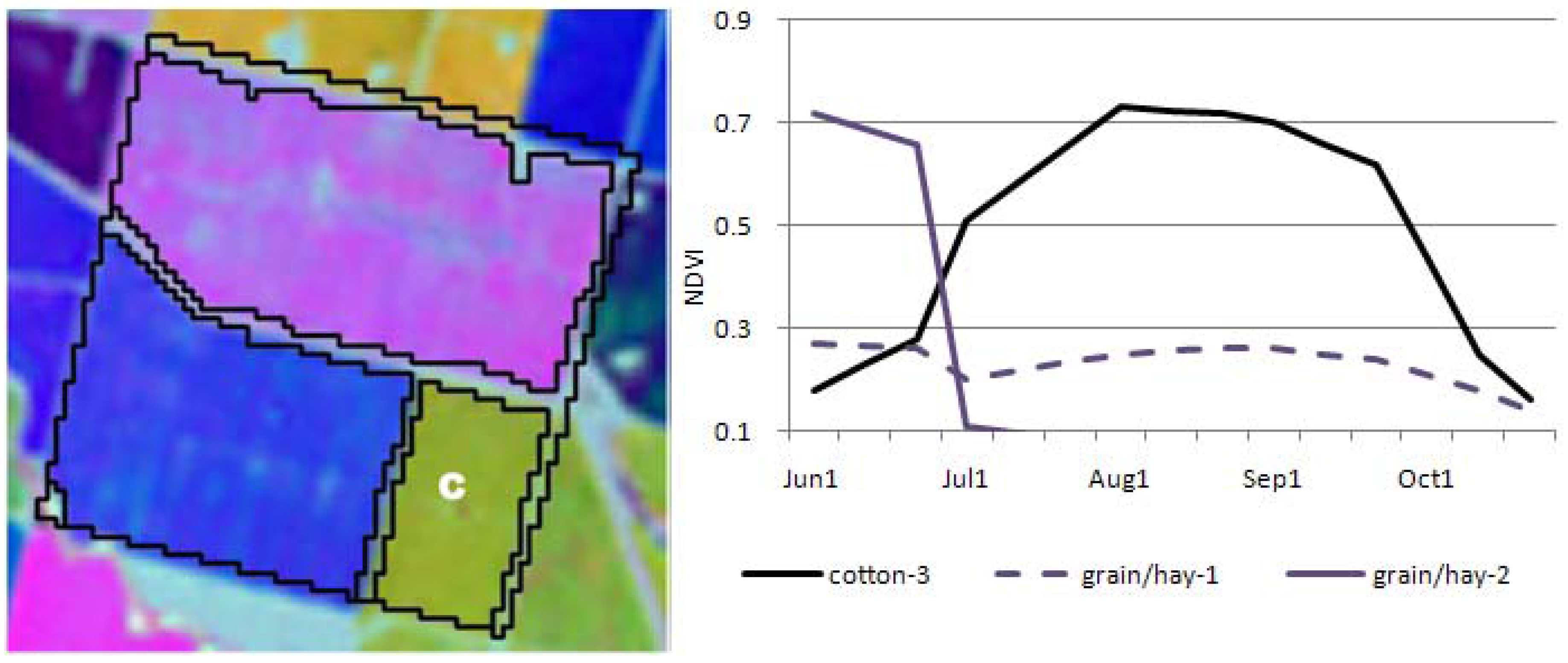
3.3. Section 17S17E01
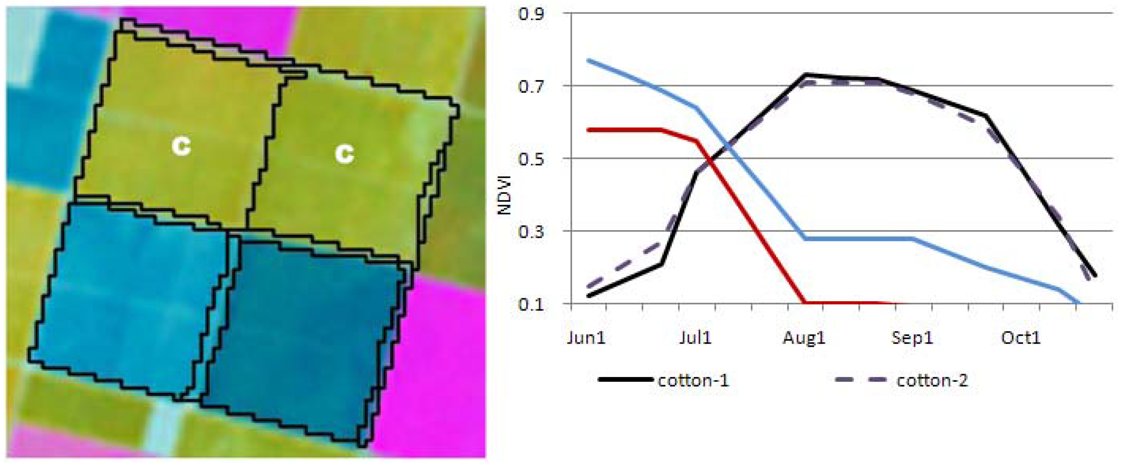
3.4. Section 18S17E01


3.5. Summary
4. Conclusions
Acknowledgments
References
- Daniels, J.L.; Olshan, A.F.; Savitz, D.A. Pesticides and childhood cancers. Environ. Health Perspect. 1997, 105, 1068–1077. [Google Scholar] [CrossRef] [PubMed]
- Infante-Rivard, C.; Weichenthal, S. Pesticides and childhood cancer: an update of Zahm and Ward’s 1998 review. J. Toxicol. Environ. Health B 2007, 10, 81–99. [Google Scholar] [CrossRef] [PubMed]
- Carozza, S.E.; Li, B.; Wang, Q.; Horel, S.; Cooper, S. Agricultural pesticides and risk of childhood cancers. Int. J. Hyg. Environ. Health 2009, 212, 186–195. [Google Scholar] [CrossRef] [PubMed]
- Turner, M.C.; Wigle, D.T.; Krewski, D. Residential pesticides and childhood leukemia: A systematic review and meta-analysis. Environ. Health Perspect. 2010, 118, 33–41. [Google Scholar] [PubMed]
- Weichenthal, S.; Moase, C.; Chan, P. A review of pesticide exposure and cancer incidence in the Agricultural Health Study cohort. Environ. Health Perspect. 2010, 118, 1117–1125. [Google Scholar] [CrossRef] [PubMed]
- Rull, R.P.; Ritz, B.; Shaw, G.M. Validation of self-reported proximity to agricultural crops in a case-control study of neural tube defects. J. Expo. Sci. Environ. Epidemiol. 2006, 16, 147–155. [Google Scholar] [CrossRef] [PubMed]
- Ritz, B.R.; Manthripragada, A.D.; Costello, S.; Lincoln, S.J.; Farrer, M.J.; Cockburn, M.; Bronstein, J. Dopamine transporter genetic variants and pesticides in Parkinson’s disease. Environ. Health Perspect. 2009, 117, 964–969. [Google Scholar] [CrossRef] [PubMed]
- Tanner, C.M.; Kamel, F.; Ross, G.W.; Hoppin, J.A.; Goldman, S.M.; Korell, M.; Marras, C.; Bhudhikanok, G.S.; Kasten, M.; Chade, A.R.; et al. Rotenone, Paraquat and Parkinson’s disease. Environ. Health Perspect. 2011, 119, 866–872. [Google Scholar] [CrossRef] [PubMed]
- Ward, M.H.; Lubin, J.; Giglierano, J.; Colt, J.S.; Wolter, C.; Bekiroglu, N.; Camann, D.; Hartge, P.; Nuckols, J.R. Proximity to crops and residential exposure to agricultural herbicides in Iowa. Environ. Health Perspect. 2006, 114, 893–897. [Google Scholar] [CrossRef] [PubMed]
- Nuckols, J.R.; Gunier, R.B.; Riggs, P.; Miller, R.; Reynolds, P.; Ward, M.H. Linkage of the California pesticide use reporting database with spatial land use data for exposure assessment. Environ. Health Perspect. 2007, 115, 684–689. [Google Scholar] [CrossRef] [PubMed]
- Gunier, R.B.; Ward, M.H.; Airola, M.; Bell, E.M.; Colt, J.; Nishioka, M.; Buffler, P.A.; Reynolds, P.; Rull, R.; Hertz, A.; et al. Determinants of agricultural pesticide concentrations in carpet dust. Environ Health Perspect. 2011, 119, 970–976. [Google Scholar] [CrossRef] [PubMed]
- California Department of Pesticide Reporting (CDPR). Pesticide Use Reporting: An overview of California’s Unique Full Reporting System; CDPR: Sacramento, CA, USA, 2000; p. 27. [Google Scholar]
- Rull, R.; Ritz, B. Historical pesticide exposure in California using pesticide use reports and land-use surveys: An assessment of misclassification error and bias. Environ. Health Perspect. 2003, 111, 1582–1589. [Google Scholar] [CrossRef] [PubMed]
- Riggs, P.D. Assessing Multiple Geospatial Modeling Techniques of Assigning Pesticide Exposure in the California Central Valley. Ph.D. Thesis, Colorado State University, Fort Collins, CO, USA, 2007. [Google Scholar]
- Costello, S.; Cockburn, M.G.; Bronstein, J.; Zhang, X.; Ritz, B. Parkinson disease and residential exposure to maneb and paraquat from agricultural applications in the Central Valley of California. Am. J. Epidemiol. 2009, 169, 919–926. [Google Scholar] [CrossRef] [PubMed]
- California Department of Water Resources (CDWR). California Land and Water Use; CDWR: Sacramento, CA, USA, 2009. Available online: http://www.water.ca.gov/landwateruse/lusrvymain.cfm (accessed on -15 June 2011).
- US Department of Agriculture (USDA). Weekly Weather and Crop Bulletin; Volume 87, No’s 1-52; National Agricultural Statistics Service, Agricultural Statistics Board, USDA: Washington, DC, USA, 2000. Available online: http://www.usda.gov/oce/weather/pubs/Weekly/Wwcb/index.htm (accessed on 15 June 2011).
- California Department of Water Resources (CDWR). California Water Plan Update; CDWR: Sacramento, CA, USA, 2009; pp. 160–209. [Google Scholar]
- Maxwell, S.K.; Airola, M.; Nuckols, J.R. Using Landsat satellite data to support pesticide exposure assessment in California. Int. J. Health Geogr. 2010, 9, 46. [Google Scholar] [CrossRef] [PubMed]
- Brody, J.G.; Vorhees, D.F.; Melly, S.J.; Swedis, S.R.; Drivas, P.J.; Rudel, R.A. Using GIS and historical records to reconstruct residential exposure to large-scale pesticide application. J. Expo. Anal. Environ. Epidemiol. 2002, 12, 64–80. [Google Scholar] [CrossRef] [PubMed]
- O’Leary, E.S.; Vena, J.E.; Freudenheim, J.L.; Brasure, J. Pesticide exposure and risk of breast cancer: A nested case-control study of residentially stable women living on Long Island. Environ. Res. 2004, 94, 134–144. [Google Scholar] [CrossRef] [PubMed]
- Ward, M.H.; Nuckols, J.R.; Weigel, S.J.; Maxwell, S.K.; Cantor, K.P.; Miller, R.S. Identifying populations potentially exposed to agricultural pesticides using remote sensing and a geographic information system. Environ Health Perspect. 2000, 108, 5–12. [Google Scholar] [CrossRef] [PubMed]
- US Geological Survey (USGS). Opening the Landsat Archive: US Geological Survey Fact Sheet 2008–3091; USGS: Reston, VA, USA, 2008; p. 1. [Google Scholar]
- Neumeister, L.; Isenring, R. Paraquat. Unacceptable Health Risks for Users, 3rd ed.; Berne Declaration, Pesticide Action Network UK, PAN Asia and the Pacific; 2011. [Google Scholar]
- California Department of Pesticide Regulation, California Pesticide Information Portal. Available online: http://calpip.cdpr.ca.gov/main.cfm (accessed on 15 June 2011).
- US Geological Survey (USGS). In Global Visualization Viewer (GloVis) website. Available online: http://glovis.usgs.gov/ (accessed on 15 June 2011).
- Gamon, J.A.; Field, C.B.; Goulden, M.L.; Griffin, K.L.; Hartley, A.E.; Joel, G.; Penuelas, J.; Valentini, R. Relationships between NDVI, canopy structure, and photosynthesis in three Californian vegetation types. Ecol. Appl. 1995, 5, 28–41. [Google Scholar] [CrossRef]
- Wang, J.; Rich, P.M.; Price, K.P.; Kettle, W.D. Relations between NDVI, grassland production, and crop yield in the Central Great Plains. Geocarto Int. 2005, 20, 5–11. [Google Scholar] [CrossRef]
- Dobrowski, S.Z.; Safford, H.D.; Cheng, Y.B.; Ustin, S.L. Mapping mountain vegetation using species distribution modeling, image-based texture analysis, and object-based classification. Appl. Veg. Sci. 2008, 11, 499–508. [Google Scholar] [CrossRef]
- Maxwell, S.K. Generating land cover boundaries from remotely sensed data using object-based image analysis: Overview and epidemiological application. Spat. Spatio-Temporal Epidemiol. 2010, 1, 231–237. [Google Scholar] [CrossRef] [PubMed]
© 2011 by the authors; licensee MDPI, Basel, Switzerland. This article is an open access article distributed under the terms and conditions of the Creative Commons Attribution license (http://creativecommons.org/licenses/by/3.0/).
Share and Cite
Maxwell, S.K. Downscaling Pesticide Use Data to the Crop Field Level in California Using Landsat Satellite Imagery: Paraquat Case Study. Remote Sens. 2011, 3, 1805-1816. https://doi.org/10.3390/rs3091805
Maxwell SK. Downscaling Pesticide Use Data to the Crop Field Level in California Using Landsat Satellite Imagery: Paraquat Case Study. Remote Sensing. 2011; 3(9):1805-1816. https://doi.org/10.3390/rs3091805
Chicago/Turabian StyleMaxwell, Susan K. 2011. "Downscaling Pesticide Use Data to the Crop Field Level in California Using Landsat Satellite Imagery: Paraquat Case Study" Remote Sensing 3, no. 9: 1805-1816. https://doi.org/10.3390/rs3091805