
Evaluation of Blended Wind Products and Their Implications for Offshore Wind Power Estimation


1
Joint Institute for Regional Earth System Science and Engineering, University of California at Los Angeles, Los Angeles, CA 90095, USA
2
Jet Propulsion Laboratory, California Institute of Technology, Pasadena, CA 91109, USA
3
Remote Sensing Systems, Santa Rosa, CA 95401, USA
*
Author to whom correspondence should be addressed.
Remote Sens. 2023, 15(10), 2620; https://doi.org/10.3390/rs15102620
Submission received: 8 February 2023
/
Revised: 24 April 2023
/
Accepted: 14 May 2023
/
Published: 18 May 2023
Abstract
:The Cross-Calibrated Multi-Platform (CCMP) wind analysis is a satellite-based blended wind product produced using a two-dimensional variational method. The current version available publicly is Version 2 (CCMP2.0), which includes buoy winds in addition to satellite winds. Version 3 of the product (CCMP3.0) is being produced with several improvements in analysis algorithms, without including buoy winds. Here, we compare CCMP3.0 with a special version of CCMP2.0 that did not include buoy winds, so both versions are independent of buoy measurements. We evaluate them using wind data from buoys around the coasts of the United States and discuss the implications for the wind power industry and offshore wind farms. CCMP2.0 uses ERA-Interim 10 m winds as the background to fill observational gaps. CCMP3.0 uses ERA5 10 m neutral winds as the background. Because ERA5 winds are biased towards lower values at higher wind conditions, CCMP3.0 corrected this bias by matching ERA5 wind speeds with satellite scatterometer wind speeds using a histogram matching method. Our evaluation indicates that CCMP3.0 has better agreement with the independent buoy winds, primarily for higher winds (>10 m/s). This is reflected by the higher correlation and lower root-mean-squared differences of CCMP3.0 versus buoy winds, especially for higher wind conditions. For the U.S. coastal region (within 200 km), the mean wind speed of CCMP3.0 is enhanced by 1–2%, and the wind speed standard deviation is enhanced by around 3–5%. These changes in wind speed and its standard deviation from CCMP2.0 to CCMP3.0 cause an 8–12% increase in wind power density. The wind power density along the U.S. coastal region is also correlated with various climate indices depending on locations, providing a useful approach for predicting wind power on subseasonal to interannual timescales.
1. Introduction
Ocean surface wind is an important variable for weather and marine forecasting. However, there are very limited in situ ocean surface wind observations. Much of the ocean surface is not covered by wind-observing buoys. Satellite scatterometers and passive microwave radiometers provide the capability of global mapping of ocean surface winds. Scatterometers measure vector winds, while radiometers primarily measure wind speed. Weather prediction models, such as those from ECMWF (European Center for Median-Range Weather Forecast), assimilate these observations to initialize weather predictions and generate reanalysis products. However, these reanalysis products might need further improvement due to the limitations of the modeling and data assimilation systems. One way to improve gridded wind analysis is to blend wind observations with reanalysis products that have complete spatiotemporal coverage. The Cross-Calibrated Multi-Platform (CCMP) ocean surface wind analysis products blend satellite and buoy wind observations with atmospheric reanalysis as the background winds to fill observational gaps using a two-dimensional (2D) variational method [1]. This method is further improved by Mears et al. [2,3] by considering further modifications and including more satellite observations.
Under the general name CCMP, there are several products developed since 2011. CCMP2.0 was produced by Remote Sensing Systems (RSS) with ERA-Interim reanalysis as the background [4]. A near-real-time version of CCMP is also produced that shows a modest improvement over the background atmospheric reanalysis with a latency of 48 h and provides the opportunity for near-real-time applications of CCMP [2]. A subsequent analysis by McGregor et al. [5] reveals some limitations of CCMP2.0, e.g., in terms of the distortion of divergence and curl of the winds around buoys where buoy observations were included. Another limitation is that the long-term trends in CCMP2.0 do not agree well with the long-term trends in the satellite data because the CCMP2.0 trends are heavily influenced by those of the background wind field [3]. To alleviate these issues, a new version of CCMP products, CCMP3.0, was developed by RSS [3]. In CCMP3.0, several adjustments were made to improve the overall quality of the surface wind analysis products. Both the background field from ERA5 [6] and the ingested satellite wind observations from radiometers were adjusted before the blending process. The ERA5 neutral wind was adjusted to correct a low bias for high wind conditions. The satellite wind observations come from scatterometers and passive microwave radiometers. The systematic differences in wind speeds from passive microwave radiometers and those from scatterometers were removed using seasonally varying, location-dependent adjustments to make the radiometer winds more closely match the scatterometer winds. The buoy winds are not included in the version used in the present research. The blending algorithm is a 2D variational method that minimizes a cost function. The cost function includes terms that penalize the differences between the final analysis and background, between final analysis and satellite observations from scatterometers and radiometers, and some smoothing constraints, such as Laplacian wind components, divergence, vorticity, and a dynamic term that limits the time rate of change of the wind field [1,3].
Among the many applications of ocean surface winds, assessing wind power potential has gained attention in recent years because of the growing interest in renewable energy. Satellite wind observations are used for estimating wind power over global oceans [7,8]. To assess wind power on regional scales, dynamically downscaled winds with resolutions of several kilometers or atmospheric reanalysis products with resolutions of tens of kilometers were also used for the Gulf of Thailand [9], China [10], Hong Kong [11], the U.S. [12], Indian Shelf Seas [13], and the Brazilian Southeast and South Regions [14], to name a few. Several datasets, including CCMP2.0, were compared and evaluated for central California by Wang et al. [15] for the potential development of offshore wind farms because of the relatively strong winds and the proximity to the electricity grid connections of the region. Costoya et al. [12] used several downscaled wind products from CMIP5 (Coupled Model Inter Comparison Project Phase 5) global general circulation model outputs to analyze the long-term change of offshore wind power of the U.S. coast at decadal to centennial timescales.
The U.S. coastal region has an estimated wind power potential of 4 TW within 50 nautical miles [16]. As technology advances, floating wind turbines in regions with water depths greater than 100 m are becoming feasible, allowing offshore wind turbines to be extended further offshore to deeper waters [17]. However, the offshore wind power along the U.S. coast is underexploited. Current operational offshore windfarms only have a total capacity of 42 megawatts (MW). To achieve 100% clean energy before 2035, 60–80% of energy should come from wind and solar [18]. The White House has set a goal of 30 GW offshore wind power installment before 2030 [19]. Several states in the U.S. have also set their own respective goals [20]. To reach that goal, the rate of construction of offshore wind projects, including projects at various stages of approval, needs to be accelerated in the coming decades. Another issue is the storage of renewable energy at diurnal and longer timescales to balance the load and generation of the electricity grid. Offshore winds are thought to be less variable on diurnal scales and thus may help alleviate the need for storage, but this point needs to be verified by further studies. The prediction of wind power on different time scales (hours, sub-daily, synoptic, subseasonal to interannual, etc.) relies on the prediction of wind conditions. Indices of climate variability, such as the Niño3.4 index, PDO (Pacific Decadal Oscillation) index, etc., are used operationally to monitor and predict climate at different time scales. The potential for using these indices to predict wind power needs to be explored.
The present paper evaluates the latest development of an ocean surface wind product using the 2D variational method against independent buoy wind observations. The objective of our paper is to demonstrate the new improvements in the blending method and provide a baseline evaluation of the product. For the potential applications in the offshore wind power industry, we used CCMP3.0 to analyze the offshore wind power density at 100 m height. We also investigate the relationship of wind power density (as derived from ocean surface winds) with indices of major climate modes. Section 2 of this paper presents the data and methods used in our research. Section 3 presents the results, and the conclusions are summarized in Section 4.
2. Datasets and Method
2.1. CCMP2.0 and CCMP3.0
Two ocean surface wind products are compared in our analysis: CCMP2.0 and CCMP3.0. Both CCMP2.0 and CCMP3.0 are blended wind products using a 2D variational method [1,2,3]. From CCMP2.0 to CCMP3.0, there are three major improvements, as listed in Table 1. These improvements are discussed in detail in Mears et al. [3]. The atmospheric reanalysis wind products used as background fields in CCMP2.0 and CCMP3.0 are different. In CCMP2.0, the ERA-Interim 10 m wind from ECMWF [4] is used as background. In CCMP3.0, the ERA5 10 m neutral wind [6] is used as background, which is more consistent with satellite wind observations derived from surface roughness. Surface roughness is determined by wind stress that is more closely aligned with neutral (stability) winds.
For CCMP 3.0, several adjustments are applied to the background field before performing the blending analysis. First, the ocean surface currents from Ocean Surface Current Analysis Real-time (OSCAR, [21,22]) are removed from the neutral winds to be consistent with satellite wind observations since the latter are relative to the moving ocean surface (i.e., surface currents). The OSCAR surface current, available on a grid with spatial resolution of 0.3 degrees and temporal resolution of 5 days, is linearly interpolated to the 0.25 degree ERA5 neutral wind grid and 6 h temporal interval. A wind speed histogram adjustment method is then used to adjust the current-corrected ERA5 neutral winds so that they are statistically more consistent with scatterometer winds. These pre-blending adjustments are not used in CCMP 2.0 or earlier versions. Neither the CCMP2.0 nor the CCMP3.0 products used for this work include wind observations from the 48 buoy stations discussed in Section 2.2.
2.2. Buoy Stations
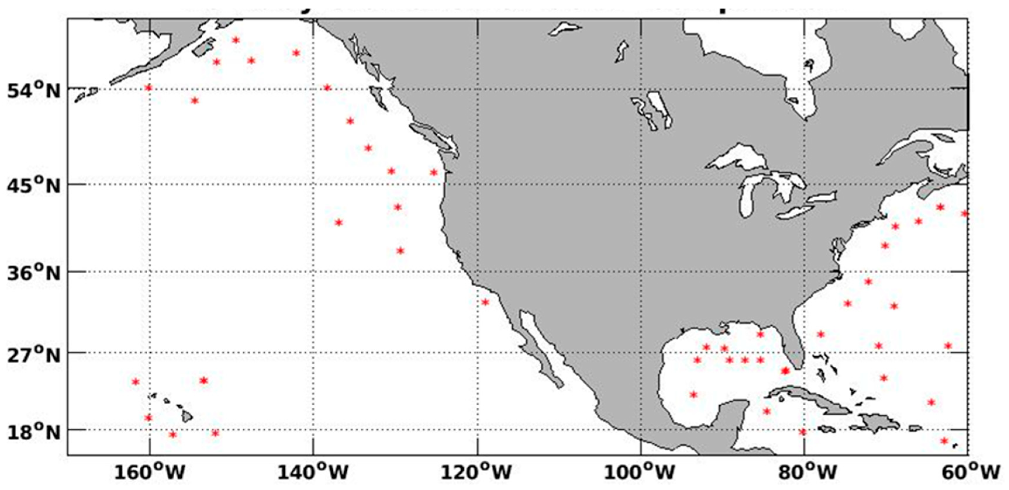
Wind measurements from 48 buoy stations around the continental U.S. and Hawaii islands, available from National Data Buoy Center, were used in our evaluation. The location, station ID, and number of records are listed in the supplementary material of the paper. These stations operated over different periods. The number of stations available for comparison varies from 22 to 38, with a median value of 29 stations for each month. Figure 1 shows the location of these 48 stations. Before the comparison, the buoy winds were adjusted to 10 m height under the neutral stability assumption following the method described in the supplementary material of Atlas et al. [1]. The method is explained in Equations (1) and (2) below, and the height of buoy stations was assumed to be 3.4 m unless specifically stated otherwise. The CCMP winds were interpolated to buoy locations. Temporal interpolation was also conducted from 6 hourly CCMP products to match the times of the buoy wind observations. Our comparison period was from 2000 to 2018. The total record number for comparison was over 7 × 10⁵.
2.3. Wind Power Density Computation
To analyze the wind power density at 100 m height, the 10 m wind from CCMP was extrapolated to 100 m using a logarithmic relation following the method explained in the supplementary material of Atlas et al. [1]. The wind at height is
where are constants. For 10 m winds, the above equations are solved iteratively to compute and . Then, the winds at 100 m are computed. We solved the above equations for 10 m winds for a wind range of 0–100 m/s with 0.5 m/s interval to form a look-up table. The table was then used to estimate 100 m winds instead of solving the relation repeatedly. Equations (1) and (2) were also used to adjust buoy winds to 10 m height.
The wind power density P was estimated using the method from Liu et al. [7], assuming a Weibull distribution of wind speed,
where is air density (taken as a constant 1.29 kg/m3 as in other wind power literature). C and k are computed as
and and are the mean and standard deviation of wind speed, respectively. is the Gamma function. Different wind speed distributions were tested, and the results show that the Weibull distribution is not necessarily the best fit for all the locations; the wind power density estimation would change when different wind speed distributions were used [23,24]. Thus, the wind power density was also directly estimated using wind speed at each time following the formula below.
The differences between the wind power density using wind speed directly and using a Weibull distribution for 48 buoy stations was within 2% for 100 m height. In our analysis, we used Equation (3) for the estimation of wind power density.
3. Results
3.1. Difference between CCMP3.0 and CCMP2.0
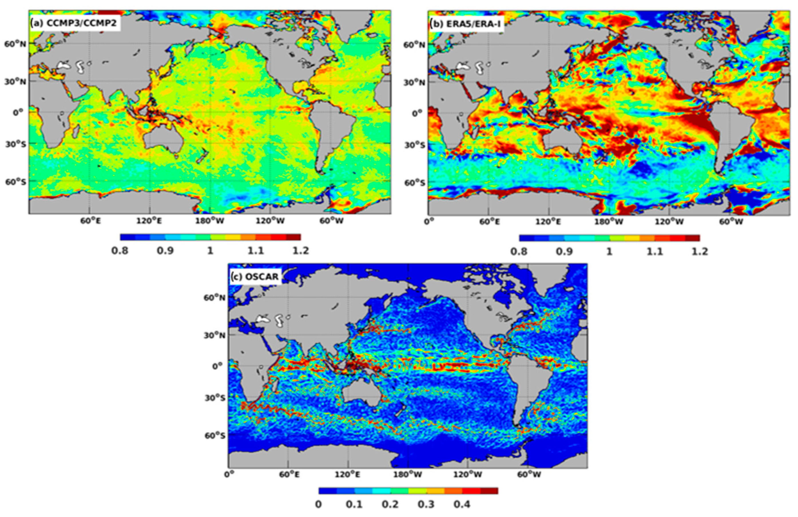
We randomly chose two months to analyze the difference between CCMP3.0 and CCMP2.0. For January 2000, Figure 2 presents the ratio of the CCMP3.0 and CCMP2.0 monthly mean wind speed, the ratio of respective background ERA5 neutral wind speed, ERA-Interim wind speed, and the monthly averaged OSCAR current. The winds from CCMP3.0 and CCMP2.0 agree well with the ratio of wind speed varying around 1 (Figure 2a). The ratio of the respective background wind fields (i.e., between 10 m neutral winds from ERA5 and 10 m winds from ERA-Interim) deviated substantially from 1 in many regions (Figure 2b). This indicates that the satellite observations make the CCMP3.0 and CCMP2.0 winds more consistent with each other, and the background fields play a minor role in locations where satellite wind observations are available. Some regional differences between CCMP3.0 and CCMP2.0 might be related to the ocean currents, especially those around the Gulf Stream extension in the Atlantic Ocean. The difference between CCMP3.0 and CCMP2.0 in the tropical region may come from a combination of background field differences and the effect of ocean current adjustment in CCMP3.0 (e.g., the difference in the eastern equatorial Pacific where ocean currents are strong). The difference in CCMP3.0 and CCMP2.0 in the South Pacific Convergence Zone might be mainly caused by the difference in their respective background fields. The same is true at high latitudes (e.g., around the Bering Strait and Antarctica).
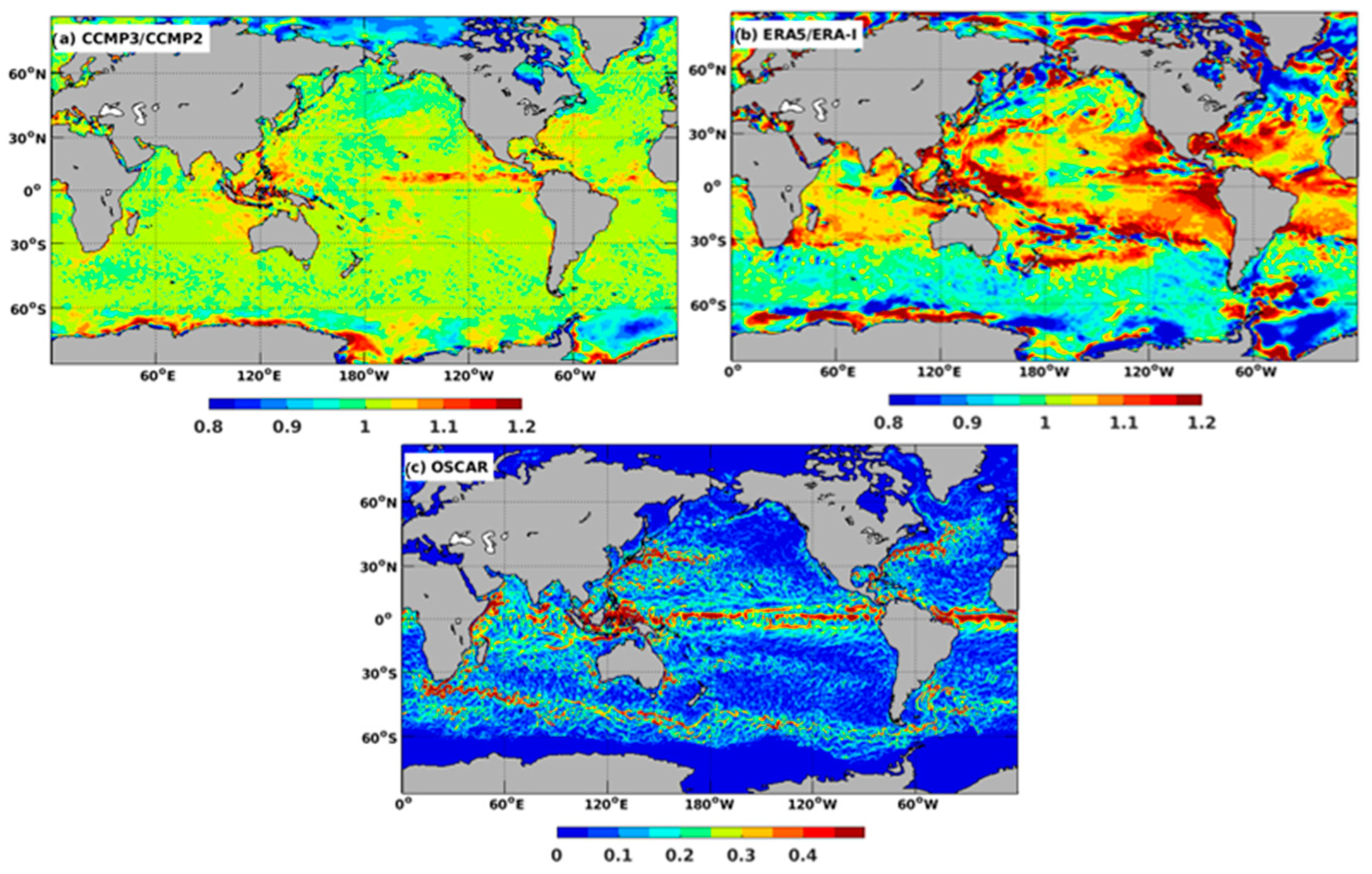
The ratio of CCMP3.0 and CCMP2.0 wind speed varied substantially from January 2000 to July 2000 at some locations, in part, due to atmospheric stability (Figure 3). The regions where the ratio of ERA5 neutral winds to ERA-Interim 10 m winds were greater than 1 shifted slightly to the northern hemisphere in July, presumably associated with the change in atmospheric stability. For the unstable regions, the 10 m neutral winds were larger than the 10 m winds. The difference between CCMP3.0 and CCMP2.0 in July in the tropical Pacific can be traced to the influence of ocean currents and atmospheric stability, as shown by the larger ratio between ERA5 neutral winds and ERA-Interim winds in these regions. The influence of the western boundary current, especially along the Gulf Stream extension, is still visible. The difference between CCMP3.0 and CCMP2.0 around the coastal region of Antarctica may come from the background fields, as was the case for January 2000. Statistically, the CCMP3.0 was improved compared with CCMP2.0, as demonstrated by Mears et al. [3]. For the differences between CCMP3.0 and CCMP2.0 at a specific time, the satellite wind observations, ocean currents, and background winds contributed differently for different regions.
3.2. Comparison of CCMP2.0/3.0 with Independent Buoy Wind
Table 2 summarizes the comparison of the CCMP wind speed with buoy observations. The statistics presented in the table are the average for all 48 stations. The number of comparison samples was set to at least 30 in computing the statistics. For buoy wind speeds higher than 15 m/s, the number of stations used in the average was 35 instead of 48 since some stations did not have more than 30 comparison samples. The correlation coefficients in Table 2 between buoy wind and CCMP (2.0 or 3.0) and between CCMP2.0 and CCMP3.0 were all significant at the 95% level. For all wind speed ranges, the correlation coefficients of CCMP2.0 vs. buoy and CCMP3.0 vs. buoy were the same. The root-mean-square-difference (RMSD) of CCMP2.0 vs. buoy wind speed (1.38 m/s) was slightly higher than that of CCMP3.0 vs. buoy (1.35 m/s). In contrast, the correlation coefficient of CCMP3.0 vs. CCMP2.0 (0.98) was much higher than that of CCMP2.0 vs. buoy and CCMP3.0 vs. buoy. The closeness of CCMP2.0 and CCMP3.0 was also shown by a small RMSD (0.62 m/s), about half of those between CCMP2.0 vs. buoy and CCMP3.0 vs. buoy.
The CCMP and buoy winds were also compared for high wind speed ranges. The comparison samples were selected based on the buoy wind speed. When the buoy wind speed was higher than 10 m/s, the RMSD of CCMP wind reduced slightly from CCMP2.0 (1.64 m/s) to CCMP3.0 (1.51 m/s), and the correlation coefficient increased from CCMP2.0 (0.71) to CCMP3.0 (0.76). The situation was similar for wind speeds higher than 15 m/s. For buoy wind speeds higher than 15 m/s, the correlation coefficient between buoy and CCMP2.0 was 0.55, which was much lower than that between CCMP3.0 and buoy (0.68). The RMSD of wind speeds reduced from 2.74 m/s between buoy and CCMP2.0 to 2.43 m/s between buoy and CCMP3.0. Overall, CCMP3.0 was closer to buoy observations at high wind speeds.
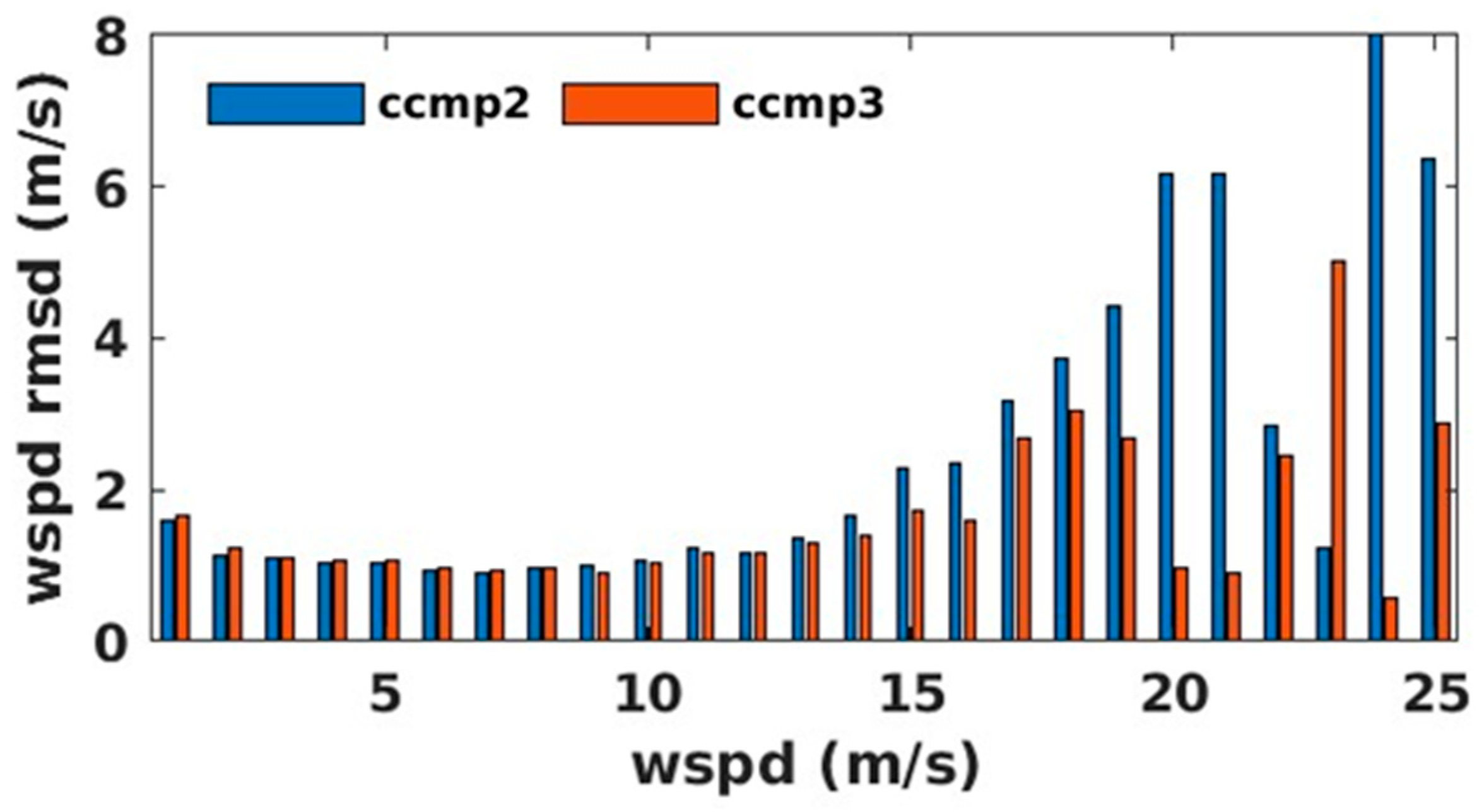
The RMSD of CCMP and buoy wind speed was also computed for different wind speed bins by combining data from all 48 stations. The buoy wind speed was separated into 25 bins with 1 m/s increments (i.e., 0–1 m/s, 1–2 m/s, etc., except the last wind speed bin, which was greater than 24 m/s). The RMSD of CCMP and buoy wind of the 25 bins are shown in Figure 4. When the wind speed was less than 12 m/s, the RMSDs of CCMP and buoy wind did not change much, with an average of around 1 m/s, 1.09 m/s for CCMP2.0, and 1.11 m/s for CCMP3.0. Starting from 12 m/s, the RMSD values for CCMP vs. buoy winds increase with the wind speed. The RMSD values of CCMP2.0 vs. buoy winds were consistently larger than those of CCMP3.0 vs. buoy winds. The large variability of RMSD values of both CCMP2.0 and CCMP3.0 vs. buoy winds at high wind speed bins may be caused by the limited number of comparison samples (hundreds for wind speeds higher than 20 m/s). In comparison, the number of comparison samples for wind speeds lower than 20 m/s was in the tens of thousands. Based on the comparison for different wind speed bins, the CCMP3.0 winds compared better with buoy winds when the wind speed was higher than 10–12 m/s. It is worth noting that the histogram adjustment used in CCMP3.0 caused an enhancement of wind speed frequency in CCMP3.0 from 9 to 14 m/s at these 48 stations, as shown in Figure S1 of the Supplementary material.
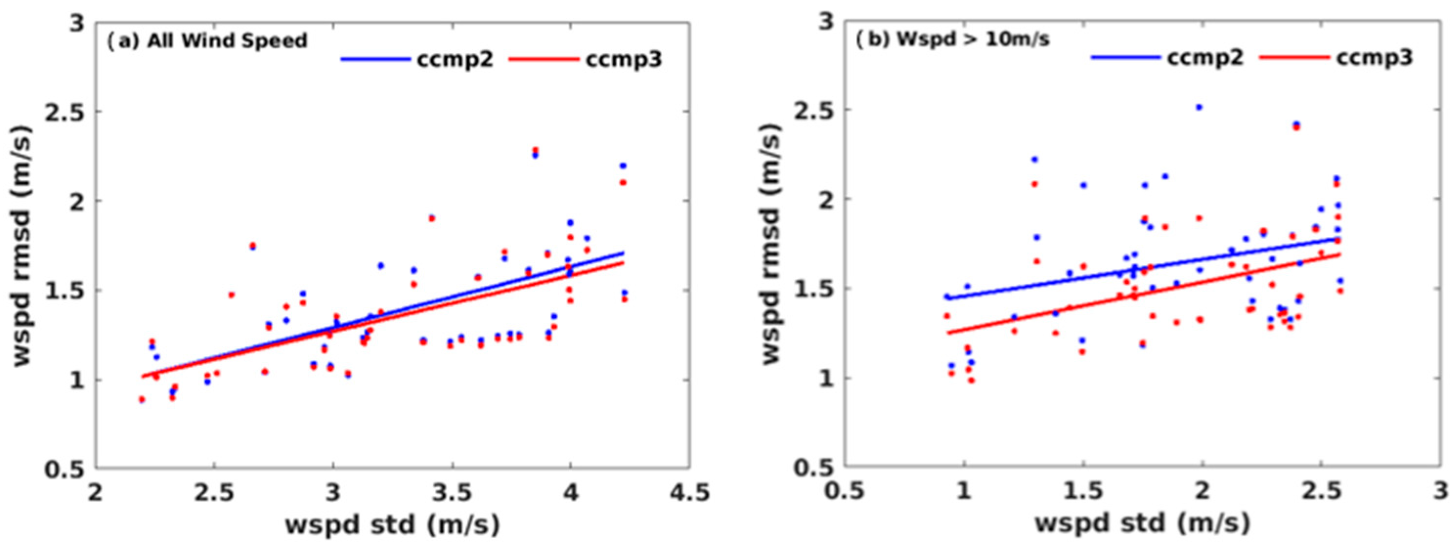
The better agreement of CCMP3.0 with buoy winds for high wind speeds occurred for almost all 48 stations. The standard deviation of buoy wind speed can be used to explain the variability of RMSD between CCMP and buoys among 48 stations (Figure 5). For all wind speed ranges, the correlation coefficient between RMSD and standard deviation of wind speed was 0.65 for CCMP2.0 and 0.62 for CCMP3.0, significant at the 95% confidence level. When the wind speed was greater than 10 m/s, the correlation coefficient between RMSD and standard deviation of wind speed was 0.31 for CCMP2.0 and 0.44 for CCMP3.0, also significant at the 95% confidence level (Table 3).
The change of wind speed RMSD with the standard deviation of buoy wind speed can be represented by a linear regression relation (Table 3). There was not much difference between the linear regression from CCMP2.0 and CCMP3.0 for all wind speed ranges (Figure 5a). When the wind speed was greater than 10 m/s, however, there was an obvious difference between the linear regression of CCMP2.0 and that of CCMP3.0, especially in terms of intercepts (Table 3, Figure 5b). As a result, the RMSD of CCMP2.0 was systematically higher than that of CCMP3.0 for wind speeds higher than 10 m/s based on the linear regression models. The correlation coefficient for the wind speed greater than 10 m/s was lower than that for all wind speeds (Table 3). There is more scatter in Figure 5b than in Figure 5a.
3.3. U.S. Coastal Wind Power Density Based on Different CCMP Wind Products
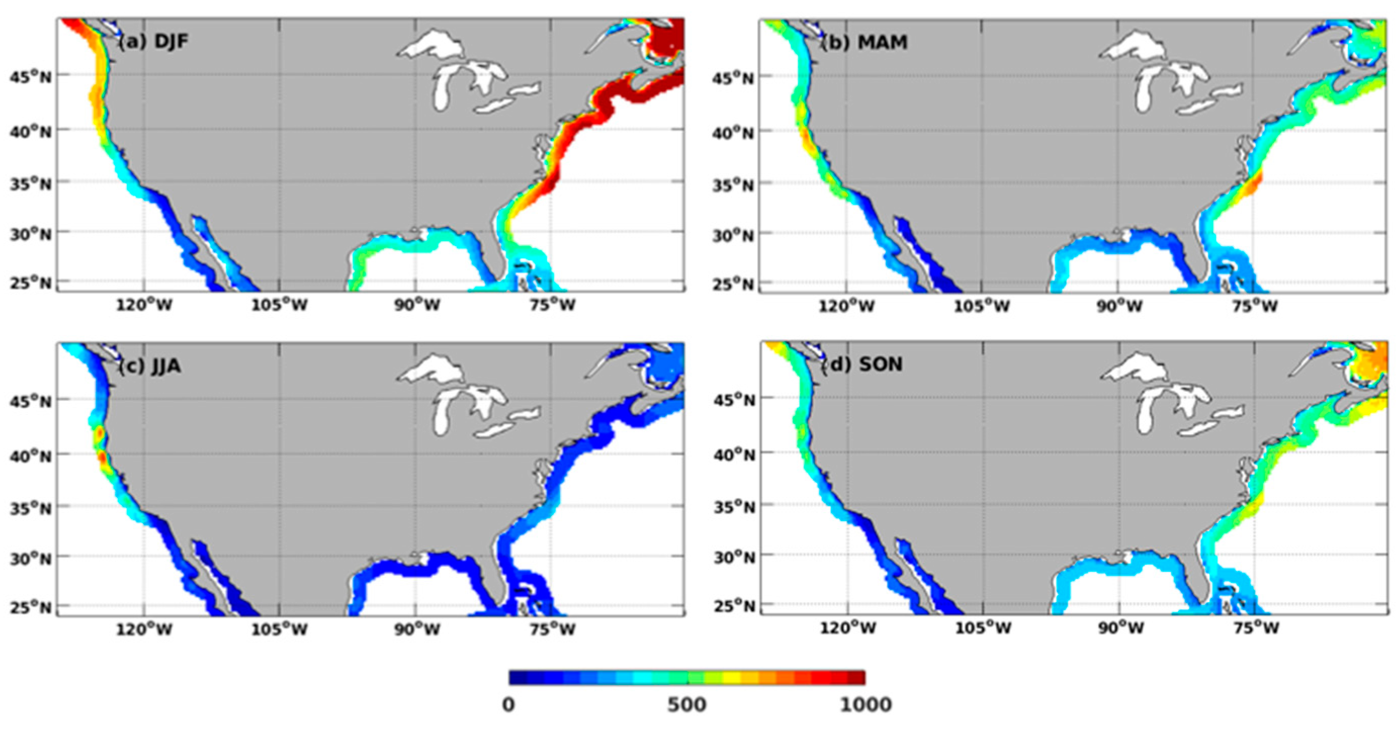
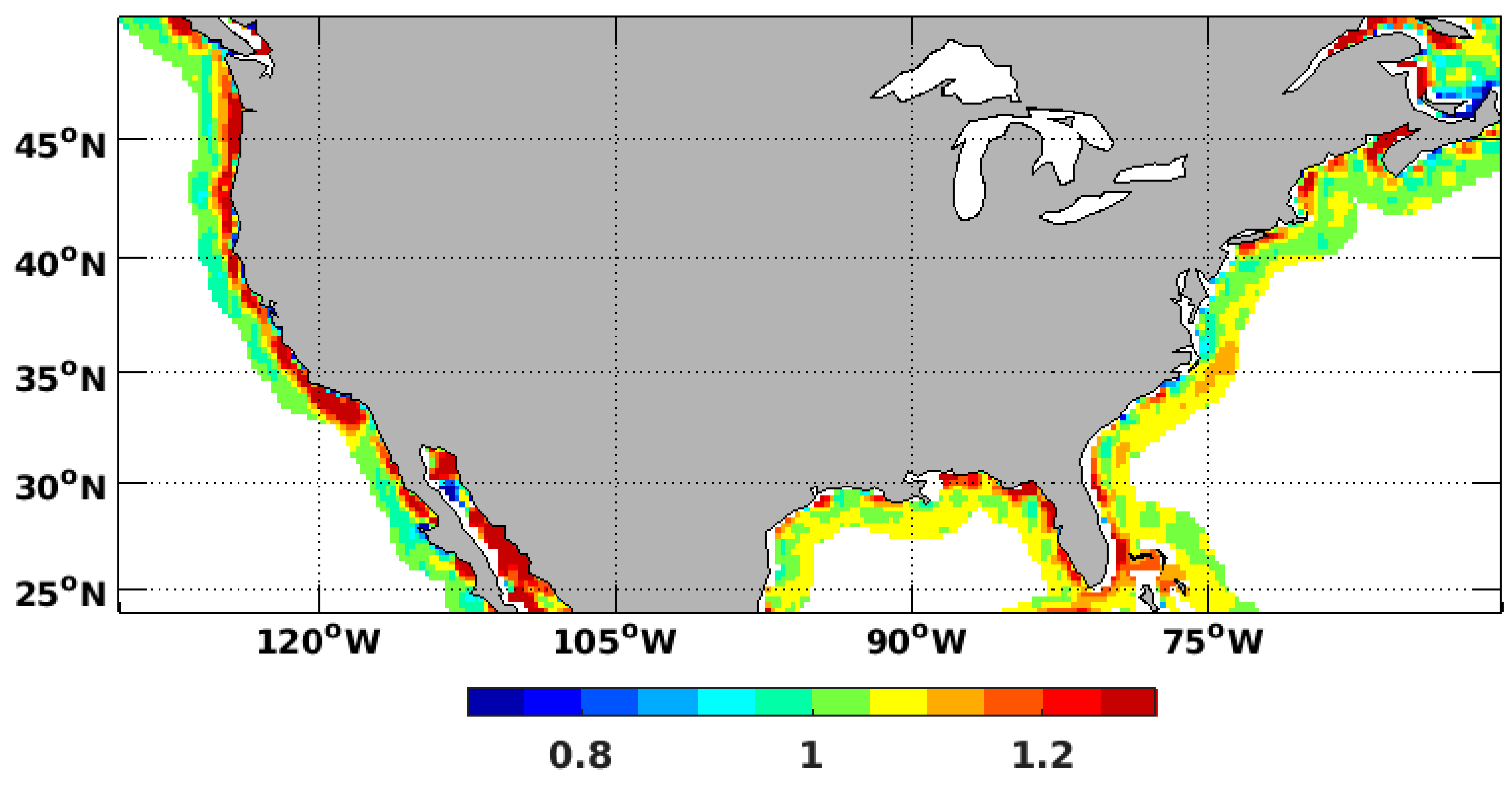
Since wind power density is related to the cube of mean wind speed, as shown in Equation (3), a subtle change in mean wind speed can cause a substantial change in wind power density. The averaged wind power density at 100 m height from 2000 to 2018 along the U.S. coast within 200 km for the potential development of wind power projects is presented in Figure 6. Both the eastern and western U.S. coastal regions have larger wind power density during winter (DJF) and spring (MAM), and the wind power density is at the lowest level during summertime (JJA), except for some particular regions along northern California and the Oregon coast. While there are marine environmental, coastal management, and logistic issues to consider when planning wind farm locations, the climatological wind power density distribution is one of the most important factors in the decision-making process. Compared with CCMP2.0, CCMP3.0 has a larger wind speed in coastal regions, which causes an increase in wind power density. The ratio of wind power density between CCMP3.0 and CCMP2.0 is generally larger than 1 along the U.S. coast (Figure 7). The enhancement of CCMP3.0 wind power density is greater along the U.S. western coastal region than the eastern coastal region. One interesting feature in Figure 7 is an enhanced ratio of wind power density between CCMP3.0 and CCMP2.0 along the coastal region, especially along the U.S. west coast, Gulf of Mexico, and Florida. Our analysis using the background field of CCMP3.0 and CCMP2.0 (Figure S2 in the Supplementary material) indicates that the enhancement associated with background fields disappears 50–100 km away from the coast in these regions. This indicates that the enhancement of the ratio along the coast is associated with the background fields, and the incorporation of satellite observations makes the two products more similar away from the coast. Overall, the wind speed at 100 m height of CCMP3.0 is increased by 1–2% compared with CCMP2.0 along the U.S. coastal region within 200 km. The standard deviation of wind speed of CCMP3.0 is increased by 3–5%. However, the wind power density along the U.S. coastal region is enhanced by 8–12% in CCMP3.0 for different seasons (Table 4).
3.4. Relationship of Wind Power Density with Climate Modes
Ocean surface winds are part of the climate system. How is wind power density related to climate variability? Currently, wind data are used in the planning, building, and operational stages of wind farms. During the operational stage, the wind forecast is used to predict wind power at different time scales, typically from several hours to one day, to balance the electricity grid. There is also a need for wind power predictions at longer time scales for potential wind power management, such as subseasonal to interannual time scales since both the usage and generation of renewable power would vary greatly. Thus, we also analyze the relationship of wind power density along the U.S. coastal region with the indices of major climate modes, such as the AMO (Atlantic Multi-decadal Oscillation), AO (Arctic Oscillation), NAO (North Atlantic Oscillation), Niño3.4, and PDO (Pacific Decadal Oscillation).
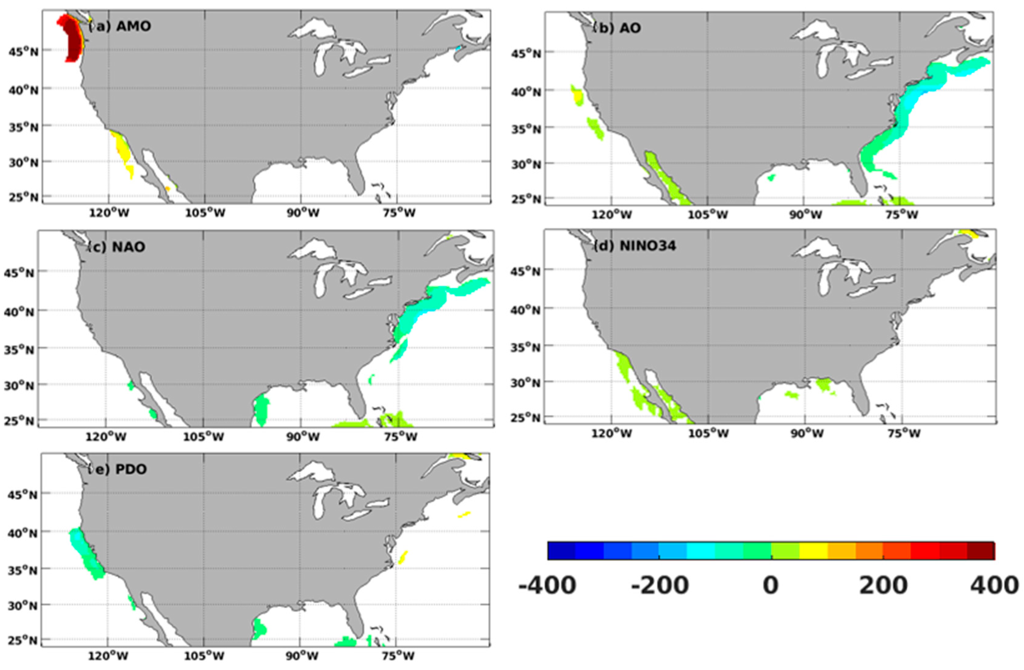
These climate indices are associated with large-scale circulation pattern anomalies. Some of them, such as Niño3.4, are also predicted routinely by the operational forecast community. Their potential to predict wind power generation needs to be explored. As a first step, linear regression models are built between these climate indices (original) and the anomaly of monthly wind power density at a 100 m height. Figure 8 shows the linear regression coefficient of wind power density and climate indices, i.e., the change of wind power density associated with one unit change of the respective climate indices to compare the relative influence of these indices to wind power density. Only the regions that have a significant correlation coefficient at the 95% confidence level are shown in Figure 8. From Figure 8, AMO is associated with wind power density change in the coastal region of Washington State and the Southern California coast. The AO, on the other hand, is associated with wind power density change along the California coast and a broad region of the U.S. eastern coast, which is not surprising since AO is associated with large-scale general circulation changes in the midlatitudes of the Northern Hemisphere. When the AO index is positive, both the Aleutian Low and Iceland Low are enhanced, which is associated with a strengthening of westerly winds south of the low-pressure centers. Like the spatial pattern associated with the AO index, the NAO index is mainly associated with wind power density changes along the U.S. eastern coast. Niño3.4 and PDO indices are associated with wind power density changes along the U.S. western coastal region, especially the California coastal region. More sophisticated methods could be explored to predict wind power density at longer time scales for specific wind farm locations.
4. Conclusions
The difference between CCMP2.0 and CCMP3.0 is primarily at high winds, as shown using the difference between independent buoy winds and the two CCMP products. The differences between CCMP3.0 and buoy winds are slightly reduced, especially for winds higher than 10 m/s. Using CCMP3.0, the wind power density along the coastal region is enhanced by 8–12%. Some commonly used climate indices have a significant correlation with wind power density along the U.S. coastal region. Wind power density along the U.S. eastern coastal region is associated with NAO; along the U.S. western coastal region, it is associated with Niño3.4, PDO, and AMO. The wind power density changes along both the eastern and western coasts is also associated with AO. The relationship between wind power density and major climate mode indices could be further explored to predict wind power generation at subseasonal to interannual time scales.
Supplementary Materials
The following supporting information can be downloaded at: https://www.mdpi.com/article/10.3390/rs15102620/s1, Table S1: The details of the 48 stations used for CCMP2.0 and CCMP3.0 product validation. Figure S1: The averaged difference of histograms at 48 stations before and after the wind speed histogram adjustment. Figure S2: Ratio of winter (DJF) wind power density for 100 m computed by using EAR5 10 m neutral wind (background for CCMP3.0) and ERA-Interim 10 m wind (background for CCMP2.0).
Author Contributions
Conceptualization, T.L., X.W. and C.M.; methodology, X.W.; software, X.W.; formal analysis, X.W.; resources, T.L.; data curation, C.M.; writing—original draft preparation, X.W.; writing—review and editing, X.W., T.L. and C.M.; project administration, T.L.; funding acquisition, T.L. All authors have read and agreed to the published version of the manuscript.
Funding
This research was funded under the Ocean Vector Wind Science Team of the National Aeronautics and Space Administration (NASA). The research was carried out in part at the Jet Propulsion Laboratory, California Institute of Technology, under a contract with NASA (80NM0018D0004). © 2023. All rights reserved.
Data Availability Statement
The CCMP2.0 and CCMP3.0 data sets are available from Remote Sensing Systems https://www.remss.com (accessed on 1 June 2022).
Acknowledgments
The climate indices used in the present research are available from Climate Prediction Center, NOAA (https://cpc.ncep.noaa.gov, (accessed on 1 June 2022)). The buoy wind observations are from the National Data Buoy Center (https://www.ndbc.noaa.gov, (accessed on 1 June 2022)).
Conflicts of Interest
The authors declare no conflict of interest.
References
- Atlas, R.M.; Hoffman, R.N.; Ardizzone, J.; Leidner, S.M.; Jusem, J.C.; Smith, D.K.; Gombos, D. A Cross-Calibrated Multi-Platform Ocean Surface Wind Velocity Product for Meteorological and Oceanographic Applications. Bull. Am. Meteorol. Soc. 2011, 92, 157–174. [Google Scholar] [CrossRef]
- Mears, C.A.; Scott, J.; Wentz, F.J.; Ricciardulli, L.; Leidner, S.M.; Hoffman, R.; Atlas, R. A Near-Real-Time Version of the Cross-Calibrated Multiplatform (CCMP) Ocean Surface Wind Velocity Data Set. J. Geophys. Res. Ocean 2019, 124, 6997–7010. [Google Scholar] [CrossRef]
- Mears, C.; Lee, T.; Ricciardulli, L.; Wang, X.; Wentz, F. Improving the Accuracy of the Cross-Calibrated Multi-Platform (CCMP) Ocean Vector Winds. Remote Sens. 2022, 14, 4230. [Google Scholar] [CrossRef]
- Dee, D.P.; Uppala, S.M.; Simmons, A.J.; Berrisford, P.; Poli, P.; Kobayashi, S.; Andrae, U.; Balmaseda, M.A.; Balsamo, G.; Bauer, P.; et al. The ERA-Interim Reanalysis: Configuration and Performance of the Data Assimilation System. Q. J. R. Meteorol. Soc. 2011, 137, 553–597. [Google Scholar] [CrossRef]
- McGregor, S.; Sen Gupta, A.; Dommenget, D.; Lee, T.; McPhaden, M.J.; Kessler, W.S. Factors Influencing the Skill of Synthesized Satellite Wind Products in the Tropical Pacific. J. Geophys. Res. Ocean 2017, 122, 1072–1089. [Google Scholar] [CrossRef]
- Hersbach, H.; Bell, B.; Berrisford, P.; Hirahara, S.; Horányi, A.; Muñoz-Sabater, J.; Nicolas, J.; Peubey, C.; Radu, R.; Schepers, D.; et al. The ERA5 Global Reanalysis. Q. J. R. Meteorol. Soc. 2020, 146, 1999–2049. [Google Scholar] [CrossRef]
- Liu, W.T.; Tang, W.; Xie, X. Wind power distribution over the ocean. Geophys. Res. Lett. 2008, 35, L13808. [Google Scholar] [CrossRef]
- Guo, Q.; Xu, X.; Zhang, K.; Li, Z.; Huang, W.; Mansaray, L.R.; Liu, W.; Wang, X.; Gao, J.; Huang, J. Assessing Global Ocean Wind Energy Resources Using Multiple Satellite Data. Remote Sens. 2018, 10, 100. [Google Scholar] [CrossRef]
- Waewsak, J.; Landry, M.; Gagnon, Y. Offshore wind power potential of the Gulf of Thailand. Renew. Energy 2015, 81, 609–626. [Google Scholar] [CrossRef]
- Sherman, P.; Chen, X.; McElroy, M.B. Wind-generated Electricity in China: Decreasing Potential, Interannual Variability and Association with Changing Climate. Nat. Sci. Rep. 2017, 7, 16294. [Google Scholar] [CrossRef] [PubMed]
- He, J.; Chan, P.W.; Li, Q.; Lee, C.W. Spatiotemporal analysis of offshore wind field characteristics and energy potential in Hong Kong. Energy 2020, 201, 117622. [Google Scholar] [CrossRef]
- Costoya, X.; deCastro, C.M.; Carvalho, M. Gomez-Gesteira, On the suitability of offshore wind energy resource in the United States of America for the 21st century. Appl. Energy 2020, 262, 115347. [Google Scholar] [CrossRef]
- Kumar, V.S.; Asok, A.B.; George, J.; Amrutha, M.M. Regional Study of Changes in Wind Power in the Indian Shelf Seas over the Last 40 Years. Energies 2020, 13, 2295. [Google Scholar] [CrossRef]
- de Assis Tavares, L.F.; Shadman, M.; de Freitas Assad, L.P.; Silva, C.; Landau, L.; Estefen, S.F. Assessment of the offshore wind technical potential for the Brazilian Southeast and South regions. Energy 2020, 196, 117097. [Google Scholar] [CrossRef]
- Wang, Y.-H.; Walter, R.K.; White, C.; Farr, H.; Ruttenberg, B.I. Assessment of surface wind datasets for estimating offshore wind energy along the Central California Coast. Renew. Energy 2019, 133, 343–353. [Google Scholar] [CrossRef]
- NREL (National Renewable Energy Laboratory) Renewable Energy Supply Curves. 2022. Available online: https://www.nrel.gov/gis/renewable-energy-supply-curves.html (accessed on 1 June 2022).
- Diaz, H.; Guedes Soares, E. An integrated GIS approach for site selection of floating offshore wind farms in the Atlantic continental European coastline. Renew. Sustain. Energy Rev. 2020, 134, 110328. [Google Scholar] [CrossRef]
- Denholm, P.; Patrick, B.; Wesley, C.; Trieu, M.; Brianet, S.; Maxwell, B.; Jaige, J.; Jonathan, H.; Jack, M.; Colin, M.; et al. Examining Supply-Side Options to Achieve 100% Clean Electricity by 2035; National Renewable Energy Laboratory: Golden, CO, USA, 2022. Available online: https://www.nrel.gov/docs/fy22osti/81644.pdf (accessed on 7 February 2023).
- The White House. Fact Sheet: President Biden Sets 2030 Greenhouse Gas Pollution Reduction Target Aimed at Creating Good-Paying Union Jobs and Securing, U.S. Leadership on Clean Energy Technologies. 2021. Available online: https://www.whitehouse.gov/briefing-room/statementsreleases/2021/04/22/fact-sheet-president-biden-sets-2030-greenhouse-gas-pollution-reductiontarget-aimed-at-creating-good-paying-union-jobs-and-securing-u-s-leadership-on-clean-energytechnologies/ (accessed on 22 April 2022).
- Walter, M.; Spitsen, P.; Beiter, P.; Duffy, P.; Marquis, M.; Cooperman, A.; Hammond, R.; Shields, M. Offshore Wind Market Report: 2021 Edition; National Renewable Energy Laboratory: Golden, CO, USA, 2021. Available online: https://www.energy.gov/sites/default/files/2021-08/Offshore%20Wind%20Market%20Report%202021%20Edition_Final.pdf (accessed on 7 February 2023).
- Bonjean, F.; Lagerloef, G.S.E. Diagnostic Model and Analysis of the Surface Currents in the Tropical Pacific Ocean. J. Phys. Oceanogr. 2002, 32, 2938–2954. [Google Scholar] [CrossRef]
- Dohan, K. Ocean surface currents from satellite data. J. Geophys. Res. Ocean. 2017, 122, 2647–2651. [Google Scholar] [CrossRef]
- Morgan, E.C.M.; Lackner, M.; Vogel, R.M.; Baise, L.G. Probability distributions for offshore wind speeds. Energy Convers. Manag. 2011, 52, 15–26. [Google Scholar] [CrossRef]
- Soukissian, T. Use of multi-parameter distributions for offshore wind speed modeling: The Johnson SB distribution. Appl. Energy 2013, 111, 982–1000. [Google Scholar] [CrossRef]
Figure 1.
The 48 independent buoy stations (indicated by red stars) around the U.S. where the in situ wind data were used to evaluate CCMP3.0 product.
Figure 1.
The 48 independent buoy stations (indicated by red stars) around the U.S. where the in situ wind data were used to evaluate CCMP3.0 product.

Figure 2.
(a)Ratio of CCMP3.0 and CCMP2.0 wind speed, (b) ratio of ERA5 and ERA-Interim wind speed, and (c) averaged OSCAR current of Jan 2000.
Figure 2.
(a)Ratio of CCMP3.0 and CCMP2.0 wind speed, (b) ratio of ERA5 and ERA-Interim wind speed, and (c) averaged OSCAR current of Jan 2000.

Figure 3.
(a) Ratio of CCMP3.0 and CCMP2.0 wind speed, (b) ratio of ERA5 and ERA-Interim wind speed, and (c) averaged OSCAR ocean current of July 2000.
Figure 3.
(a) Ratio of CCMP3.0 and CCMP2.0 wind speed, (b) ratio of ERA5 and ERA-Interim wind speed, and (c) averaged OSCAR ocean current of July 2000.

Figure 4.
Root-mean-square difference (RMSD) of CCMP and buoy winds for different buoy wind speed bins.
Figure 4.
Root-mean-square difference (RMSD) of CCMP and buoy winds for different buoy wind speed bins.

Figure 5.
The relationship of root-mean-square-difference (RMSD) of CCMP, buoy wind, and wind speed standard deviation (STD). (a) For all wind speeds. (b) For wind speeds higher than 10 m/s.
Figure 5.
The relationship of root-mean-square-difference (RMSD) of CCMP, buoy wind, and wind speed standard deviation (STD). (a) For all wind speeds. (b) For wind speeds higher than 10 m/s.

Figure 6.
Averaged wind power density for different seasons from 2000 to 2018 for U.S. coastal regions within 200 km at 100 m height. (a) DJF, (b) MAM, (c) JJA, and (d) SON.
Figure 6.
Averaged wind power density for different seasons from 2000 to 2018 for U.S. coastal regions within 200 km at 100 m height. (a) DJF, (b) MAM, (c) JJA, and (d) SON.

Figure 7.
Ratio of averaged winter (DJF) wind power density at 100 m height based on CCMP3.0 and CCMP2.0 for U.S. coastal region.
Figure 7.
Ratio of averaged winter (DJF) wind power density at 100 m height based on CCMP3.0 and CCMP2.0 for U.S. coastal region.

Figure 8.
Linear regression coefficient of wind power density against climate indices, (a) AMO, (b) AO, (c) NAO, (d) Niño3.4, and (e) PDO.
Figure 8.
Linear regression coefficient of wind power density against climate indices, (a) AMO, (b) AO, (c) NAO, (d) Niño3.4, and (e) PDO.


Table 1.
Three major adjustments in CCMP3.0 compared with CCMP2.0.
| CCMP2.0 | CCMP3.0 |
|---|---|
| ERA-Interim 10 m wind as background | ERA5 10 m neutral winds as background |
| Not Applied | Wind speed histogram adjustment |
| Not Applied | Surface current is removed |
Table 2.
The average correlation coefficient and root-mean-square-difference (RMSD) between CCMP and buoy wind speed of 48 stations for different buoy wind speed ranges. For the situation when the wind speed was greater than 15 m/s, the average of 35 stations was used since some stations did not have more than 30 comparison samples.
| Corr Coef RMSD (m/s) | Buoy vs. CCMP2.0 | Buoy vs. CCMP3.0 | CCMP2.0 vs. CCMP3.0 | |
|---|---|---|---|---|
| All wind speed range | Corr Coef | 0.91 | 0.91 | 0.98 |
| RMSD | 1.38 | 1.35 | 0.62 | |
| Corr Coef | 0.71 | 0.76 | 0.91 | |
| RMSD | 1.64 | 1.51 | 0.77 | |
| Corr Coef | 0.55 | 0.68 | 0.83 | |
| RMSD | 2.74 | 2.43 | 1.42 |
Table 3.
The intercepts and coefficients of linear regressions between the RMSD of CCMP and buoy wind speed and standard deviation of wind speed for 48 buoy stations. The correlation coefficient between RMSD and standard deviation of wind speed is also shown in the last column. All the correlation coefficients are significant at 95% level.
| Product | Intercept | Coef | Corr. Coef | |
|---|---|---|---|---|
| All wind speed range | CCMP2 | 0.2785 | 0.3407 | 0.65 |
| CCMP3 | 0.3285 | 0.3135 | 0.62 | |
| CCMP2 | 1.2500 | 0.2057 | 0.31 | |
| CCMP3 | 1.0000 | 0.2664 | 0.44 |
Table 4.
The change of CCMP3.0 wind speed, wind speed standard deviation (STD), and wind power density along U.S. coast region relative to CCMP2.0 for different seasons (DJF, MAM, JJA, and SON).
Table 4.
The change of CCMP3.0 wind speed, wind speed standard deviation (STD), and wind power density along U.S. coast region relative to CCMP2.0 for different seasons (DJF, MAM, JJA, and SON).
| Wind Speed | Wind Speed STD | Wind Power Density | |
|---|---|---|---|
| DJF | 2.73% | 3.84% | 10.99% |
| MAM | 1.13% | 4.85% | 8.44% |
| JJA | 1.41% | 5.29% | 9.78% |
| SON | 2.67% | 4.97% | 12.04% |
Disclaimer/Publisher’s Note: The statements, opinions and data contained in all publications are solely those of the individual author(s) and contributor(s) and not of MDPI and/or the editor(s). MDPI and/or the editor(s) disclaim responsibility for any injury to people or property resulting from any ideas, methods, instructions or products referred to in the content. |
© 2023 by the authors. Licensee MDPI, Basel, Switzerland. This article is an open access article distributed under the terms and conditions of the Creative Commons Attribution (CC BY) license (https://creativecommons.org/licenses/by/4.0/).
Share and Cite
MDPI and ACS Style
Wang, X.; Lee, T.; Mears, C. Evaluation of Blended Wind Products and Their Implications for Offshore Wind Power Estimation. Remote Sens. 2023, 15, 2620. https://doi.org/10.3390/rs15102620
AMA Style
Wang X, Lee T, Mears C. Evaluation of Blended Wind Products and Their Implications for Offshore Wind Power Estimation. Remote Sensing. 2023; 15(10):2620. https://doi.org/10.3390/rs15102620
Chicago/Turabian StyleWang, Xiaochun, Tong Lee, and Carl Mears. 2023. "Evaluation of Blended Wind Products and Their Implications for Offshore Wind Power Estimation" Remote Sensing 15, no. 10: 2620. https://doi.org/10.3390/rs15102620
Note that from the first issue of 2016, this journal uses article numbers instead of page numbers. See further details here.