Case Study of a Mesospheric Temperature Inversion over Maïdo Observatory through a Multi-Instrumental Observation

Abstract

The dynamic vertical coupling in the middle and lower thermosphere (MLT) is documented over the Maïdo observatory at La Réunion island (21°S, 55°E). The investigation uses data obtained in the framework of the Atmospheric dynamics Research InfraStructure in Europe (ARISE) project. In particular, Rayleigh lidar and nightglow measurements combined with other observations and modeling provide information on a mesospheric inversion layer (MIL) and the related gravity waves (GWs) on 9 and 10 October 2017. A Rossby wave breaking (RWB) produced instabilities in the sheared background wind and a strong tropospheric activity of GWs on 9–11 October above La Réunion. The MIL was observed on the night of 9 October when a large amount of tropospheric GWs propagated upward into the middle atmosphere and disappeared on 11 October when the stratospheric zonal wind filtering became a significant blocking. Among other results, dominant mesospheric GW modes with vertical wavelengths of about 4–6 km and 10–13 km can be traced down to the troposphere and up to the mesopause. Dominant GWs with a wavelength of ~2–3 km and 6 km also propagated upward and eastward from the tropospheric source into the stratosphere on 9–11 October. Sounding of the Atmosphere using Broadband Emission Radiometry (SABER) temperature and OH profiles indicate that GW activity in the middle atmosphere affects the upper atmosphere with waves breaking at heights below the MIL and in the mesopause. Several techniques are illustrated on nightglow images to access GW activity and spectral characteristics at the mesopause for high and low frequency GWs on the nights of 9–10 October. In conclusion, intense tropospheric activity of GWs induced by RWB events can be linked with MILs at the subtropical barrier in the South-West Indian Ocean during austral winter.

1. Introduction

The region comprising the mesosphere and the lower thermosphere (MLT, located between 50 and 150 km), remains the least known of the atmosphere, due to a lack of observations and knowledge of vertical dynamic coupling [1]. Our current knowledge of stratosphere-troposphere coupling processes and fine-scale numerical modeling in the lower atmosphere allows the inclusion of the stratosphere in meteorological models, thereby improving the Brewer–Dobson circulation, winds near the tropopause, the representation of the quasi-biennial oscillation (QBO) in the equatorial region [2,3,4,5,6]. Surface weather forecasting at different time scales is also progressing thanks to troposphere-stratosphere wave connections [7].

Realistic representations of small-scale GWs remain a real challenge for the modeling of the general circulation and the climate. These ubiquitous atmospheric structures are mainly generated in the troposphere from sources such as deep convection, tropical cyclones, atmospheric jet, orography, atmospheric front, volcanic eruption, etc. Their periods of oscillation vary from a few minutes to 3–4 days for horizontal wavelengths between 10 km and several thousand kilometers, and vertical wavelengths from 1 km to 40–50 km. They can significantly affect the background atmosphere during their vertical propagation towards the upper atmosphere. The eruption of the Tonga volcano in January 2022, for example, recently produced impressive GWs observed in the different atmospheric layers [8].

Along with planetary and tidal waves, GWs play an important role in atmospheric processes in the upper atmosphere. Indeed, the amplitudes of GWs increase considerably with the decrease in atmospheric density with altitude in the absence of dissipation. A small amount of energy from tropospheric GWs can therefore become significant in the upper atmosphere [9,10]. Numerical simulations show that the dissipation of GWs could warm the thermosphere by several tens of kelvins per day with a downward cooling of 12–18% [11]. In addition to solar energy, GWs as well as Rossby and tidal waves are sources of variability in conductivities in the E region (90–120 km) that modulate thermospheric temperature, wind structure and ionospheric electrodynamics. They also indicate that the propagation of GWs disturbs the balance of gaseous constituents in the mesosphere and the thermosphere. Observations reveal that GWs are also of varied natures in the MLT, presenting horizontal wavelengths ranging from 24 to 4000 km, and vertical from 17 to 30 km and intrinsic periods from 10 min to 12 h [12]. The climate model WACCM (Whole Atmosphere Community Climate Model) made it possible to reproduce the propagation of GWs generated by a tropical cyclone up to the upper atmosphere [13]. Estimates of energy fluxes in the upper atmosphere from GWs are comparable to those of shortwave solar radiation fluxes that control the temperature of the upper atmosphere. The non-linear interactions of GWs are also sources of secondary GWs at the origin of great disturbances of the thermosphere and the ionosphere [14]. The middle atmosphere, the intermediate layer between the lower atmosphere and the upper atmosphere, is a key region for atmospheric processes in the upper atmosphere. Indeed, most global climate models currently lower their lower limit to the stratosphere. If the atmospheric processes of the stratospheric circulation are better represented, the advances evolve little in the upper part of the middle atmosphere, a region dynamically very active for wave structures [15]. In this context, the European project ARISE (Atmospheric dynamics Research InfraStructure in Europe, http://arise-project.eu/, accessed on 7 april 2023) has made it possible to build a collaborative European observation infrastructure to document, as a priority, the wave dynamic coupling between the stratosphere, the MLT and the thermosphere and in particular above the European continent.

The absence of vertical coupling with the troposphere in stratosphere–mesosphere modeling is notably responsible for the poor representation of mesospheric temperature inversions (MILs), which significantly disturb the mesosphere. These large-scale horizontal and persistent phenomena are suggested to arise due to various dynamics [16]. They are characterized by a minimum temperature with large deviations of several tens of Kelvins in the mesosphere with a strong positive lapse rate of the temperature above and a second maximum temperature [17]. However, several studies confirm that the breaking of GWs generates MILs [18,19,20]. At low and midlatitudes, MILs are characterized by a vertical extension of ~10 km region of enhanced temperatures (ΔT~15–50 K) in both the middle mesosphere (60–70 km) and the mesopause (90–100 km) [21]. The mechanisms and the strong interaction with GWs are currently attracting the interest of the scientific community for climate modeling [22,23]. They are linked with layers of wave turbulence which favor GW reflection instead of vertical transmission [16].

Statistical studies using lidar data from the Haute-Provence Observatory [17] in mid-latitudes and the Maïdo Observatory [24] show the ubiquity of MILs and the need to clarify the different processes involved. The variability of MILs above La Réunion is dominated by a semi-annual cycle with a maximum occurrence in late austral winter in October–November [24], as previously reported in [25] for tropical regions. In the northern tropics, amplitudes of MILs are revealed to be underestimated [26]; in particular, Ramesh et al. [27] identified three tropical MILs of different natures on the same night. The middle MIL at ~80 km was due to the turbulence generated by GW breaking. Singh and Pallamraju [28] suggested that both wave dynamics and chemical heating could work together for the occurrence of tropical upper MILs.

Simulations with the whole atmosphere-model WACCM correctly reproduce the main characteristics of MILs in the extratropical regions, but mainly in a statistical sense [29]. The improvement in the non-orographic GWs parameterization in forecasting models shows encouraging results on the dynamical process of the mesosphere, especially the semi-annual mesospheric oscillation (MSAO) in the tropical middle atmosphere. Indeed, small-scale GWs contribute significantly to the momentum budget of the MSAO during solstices [30] by the selective transmission of GWs through the stratospheric semi-annual oscillation (SSAO). However, general circulation models (GCMs) globally do not solve GWs very well and therefore call on various, more or less sophisticated and adjusted parameterizations. The uncertainties in the underlying physics, in the adjustment between the different GW parameterization schemes as well as in the actual location of the GW sources, lead to better constrained GCM models at their base by the meteorological forecasting models, which elsewhere have extended their upper altitudes to the middle atmosphere thanks to the assimilation of observations. Recent studies propose an alternative approach to the physics-based parameterization-based machine and deep learning [31,32,33] as a computationally cost-effective way for modeling. Nevertheless, the observations of each instrument only tell us about part of the GW spectrum, biasing the interpretation of the GWs observed in the different spectral ranges. The middle atmosphere also operates a constant filtering of GWs during their vertical propagation. For example, GWs that are not filtered by the stratospheric background wind, such as the QBO or the SSAO in the tropical atmosphere, can reach critical MSAO levels. A poor representation of the middle atmosphere therefore alters the wind filtering process and consequently the representation of the MLT. For example, the “hot-spots” of stratospheric GW activity over the mountainous islands of the Southern Ocean near 60°S during the austral winter are not included in GCM models, which are an important factor of the winter cold pole problem (“Cold-pole problem”) [34]. In conclusion, the study of the dynamical vertical coupling of the MLT by GWs is currently a priority for the international scientific community in order to improve GCM models of the upper atmosphere as well as connections between atmospheric layers in the different models [35].

Thus this present study describes a case study of MIL and the related GW process above the Maïdo observatory at La Réunion (21°S, 55°E) through a multi-instrumental observation near the southern subtropical barrier in austral winter 2017. The activity and characteristics of GWs as well as the wave coupling from the lower atmosphere to the lower thermosphere are investigated from both observations and modeling.

This paper is organized as follows: Section 2 introduces the data and methods for analyzing MILs and GWs, Section 3.1 documents a MIL as well as GW perturbations in the middle atmosphere during nights of 9 and 10 October 2017, Section 3.2 analyzes the source and the vertical propagation of GWs from the troposphere up to the middle atmosphere, Section 3.3 describes GW activity in the upper mesosphere and lower thermosphere and Section 4 gives a summary of the main results and conclusions.

2. Data and Analysis Methods

2.1. Data: Observations and Modeling

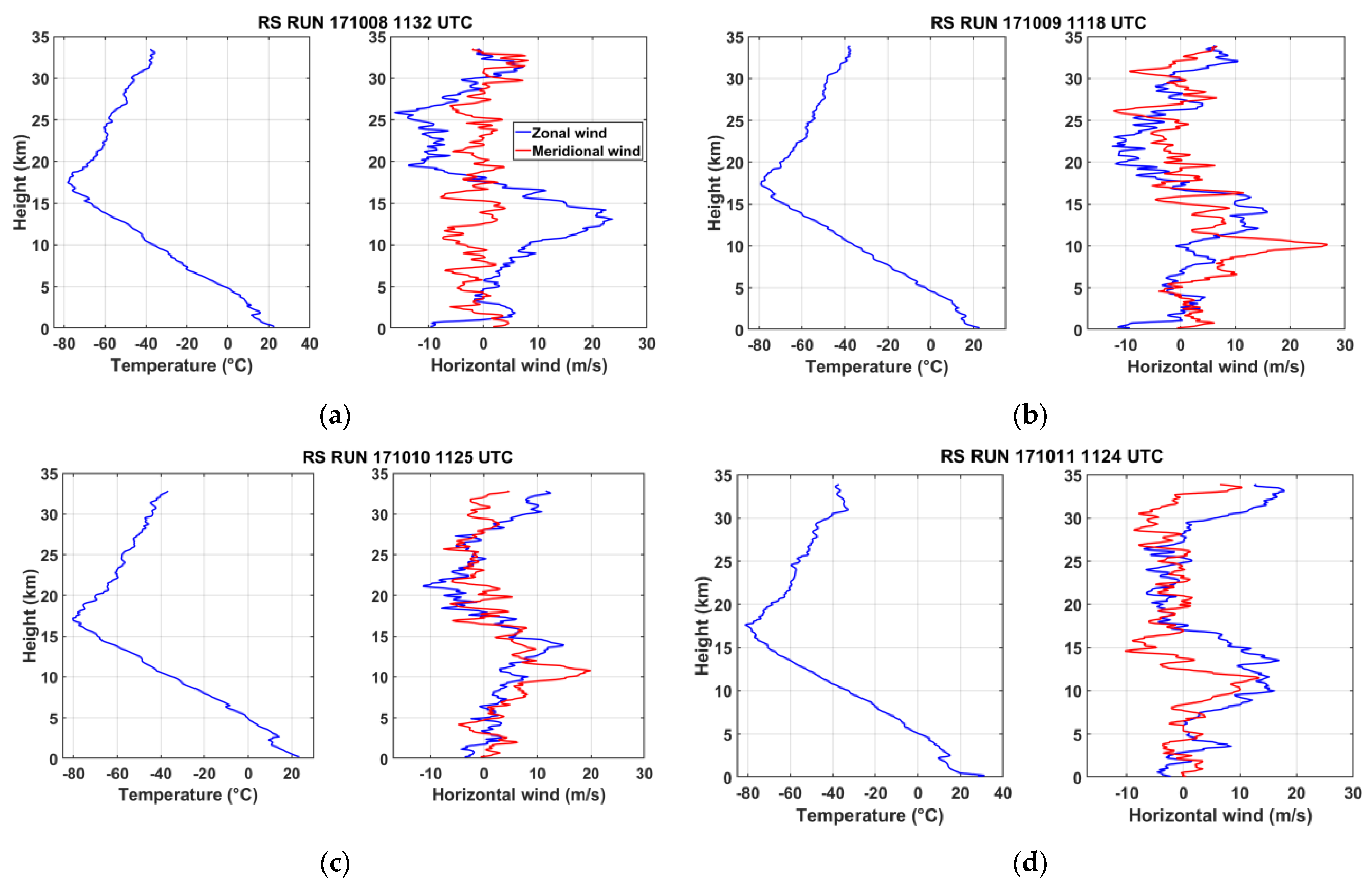
2.1.1. Radiosonde Data

Daily radiosonde measurements are collected at 1200 UTC by Meteo-France at Reunion Island since June 2011. Meteo-Modem M10 radiosondes were manually launched at Roland Garros airport (20.9°S, 55.5°E) until April 2018 when a Meteomodem robotsonde was located in the Regional Specialized Meteorological Center (RSMC). Profiles of temperature and horizontal wind have a vertical resolution <100 m at heights up to 32 km. Absolute accuracies are 0.3 °C, 0.15 m/s and 1° for temperature, horizontal wind speed and wind direction, respectively. Quality of temperature and wind measurements allow us to capture GW perturbations with vertical wavelengths of 1–15 km at heights <32 km above La Réunion [36]. Figure 1 visualizes 100 m resampled vertical profiles of temperature and horizontal wind on 8–11 October 2017 during the period of the study. During the winter season, tropospheric relative humidity is globally capped by the temperature inversion (Figure 1c,d), southeasterly trade winds are observed near the ground and the zonal wind of the subtropical jet peaks at about 20 m/s. In particular the subtropical jet is observed to be strongly perturbed on 9 and 10 October with a decrease in the zonal wind intensity towards 12–13 km altitude accompanied with a peak of the meridional wind intensity at 10 km altitude toward the north (Figure 1b,c).

In addition, large wind perturbations of GWs with vertical wavelength of about 2 km are clearly observed on the vertical profiles of meridional wind at heights of 11–20 km on 9 and 10 October.

2.1.2. Lidar Data

The Rayleigh-Mie-Raman (RMR) lidar, initially installed at the university of La Réunion, was upgraded when it was moved to the Maïdo Observatory [37] with a new telescope of 1.2 m diameter and a powerful laser. It provides vertical profiles of temperatures from 30 to 90 km and water vapor from the boundary layer to the lower stratosphere [38]. It belongs to the Network for Detection of Atmospheric Climate Change (NDACC) international network and has routinely operated twice a week during night-time since 2013. The Rayleigh lidar principle is based on the measurement of the atmospheric density, proportional to the molecular Rayleigh scattering, and the determination of the temperature by downward integration of the hydrostatic law [39]. The profile is initialized at the top assuming a seed temperature from the NRLMSISE-00 empirical atmospheric model [40]. The raw RMR temperature profiles are originally obtained with 1 min integration time and 150 m vertical resolution. Vertical smoothing and time binning are applied to improve the signal-to-noise ratio of the measurements depending on the scientific objectives. For nightly mean profiles available on the NDACC database a 2 km vertical smoothing is applied using a Hanning filter. The present study processes individual temperature profiles of 15 min integration time and 150 m vertical resolution to characterize GWs. Because of the time and vertical resolution, only GWs with vertical wavelengths of >1 km and observed periods of >1 h can be analyzed. A 5 min lag is used between two successive profiles of 9 and 10 October. The statistical uncertainty is computed from the photon counting noise that follows a Poisson statistical law [41]. For a night-time mean profile, temperature uncertainty is typically better than 1 K below a 60 km height, increasing to about 10 K at an 80 km height and 30 K at a 90 km height. GW characteristics are only estimated at heights < 70 km where the temperature uncertainty on the mean profile is <2 K.

2.1.3. Nightglow Data

A Short-Wave InfraRed (SWIR) camera based on a thermoelectrically cooled InGaAs detector (640 × 512 pixels, pitch 25 µm) was installed from June 2016 to April 2017 at the Maïdo observatory, providing nightglow image sequences every night. The spectral bandwidth of the camera ranges from 0.9 to 1.7 µm corresponding to the vibrational transitions ∆ν = 2 and 3 of the OH Meinel band system. Thus, the altitude of the observed layer is assumed to be around 87 km [42]. A 8 mm focal lens was mounted on the camera, leading to a field of view of 90° × 77°, involving a footprint of 170 km × 140 km at the OH layer altitude (~87 km) for a zenith observation. The camera is radiometrically calibrated in a low light level laboratory in Onera, allowing absolute integrated radiance measurements. The relative uncertainty of measurements is <20% and the integration time is 400 ms with a frame rate of 30 s. Then, the acquired raw nightglow images are radiometrically corrected (dark current, dome effect), unwarped to fix optical distortions and georeferenced to capture GW structures. Observed GW parameters such as horizontal wavelengths, phase speeds, and direction of horizontal propagation can be directly retrieved from nightglow images. Nightglow satellite data are also derived from the SABER instrument [43]. Onboard Thermosphere Ionosphere Mesosphere Energetics Dynamics (TIMED) platform, SABER uses a 10-channel broadband limb-scanning infrared radiometer covering the spectral range from 1.27 μm to 17 μm. The temperature uncertainty is about a few kelvins, increasing with height up to ± 5 K at an altitude of 110 km. Only GWs with horizontal and vertical wavelengths of >200 km and 5 km, respectively, can be fully observed within SABER OH (1.6 and 2.0 μm) and temperature profiles with a wide spatial averaging of about 300 km along the line-of-sight.

2.1.4. GROGRAT Model

The gravity-wave regional or global ray tracer (GROGRAT) model, was developed by the Naval Research Laboratory to trace GWs in the regional or global atmosphere up to the middle atmosphere [44,45]. The raytracing technique is based on the Wentzel–Kramers–Brillouin (WKB) approximation of which the conditions for the validity are reviewed in [46]. It mainly describes the evolution of GW amplitudes in a non-hydrostatic, rotating and stratified and compressible atmospheric medium in slow temporal evolution, forced by the temperature, wind and pressure or geopotential altitude background fields in the lower and middle atmosphere. The model is now widely used by the atmospheric research community to identify and validate GW sources, source spectra and GW effects along their propagation from the troposphere into the upper atmosphere in observations and models [47,48,49,50]. In particular this technique is very useful to produce a global climatology of GWs from satellite images, to test assumptions made in GW parameterization schemes and to overcome the observable parts of GW spectrum derived from instrumental observations [51]. In addition, new GW parameterization schemes based on GW raytracing are being developed to take account of the effects of GW vertical and horizontal propagation along the propagation as well as to reduce GW computation for numerical weather prediction models (NWP) and climate models [52,53].

2.1.5. Weather and Climate Models

The Atmospheric Research Whole Atmosphere Community Climate Model version 4 (WACCM4, https://www2.acom.ucar.edu/gcm/waccm, accessed on 11 April 2023) is a comprehensive GCM spanning the height range from the earth’s surface up to 150 km in the thermosphere and a key component of the National Center for Atmospheric Research (NCAR) Community Earth System Model version 1.0 (CESM1). The setups of the simulations used in our study are described in [54] with horizontal resolutions of 2.5° × 1.9° (144 × 96 grids) and 88 vertical levels included a nudging towards the Modern-Era Retrospective analysis for Research and Application version 2 (MERRA2) at a time step of 30 min. Dynamic output fields of temperature, horizontal wind and geopotential heights have a vertical resolution of <1.2 km in the troposphere and the lower stratosphere, between 1.2 km and 2 km up to 67 km height in the mesosphere and ~3 km in the lower thermosphere.

The fifth generation ECMWF reanalysis ERA5 [55] provides hourly estimates of atmospheric variables for the covered period 1950–present with horizontal resolutions of 0.25° × 0.25° and 137 vertical levels from the surface to the height of 80 km. The vertical resolution is ~250 m at heights of <20 km, between 500 and 700 m in the lower stratosphere (24–32 km) and between 1 and 2.5 km at heights of 37–70 km. At these resolutions, ERA5 is capable of resolving a broader spectrum of GWs in the troposphere and lower stratosphere with periods as short as 2 h. Lower limits of vertical and horizontal wavelengths are, respectively, 1–1.5 km and 60–70 km as shown in the southern midlatitudes and the tropics [56,57,58]. However, only GWs with horizontal wavelengths larger than 180 km (6 Δx) may be well resolved [59]. The Climate Data Store cloud server ensures fast access to post-processed ERA5 data on 37 pressure levels from 1000 to 1 hPa with high resolution in the lower stratosphere. Figure 2 compares the dynamic fields derived from WACCM and ERA5 datasets at ≈10.5 km height on 9 October 2017 at 1200 UTC above the South-West Indian Ocean (SWIO). Temperature and winds are consistent but better resolved for ERA5. The synoptic fields are characterized by a local heating in the temperature (Figure 2a,b), a split of the subtropical jet in the zonal wind (Figure 2c,d) and planetary waves in the meridional wind (Figure 2e,f) at the height level of the jet above La Réunion.

The Weather Research and Forecasting model (WRF) has become an international community mesoscale model for both atmospheric research and operational forecasting since its initial public release in 2000 [60,61]. Several studies have reported that the model is able to simulate realistic GWs with high, medium and low frequencies in comparison with observations [62,63]. The simulation of TC Soudelor (2015) near Taiwan shows that the model can produce high-resolution vertical profiles of horizontal wind and temperature with realistic GWs in comparison with radiosonde data [64].

2.1.6. Empirical Model of Horizontal Winds HWM14

HWM14 is an empirical model of the horizontal winds up to the upper thermosphere based on both satellite and ground-based data [65]. It provides a time-dependent, observationally based, global empirical specification of the upper atmospheric general circulation patterns and migrating tides. This allows the retrieval of GW intrinsic parameters, such as the direction of horizontal propagation source of the GWs as inputs for raytracing models [66,67]. In this study, high-altitude zonal and meridional winds are extracted from the model to obtain intrinsic parameters from nightglow images (Figure 3). Spectral analyses support that horizontal winds are highly affected by atmospheric tides in the upper mesosphere and thermosphere [65]. Nightly variations of the horizontal wind are significant for the calculation of intrinsic parameters. Between two consecutive nights, wind variations follow a similar pattern; differences arise with altitude, mostly above 125 km.

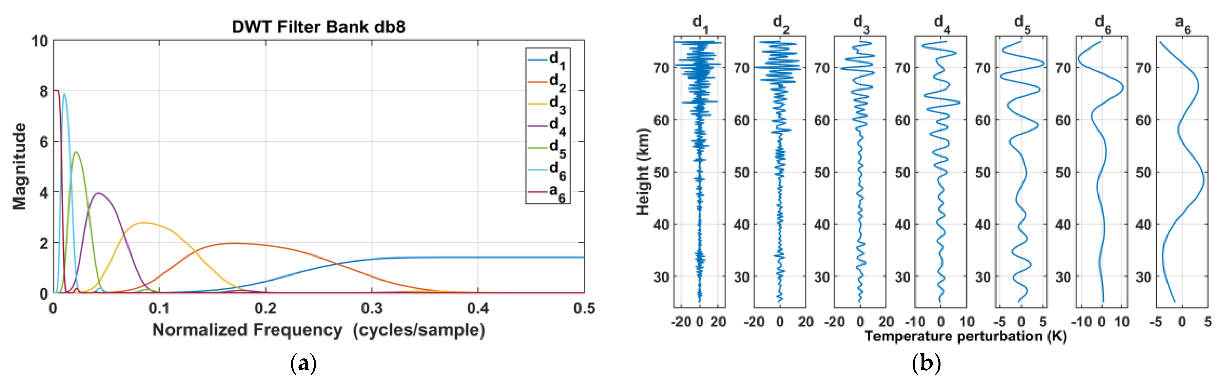
2.2. Analysis Methods: Processing and Methodology

The GW potential energy (GW-EP) is estimated from the variance of the fluctuations in the raw lidar signal, proportional to the GW-induced perturbations of atmospheric density and temperature. Details of the method are presented in Mze et al. [68]. Basically, the amplitude of the fluctuations is estimated from the difference between the lidar signal in a given atmospheric layer and the average signal of the two adjacent layers. The advantage of the variance method is that the contribution to the variance of the measurement noise can be accurately estimated from the statistical noise of the photon count. The lidar signal is binned vertically before computing the variance, defining a broad bandpass window [68].

Wavelet analyses such as the continuous wavelet transform (CWT) and the multiresolution analysis (MRA) are applied to observational and model data to analyze dominant vertical wavelengths of GWs with height. The CWT with the Morlet wavelet enables us to compute spectral lines of dominant GW modes. The methods are illustrated in [69,70]. In the present study, the MRA also called the discrete wavelet transform (DWT) uses the Daubechies wavelet of order 8 (db8) to decompose perturbation profiles into successive vertical wavelength bandwidths with details and an approximation. Figure 4 shows the vertical wavelength bandwidths expressed as normalized frequencies of the db8 orthogonal octave-band filter bank. The signal can be reconstructed perfectly as the sum of the details and the approximation. Figure 4b illustrates a sixth-order MRA with the db8 wavelet applied on a 15 min lidar temperature profile on the night 9 October 2017. With a vertical resolution of 150 m, the octave band iterated filters produce details with vertical wavelength bandwidths of 0.3–0.6 km (d₁), 0.6–1.2 km (d₂), 1.2–2.4 km (d₃), 2.4–4.8 km (d₄), 4.8–9.6 km (d₅), 9.6–19.2 km (d₆) and >19.2 km for the approximation (a₆). The two first details are more affected by noise in particular above 65 km height where GW breaking may occur. Several wavelike structures are highlighted in the other details such as a dominant mode of about 13 km vertical wavelength in the detail d₆ above 40 km heights. Thus, details iteratively extract multi-scale quasi-monochromatic GW structures from vertical profiles.

The WRF model version 3.9 with a triple two-way interactive nested grid of 27 km (domain D1), 9 km (domain D2) and 3 km (domain D3), centered on La Réunion, with a terrain elevation of 30 s resolution is used to simulate the specific meteorological event and related GWs with 6 min dynamical outputs from 8 October at 0600 UTC to 12 October at 1200 UTC (Figure 5). Settings for the WRF runs are summarized in

Table 1. Set-up for WRF options.

Option	Setting
Model code	version 3.9
Map projection	Lambert
Domain size and resolution	Domain D1—27 km, 160 × 119 grids Domain D2—9 km, 313 × 204 grids Domain D3—3 km, 793 × 468 grids
Vertical coordinates and vertical resolution	140 eta-pressure levels up to 10 hPa (32 km), resolution increasing from 20 m to 250 m up to 29-km height and 250 m above
Radiation	Long-wave Rapid Radiative Transfer Model (RRTM) Mlawer and short-wave Dudhia schemes
Microphysics	Single-Moment 6-class (WSM6) scheme
Cumulus	Kain-Fritsch scheme
Planetary Boundary Layer	Yonsei-University scheme
Surface layer	Noah Land-Surface Model scheme
Top layer condition	5-km Rayleigh damping
Lateral boundaries	6-hourly NCEP FNL analyses (31 isobaric levels up to 10 hPa, 1° × 1°grids)
Bottom layer condition	Fixed sea surface temperature

. The altitude range includes 140 eta-pressure levels up to 32 km height with a vertical resolution <250 m at heights <29 km. A 5 km Rayleigh damping layer prevents spurious reflections of GWs at the top of the model. The successive WRF outputs of the horizontal wind provide a detailed description of the subtropical jet split as well as its reconstruction from 11 October as it progressed eastward, South of Madagascar (Figure 5).

The meridional and zonal wavenumbers, the normalized frequency (the ratio between the frequency and the inertial frequency ω/f) and the amplitude of GWs are used as inputs to initialize rays in the GROGRAT model. The inertial period is about 33 h at the latitude of La Réunion. To identify GW tropospheric sources, the model is firstly initialized with background fields of the temperature, horizontal wind and geopotential altitude every 6 h from ERA5 model data with 37 pressure levels from 1000 to 1 hPa and horizontal resolutions of 0.25° × 0.25° for the region (43°E−67°E, 6°S−30°S). Secondly, ERA5 data with 137 levels are used to trace the vertical propagation of GWs from the stratosphere up to the top of the middle atmosphere.

The image processing software ImageJ (https://imagej.nih.gov/ij/, accessed on 7 april 2023) is used to retrieve manually observed GW parameters for small horizontal wavelengths from individual nightglow images, such as the axis of the horizontal propagation of detected waves, their horizontal wavelengths and the relative intensity along a profile from each corrected radiance night-glow image (Figure 6). The relative intensity is needed to compute the GW-EP. The observed phase velocity and direction of horizontal propagation are then obtained by analyzing several consecutive images. Parameters are corrected with the HWM14 model wind speed and direction at the OH layer altitude to obtain the intrinsic ones. Figure 6 shows evidence of a GW structure with a 4 km horizontal wavelength propagating along the yellow line. To study GWs with horizontal wavelengths exceeding the field of view of the image (170 km × 130 km), a keogram analysis is performed by considering the central columns (or central row) of each image and placing them side-by-side to form a single image [71].

This analysis provides the north–south (N/S) and east–west (E/W) keograms using the central column and row, respectively. The result presents the wave field during the night. Figure 7 visualizes wavelike structures of GWs on the N/S keogram during the night of 10 October 2017. Wave parameters are automatically processed when using spectral methods.

3. Results

3.1. MIL and GWs in the Middle Atmosphere on 9–10 October 2017

Lidar, nightglow and radiosounding datasets from June 2016 to April 2017 were scanned to select simultaneous high-quality and long duration observations in the presence and in the absence of a MIL above La Réunion. The night of 9 October 2017 reveals the presence of a MIL with an amplitude of about 30 K which disappears the next night. It was accompanied with a strong activity of GWs. Temperature lidar operated for nearly 5 and 4 h on 9 and 10 October, respectively. Figure 8a,b visualize the difference between the two consecutives nightly mean profiles. The MIL is characterized by a temperature minimum around 78 km and a warm layer above at heights of 80–87 km in comparison with the nightly mean profile of 10 October 2017. Figure 8c shows the five consecutive hourly profiles on 9 October. The MIL is present during the four first hours and starts to disappear during the last one from 1939 to 2041 UTC. Wavelike structures with large amplitudes on detail d₃ (Figure 4b) suggest possible signature of GW breaking from 65 km height on lidar profiles. The spatial extension of the MIL is investigated in analyzing the WACCM simulation. First, Figure 9a shows that temperature vertical profiles from lidar and WACCM on 9 October at 1800 UTC are in agreement. The model simulates some inversion layer starting at a height of about 79 km (black solid line). The map of the temperature gradient at an altitude of 79 km (Figure 9b) demonstrates that the inversion feature is spatially extended, with a local maximum of the gradient south of La Réunion, at least at 79 km altitude. At this location the simulated vertical temperature profile is also extracted and shown as a black dashed line in Figure 9a. The profile has a relative minima at around 80 km and 100 km altitude, respectively, and some inversion of the temperature occurs between both altitudes. Although such results from a unique case study above La Réunion should be taken with caution, the feature is likely to have a horizontal extent at least across many hundreds of kilometers.

Spectral lines are derived from 15 min Lidar temperature perturbation profiles on the two consecutive nights. Figure 10a,b identify a dominant mode with a vertical wavelength of about 10–15 km. Smaller wavelengths of about 3 km and 4–6 km are also observed during the observation night. Indeed, the DWT decomposition of the 15 min temperature perturbation profile at 1535 UTC clearly visualizes a quasi-monochromatic mode of about 12 km vertical wavelength on the detail d₆ above 40 km height (Figure 4b). Figure 10c visualizes height-time variation of long vertical wavelength disturbances > 5 km resulting from the subtraction between the smoothed night average and the integrated smoothed profiles over 30 min. A Hanning window of 51 points is also used to remove short vertical wavelength disturbances < 5 km. Then, details d₆ focus on the time–height variation of the dominant mode with a 12 km vertical wavelength (Figure 10d). A similar figure is obtained when details d₆ are filtered with a 4th order butterworth pass-band filter with a vertical wavelength bandwidth of 10–15 km. Figure 10d highlights a dominant GW mode with a vertical wavelength of 12–13 km, an observed period of about 5 h and a downward phase propagation (upward propagation of energy) on 9 October 2017 in the middle atmosphere at heights of 30–70 km. A two dimensional Fourier transform directly applied on the time–height distribution of lidar temperature perturbations also supports the presence of such a dominant mode (not shown).

The GW-EP provides a measure of GW activity during the two nights of lidar observation for vertical wavelengths of 2.5–8.5 km (Figure 11). Both profiles show a strong decrease in GW-EP between 47 and 50 km heights, indicating that dissipation mechanisms exist at the stratopause level. In both profiles an exponential increase in GW-EP is observed between 50 and 70 km heights almost following the expected increase without dissipation. The GW-EP is lower on 9 October in the upper stratosphere and the opposite is observed in the mesosphere. The highest GW-EP occurs in the mesosphere on 9 October when the MIL is present.

3.2. Sources of GWs and Vertical Propagation

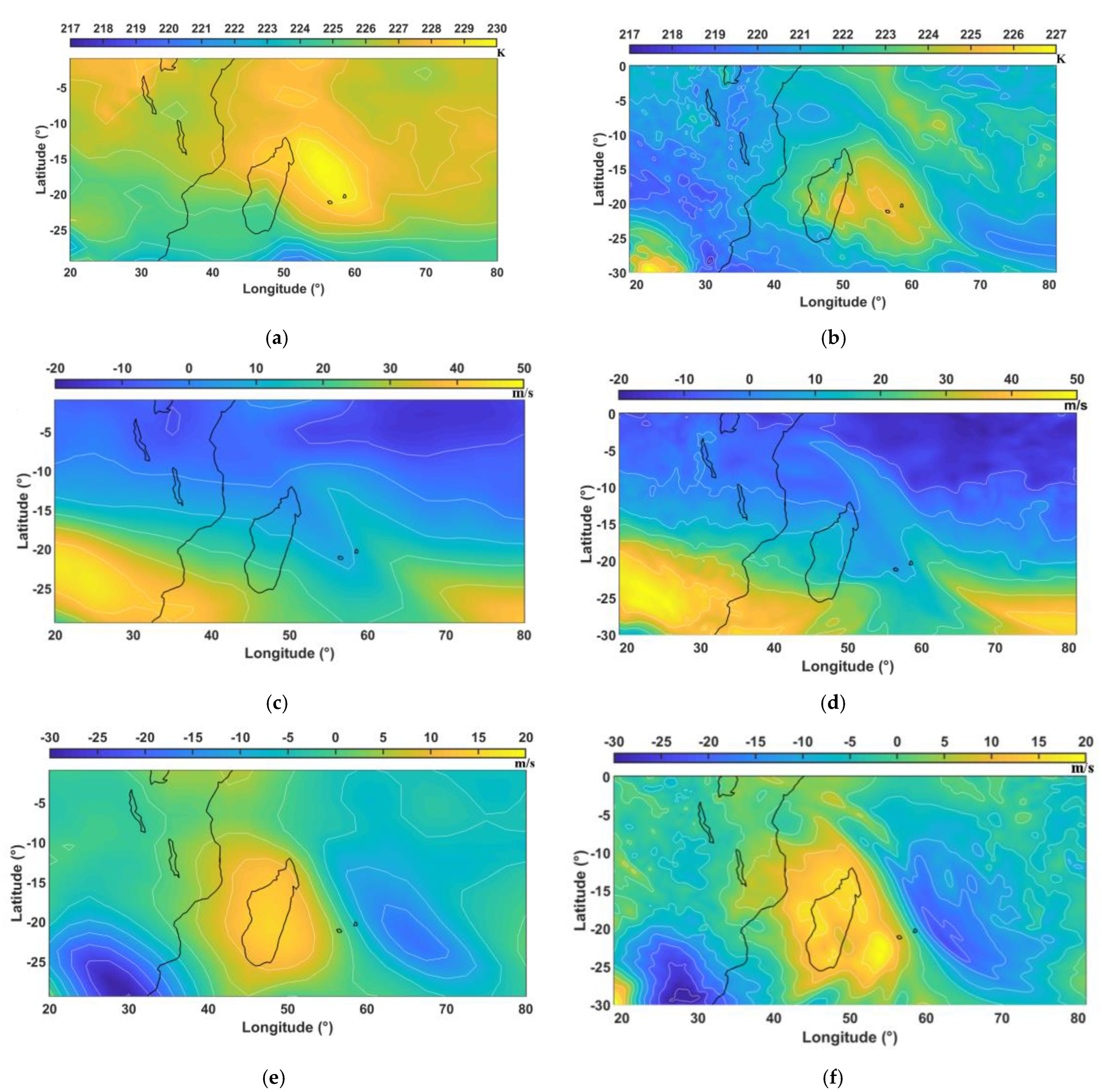
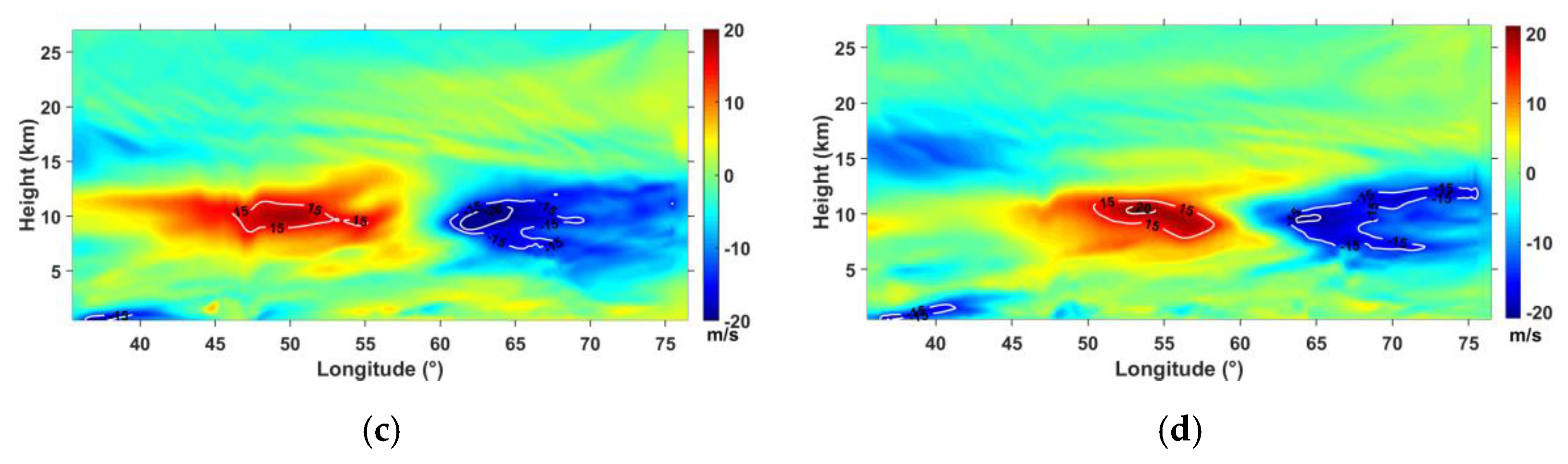
3.2.1. Synoptic Pattern and GW Parameters in the Troposphere and the Stratosphere

The austral winter 2017 (early May-late October) is globally characterized by the absence of humidity in the middle troposphere and the presence of the tropospheric subtropical westerly jet at La Réunion. The analysis of radiosonde wind perturbation profiles indicates that the GW kinetic energy density is large in the troposphere at heights of 5–15 km when the subtropical westerly jet becomes a dominant source of GWs in austral winter [70]. A strengthening of the activity of planetary waves affecting the polar vortex was reported during the austral winter 2017 [72,73].

The perturbed vortex led the subtropical jet to cross over South Africa from 9 to 11 October 2017. Rossby waves (white contours) with a horizontal wavelength of about 4500 km, a period of 5 days and a phase speed of −11 m/s were guided toward the tropics along the broken jet on 9 October (Figure 12a). In situ radiosonde data support that the subtropical jet above La Réunion is indeed perturbed on 9 and 10 October. Figure 12b visualizes two weakening periods of the zonal wind which correspond to ruptures of the subtropical jet in October 2017 due to the presence of Rossby waves at the subtropical barrier. Rossby waves break near the critical zonal wind intensity of ~10 m/s at heights of 10–15 km on 9 October above La Réunion (Figure 12a,c).

The event is characterized by the presence of a barometric trough around 65°E west of Mauritius which perturbed the Mascarene High and displaced it eastward from its climatological location. A tropical disturbance was strongly affected by the trough and the induced meridional wind shear in the middle troposphere until its evacuation poleward by the jet (Figure 12d). The synoptic pattern was reproduced by global numerical weather prediction models ERA5 and the climate model WACCM (Figure 2). Tropospheric RWB appears to be an important dynamical process for GW formation [74,75]. Local diabatic heating induced by RWB can generate or reinforce GW activity [76,77]. Climatological studies show that RWB occurs around the mean position of the dynamic tropopause (PV = −2 PVU) on the 350-K isentrope (13 km altitude above Reunion), below Madagascar and Reunion when the jet splits during September and October over the SWIO [78,79].

Horizontal wind perturbations are extracted from radiosonde data on 9 and 10 October (Figure 13a,b) and processed by the CWT (Figure 13c,d) to highlight dominant GW modes. Observation shows evidence of a dominant mode with maximum amplitudes of 7 m/s and a vertical wavelength of about 2–3 km at heights of 10–20 km. The axis ratio of the elliptical structure derived from the hodograph of horizontal wind on 10 October provides quasi-inertial periods of 19–25 h. Spectral lines also highlight other dominant modes in the lower atmosphere. In particular, modes with vertical wavelengths of 2–3 km, 4–7 km and 9–13 km are observed at heights of 18–28 km in the stratosphere. The dominant GW mode with a vertical wavelength of about 10–15 km, which has been observed in lidar data, is also detected in the troposphere. The hodograph of horizontal wind perturbations for the mode of ~4 km vertical wavelength visualizes an elliptical structure with an anticyclonic rotation with height on 10 October 2017 in the lower stratosphere (Figure 13e,f). This upward propagating GW has maximum amplitudes of wind perturbations at heights of 10–15 km in the middle troposphere. The axis ratio of 2.3 provides a period of about 14 h. The Fourier spectra of horizontal winds and temperature support the presence of observed GWs with vertical wavelengths <7 km at heights of 18–28 km on 10 October 2017 with a dominant south-eastward horizontal propagation (Figure 14). The vertical-wavenumber spectra of normalized temperature fluctuations on 9 and 10 October agree well with the saturation limit [80] which may favor energy transfer to the background atmosphere. The mean m-slope is about 2.2 and about 3 for the periods of 4–9 October and 9–15 October, respectively. Mean spectral characteristics of GWs in the upper troposphere and the stratosphere are derived from radiosonde vertical profiles using the analysis methods described in [81,82]. The temperature and wind fluctuations are extracted from the raw profiles using a polynomial of order 1 and 2, respectively, to produce mean vertical profiles. Modes with vertical wavelengths of 1.7 km, 2.6 km and 4–5 km with periods of 5–27 h are computed at heights of 18–28 km with a dominant south-eastward horizontal propagation. The upward propagating energy flux is estimated at about 80% and 68% on 9–10 October at heights of 20–25 km and 20–28 km, respectively. Thus GWs are mostly produced at heights < 20 km and propagate upward in the stratosphere. The total energy density values of 2.5 Jkg⁻¹ and 5.3 Jkg⁻¹ at heights of 20–25 km and 20–28 km, respectively, are quite consistent with those derived from lidar observation at the lowest altitudes. The analysis of mean parameters focuses on short vertical wavelengths < 10 km and low frequencies especially because of the altitude range of 10 km in the lower stratosphere and the detection of GWs based on elliptical structures, respectively. The dispersion relation provides horizontal wavelengths in the range between 200 km and 1300 km.

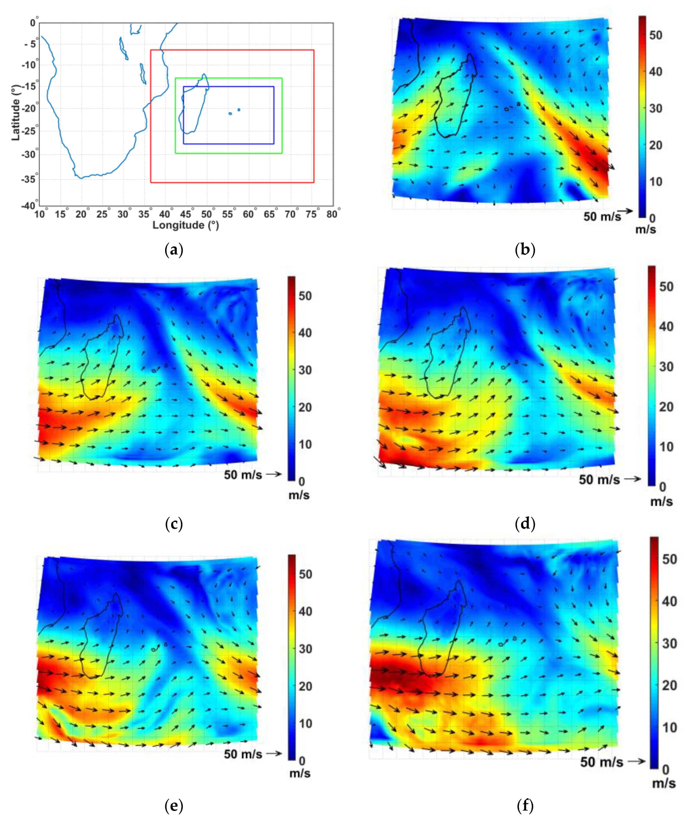
3.2.2. Mesoscale Modeling in the Troposphere and the Stratosphere

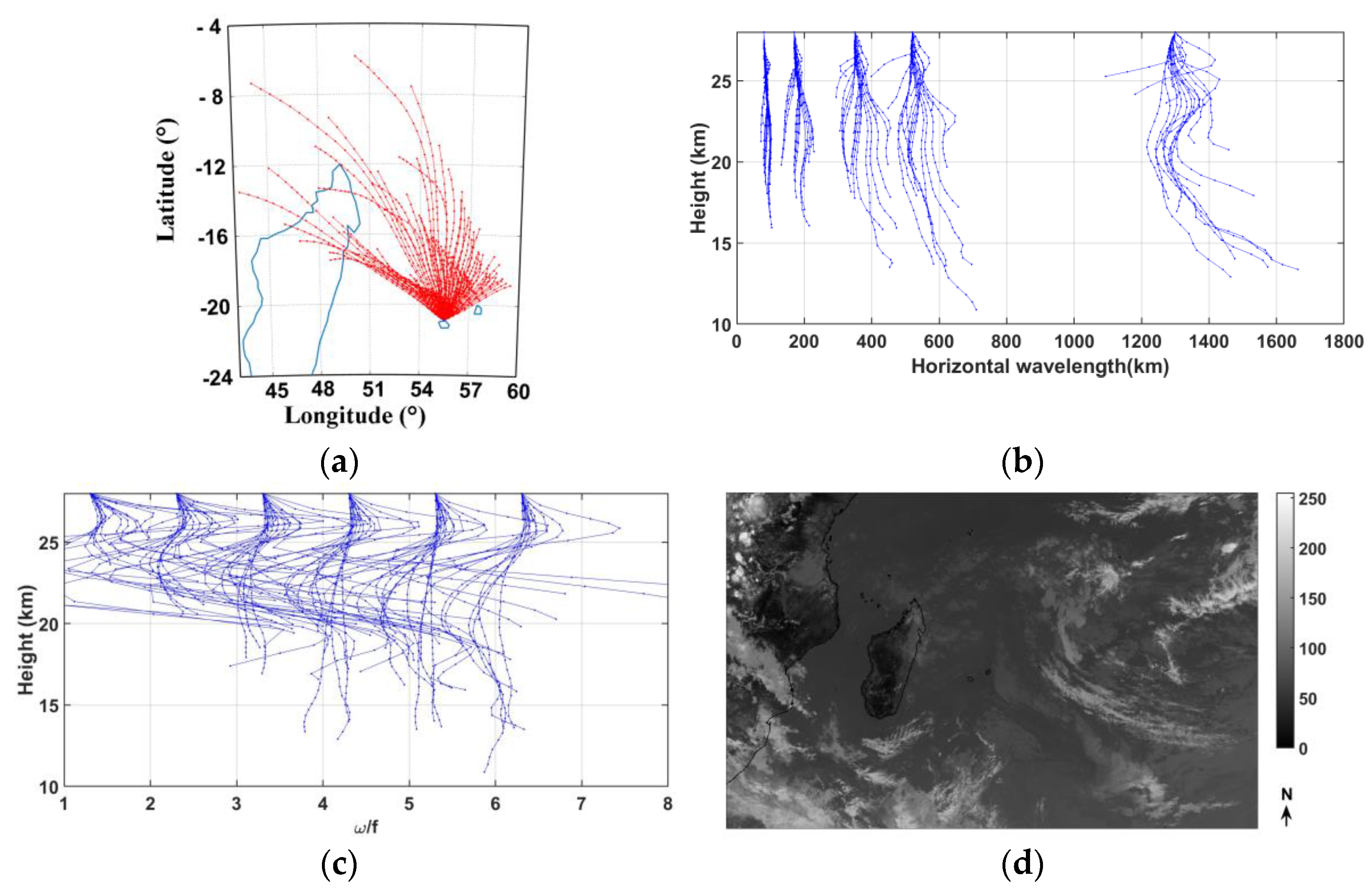
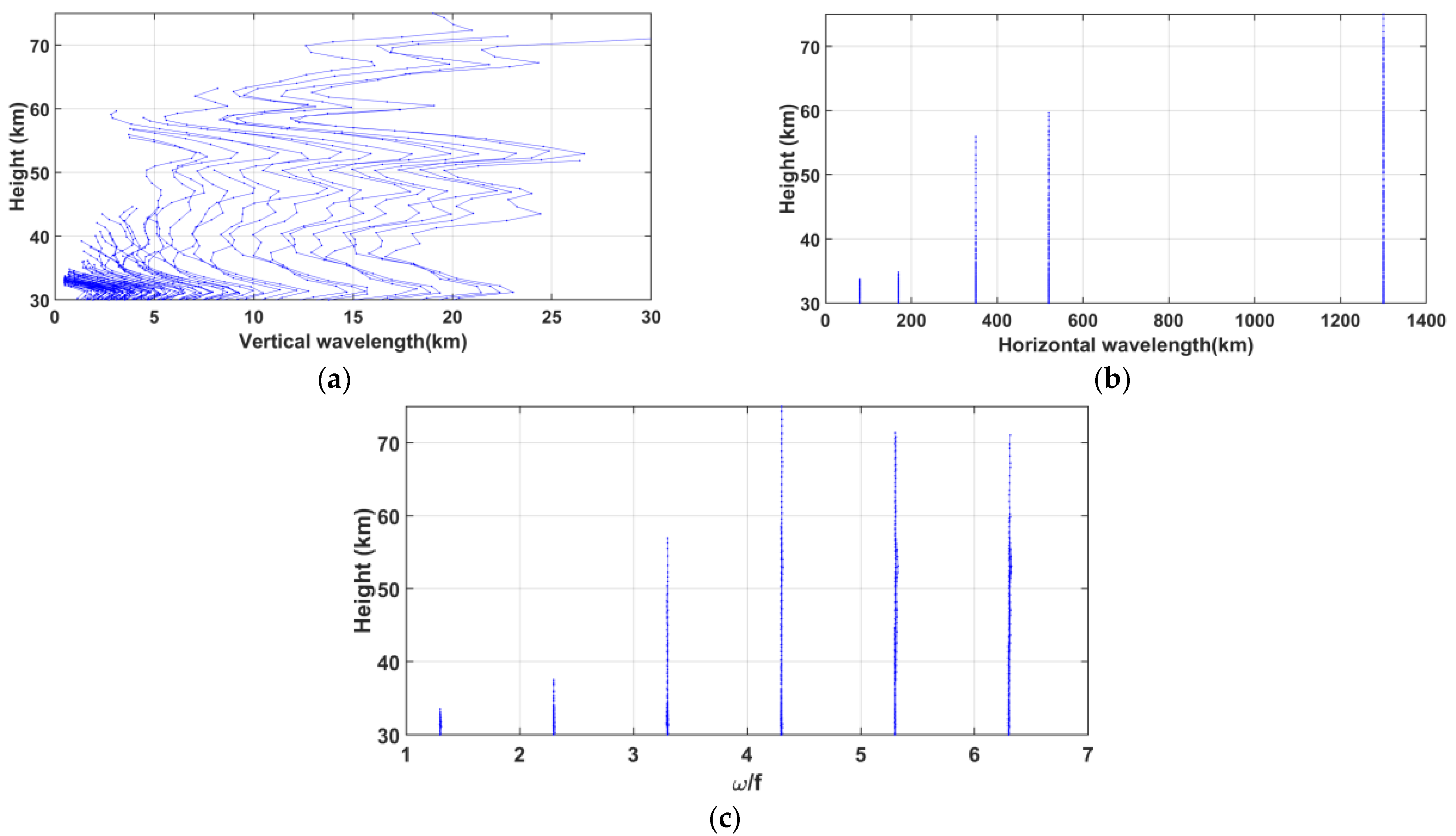
Simulated atmospheric background horizontal wind is shown to be in agreement with hourly ERA5 data during the simulation period (Figure 15). Comparison between WRF and ERA5 outputs indicates that the weakening of the zonal wind and the strengthening of the meridional wind at 10 km height are well reproduced in time and intensity from 9 October at 1200 UTC to 11 October at 1200 UTC above La Réunion. The mesospheric zonal wind also weakens while the stratospheric zonal wind strengthens from 9 October in the ERA5 dataset. The evolution of the stratospheric zonal wind is consistent with observations of radiosonde (Figure 12b) and WRF (Figure 15a) at the top level. In addition, the comparison between vertical profiles of WRF and observed horizontal winds on 9 and 10 October at 1130 UTC indicates that mean profiles of zonal and meridional wind are consistent in the troposphere and the lower stratosphere at heights between 3 km and 30 km above La Réunion.

In particular the model simulates the meridional wind shear which is observed on the radiosonde vertical profiles on 9 and 10 October at an altitude of 10 km (Figure 1b,c). The widths of the peak are quite similar and the amplitudes are 15 m/s and 20 m/s on 9 and 10 October, respectively, in comparison with observed values of 25 m/s and 20 m/s. Figure 16a,b zoom on the Rossby wave pattern and the horizontal wind which were previously described from WACCM and ERA5 data (Figure 2e,f) on 9 October and 10 October above La Réunion. Successive 6 min outputs reveal that the formation of the subtropical jet centered at the latitude of 27°S west of Madagascar is slowed down on 9–10 October when Rossby waves are steady and break with local heating at heights of 10–12 km above La Réunion (Figure 16a,b). Rossby waves above La Réunion are completely dissipated on 12 October when the subtropical jet is south of La Réunion and continues its progression eastward. As the local northward jet moves eastward and is getting closer to the local southward jet on 9–10 October above La Réunion, wind intensities of the local jets as well as the wind shear in the meridional wind intensify (Figure 16c,d). During this period, short-scale wavelike structures are clearly observed in the lower stratosphere above the boundary between the two local jets (Figure 16c).

The MRA is applied on successive vertical profiles depicted in Figure 16c to focus on structures with vertical wavelengths of 0.8–3.2 km (d₃ + d₄) on the background wind (d₇ + a₇). Thus, Figure 17a highlights the presence of GWs with a vertical wavelength of about 2.5 km, which are embedded in the inner cores of the tropospheric local jets. Indeed, the simulation produces short-scale wavelike structures in the meridional wind with dominant vertical wavelengths of 4–7 km on 9 and 10 October at 1200 UTC at heights in the troposphere and the lower stratosphere (Figure 17b). Another dominant mode with long vertical wavelengths of about 10–13 km is also simulated during this period. The hodograph of stratospheric horizontal wind perturbations on 9 October at 1200 UTC above La Réunion supports the presence of short-scale GWs (Figure 17c) with a vertical wavelength of ~2.5 km and an upward energy propagation in the lower stratosphere. Figure 17d pictures the MRA details with vertical wavelengths of 0.8–3.2 km only. It shows that the meteorological event produces tropospheric GWs with a dominant vertical wavelength of ~2.5 km, which propagate upward in the stratosphere. The downward phase progression to the east suggests that GWs mostly propagate eastward. For vertical wavelength bandwidths of 3.2–6.8 km and 6.4–12.8 km, large amplitudes of GWs with vertical wavelengths of 4–5 km (Figure 17e) and 10–11 km are observed at heights of 10–12 km (not shown). Moreover, ERA5 data also support the production of GWs in the troposphere with a vertical wavelength of about 11–12 km above La Réunion (Figure 17f). The figure shows evidence of a downward phase progression to the east and upward propagation in the mesosphere up to 70 km height. The amplitude of the structure increases at heights of 40–50 km, probably due to the partial reflection of GWs near the stratopause. Periods of GWs are computed near the main source at the height of 11 km from the time series of zonal and meridional wind perturbations from 9 October at 0000 UTC to 10 October at 0300 UTC and from 10 October at 0000 UTC to 11 October at 0300 UTC (Figure 18a). The kinetic energy density of GWs is mainly produced by the meridional wind. Dominant periods vary between 5 h and 20 h on 9 and 10 October. Similar periods are also observed in the lower stratosphere at heights of 25–28 km with a dominant period of 6 h (Figure 18b). Moreover, Figure 18b shows evidence of a dominant 10 h period in the middle troposphere, especially at heights of 9–11 km. At this range of altitudes, the trend of mean kinetic energy from 9 October to 12 October supports that the intense period of GW activity occurs from 9 October to 11 October in the meridional wind (Figure 18c). In addition, Figure 18c reveals oscillations with periods of 5–10 h superimposed on the trend. A large amplitude of this oscillation is observed in the meridional wind during the intense period of GW activity as well as during the nights of lidar observation. At heights of 14–24 km above the GW source, Figure 18d visualizes banded patterns with a wavelength of ~3 km in the kinetic energy of the meridional wind on 10–11 October, which are indicative of a GW structure with a vertical wavelength of ~6 km. Such structures are also produced above the tropospheric GW source with upward propagation into the stratosphere on 9 October.

3.2.3. Raytracing

The raytracing technique is now performed to investigate main GW sources and upward propagation into the middle atmosphere from GW characteristics in the lower stratosphere using GROGRAT. About 90 modes are released at the altitude of 28 km above La Réunion on 9 October at 1200 UTC to describe GW propagation in the lower atmosphere. The initialization of GW spectral characteristics are based on those derived from radiosonde and WRF data namely horizontal wavelengths of 80, 170, 350, 520 and 1300 km, normalized frequencies ω/f between 1.3 and 6.6 (with a step of 1, corresponding to the period range of 5–22 h) and south–east horizontal propagation direction of 120°, 150° and 170° (clockwise from North). Rays are integrated backward and forward in time to investigate tropospheric sources and the upward propagation of GWs into the middle atmosphere, respectively. The comparison between temperature and horizontal wind profiles derived from radiosounding and ERA5 above La Réunion on 9 October at 1118 UTC and 1100 UTC, respectively, indicates that ERA5 provides a good representation of the atmospheric background below 30 km heights.

The back-trajectories reveal that these modes originated from the upper and middle troposphere northward. They are mostly confined above the local heating in the temperature on 9 October (Figure 19a) where planetary waves break and the convective activity is low (Figure 19d). Some of them may be attributed to local convection above the northern region of Madagascar. The modes with frequency ratio ω/f > 4 (T < 7 h) and horizontal wavelengths >400 km, can take less than 12 h on 9 October to propagate from the middle troposphere to the altitude where rays are released in the stratosphere (Figure 19b). The simulation, with solely vertical propagation, time-independent back-ground and a horizontal wave direction constant with height, is run including a saturation scheme and turbulent and radiative wave damping for heights of 20–70 km [45,50]. Vertical wave propagation suggests that modes with periods of 5–10 h (3.5 < ω/f < 7), horizontal wavelengths > 350 km and vertical wavelengths >5 km can reach the mesosphere during the night of observation (Figure 20). Dominant vertical wavelengths vary between 7 and 15 km and 15 and 25 km at heights of 60–65 km and 70 km, respectively.

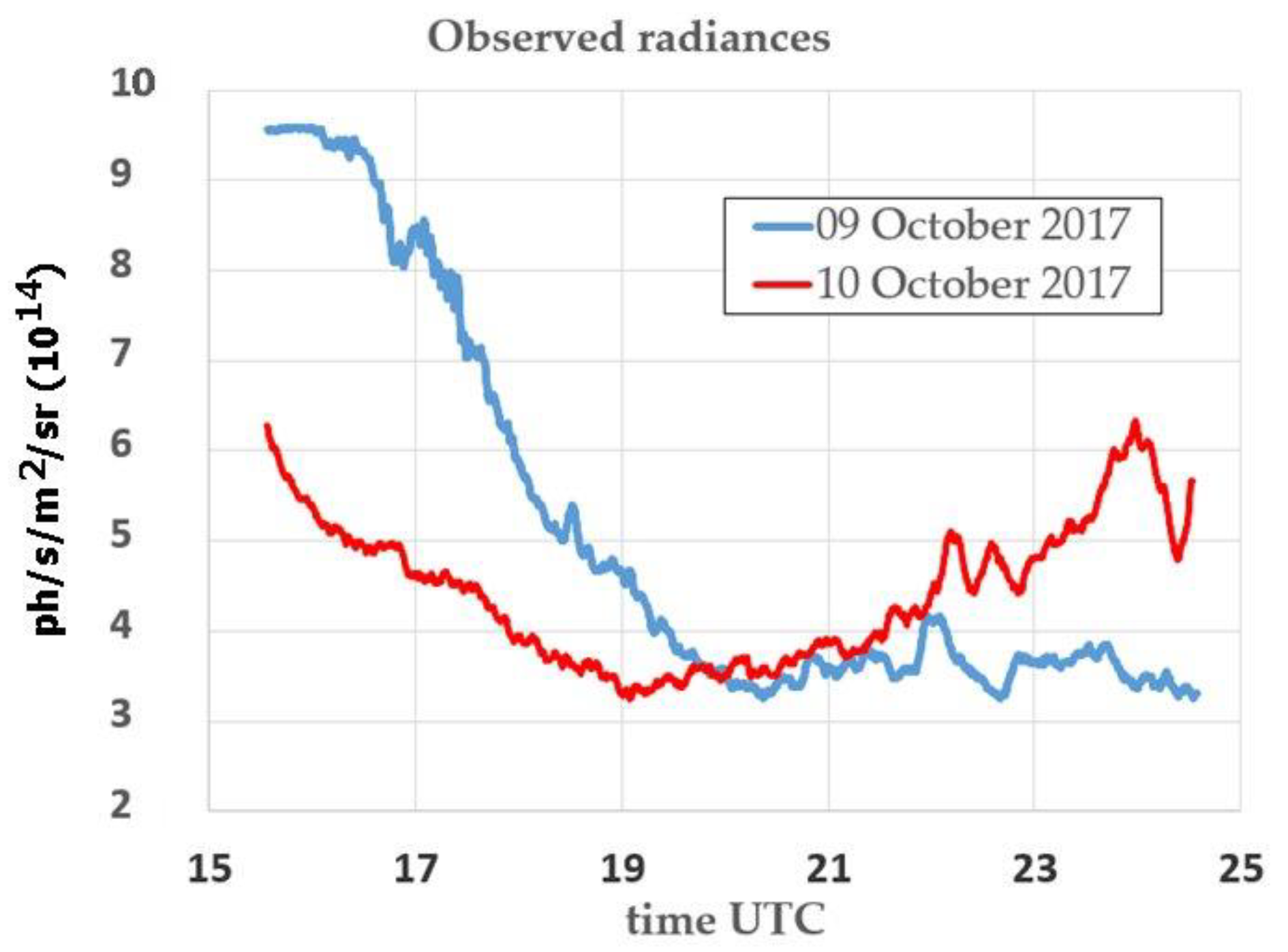
3.3. GW Activity in the Airglow Measurements

The OH 1.6 μm and 2.0 μm volume emission rate (mainly corresponding to Δν = 2 transition) and associated temperature vertical profiles are extracted from the SABER data from 9 October 2017 at 1455 UTC to 11 October 2017 at 2223 UTC (Figure 21a). Figure 21b shows evidence that SABER temperature and OH VER profiles are strongly affected by the GW activity during the studied period. Moreover, the profiles (orbit 85851) on 9 October 2017 at 1459 UTC highlight a dominant GW with a vertical wavelength of 4–5 km in the mesosphere up to 100 km in the lower thermosphere on the temperature and OH VER vertical profiles. The MRA is applied to the vertical profile of temperature to extract other possible wavelike signatures in the upper mesosphere at heights of 57–73 km and in the mesopause at heights of 77–96 km where the OH layer is located (Figure 21c,d). In the upper mesosphere, dominant modes with vertical wavelengths of 5.5 km and 12 km are observed in the details of d₃ and d₅ up to 73 km in height (Figure 21c). In the mesopause—lower thermosphere, dominant modes with vertical wavelengths of 4.5 and 10 km are observed in the details d₃ and d₄ (Figure 21d). Indeed, Fourier spectra derived from the perturbation profile (2nd panel from left) support the MRA. In addition, shorter and broader range wavelengths are observed in the mesopause in comparison with the upper mesosphere, probably because of secondary GWs generated by wave breaking.

At the OH layer at the height of about 87 km height, nightglow images show a decrease in the mean radiance up to midnight local time (1910 UTC) on the nights of 9 and 10 October which could be attributed to the OH photochemical decrease and to dynamical effects (Figure 22). The mean radiance is computed at the center of each nightglow image representing a surface area of 5.3 km x 5.3 km at the OH layer altitude. Small variations of the radiance are induced by GWs. For the 10 October (in red), the increase in the radiance can be attributed to an increase in the GW activity, as already observed during an experiment campaign held in India in May 2014 [83]. This behavior is directly observable on the keogram of Figure 7 close to 2200 UTC where structures are clearly visible. This implies a high variation of the relative intensity during this period and consequently a strong activity of GWs.

In fact, large amplitudes in the details d₁ suggest possible GW breaking in the upper mesosphere and the mesopause at heights of 62–68 km below the MIL and 84–90 km, respectively.

Table 2. GW parameters for 9 October 2017. First columns provide serial number, time of observation, horizontal wavelength (λ_h), observed phase speed (Vφ_obs), observed direction of propagation (θ_obs), observed period (τ_obs) and the relative intensity (dI/I). Intrinsic parameters (phase speed, direction of propagation, period) and vertical wavelength are gathered in the columns 8 to 11.

Serial	Time (UTC)	λh (km)	Vφobs (m/s)	θobs (°)	τobs (min)	δI/I	Vφi (m/s)	θi (°)	τi (min)	λv (km)
1	1613–1630	8	24	70	5.5	0.089	10.7	45	12	24
2	1630–1705	10	33	82	5	0.085	18	77	9	m2 < 0
3	1632–1735	10	47	115	3.5	0.088	40	118	4	m2 < 0
4	1747–1830	8	38	120	3.5	0.069	39	117	3.3	m2 < 0
5	1845–2040	16	37	57	7	0.053	46	61	5.7	17

gathered the observed and intrinsic GW parameters deduced from a series of nightglow images using ImageJ software. Intrinsic parameters are obtained after correction with the following Doppler relation between intrinsic frequency ω and observed frequency ω_obs:

ω = ω_obs − ku − lv

(1)

where k and l are, respectively, the zonal and meridional wavenumbers, and u and v are, respectively, the mean zonal and meridional local wind speeds at the OH layer altitude.

The wind speed is estimated with the empirical model HWM14. Table 2 provides typical values of horizontal wavelengths and observed phase speed ranging from 8 to 16 km and 27 to 47 m/s, respectively. This result, which is in contradiction with the propagation of GW theory, could be induced by a bad evaluation of the wind at the OH layer altitude. Moreover, the square of the vertical wavenumber is negative for nightglow series 2, 3 and 4 which could be a consequence of the bad evaluation of the wind and/or due to the filtering of the GWs by the mesospheric inversion layer. The vertical wavenumber is estimated from the GW dispersion relation. During one hour from 2050 UTC, ripples perpendicular to the wave system are visualized.

The spectral analysis of the N/S and E/W keograms was performed using two different methods. In the first method, the power spectral density (PSD) for each line is calculated and then summed and averaged by the number of lines (Figure 23a) [84]. This analysis shows significant peaks at 3.7 and around 6 min, as well as 19, 28, 42, 60 and 126 min.

A second method based on a 2D periodogram analysis of the keograms [85] reveals small values of temporal frequencies of 0.0020, 0.0073, 0.014, 0.023, 0.027, 0.033, 0.038 and 0.043 min⁻¹ which correspond to periods of 477, 136, 68, 48, 36, 30, 26 and 23 min, respectively (Figure 23b). Short periods are in agreement with the first analysis. In addition, long periods up to 8 h can be detected using this method; however this value should be used with caution as it corresponds to the total duration of the acquisition. To analyze GW activity along the night of 9 October, Figure 23c visualizes the N/S keograms before and after 1910 UTC. The PSD is larger before midnight which suggests a variation of GW activity during the night. Thus, stronger GW activity occurs in the first period of the night with smaller periods. Results obtained using ImageJ software are gathered in

Table 3. Same as Table 2 but for 10 October 2017.

Serial	Time (UTC)	λh (km)	Vφobs (m/s)	θobs (°)	τobs (min)	δI/I	Vφi (m/s)	θi (°)	τi (min)	λv (km)
1	1619–1643	15		130		0.04	14	263	17	0.3
2	1645–1734	17	4	120	70	0.09	3.3	69	84	1.2
3	1744–1820	8	19	-130	7	0.06	16	227	8	9
4	1857–1930	10	16	-108	10	0.08	6	221	27	5.8
5	2007–2036	11	30	135	6	0.07	45	118	4	19
6	2100–2206	13	7	125	30	0.12	30	101	7	2.2
7	2150–2350	14	6	-52	38	0.15	23	93	9	1.9

for the night of 10 October. At the beginning of the night, a quasi stationary GW moving toward the northwest is observed but after wind correction, the wave moves westward with an intrinsic phase speed of about 14 m/s. Nevertheless, the calculated vertical wavelength is very small (0.3 km), which forbid the evaluation of the potential energy Ep (Equation (2)) using the cancelation factor CF:

$${\mathrm{E}}_{\mathrm{p}}=\frac{1}{2\mathrm{C}{\mathrm{F}}^2}{(\frac{\mathrm{g}}{\mathrm{N}})}^2{(\frac{\mathrm{d}\mathrm{I}}{\mathrm{I}})}^2$$

(2)

where CF is the cancelation factor [86] depending on the vertical wavelength λv.

The validity of Equation (2) is for λv > 10 km, so along the night, the potential energy could be calculated for serial 5 only with λv = 19 km (CF = 0.49), leading to a value of Ep = 2200 J/kg. Extrapolation of the GW-EP without dissipation plotted in Figure 11 gives a value of 1600 J/kg for the altitude of 87 km, which is quite consistent with that calculated from the nightglow measurements. The PSD of the two keograms N/S and E/W (Figure 24) also exhibits some different tendencies, as shown in Figure 23a. The general tendency of the PSD follows the −5/3 evolution for periods greater than 2 min. We observe a clear increase in the PSD for periods greater than 5 min, probably induced by dynamic processes. Clearly visible peaks are detected for periods 6, 12, 42, 56 and 72 min. Same as the previous night, these periods are confirmed by the periodogram method. Unlike the night of 9 October, the PSD is larger after 1900 UTC than before and for observed periods greater than 8 min (Figure 24b).

4. Summary and Conclusions

The present work focused on a case study of a MIL and GW dynamics coupling the lower atmosphere to the mesopause in the lower thermosphere. The GW activity was induced by a RWB at the subtropical barrier on 9 and 10 October 2017 during austral winter over the SWIO. The need to combine multi-instrumental observations and modeling to describe the dynamical coupling from the lower atmosphere up to the lower thermosphere is evidenced.

The main results of the MIL and the related GWs on 9–10 October 2017 are listed below:

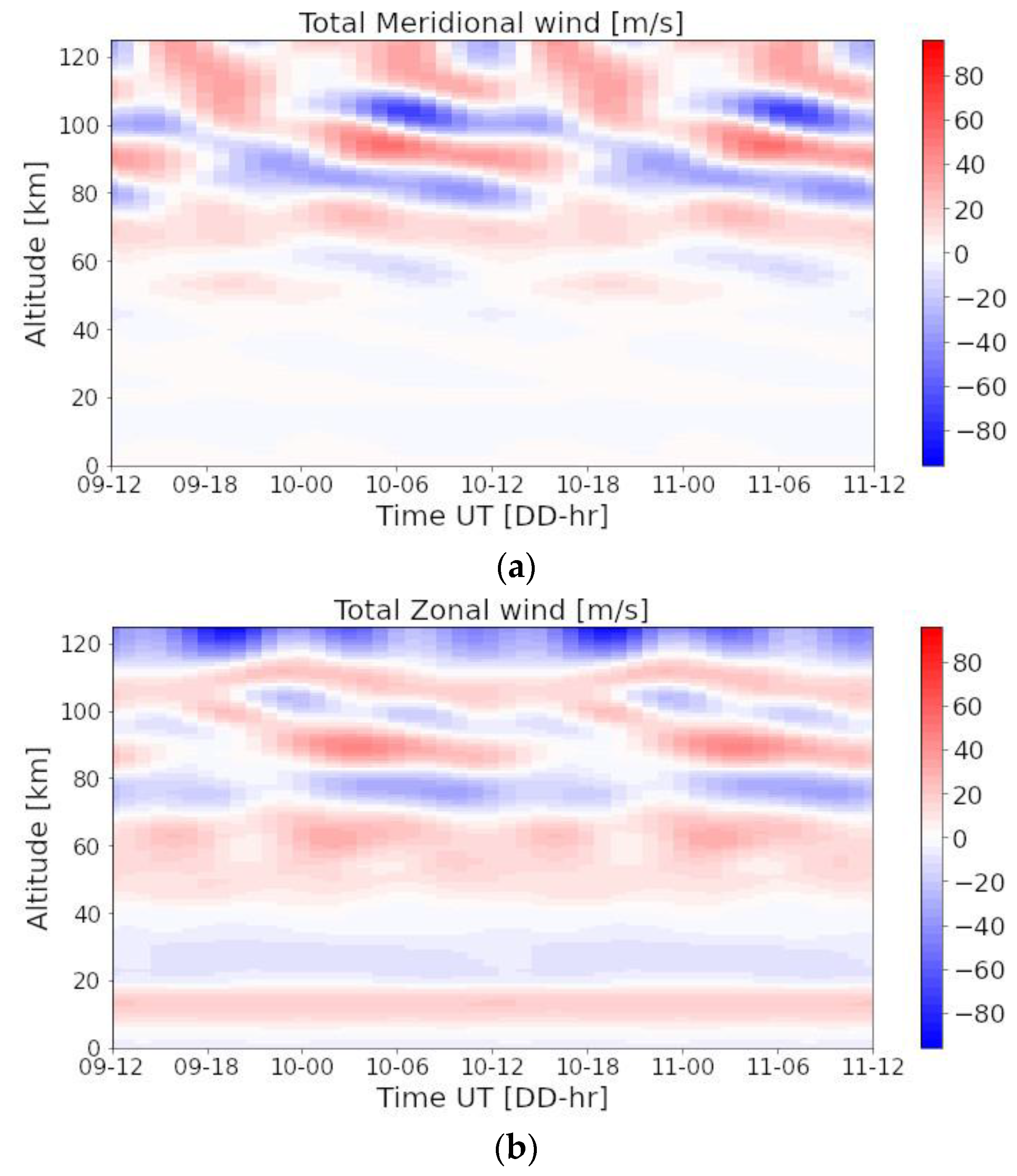
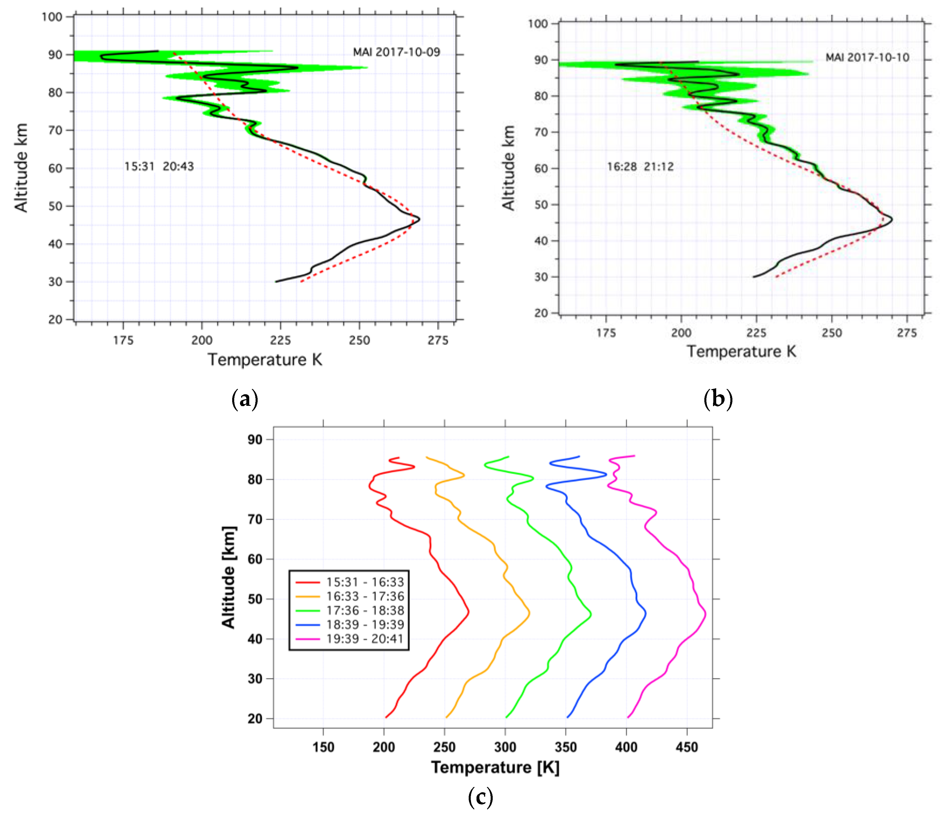
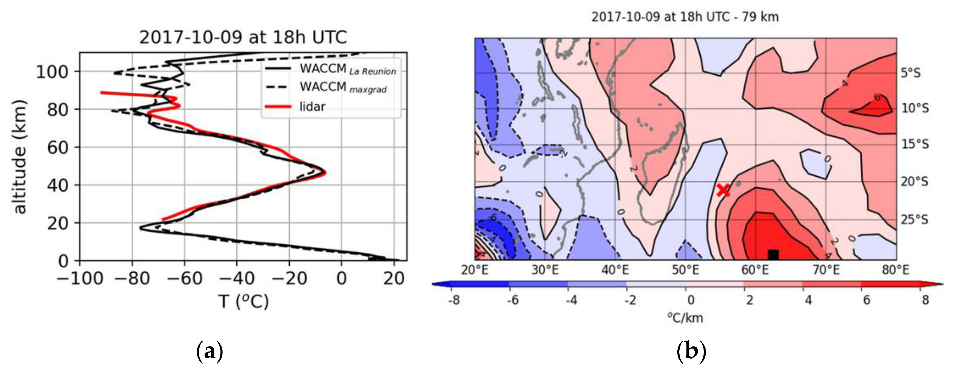
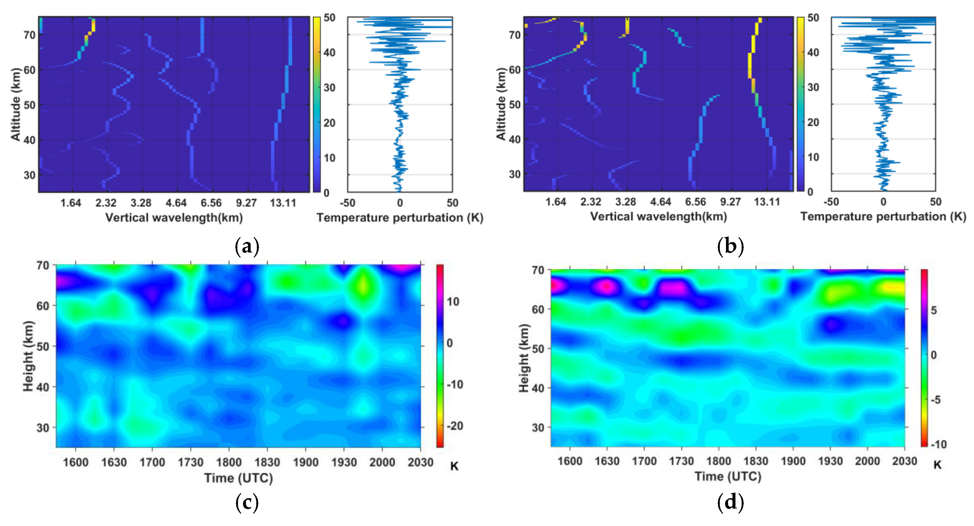
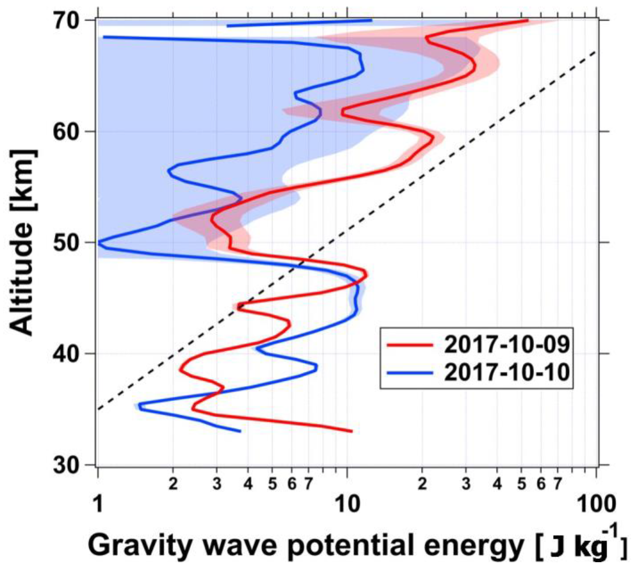
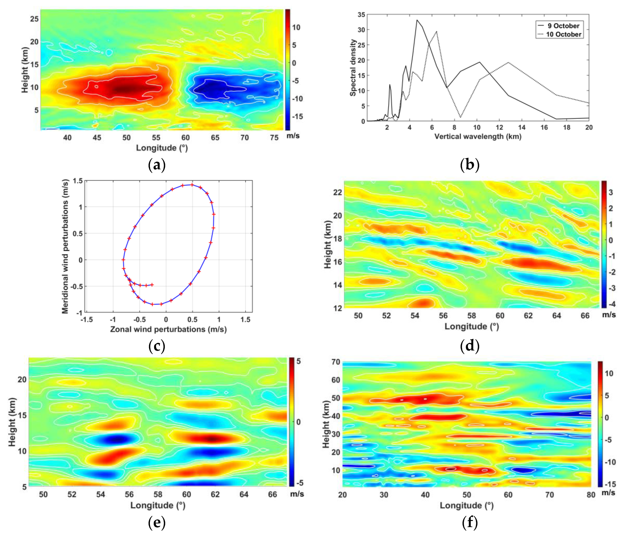
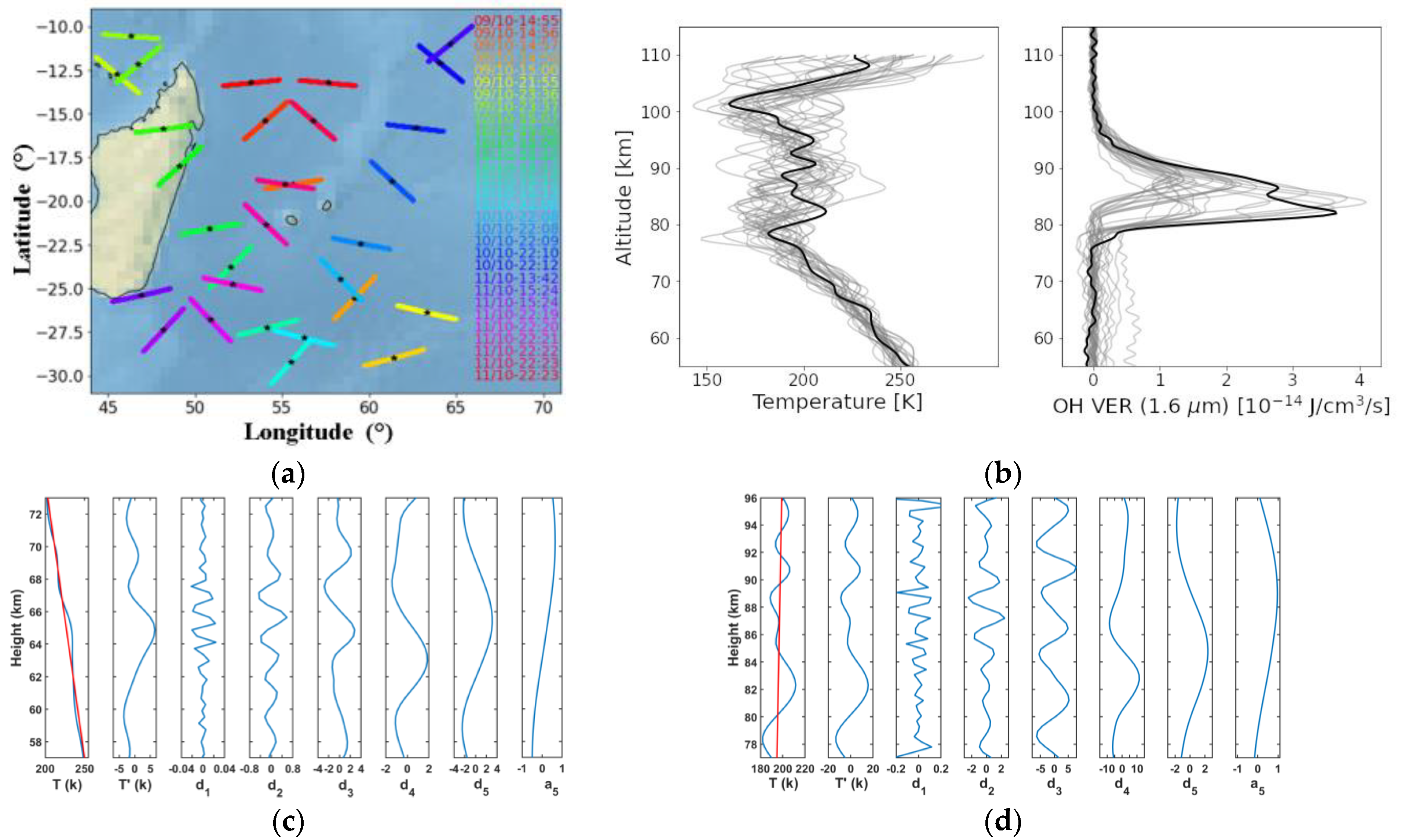
• In the middle atmosphere, Rayleigh lidar observation revealed the presence of a MIL with an amplitude of about 30 K at about 80 km height in the upper mesosphere on 9 October 2017 which disappeared on the next day. Dominant modes with vertical wavelengths of about 3 km, 4–7 km and 12–13 km were observed on lidar temperature profiles. Successive Lidar temperature profiles showed evidence of dominant GW mode with a vertical wavelength of 12–13 km on 9 October 2017 with a downward phase progression and an observed period of ~ 5 h at heights of 30–70 km in the upper stratosphere and the mesosphere. Dissipation mechanisms or wave reflection were reported at the stratopause level. Modeling with WACCM showed a spatially extended inversion feature at the altitude of the MIL above La Réunion. Signatures of GW breaking from 65 km height supported GWs as the main wave dynamical process of the MIL. Additionally, weather and mesoscale modeling suggested that the stratospheric filtering by the background wind was the possible cause for the disappearance of the MIL on 10 October 2017.
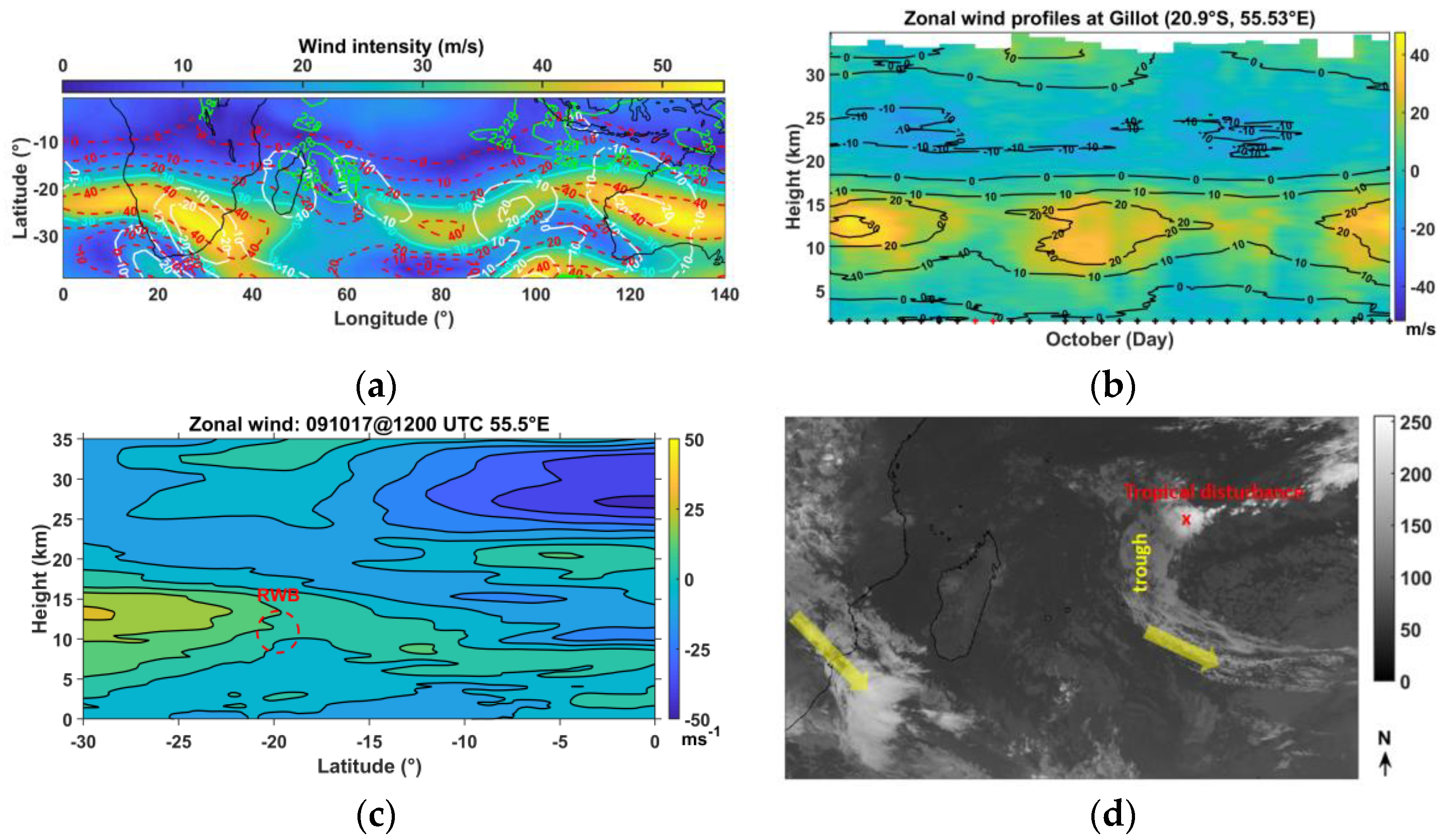
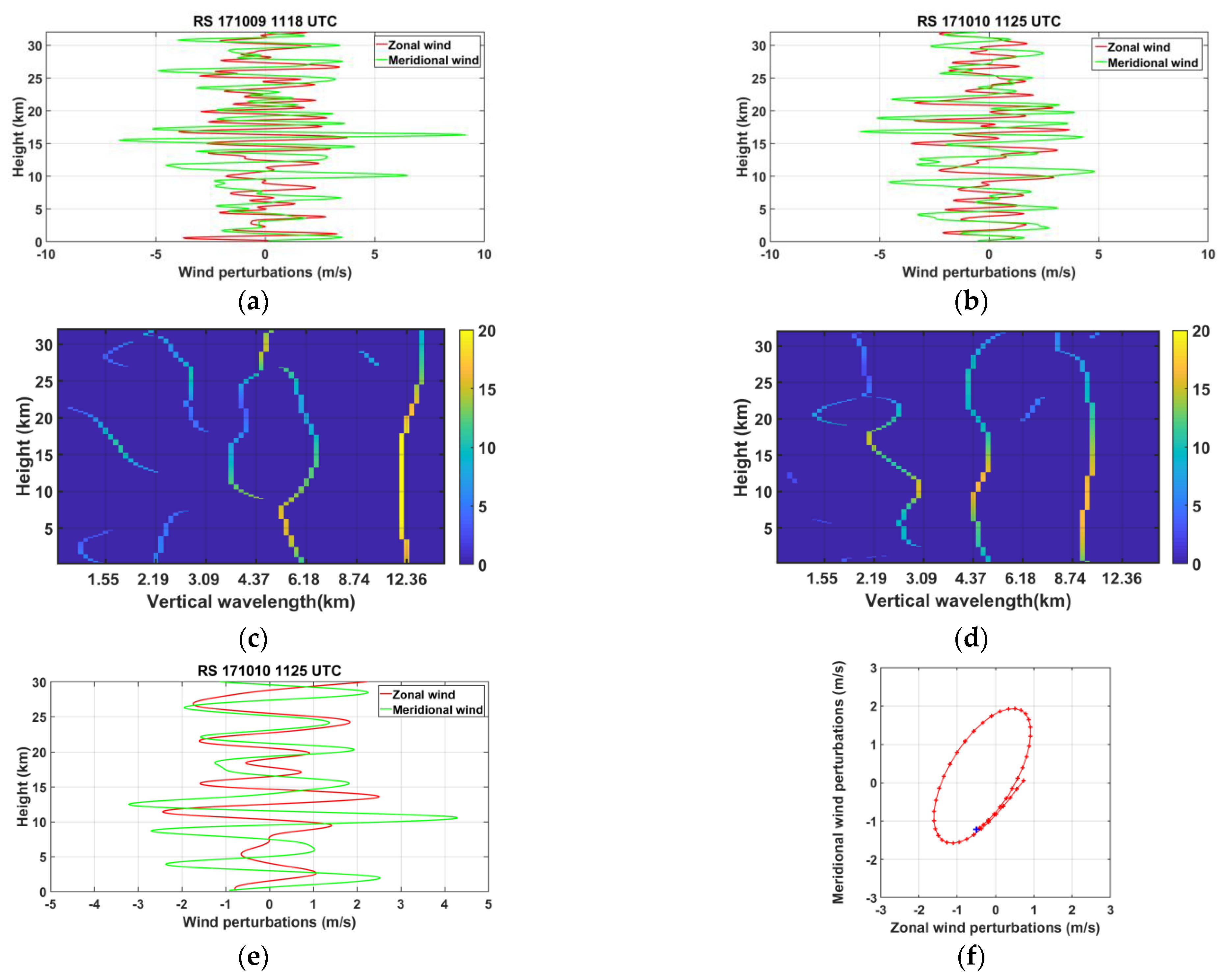
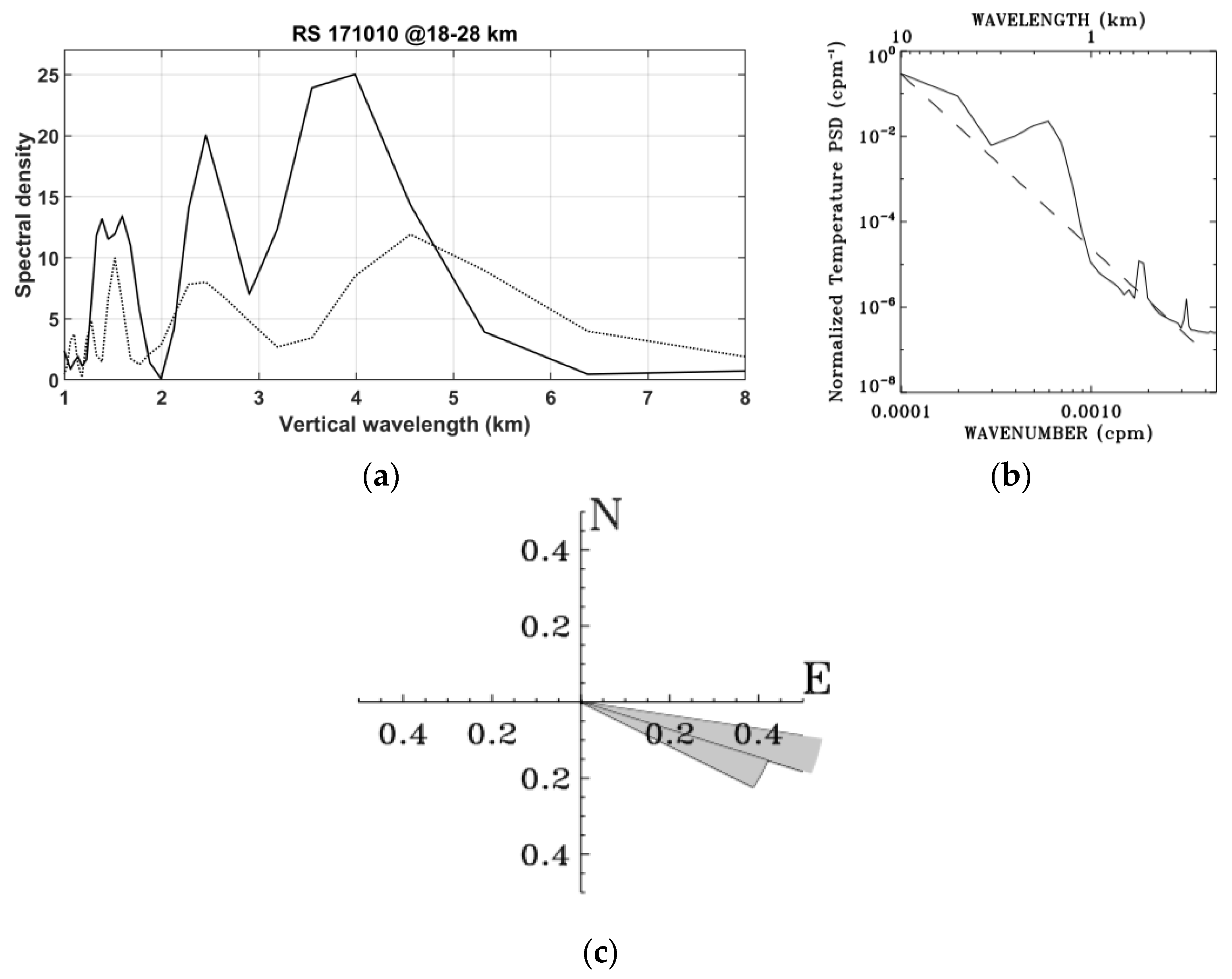
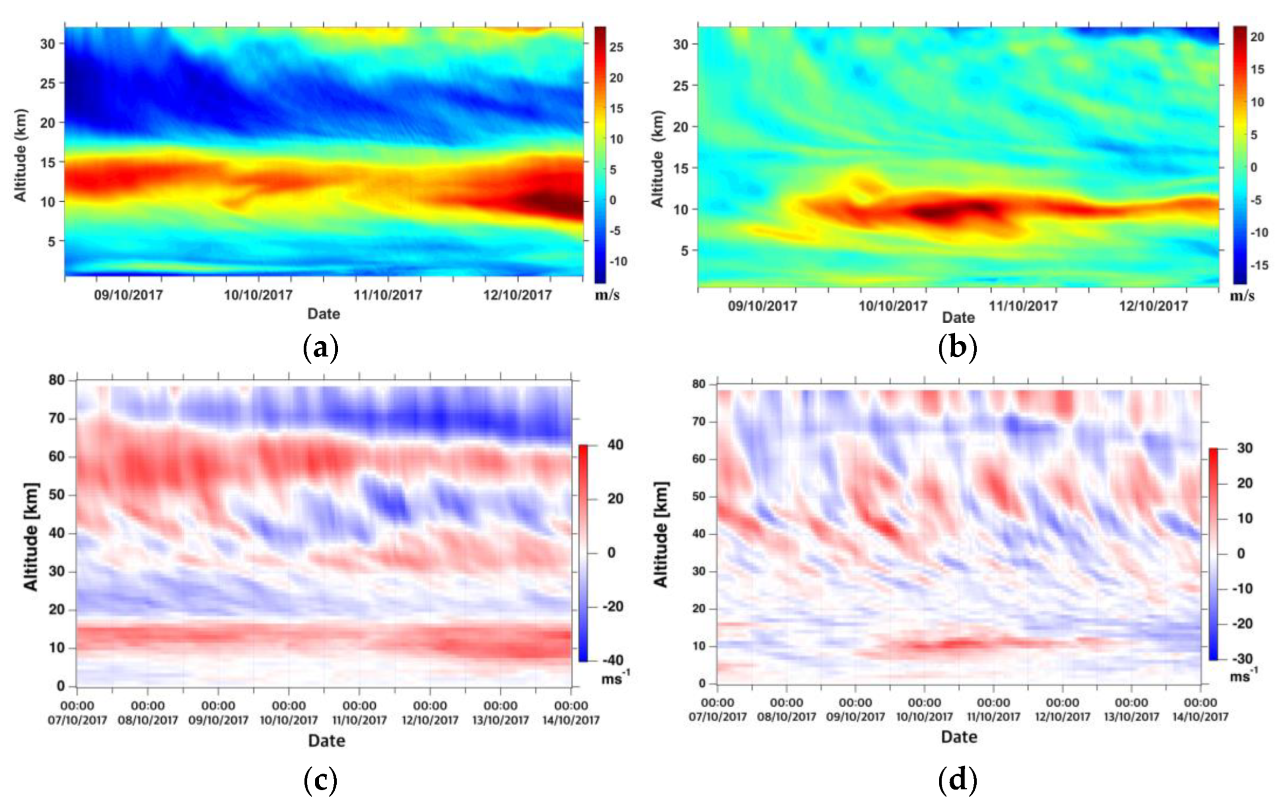
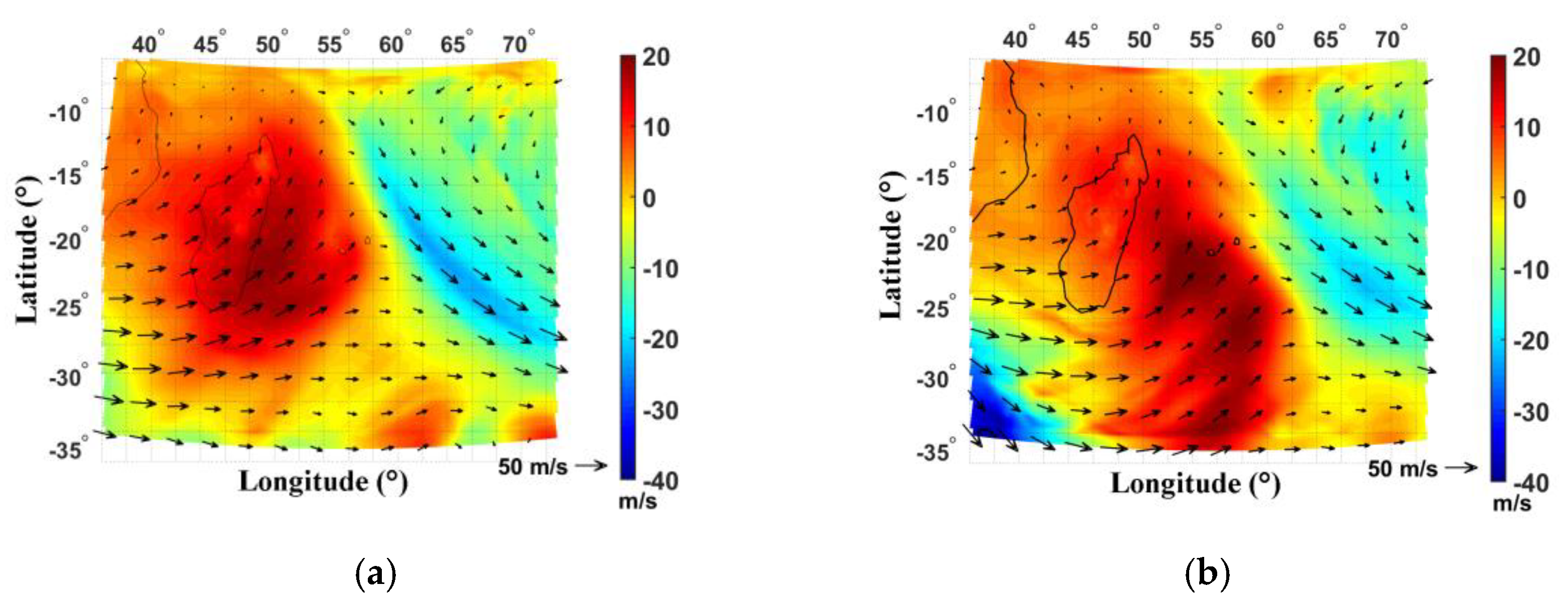
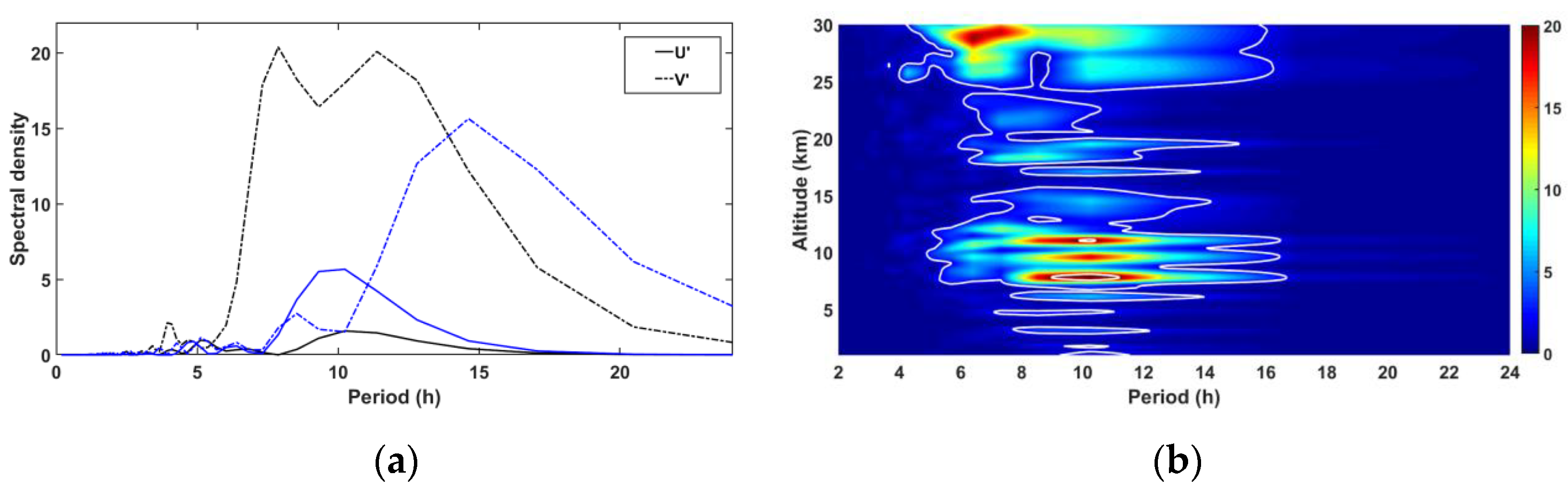
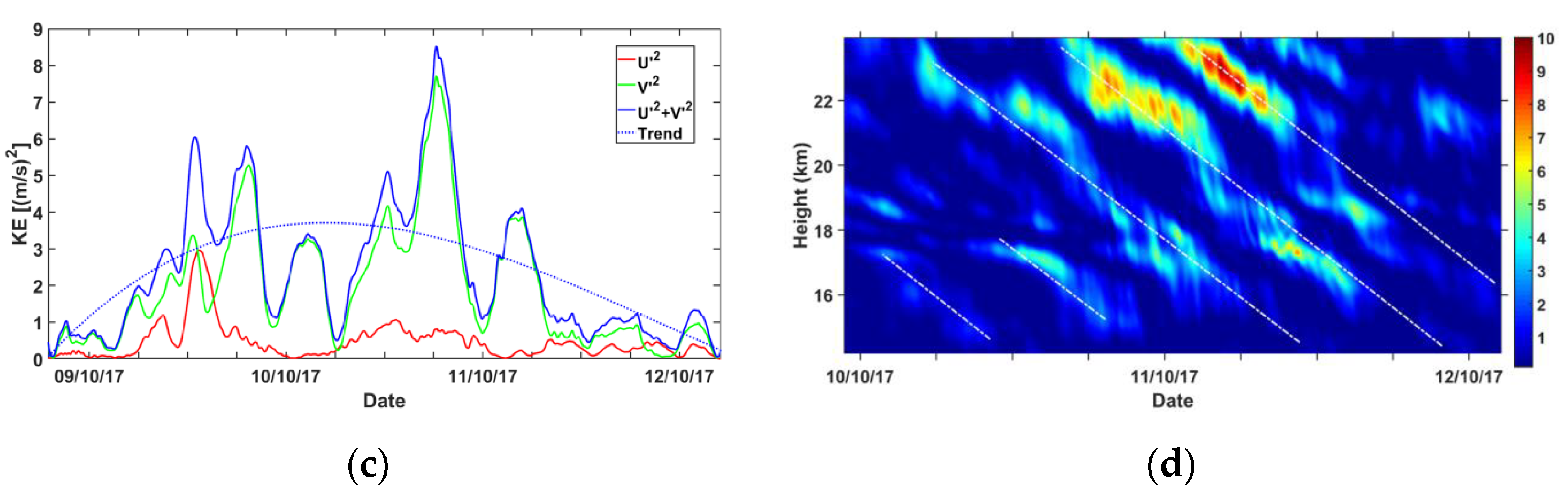
• In the lower atmosphere, both observations and weather models supported that the RWB in the middle troposphere triggers GW activity at the subtropical barrier above La Réunion on 9–12 October 2017. Radiosonde data highlighted dominant low-frequency GW modes with vertical wavelengths of about 1.5–3 km and 4–7 km, periods of 5–27 h and horizontal wavelengths between 200 km and 1300 km at heights of 18–28 km with a dominant south-eastward horizontal propagation. High-resolution mesoscale modeling provided a fine description of the meteorological event and supported observations about GW characteristics in the lower atmosphere. The activity of GW kinetic energy near the source varied with periods of 5–10 h. Dominant GWs with vertical wavelengths of 2–3 km and ~ 6 km were clearly identified during their upward propagation from the source up to the stratosphere on 9–11 October. Mesoscale modeling and ray tracing also confirmed the important role of RWB for GW activity at the southern subtropical latitudes [75] and also upward wave propagation of tropospheric GW modes into the mesosphere. In particular, dominant mesospheric GW modes with vertical wavelengths of about 4–6 km and 10–13 km were traced down to the troposphere and up to the mesopause.
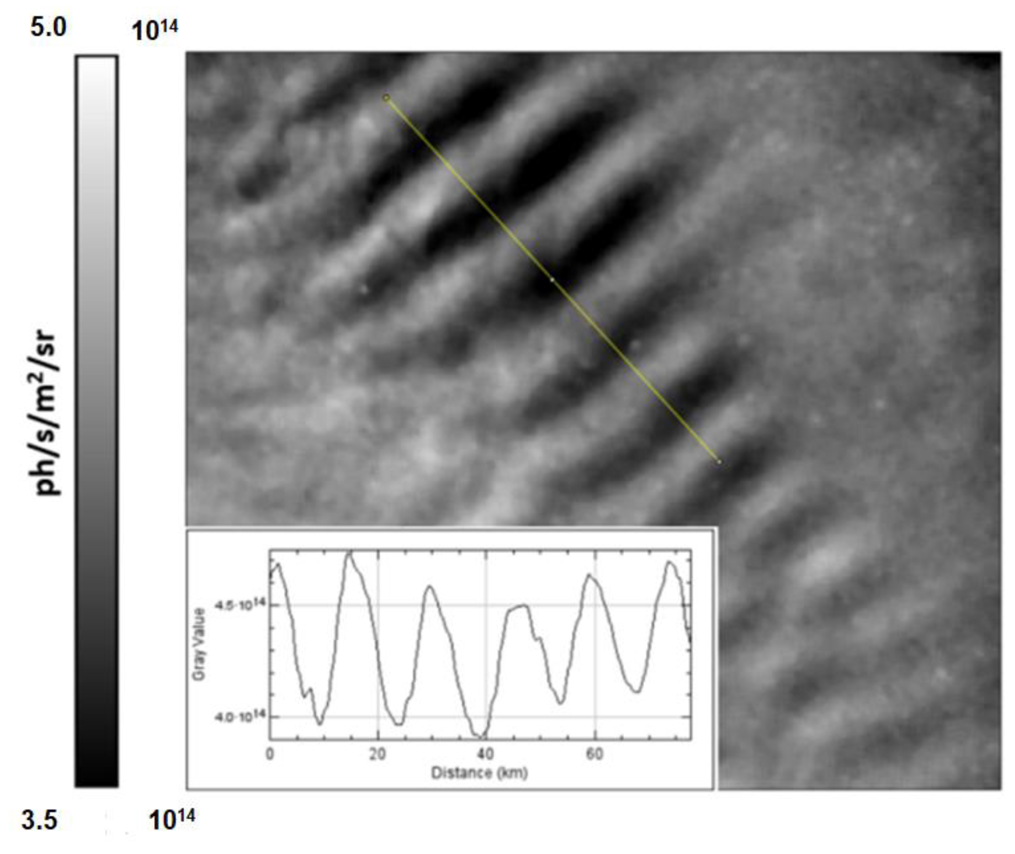
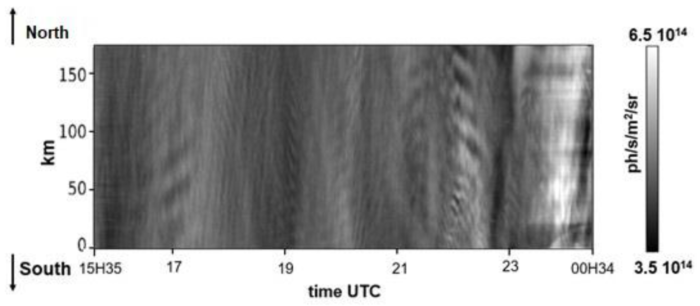
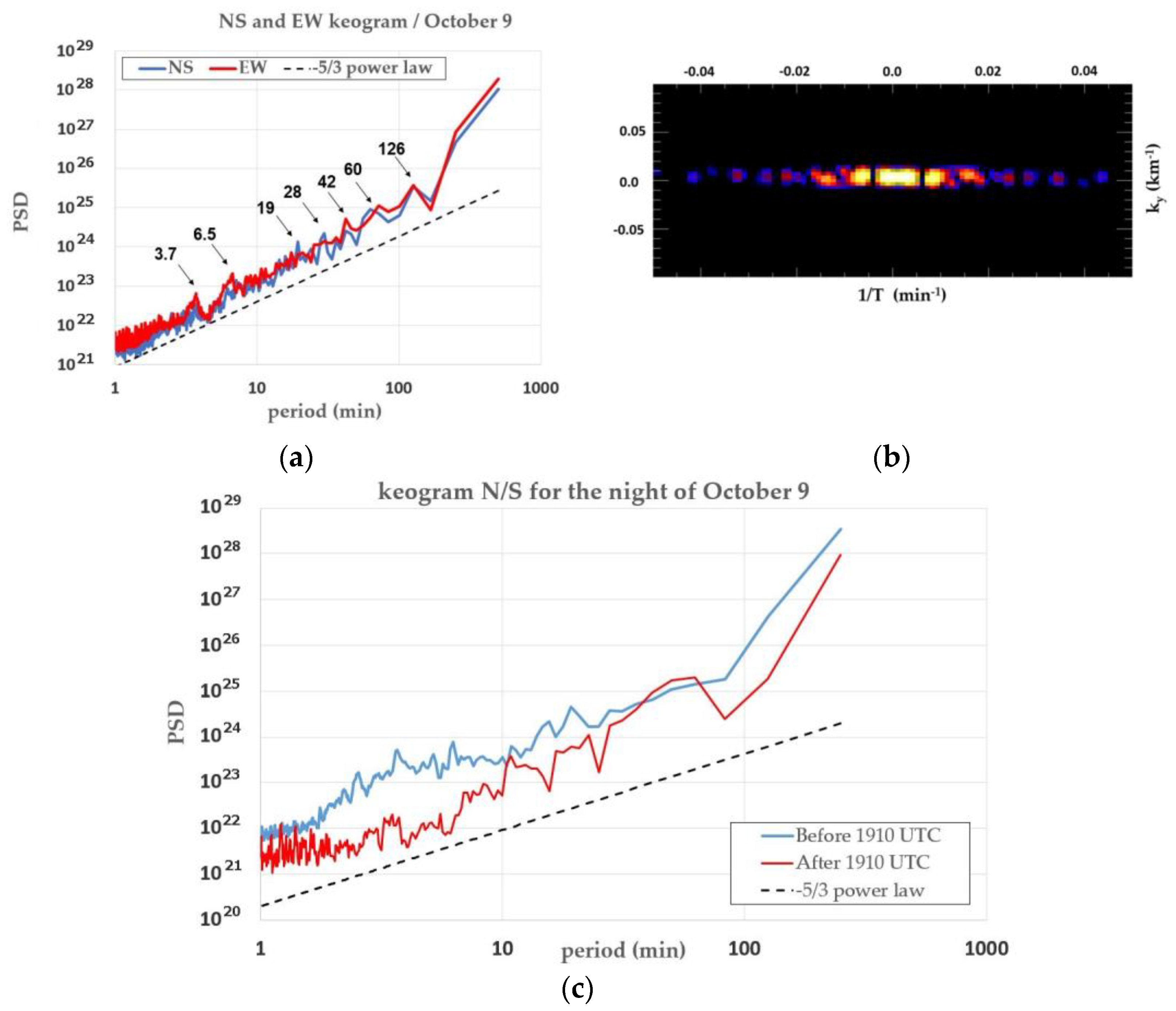
• In the upper mesosphere—mesopause, strong GW activity was also reported in SABER data on 9–11 October 2017 in the vicinity of La Réunion. Breaking waves were observed below the MIL and in the mesopause. Shorter and broader range wavelengths are observed in the mesopause in comparison with the upper mesosphere, probably because of the generation of secondary GWs due to breaking waves. A dominant GW with a vertical wavelength of 4–5 km was clearly visualized in the mesosphere up to 100 km in height in the lower thermosphere. At the OH layer around 87 km in height, several techniques were developed to extract spectral characteristics for high and low-frequency GWs using nightglow images on both nights. Modes with short periods of between 3.3 min and 2.1 h and horizontal wavelengths of 8–17 km on 9–10 October detected in the mesopause might be attributed to secondary waves due to wave breaking. The periodogram of the keograms identified a long period of about 8 h. Nightly variation of GW activity depending on GW periods was observed on nights of 9 and 10 October.

Finally, the study supports that tropospheric RWB can induce strong tropospheric GW activity at the subtropical barrier, possibly responsible for the formation of MILs during austral winter. It also provides a methodology and several techniques to improve the understanding of the link between MILs and GWs. In particular, the MRA has proven to be an effective tool for capturing GWs in observational and modeling data. Moreover, high-resolution modeling also offers the possibility of reproducing fairly well GWs in the lower atmosphere to characterize related tropospheric GW sources.

Among future research, a statistical study is needed to explore MILs and both GWs and planetary waves in the middle atmosphere and simulated MILs in climate model WACCM in the tropics. Indeed, MILs are frequently observed on Lidar observations over La Réunion [24]. Moreover, planetary wave breaking is also known as another important cause for the formation of lower MILs, which was not the case in the present study. Regarding the simulation of MILs with WACCM, France et al. [29] pointed at either a warm bias in the mesosphere or a too-large planetary wave activity to explain an overestimation of MIL occurrences within WACCM. Discrepancies between observations and modeling in the upper atmosphere are also a motivation to investigate the physical reasons and to improve climate models [1].

References

1. Lübken, F.J. Physics in the mesosphere/lower thermosphere: A personal perspective. Front. Astron. Space Sci. 2022, 9, 1000766. [Google Scholar] [CrossRef]
2. Gerber, E.P.; Butler, A.; Calvo, N.; Charlton-Perez, A.; Giorgetta, M.; Manzini, E.; Perlwitz, J.; Polvani, L.M.; Sassi, F.; Scaife, A.A.; et al. Assessing and understanding the impact of stratospheric dynamics and variability on the earth system. Bull. Am. Meteorol. Soc. 2012, 93, 845–859. [Google Scholar] [CrossRef] [Green Version]
3. Martin, Z.; Vitart, F.; Wang, S.; Sobel, A. The impact of the stratosphere on the MJO in a forecast model. J. Geophys. Res. Atmos. 2020, 125, e2019JD032106. [Google Scholar] [CrossRef]
4. Domeisen, D.I.V.; Butler, A.H.; Charlton-Perez, A.J.; Ayarzagüena, B.; Baldwin, M.P.; Dunn-Sigouin, E.; Furtado, J.C.; Garfinkel, C.I.; Hitchcock, P.; Karpechko, A.Y.; et al. The role of the stratosphere in subseasonal to seasonal prediction: 1. Predictability of the stratosphere. J. Geophys. Res. Atmos. 2020, 125, e2019JD030920. [Google Scholar] [CrossRef]
5. Garfinkel, C.I.; Gerber, E.P.; Shamir, O.; Rao, J.; Jucker, M.; White, I.; Paldor, N. A QBO cookbook: Sensitivity of the quasi-biennial oscillation to resolution, resolved waves, and parameterized gravity waves. J. Adv. Model. Earth Syst. 2022, 14, e2021MS002568. [Google Scholar] [CrossRef]
6. Yu, Y.; Cai, M.; Garfinkel, C. Editorial: Stratosphere-troposphere coupling and its role in surface weather predictability. Front. Earth Sci. 2022, 10, 478. [Google Scholar] [CrossRef]
7. Domeisen, D.I.V.; Butler, A.H.; Charlton-Perez, A.J.; Ayarzagüena, B.; Baldwin, M.P.; Dunn-Sigouin, E.; Furtado, J.C.; Garfinkel, C.I.; Hitchcock, P.; Karpechko, A.Y.; et al. The role of the stratosphere in subseasonal to seasonal prediction: 2. Predictability arising from stratosphere-troposphere coupling. J. Geophys. Res. Atmos. 2020, 125, e2019JD030923. [Google Scholar] [CrossRef]
8. Ern, M.; Hoffmann, L.; Rhode, S.; Preusse, P. The mesoscale gravity wave response to the 2022 Tonga volcanic eruption: AIRS and MLS satellite observations and source backtracing. Geophys. Res. Lett. 2022, 49, e2022GL098626. [Google Scholar] [CrossRef]
9. Hines, C.O. Internal atmospheric gravity waves at ionospheric heights. Can. J. Phys. 1960, 38, 1441–1481. [Google Scholar] [CrossRef]
10. Hines, C.O.; Adams, G.W.; Brosnahan, J.W.; Djuth, F.T.; Sulzer, M.P.; Tepley, C.A.; Van Baelen, J. Multi-instrument observations of mesospheric motions over Arecibo: Comparisons and interpretations. J. Atmos. Terr. Phys. 1993, 55, 241–287. [Google Scholar] [CrossRef]
11. Hickey, M.P.; Walterscheid, R.L.; Schubert, G. Gravity wave heating and cooling of the thermosphere: Sensible heat flux and viscous flux of kinetic energy. J. Geophys. Res. Space Phys. 2011, 116, A12326. [Google Scholar] [CrossRef] [Green Version]
12. Reichert, R.; Kaifler, B.; Kaifler, N.; Rapp, M.; Pautet, P.-D.; Taylor, M.J.; Kozlovsky, A.; Lester, M.; Kivi, R. Retrieval of intrinsic mesospheric gravity wave parameters using lidar and airglow temperature and meteor radar wind data. Atmos. Meas. Tech. 2019, 12, 5997–6015. [Google Scholar] [CrossRef] [Green Version]
13. Liu, H.L.; McInerney, J.M.; Santos, S.; Lauritzen, P.H.; Taylor, M.A.; Pedatella, N.M. Gravity waves simulated by high-resolution Whole Atmosphere Community Climate Model. Geophys. Res. Lett. 2014, 41, 9106–9112. [Google Scholar] [CrossRef] [Green Version]
14. Harvey, V.L.; Pedatella, N.; Becker, E.; Randall, C. Evaluation of polar winter mesopause wind in WACCMX+DART. J. Geophys. Res. Atmos. 2022, 127, e2022JD037063. [Google Scholar] [CrossRef]
15. Mariaccia, A.; Keckhut, P.; Hauchecorne, A.; Claud, C.; Le Pichon, A.; Meftah, M.; Khaykin, S. Assessment of ERA-5 Temperature variability in the middle atmosphere using Rayleigh lidar measurements between 2005 and 2020. Atmosphere 2022, 13, 242. [Google Scholar] [CrossRef]
16. Fritts, D.C.; Laughman, B.; Wang, L.; Lund, T.S.; Collins, R.L. Gravity wave dynamics in a mesospheric inversion layer: 1. Reflection, trapping, and instability dynamics. J. Geophys. Res. Atmos. 2018, 123, 626–648. [Google Scholar] [CrossRef] [Green Version]
17. Ardalan, M.; Keckhut, P.; Hauchecorne, A.; Wing, R.; Meftah, M.; Farhani, G. Updated Climatology of Mesospheric Temperature Inversions Detected by Rayleigh Lidar above Observatoire de Haute Provence, France, Using a K-Mean Clustering Technique. Atmosphere 2022, 13, 814. [Google Scholar] [CrossRef]
18. Hauchecorne, A.; Chanin, M.L.; Wilson, R. Mesospheric temperature inversion and gravity wave breaking. Geophys. Res. Lett. 1987, 14, 933–936. [Google Scholar] [CrossRef]
19. Wing, R.; Martic, M.; Triplett, C.; Hauchecorne, A.; Porteneuve, J.; Keckhut, P.; Courcoux, Y.; Yung, L.; Retailleau, P.; Cocuron, D. Gravity wave breaking associated with mesospheric inversion layers as measured by the Ship-Borne BEM Monge lidar and ICON-MIGHTI. Atmosphere 2021, 12, 1386. [Google Scholar] [CrossRef]
20. Yuan, T.; Pautet, P.-D.; Zhao, Y.; Cai, X.; Criddle, N.R.; Taylor, M.J.; Pendleton, W.R. Coordinated investigation of midlatitude upper mesospheric temperature inversion layers and the associated gravity wave forcing by Na lidar and Advanced Mesospheric Temperature Mapper in Logan, Utah. J. Geophys. Res. Atmos. 2014, 119, 3756–3769. [Google Scholar] [CrossRef] [Green Version]
21. Meriwether, J.W.; Gardner, C.S. A review of the mesosphere inversion layer phenomenon. J. Geophys. Res. Atmos. 2000, 105, 12405–12416. [Google Scholar] [CrossRef]
22. Liu, H.L.; Meriwether, J.W. Analysis of a temperature inversion event in the lower mesosphere. J. Geophys. Res. Atmos. 2004, 109, D02S07. [Google Scholar] [CrossRef] [Green Version]
23. Zou, X.; Yang, G.; Chen, L.; Wang, J.; Du, L. Rayleigh lidar observations and comparisons with TIMED/SABER of typical case studies in Beijing (40.5°N, 116.2°E), China. Atmosphere 2021, 12, 1237. [Google Scholar] [CrossRef]
24. Bègue, N.; Mbatha, N.; Bencherif, H.; Loua, R.T.; Sivakumar, V.; Leblanc, T. Statistical analysis of the mesospheric inversion layers over two symmetrical tropical sites: Réunion (20.8°S, 55.5°E) and Mauna Loa (19.5°N, 155.6°W). Ann. Geophys. 2017, 35, 1177–1194. [Google Scholar] [CrossRef] [Green Version]
25. Leblanc, T.; Hauchecorne, A. Recent observations of mesospheric temperature inversions. J. Geophys. Res. Atmos. 1997, 102, 19471–19482. [Google Scholar] [CrossRef] [Green Version]
26. Sassi, F.; Garcia, R.R.; Boville, B.A.; Liu, H. On temperature inversions and the mesospheric surf zone. J. Geophys. Res. Atmos. 2002, 107, 4380–4389. [Google Scholar] [CrossRef]
27. Ramesh, K.; Sridharan, S.; Vijaya Bhaskara Rao, S. Causative mechanisms for the occurrence of a triple lyered mesospheric inversion event over low latitudes. J. Geophys. Res. Space Phys. 2014, 119, 3930–3943. [Google Scholar] [CrossRef]
28. Singh, R.P.; Pallamraju, D. Mesospheric temperature inversions observed in OH and O2 rotational temperatures from Mount Abu (24.6°N, 72.8°E), India. J. Geophys. Res. Space Phys. 2018, 123, 8823–8834. [Google Scholar] [CrossRef]
29. France, J.A.; Harvey, V.L.; Randall, C.E.; Collins, R.L.; Smith, A.K.; Peck, E.D.; Fang, X. A climatology of planetary wave-driven mesospheric inversion layers in the extratropical winter. J. Geophys. Res. Atmos. 2015, 120, 399–413. [Google Scholar] [CrossRef]
30. Richter, J.H.; Garcia, R.R. On the Forcing of the mesospheric Semi-Annual Oscillation in the Whole Atmosphere Community Climate Model. Geophys. Res. Lett. 2006, 7, 925–935. [Google Scholar] [CrossRef]
31. Wheeling, K. Machine learning improves weather and climate models. Eos 2020, 101. [Google Scholar] [CrossRef]
32. Matsuoka, D.; Watanabe, S.; Sato, K.; Kawazoe, S.; Yu, W.; Easterbrook, S. Application of deep learning to estimate atmospheric gravity wave parameters in reanalysis data sets. Geophys. Res. Lett. 2020, 47, e2020GL089436. [Google Scholar] [CrossRef]
33. Espinosa, Z.I.; Sheshadri, A.; Cain, G.R.; Gerber, E.P.; DallaSanta, K.J. Machine learning gravity wave parameterization generalizes to capture the QBO and response to increased CO2. Geophys. Res. Lett. 2022, 49, e2022GL098174. [Google Scholar] [CrossRef]
34. Hindley, N.P.; Wright, C.J.; Smith, N.D.; Hoffmann, L.; Holt, L.A.; Alexander, M.J.; Moffat-Griffin, T.; Mitchell, N.J. Gravity waves in the winter stratosphere over the Southern Ocean: High-resolution satellite observations and 3-D spectral analysis. Atmos. Chem. Phys. 2019, 19, 15377–15414. [Google Scholar] [CrossRef] [Green Version]
35. Mann, A. Core concept: Nascent exascale supercomputers offer promise, present challenges. Proc. Natl. Acad. Sci. USA 2020, 117, 22623–22625. [Google Scholar] [CrossRef]
36. Chane Ming, F.; Ibrahim, C.; Barthe, C.; Jolivet, S.; Keckhut, P.; Liou, Y.A.; Kuleshov, Y. Observation and a numerical study of gravity waves during tropical cyclone Ivan (2008). Atmos. Chem. Phys. 2014, 14, 641–658. [Google Scholar] [CrossRef] [Green Version]
37. Baray, J.-L.; Courcoux, Y.; Keckhut, P.; Portafaix, T.; Tulet, P.; Cammas, J.P.; Hauchecorne, A.; Godin-Beekmann, S.; De Mazière, M.; Hermans, C.; et al. Maïdo observatory: A new high-altitude station facility at Reunion Island (21° S, 55° E) for long-term atmospheric remote sensing and in situ measurements. Atmos. Meas. Tech. 2013, 6, 2865–2877. [Google Scholar] [CrossRef] [Green Version]
38. Keckhut, P.; Courcoux, Y.; Baray, J.-L.; Porteneuve, J.; Vérèmes, H.; Hauchecorne, A.; Dionisi, D.; Posny, F.; Cammas, J.-P.; Payen, G.; et al. Introduction to the Maïdo lidar calibration campaign dedicated to the validation of upper air meteorological parameters. J. Appl. Rem. Sens. 2015, 9, 094099. [Google Scholar] [CrossRef] [Green Version]
39. Hauchecorne, A.; Chanin, M. Density and temperature profiles obtained by lidar between 35 and 70 km. Geophys. Res. Lett. 1980, 7, 565–568. [Google Scholar] [CrossRef]
40. Picone, J.M.; Hedin, A.E.; Drob, D.P.; Aikin, A.C. NRLMSISE-00 empirical model of the atmosphere: Statistical comparisons and scientific issues. J. Geophys. Res. Atmos. 2002, 107, 1468. [Google Scholar] [CrossRef]
41. Keckhut, P.; Hauchecorne, A.; Chanin, M.L. A Critical Review of the database acquired for the long-term surveillance of the middle atmosphere by the French Rayleigh lidars. J. Atmos. Ocean. Tech. 1993, 10, 850–867. [Google Scholar] [CrossRef]
42. Von Savigny, C.; McDade, I.C.; Eichmann, K.-U.; Burrows, J.P. On the dependence of the OH Meinel emission altitude on vibrational level: Sciamachy observations and model simulations. Atmos. Chem. Phys. 2012, 12, 8813–8828. [Google Scholar] [CrossRef] [Green Version]
43. Mlynczak, M.G. Energetics of the mesosphere and lower thermosphere and the SABER experiment. Adv. Space Res. 1997, 20, 1177–1183. [Google Scholar] [CrossRef]
44. Eckermann, S.D. Ray-tracing simulation of the global propagation of inertia gravity waves through the zonally averaged middle atmosphere. J. Geophys. Res. Atmos. 1992, 97, 15849–15866. [Google Scholar] [CrossRef]
45. Marks, C.J.; Eckermann, S.D. A Three-dimensional nonhydrostatic ray-tracing model for gravity waves: Formulation and preliminary results for the middle atmosphere. J. Atmos. Sci. 1995, 52, 1959–1984. [Google Scholar] [CrossRef]
46. Jones, R.M.; Bedard, A.J. Atmospheric gravity wave ray tracing: Ordinary and extraordinary waves. J. Atmos. Sol. Terr. Phys. 2018, 179, 342–357. [Google Scholar] [CrossRef]
47. Chane Ming, F.; Vignelles, D.; Jegou, F.; Berthet, G.; Renard, J.B.; Gheusi, F.; Kuleshov, Y. Gravity-wave effects on tracer gases and stratospheric aerosol concentrations during the 2013 ChArMEx campaign. Atmos. Chem. Phys. 2016, 16, 8023–8042. [Google Scholar] [CrossRef] [Green Version]
48. Pramitha, M.; Kumar, K.K.; Ratnam, M.V.; Praveen, M.; Rao, S.V.B. Gravity wave source spectra appropriation for mesosphere lower thermosphere using meteor radar observations and GROGRAT model simulations. Geophys. Res. Lett. 2020, 47, e2020GL089390. [Google Scholar] [CrossRef]
49. Perrett, J.A.; Wright, C.J.; Hindley, N.P.; Hoffmann, L.; Mitchell, N.J.; Preusse, P.; Strube, C.; Eckermann, S.D. Determining gravity wave sources and propagation in the Southern Hemisphere by ray-tracing AIRS measurements. Geophys. Res. Lett. 2021, 48, e2020GL088621. [Google Scholar] [CrossRef]
50. Strube, C.; Preusse, P.; Ern, M.; Riese, M. Propagation paths and source distributions of resolved gravity waves in ECMWF-IFS analysis fields around the southern polar night jet. Atmos. Chem. Phys. 2021, 21, 18641–18668. [Google Scholar] [CrossRef]
51. Preusse, P.; Eckermann, S.D.; Ern, M.; Oberheide, J.; Picard, R.H.; Roble, R.G.; Riese, M.; Russell, J.M.; Mlynczak, M.G. Global ray tracing simulations of the SABER gravity wave climatology. J. Geophys. Res. Atmos. 2009, 114, D08126. [Google Scholar] [CrossRef]
52. Amemiya, A.; Sato, K. A New Gravity wave parameterization including three-dimensional propagation. J. Meteor. Soc. Japan. Ser. II 2016, 94, 237–256. [Google Scholar] [CrossRef] [Green Version]
53. Song, I.-S.; Lee, C.; Chun, H.-Y.; Kim, J.-H.; Jee, G.; Song, B.-G.; Bacmeister, J.T. Propagation of gravity waves and its effects on pseudomomentum flux in a sudden stratospheric warming event. Atmos. Chem. Phys. 2020, 20, 7617–7644. [Google Scholar] [CrossRef]
54. Tidiga, M.; Berthet, G.; Jégou, F.; Kloss, C.; Bègue, N.; Vernier, J.-P.; Renard, J.-B.; Bossolasco, A.; Clarisse, L.; Taha, G.; et al. Variability of the aerosol content in the tropical lower stratosphere from 2013 to 2019: Evidence of volcanic eruption impacts. Atmosphere 2022, 13, 250. [Google Scholar] [CrossRef]
55. Hersbach, H.; Bell, B.; Berrisford, P.; Hirahara, S.; Horanyi, A.; Muñoz-Sabater, J.; Nicolas, J.; Peubey, C.; Radu, R.; Schepers, D.; et al. The ERA5 global reanalysis. Q. J. R. Meteorol. Soc. 2020, 146, 1999–2049. [Google Scholar] [CrossRef]
56. Gupta, A.; Birner, T.; Dörnbrack, A.; Polichtchouk, I. Importance of gravity wave forcing for springtime southern polar vortex breakdown as revealed by ERA5. Geophys. Res. Lett. 2021, 48, e2021GL092762. [Google Scholar] [CrossRef]
57. Pahlavan, H.A.; Fu, Q.; Wallace, J.M.; Kiladis, G.N. Revisiting the Quasi-Biennial Oscillation as seen in ERA5. Part I: Description and momentum budget. J. Atmos. Sci. 2021, 78, 673–691. [Google Scholar] [CrossRef]
58. Pahlavan, H.A.; Wallace, J.M.; Fu, Q. Characteristics of convectively generated gravity waves resolved by ERA5 reanalysis. Earth Space Sci. Open Arch. 2022, 20, 1–25. [Google Scholar] [CrossRef]
59. Jewtoukoff, V.; Hertzog, A.; Plougonven, R.; de al Cámara, A.; Lott, F. Comparison of gravity waves in the Southern Hemisphere derived from balloon observations and the ECMWF analyses. J. Atmos. Sci. 2015, 72, 3449–3468. [Google Scholar] [CrossRef]
60. Powers, J.G.; Klemp, J.B.; Skamarock, W.C.; Davis, C.A.; Dudhia, J.; Gill, D.O.; Coen, J.L.; Gochis, D.J.; Ahmadov, R.; Peckham, S.E.; et al. The Weather Research and Forecasting model: Overview, system efforts, and future directions. Bull. Am. Meteor. Soc. 2017, 98, 1717–1737. [Google Scholar] [CrossRef]
61. Tridon, F.; Planche, C.; Mroz, K.; Banson, S.; Battaglia, A.; Van Baelen, J.; Wobrock, W. On the realism of the rain microphysics representation of a squall line in the WRF model. Part I: Evaluation with multifrequency radar Doppler spectra observations. Mon. Weather Rev. 2019, 147, 2787–2810. [Google Scholar] [CrossRef] [Green Version]
62. Plougonven, R.; Hertzog, A.; Guez, L. Gravity waves over antarctica and the southern ocean: Consistent momentum fluxes in mesoscale simulations and stratospheric balloon observations. Atmosphere 2013, 4, 485–505. [Google Scholar] [CrossRef]
63. Hima Bindu, H.; Venkat Ratnam, M.; Viswanadhapalli, Y.; Hari Prasad, D. Medium frequency gravity wave characteristics obtained using Weather Research and Forecasting (WRF) model simulations. J. Atmos. Sol. Terr. Phys. 2019, 182, 119–129. [Google Scholar] [CrossRef]
64. Chane Ming, F.; Jolivet, S.; Liou, Y.-A.; Jégou, F.; Mekies, D.; Hong, J.-S. Elliptical structures of gravity waves produced by typhoon Soudelor in 2015 near Taiwan. Atmosphere 2019, 10, 260. [Google Scholar] [CrossRef] [Green Version]
65. Drob, D.P.; Emmert, J.T.; Meriwether, J.W.; Makela, J.J.; Doornbos, E.; Conde, M.; Hernandez, G.; Noto, J.; Zawdie, K.A.; McDonald, S.E.; et al. An update to the Horizontal Wind Model (HWM): The quiet time thermosphere. Earth Space Sci. 2015, 2, 301–319. [Google Scholar] [CrossRef]
66. Paulino, I.; Figueiredo, C.A.O.B.; Rodrigues, F.S.; Buriti, R.A.; Wrasse, C.M.; Paulino, A.R.; Barros, D.; Takahashi, H.; Batista, I.S.; Medeiros, A.F.; et al. Atmospheric gravity waves observed in the nightglow following the 21 August 2017 total solar eclipse. Geophys. Res. Lett. 2020, 47, e2020GL088924. [Google Scholar] [CrossRef]
67. Takahashi, H.; Figueiredo, C.A.O.B.; Essien, P.; Wrasse, C.M.; Barros, D.; Nyassor, P.K.; Paulino, I.; Egito, F.; Rosa, G.M.; Sampaio, A.H.R. Signature of gravity wave propagations from the troposphere to ionosphere. Ann. Geophys. 2022, 40, 665–672. [Google Scholar] [CrossRef]
68. Mzé, N.; Hauchecorne, A.; Keckhut, P.; Thétis, M. Vertical distribution of gravity wave potential energy from long-term Rayleigh lidar data at a northern middle-latitude site. J. Geophys. Res. Atmos. 2014, 119, 12069–12083. [Google Scholar] [CrossRef]
69. Chane Ming, F.; Molinaro, F.; Leveau, J.; Keckhut, P.; Hauchecorne, A. Analysis of gravity waves in the tropical middle atmosphere over La Reunion Island (21°S, 55°E) with lidar using wavelet techniques. Ann. Geophys. 2000, 18, 485–498. [Google Scholar] [CrossRef] [Green Version]
70. Chane Ming, F.; Molinaro, F.; Leveau, J.; Keckhut, P.; Hauchecorne, A.; Godin, S. Vertical short-scale structures in the upper tropospheric and lower stratospheric temperature and ozone at la Réunion Island (20.8°S 55.3°E). J. Geophys. Res. Atmos. 2000, 105, 485–498. [Google Scholar] [CrossRef] [Green Version]
71. Bageston, J.V.; Wrasse, C.M.; Figueiredo, C.; Giongo, G.A.; Takahashi, H.; Gobbi, D.; Leme, N.M.P. Mesospheric gravity waves observed over Ferraz station and future plan. In Proceedings of the 3rd International ANtarctic Gravity Wave Instrument Network (ANGWIN) Science Workshop, Cambridge, UK, 12 April 2016. [Google Scholar]
72. Klekociuk, A.R.; Tully, M.B.; Krummel, P.B.; Evtushevsky, O.; Kravchenko, V.; Henderson, S.I.; Alexander, S.P.; Querel, R.R.; Nichol, S.E.; Smale, D.A.; et al. The Antarctic ozone hole during 2017. J. South. Hemisph. Earth Syst. Sci. 2019, 69, 29–51. [Google Scholar] [CrossRef]
73. Evtushevsky, O.; Klekociuk, A.R.; Kravchenko, V.; Milinevsky, G.P.; Grytsai, A. The influence of large amplitude planetary waves on the Antarctic ozone hole of austral spring 2017. J. South. Hemisph. Earth Syst. Sci. 2019, 69, 57–64. [Google Scholar] [CrossRef]
74. Serafimovich, A.; Hoffmann, P.; Peters, D.; Lehmann, V. Investigation of inertia-gravity waves in the upper troposphere/lower stratosphere over Northern Germany observed with collocated VHF/UHF radars. Atmos. Chem. Phys. 2005, 5, 295–310. [Google Scholar] [CrossRef] [Green Version]
75. Zülicke, C.; Peters, D. Simulation of Inertia–Gravity Waves in a Poleward-Breaking Rossby Wave. J. Atmos. Sci. 2006, 63, 3253–3276. [Google Scholar] [CrossRef]
76. Peters, D.; Waugh, D.W. Rossby wave breaking in the southern hemisphere wintertime upper troposphere. Mon. Weather Rev. 2003, 131, 2623–2634. [Google Scholar] [CrossRef]
77. Plougonven, R.; Zhang, F. Internal gravity waves from atmospheric jets and fronts. Atmosphere 2014, 5, 1657–1689. [Google Scholar] [CrossRef] [Green Version]
78. Homeyer, C.R.; Bowman, K.P. Rossby wave breaking and transport between the tropics and extratropics above the subtropical jet. J. Atmos. Sci. 2013, 70, 607–626. [Google Scholar] [CrossRef] [Green Version]
79. Ndarana, T.; Waugh, D.W. A Climatology of Rossby Wave Breaking on the Southern Hemisphere Tropopause. J. Atmos. Sci. 2011, 68, 798–811. [Google Scholar] [CrossRef] [Green Version]
80. Smith, S.A.; Fritts, D.C.; Vanzandt, T.E. Evidence for a saturated spectrum of atmospheric gravity waves. J. Atmos. Sci. 1987, 44, 1404–1410. [Google Scholar] [CrossRef]
81. Chane Ming, F.; Chen, Z.; Roux, F. Analysis of gravity-waves produced by intense tropical cyclones. Ann. Geophys. 2010, 28, 531–547. [Google Scholar] [CrossRef] [Green Version]
82. Vincent, R.A.; Allen, S.J.; Eckermann, S.D. Gravity-wave parameters in the lower stratosphere. In Gravity Wave Processes; Hamilton, K., Ed.; Springer: Berlin/Heidelberg, Germany, 1997; pp. 7–25. [Google Scholar] [CrossRef]
83. Bellisario, C. Modélisation du Rayonnement Proche Infrarouge Émis par la Haute Atmosphère: Étude Théorique et Observationnelle. Chapter 4. Ph.D. Thesis, Université Paris-Saclay, Gif-sur-Yvette, France, 2015. [Google Scholar]
84. Le Du, T.; Keckhut, P.; Hauchecorne, A.; Simoneau, P. Observation of gravity wave vertical propagation through a mesospheric inversion layer. Atmosphere 2022, 13, 1003. [Google Scholar] [CrossRef]
85. Tang, J.; Kamalabadi, F.; Franke, S.; Liu, A.; Swenson, G. Estimation of gravity wave momentum flux with spectroscopic imaging. IEEE Trans. Geosci. Remote Sens. 2005, 43, 103–109. [Google Scholar] [CrossRef]
86. Vargas, F.; Fuentes, J.; Vega, P.; Navarro, L.; Swenson, G. Probing the analytical cancellation factor of short scale gravity waves using Na lidar and nightglow data from the Andes lidar observatory. Atmosphere 2020, 11, 1311. [Google Scholar] [CrossRef]
Figure 1. Vertical profiles of temperature (left panel), horizontal wind (right panel, zonal wind in blue, meridional wind in red) on (a) 8 October, (b) 9 October, (c) 10 October and (d) 11 October 2017 from radiosonde measurements at La Réunion (RS RUN).
Remotesensing 15 02045 g001
Figure 2. Temperature (K), zonal (m/s), meridional wind (m/s) on 9 October 2017 at ≈10.5 km height derived from WACCM (a,c,e), respectively, at 1200 UTC and from ERA5 with 137 levels (b,d,f) at 1100 UTC.
Remotesensing 15 02045 g002
Figure 3. Meridional (a) and zonal (b) wind from HWM14 during 9–11 October 2017 above the Maïdo observatory.
Remotesensing 15 02045 g003
Figure 4. (a) The level 6 DWT filter bank with the db8 wavelet. The normalized frequency of 0.5 is twice the vertical resolution, i.e., 300 m for lidar profiles; (b) DWT decomposition of the 15 min temperature perturbation profile at 1535 UTC (1935 LST) on 9 October 2017.
Remotesensing 15 02045 g004
Figure 5. WRF simulation from 8 October at 0600 UTC to 12 October at 1200 UTC 2017: (a) Nested domains with horizontal grid spacing of 27 km (D1), 9 km (D2) and 3 km (D3); Wind intensity (color) and wind direction (arrows) at 10 km height derived from domain D1 on (b) 8 October 0600 UTC, (c) 9 October 1200 UTC, (d) 10 October 0000 UTC, (e) 10 October 1200 UTC and (f) 11 October 0000 UTC. The length of arrows indicates the wind intensity.
Remotesensing 15 02045 g005
Figure 6. Retrieval of GW horizontal wavelength with ImageJ from GW patterns observed on a corrected radiance nightglow image (photons/s/m2/sr) on the night of 10 October 2017 at 2209 UTC. Bottom left, the intensity profile along the yellow line gives approximately a horizontal wavelength of 13 km between two peaks of intensity.
Remotesensing 15 02045 g006
Figure 7. N/S keogram on the night of 10 October 2017.
Remotesensing 15 02045 g007
Figure 8. Lidar vertical profiles of temperature on (a) 9 October from 1531 UTC to 2043 UTC and on (b) 10 October 2017 from 1628 UTC to 2112 UTC. The black solid line represents the nightly mean profile and the green shading the statistical uncertainty (±1 standard deviation). The red dashed line indicates the NRLMSISE-00 profile for comparison. (c) Hourly temperature profiles on 9 October. Successive profiles are plotted with an offset of 50 K.
Remotesensing 15 02045 g008
Figure 9. Spatial extension of the inversion feature: (a) Vertical temperature profiles extracted from WACCM simulations above La Réunion (black solid line) and where the temperature gradient is maximum “maxgrad” at 79 km height (black dashed line) within ± 10° around La Réunion on 9 October 2017. The red line refers to the smoothed lidar profiles during the corresponding night, shown at a 5 km vertical resolution; (b) Temperature gradient maps at 79 km altitude showing the location of the inversion layer. The red cross and the black square locate La Réunion and the profile “maxgrad”, respectively.
Remotesensing 15 02045 g009
Figure 10. Spectral lines for the CWT maxima with values >5% of the maximum CWT-coefficient absolute value derived from 15 min lidar temperature perturbation profiles on (a) 9 October at 1835 UTC (2235 LST) and (b) 10 October at 1645 UTC (2045 LST); Height-time variation of perturbations on 9 October with vertical wavelengths (c) >5 km and of (d) 9.6–19.2 km.
Remotesensing 15 02045 g010
Figure 11. Vertical profile of GW-EP derived from lidar temperature profiles on 9 and 10 October 2017. Solid lines represent the estimated GW-EP and the shaded areas the statistical uncertainty (±1 standard deviation). The dashed curve indicates the exponential increase in GW-EP expected without dissipation.
Remotesensing 15 02045 g011
Figure 12. (a) Wind intensity derived from WACCM at 11 km height at 1200 UTC on 9 October 2017. Contours highlight zonal wind (dashed red), meridional wind (white), wind intensity (cyan) in m/s and temperature in K (green). Heating is located above La Réunion; (b) Distribution of zonal wind and isocontours in October 2017 from radiosonde data. Black crosses on the time axis indicate available radiosounding profile and red crosses locate days 9 and 10 October; (c) Latitude–height distribution of zonal wind at longitude of 55.5°E on 9 October at 1200 UTC during austral winter derived from ERA5 (137 levels). The broken red circle locates the RWB; (d) Meteosat 8 IR image (gray levels) on 10 October 2017 at 1100 UTC and the locations of the jet (yellow arrows), the tropospheric trough and the tropical disturbance (Météo-France).
Remotesensing 15 02045 g012
Figure 13. Vertical profiles of horizontal wind perturbations on (a) 9 and (b) 10 October 2017. Spectral lines resulted from the CWT maxima with values > 15% of the maximum CWT-coefficient absolute value for (c) the zonal wind perturbations on 9 October and (d) meridional wind perturbations on 10 October. (e) Filtered horizontal wind perturbations on 10 October 2017 with a pass-band filter with cutoff wavelengths of 3–7 km and (f) hodograph of horizontal wind at heights of 18.6–23.1 km. Blue and red dots indicate the lower altitude at 18.6 km height and vertical step of 100 m, respectively.
Remotesensing 15 02045 g013
Figure 14. (a) Fourier spectral density of radiosounding (RS) filtered zonal and meridional wind perturbations (gray dashed line and black solid line, respectively) for vertical wavelengths < 7 km at heights of 18–28 km on 10 October 2017; (b) mean vertical-wavenumber power spectrum of normalized temperature perturbations (solid line) and the saturation limit [80] expressed as a function of vertical wavenumber m−3 (dashed line); and (c) angular distribution of dominant direction of horizontal propagation. Similar to Figure 4 in [82].
Remotesensing 15 02045 g014
Figure 15. Time–height distribution of zonal (left) and meridional wind (right) expressed in m/s above La Réunion derived from (a,b) WRF 6 min outputs and (c,d) hourly ERA5 dataset.
Remotesensing 15 02045 g015
Figure 16. Meridional wind intensity (m/s) and wind direction (arrows) at 10 km height on (a) 9 October at 1200 UTC, (b) 10 October 0600 UTC; Longitudinal cross sections of meridional wind intensity (m/s) along the latitude of 21°S on (c) 9 October at 1200 UTC and (d) 10 October 0600 UTC. The northward and southward jets at 10 km height are colored in red and blue, respectively, with white contours.
Remotesensing 15 02045 g016aRemotesensing 15 02045 g016b
Figure 17. (a) Same as Figure 16c but for MRA components d3 + d4 + d7 + a7; (b) fourier spectral densities of meridional wind perturbations on 9 and 10 October at 1200 UTC at heights of 5–27 km at longitudes between 52°E and 54°E; (c) hodograph of filtered simulated horizontal wind perturbations on 9 October at 1200 UTC (17–20.5 km) above Reunion (21°S, 55°E); height–longitude distributions of meridional perturbations at 21°S (d) 0.8–3.2 km (d3 + d4) and (e) 3.2–6.4 km (d5). (f) Same as (e) but with vertical wavelengths of 4–16 km superposed on the background wind using ERA5 data.
Remotesensing 15 02045 g017
Figure 18. (a) Density spectral of 6 min zonal and meridional wind perturbations (U’ and V’) from 9 October 0000 UTC to 10 October 0300 UTC (black lines) and from 10 October 0000 UTC to 11 October 0300 UTC (blue line) at 11 km height for periods < 24 h; (b) mean density spectral of zonal and meridional wind perturbations as a function of the altitude; (c) time evolution of the mean kinetic energy (KE) in the zonal (U’2) and meridional (V’2) winds as well as the total one (KE = U’2 + V’2) at heights of 8–11 km from 9 October 0000 UTC to 12 October 1200 UTC. The dotted blue line is the trend of KE; (d) time–height distribution of the kinetic energy in the meridional wind (V’2) at heights of 14–24 km. Dotted white lines highlight structures of GWs with downward phase progression.
Remotesensing 15 02045 g018aRemotesensing 15 02045 g018b
Figure 19. (a) Backward trajectories of ~90 individual modes from 9 October 2017 at 1200 UTC using ERA5 data with 37-pressure levels; (b) altitude–horizontal distribution; (c) altitude–ω/f distribution; and (d) Meteosat 8 IR image (gray levels) on 9 October 2017 at 1100 UTC.
Remotesensing 15 02045 g019
Figure 20. Forward trajectories of 90 individual modes from 9 October 2017 at 1200 UTC using ERA5 data with 137 model levels in 1D run on the vertical propagation only: (a) Altitude–vertical wavelength distribution, (b) altitude–horizontal wavelength distribution and (c) altitude–ω/f distribution.
Remotesensing 15 02045 g020
Figure 21. (a) SABER profiles from 9 October 2017 at 1455 UTC to 11 October 2017 at 2223 UTC in the region of the study. Stars mark the tangent point corresponding to an altitude of 87 km; In gray, (b) temperature (left panel) and OH VER (right panel) at 1.6 μm profiles corresponding to Figure 21a. Solid black lines show the profiles (orbit 85851) on 9 October 2017 at 1459 UTC; Fifth-order MRA applied to vertical temperature at heights of (c) 57–73 km in the upper mesosphere and (d) 77–96 km in the mesopause—lower thermosphere. From left to right, panels represent the vertical temperature profile (blue) and the linear trend (red), the temperature perturbations T’, the five details and the approximation a5.
Remotesensing 15 02045 g021
Figure 22. Time evolution of the mean radiance on the nights of 9 and 10 October 2017.
Remotesensing 15 02045 g022
Figure 23. (a) Power spectral density (PSD) of the N/S (blue) and W/E (red) keograms for the night of 9 October. The black dashed line shows the −5/3 power law; (b) Periodogram for the N/S keogram for the shortest wavenumbers. T represents the period, the ordinate the horizontal wavenumber; (c) Same as (a) but before (blue) and after (red) 1910 UTC.
Remotesensing 15 02045 g023
Figure 24. (a) Power spectral density (PSD) of the N/S (blue) and W/E (red) keograms for the night of 10 October. The black dashed line shows the −5/3 power law; (b) Periodogram for the N/S keogram for the shortest wavenumbers.
Remotesensing 15 02045 g024