


Statistical Assessments of InSAR Tropospheric Corrections: Applicability and Limitations of Weather Model Products and Spatiotemporal Filtering

Abstract
:1. Introduction
2. Materials
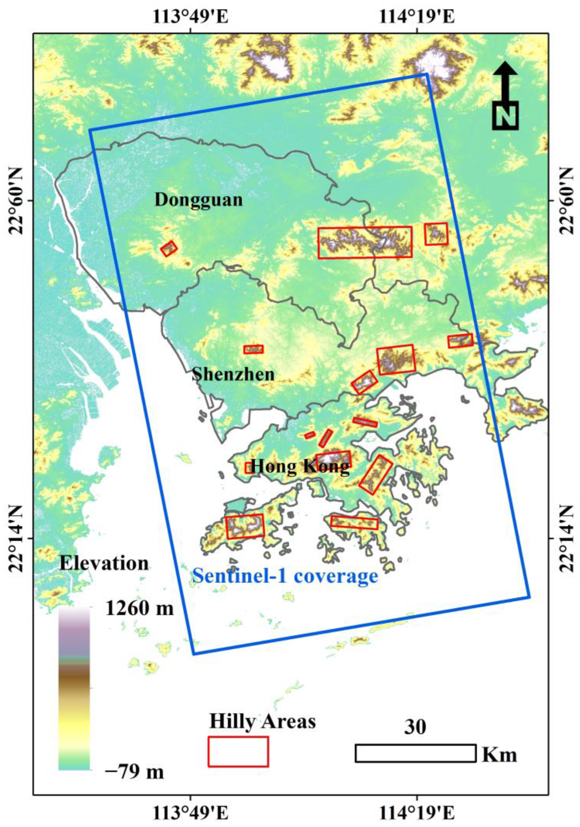
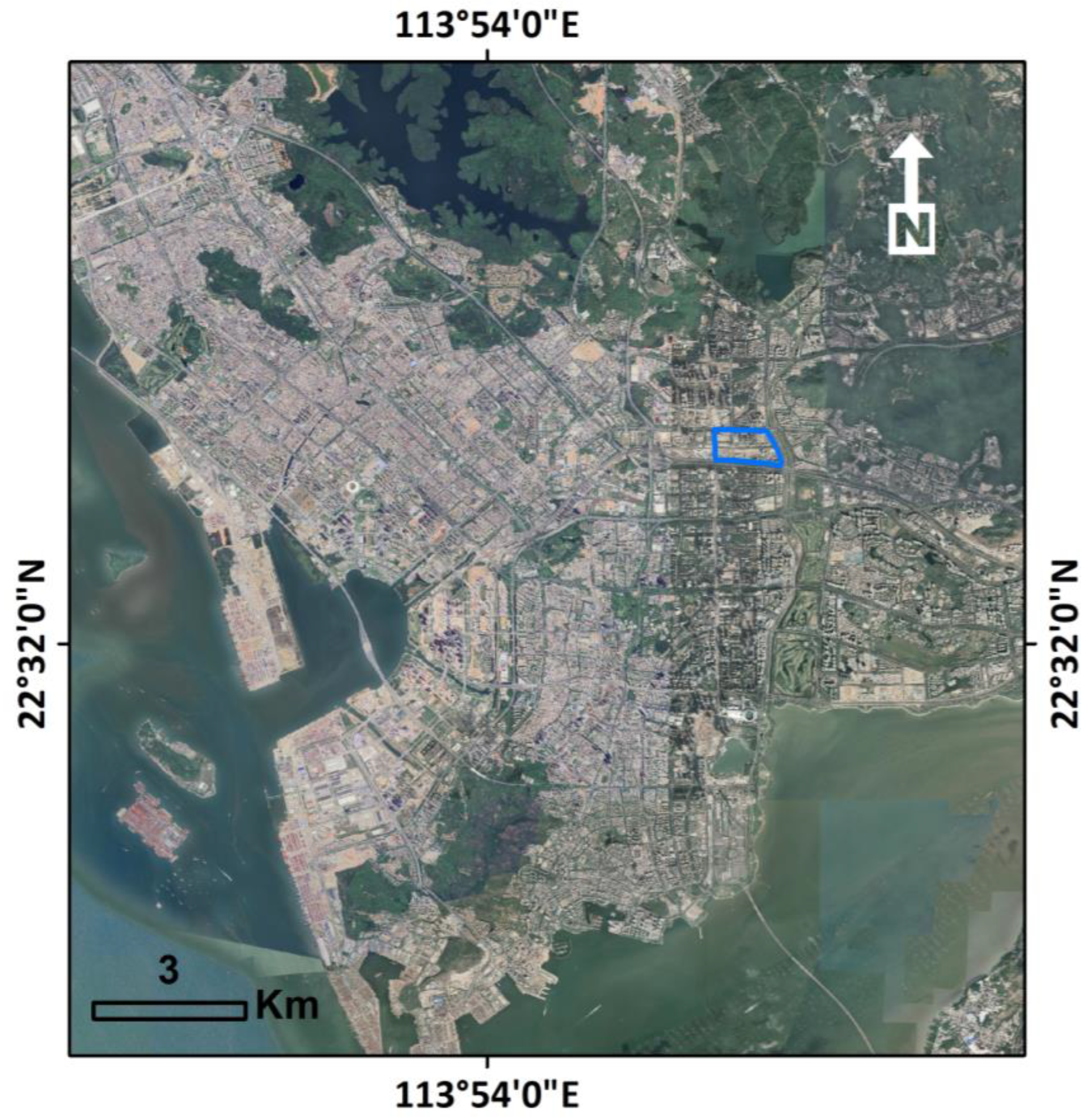
2.1. Study Area
2.2. Data
2.2.1. Sentinel-1 SAR Imagery
2.2.2. Digital Elevation Model (DEM)
2.2.3. Weather Model Products
3. Methods
3.1. Evaluation Metrics for InSAR Tropospheric Correction
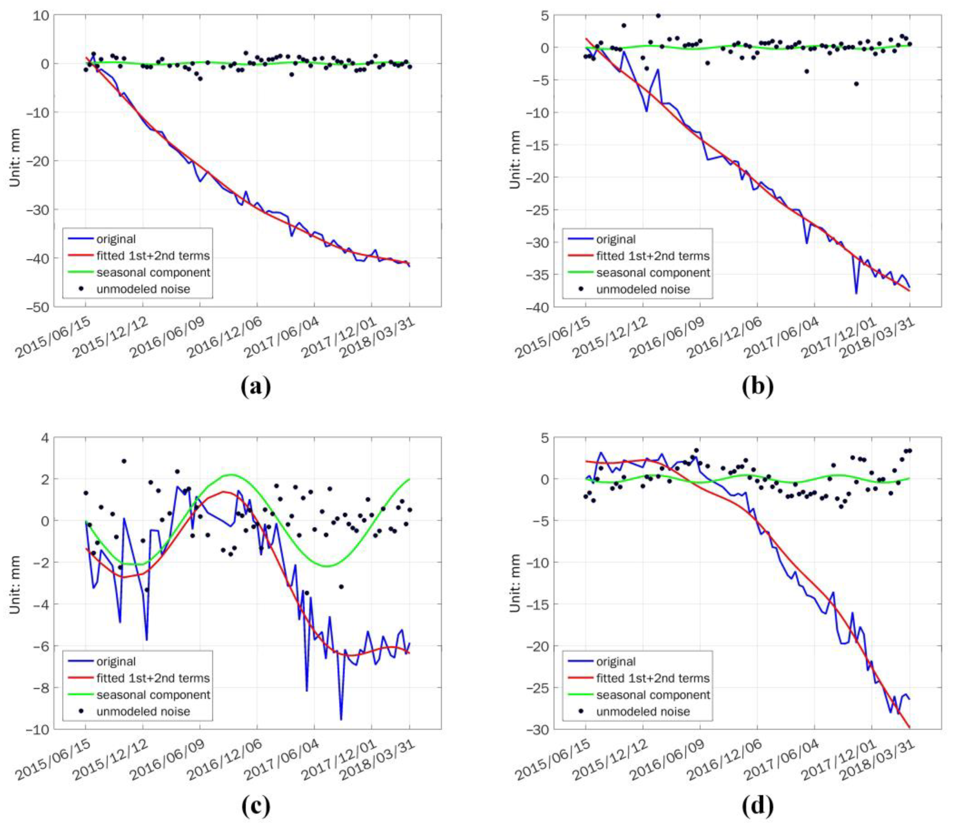
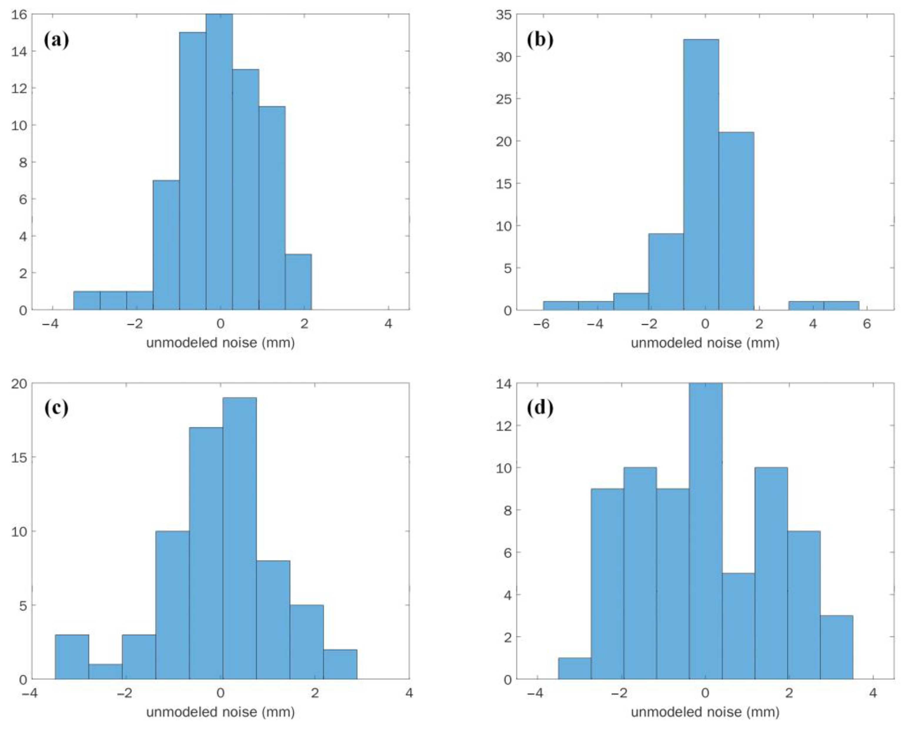
3.1.1. Tropospheric Noise Estimated by Time Series Decomposition
3.1.2. Semi-Variograms with Model Fitted Range and Sill
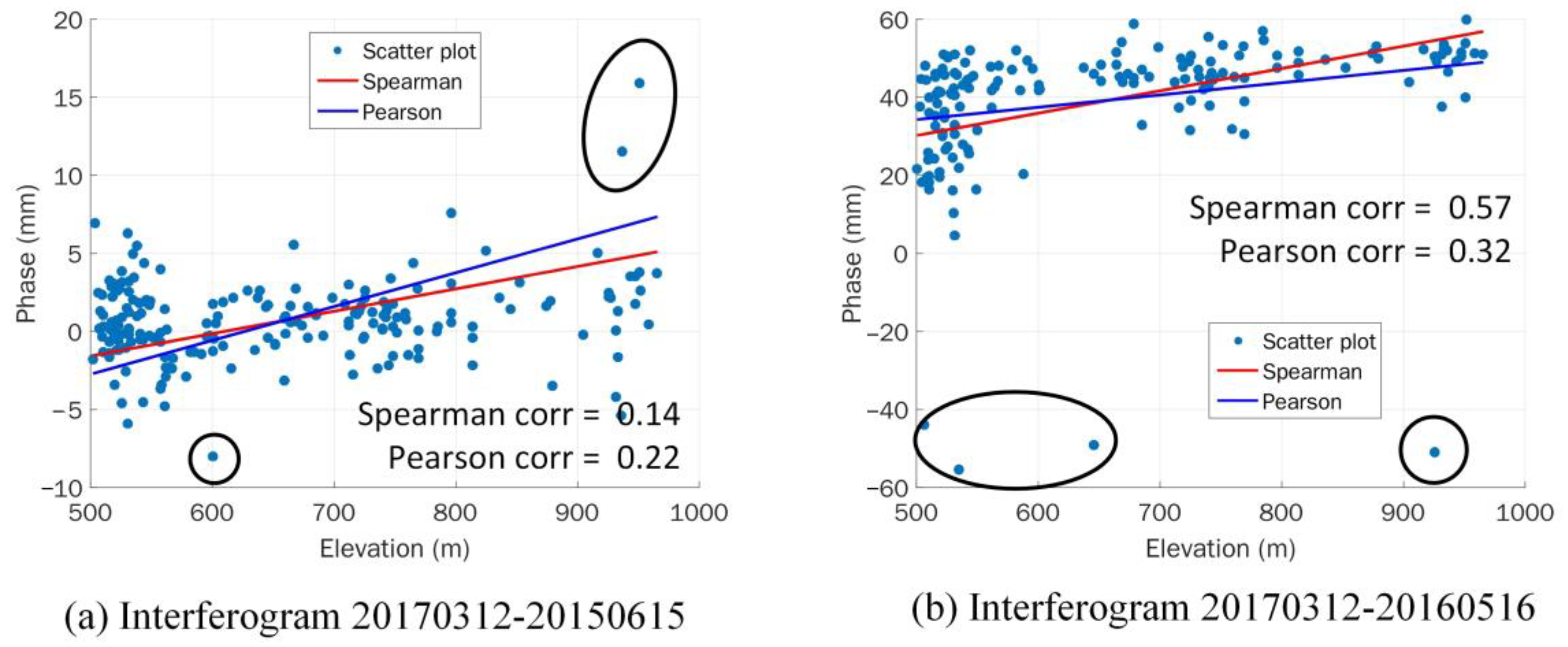
3.1.3. Spearman’s Rank Correlation between Phase and Elevation
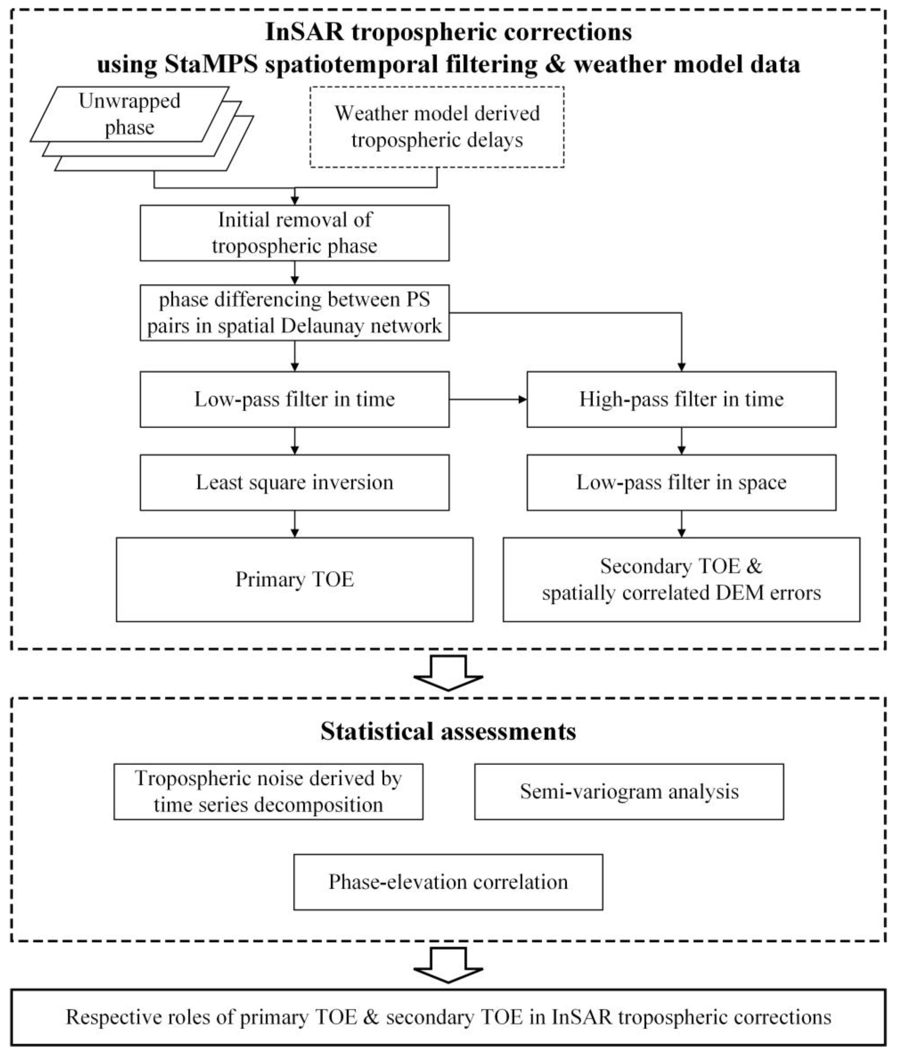
3.2. Analysis of Primary and Secondary Images’ Contribution in Tropospheric Corrections
4. Experiments and Results
4.1. Experimental Settings
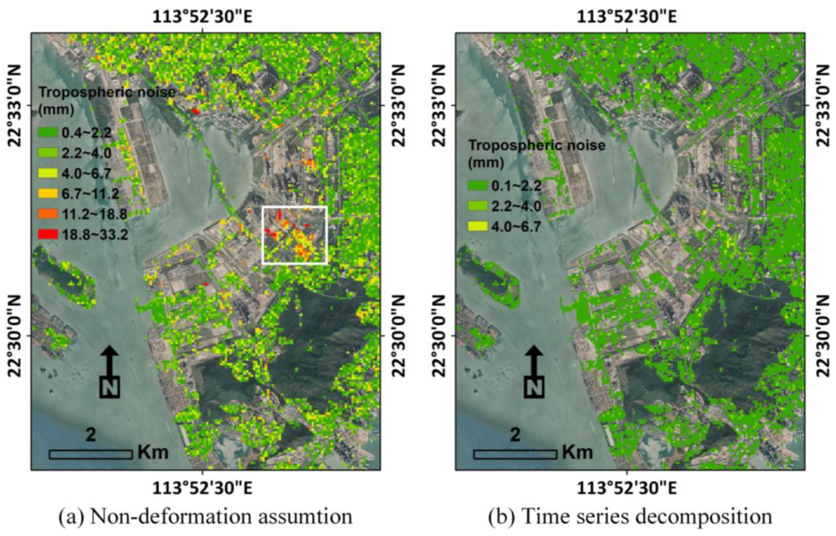
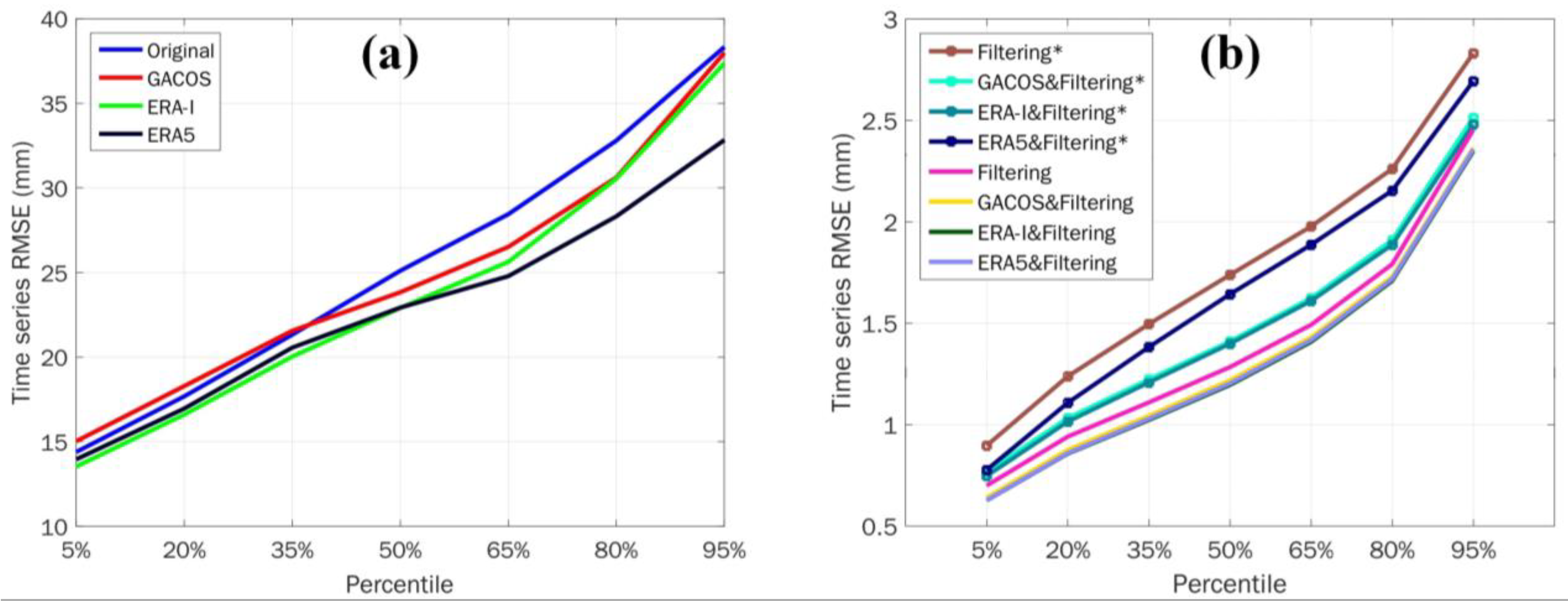
4.2. Elimination of Overall Tropospheric Noise
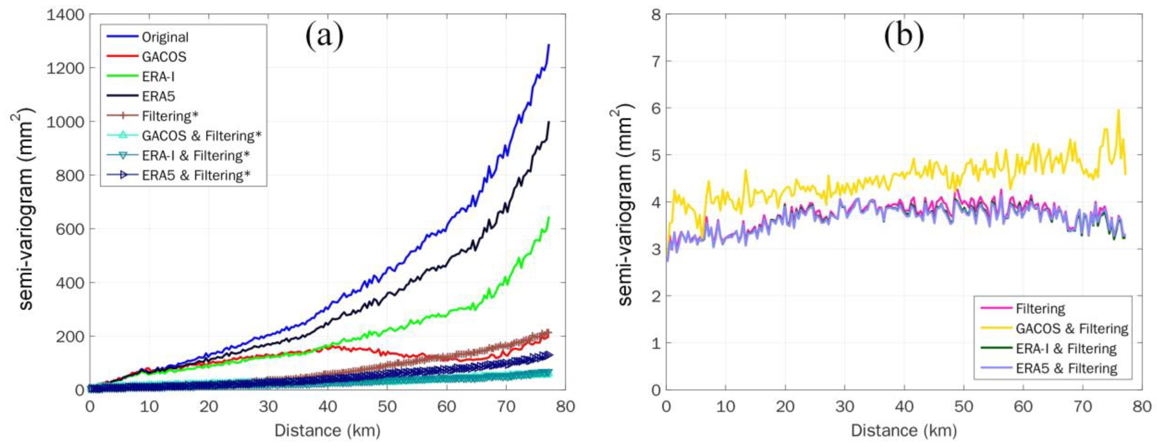
4.3. Mitigation of Distance-Dependent Signals
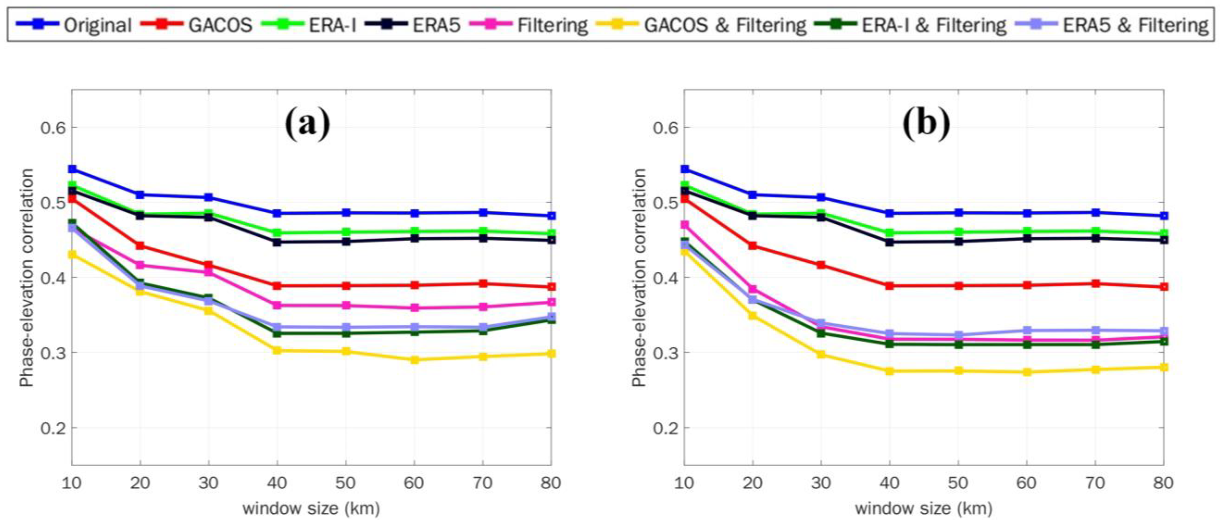
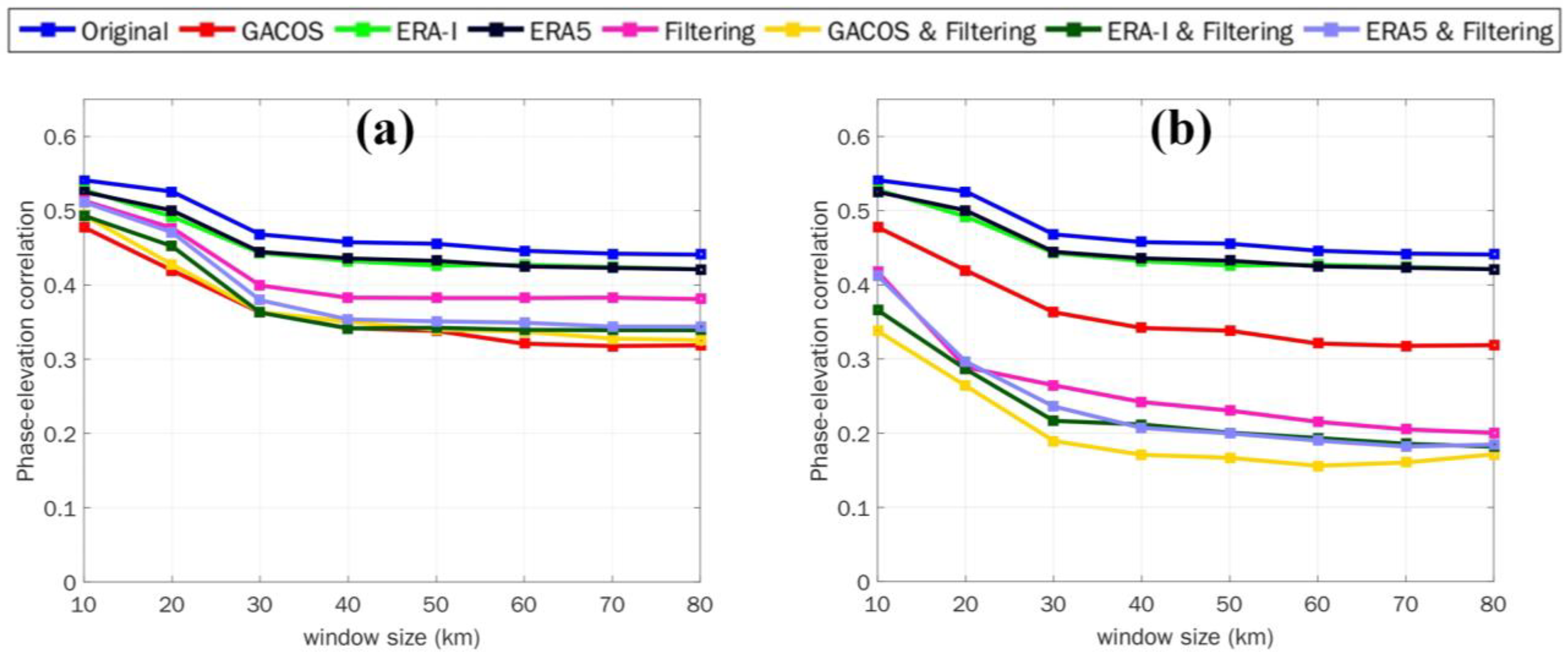
4.4. Reduction of Phase-Elevation Dependence
4.5. The Roles of Primary and Secondary TOE in Tropospheric Corrections
4.6. Local Subsidence Maps Derived after Tropospheric Correction
5. Discussion
5.1. The Applicability and Limitations of Different InSAR Tropospheric Correction Methods
5.2. Comparison of ERA-I, ERA5, and GACOS for the Tropospheric Correction in Coastal Areas
6. Conclusions
Author Contributions
Funding
Data Availability Statement
Conflicts of Interest
References
- Ferretti, A.; Prati, C.; Rocca, F. Permanent Scatterers in SAR Interferometry. IEEE Trans. Geosci. Remote Sens. 2001, 39, 8–20. [Google Scholar] [CrossRef]
- Hooper, A.; Segall, P.; Zebker, H. Persistent Scatterer Interferometric Synthetic Aperture Radar for Crustal Deformation Analysis, with Application to Volcán Alcedo, Galápagos. J. Geophys. Res. Solid Earth 2007, 112. [Google Scholar] [CrossRef] [Green Version]
- Berardino, P.; Fornaro, G.; Lanari, R.; Sansosti, E. A New Algorithm for Surface Deformation Monitoring Based on Small Baseline Differential SAR Interferograms. IEEE Trans. Geosci. Remote Sens. 2002, 40, 2375–2383. [Google Scholar] [CrossRef] [Green Version]
- Ferretti, A.; Fumagalli, A.; Novali, F.; Prati, C.; Rocca, F.; Rucci, A. A New Algorithm for Processing Interferometric Data-Stacks: SqueeSAR. IEEE Trans. Geosci. Remote Sens. 2011, 49, 3460–3470. [Google Scholar] [CrossRef]
- Haji-Aghajany, S.; Amerian, Y. Atmospheric Phase Screen Estimation for Land Subsidence Evaluation by InSAR Time Series Analysis in Kurdistan, Iran. J. Atmos. Sol.-Terr. Phys. 2020, 205, 105314. [Google Scholar] [CrossRef]
- Fournier, T.; Pritchard, M.E.; Finnegan, N. Accounting for Atmospheric Delays in InSAR Data in a Search for Long-Wavelength Deformation in South America. IEEE Trans. Geosci. Remote Sens. 2011, 49, 3856–3867. [Google Scholar] [CrossRef]
- Yip, S.T.H.; Biggs, J.; Albino, F. Reevaluating Volcanic Deformation Using Atmospheric Corrections: Implications for the Magmatic System of Agung Volcano, Indonesia. Geophys. Res. Lett. 2019, 46, 13704–13711. [Google Scholar] [CrossRef] [Green Version]
- Doin, M.-P.; Lasserre, C.; Peltzer, G.; Cavalié, O.; Doubre, C. Corrections of Stratified Tropospheric Delays in SAR Interferometry: Validation with Global Atmospheric Models. J. Appl. Geophys. 2009, 69, 35–50. [Google Scholar] [CrossRef]
- Massonnet, D.; Feigl, K.L. Discrimination of Geophysical Phenomena in Satellite Radar Interferograms. Geophys. Res. Lett. 1995, 22, 1537–1540. [Google Scholar] [CrossRef]
- Sandwell, D.T.; Price, E.J. Phase Gradient Approach to Stacking Interferograms. J. Geophys. Res. Solid Earth 1998, 103, 30183–30204. [Google Scholar] [CrossRef] [Green Version]
- Emardson, T.R.; Simons, M.; Webb, F.H. Neutral Atmospheric Delay in Interferometric Synthetic Aperture Radar Applications: Statistical Description and Mitigation. J. Geophys. Res. Solid Earth 2003, 108. [Google Scholar] [CrossRef]
- Wicks Jr, C.W.; Dzurisin, D.; Ingebritsen, S.; Thatcher, W.; Lu, Z.; Iverson, J. Magmatic Activity beneath the Quiescent Three Sisters Volcanic Center, Central Oregon Cascade Range, USA. Geophys. Res. Lett. 2002, 29, 26-1–26-4. [Google Scholar] [CrossRef] [Green Version]
- Cavalié, O.; Doin, M.-P.; Lasserre, C.; Briole, P. Ground Motion Measurement in the Lake Mead Area, Nevada, by Differential Synthetic Aperture Radar Interferometry Time Series Analysis: Probing the Lithosphere Rheological Structure. J. Geophys. Res. Solid Earth 2007, 112. [Google Scholar] [CrossRef] [Green Version]
- Bekaert, D.P.S.; Hooper, A.; Wright, T.J. A Spatially Variable Power Law Tropospheric Correction Technique for InSAR Data. J. Geophys. Res. Solid Earth 2015, 120, 1345–1356. [Google Scholar] [CrossRef]
- Liang, H.; Zhang, L.; Ding, X.; Lu, Z.; Li, X. Toward Mitigating Stratified Tropospheric Delays in Multitemporal InSAR: A Quadtree Aided Joint Model. IEEE Trans. Geosci. Remote Sens. 2019, 57, 291–303. [Google Scholar] [CrossRef]
- Balsamo, G.; Albergel, C.; Beljaars, A.; Boussetta, S.; Brun, E.; Cloke, H.; Dee, D.; Dutra, E.; Muñoz-Sabater, J.; Pappenberger, F.; et al. ERA-Interim/Land: A Global Land Surface Reanalysis Data Set. Hydrol. Earth Syst. Sci. 2015, 19, 389–407. [Google Scholar] [CrossRef] [Green Version]
- Hersbach, H.; Bell, B.; Berrisford, P.; Horányi, A.; Sabater, J.M.; Nicolas, J.; Radu, R.; Schepers, D.; Simmons, A.; Soci, C.; et al. Global Reanalysis: Goodbye ERA-Interim, Hello ERA5. ECMWF Newsl. 2019, 159, 17–24. [Google Scholar]
- Yu, C.; Li, Z.; Penna, N.T.; Crippa, P. Generic Atmospheric Correction Model for Interferometric Synthetic Aperture Radar Observations. J. Geophys. Res. Solid Earth 2018, 123, 9202–9222. [Google Scholar] [CrossRef]
- Yu, C.; Penna, N.T.; Li, Z. Generation of Real-time Mode High-resolution Water Vapor Fields from GPS Observations. J. Geophys. Res. Atmos. 2017, 122. [Google Scholar] [CrossRef]
- Yu, C.; Li, Z.; Penna, N.T. Interferometric Synthetic Aperture Radar Atmospheric Correction Using a GPS-Based Iterative Tropospheric Decomposition Model. Remote Sens. Environ. 2018, 204, 109–121. [Google Scholar] [CrossRef]
- Li, Z.; Fielding, E.J.; Cross, P.; Preusker, R. Advanced InSAR Atmospheric Correction: MERIS/MODIS Combination and Stacked Water Vapour Models. Int. J. Remote Sens. 2009, 30, 3343–3363. [Google Scholar] [CrossRef]
- Chen, Y.; Bruzzone, L.; Jiang, L.; Sun, Q. ARU-Net: Reduction of Atmospheric Phase Screen in SAR Interferometry Using Attention-Based Deep Residual U-Net. IEEE Trans. Geosci. Remote Sens. 2021, 59, 5780–5793. [Google Scholar] [CrossRef]
- Puysségur, B.; Michel, R.; Avouac, J.-P. Tropospheric Phase Delay in Interferometric Synthetic Aperture Radar Estimated from Meteorological Model and Multispectral Imagery. J. Geophys. Res. Solid Earth 2007, 112. [Google Scholar] [CrossRef] [Green Version]
- Murray, K.D.; Bekaert, D.P.; Lohman, R.B. Tropospheric Corrections for InSAR: Statistical Assessments and Applications to the Central United States and Mexico. Remote Sens. Environ. 2019, 232, 111326. [Google Scholar] [CrossRef]
- Xiao, R.; Yu, C.; Li, Z.; He, X. Statistical Assessment Metrics for InSAR Atmospheric Correction: Applications to Generic Atmospheric Correction Online Service for InSAR (GACOS) in Eastern China. Int. J. Appl. Earth Obs. Geoinf. 2021, 96, 102289. [Google Scholar] [CrossRef]
- Hanssen, R.F. Radar Interferometry: Data Interpretation and Error Analysis; Springer: New York, NY, USA, 2001; ISBN 0-7923-6945-9. [Google Scholar]
- Liu, P.; Chen, X.; Li, Z.; Zhang, Z.; Xu, J.; Feng, W.; Wang, C.; Hu, Z.; Tu, W.; Li, H. Resolving Surface Displacements in Shenzhen of China from Time Series InSAR. Remote Sens. 2018, 10, 1162. [Google Scholar] [CrossRef] [Green Version]
- Ma, P.; Wang, W.; Zhang, B.; Wang, J.; Shi, G.; Huang, G.; Chen, F.; Jiang, L.; Lin, H. Remotely Sensing Large- and Small-Scale Ground Subsidence: A Case Study of the Guangdong–Hong Kong–Macao Greater Bay Area of China. Remote Sens. Environ. 2019, 232, 111282. [Google Scholar] [CrossRef]
- Dong, J.; Zhang, L.; Liao, M.; Gong, J. Improved Correction of Seasonal Tropospheric Delay in InSAR Observations for Landslide Deformation Monitoring. Remote Sens. Environ. 2019, 233, 111370. [Google Scholar] [CrossRef]
- Kirui, P.K.; Reinosch, E.; Isya, N.; Riedel, B.; Gerke, M. Mitigation of Atmospheric Artefacts in Multi Temporal InSAR: A Review. PFG 2021, 89, 251–272. [Google Scholar] [CrossRef]
- Webster, R.; Oliver, M.A. Geostatistics for Environmental Scientists; John Wiley & Sons: Hoboken, NJ, USA, 2007; ISBN 0-470-51726-3. [Google Scholar]
- Hanssen, R.F.; Weckwerth, T.M.; Zebker, H.A.; Klees, R. High-Resolution Water Vapor Mapping from Interferometric Radar Measurements. Science 1999, 283, 1297–1299. [Google Scholar] [CrossRef] [Green Version]
- Elliott, J.R.; Biggs, J.; Parsons, B.; Wright, T.J. InSAR Slip Rate Determination on the Altyn Tagh Fault, Northern Tibet, in the Presence of Topographically Correlated Atmospheric Delays. Geophys. Res. Lett. 2008, 35. [Google Scholar] [CrossRef] [Green Version]
- Parker, A.L.; Biggs, J.; Walters, R.J.; Ebmeier, S.K.; Wright, T.J.; Teanby, N.A.; Lu, Z. Systematic Assessment of Atmospheric Uncertainties for InSAR Data at Volcanic Arcs Using Large-Scale Atmospheric Models: Application to the Cascade Volcanoes, United States. Remote Sens. Environ. 2015, 170, 102–114. [Google Scholar] [CrossRef] [Green Version]
- Mukaka, M. Statistics Corner: A Guide to Appropriate Use of Correlation in Medical Research. Malawi Med. J. 2012, 24, 69–71. [Google Scholar]
- Cohen, L.; Jarvis, P.; Fowler, J. Practical Statistics for Field Biology; John Wiley & Sons: Hoboken, NJ, USA, 2013; ISBN 1-118-68564-4. [Google Scholar]
- Ramsey, P.H. Critical Values for Spearman’s Rank Order Correlation. J. Educ. Stat. 1989, 14, 245–253. [Google Scholar]
- Tymofyeyeva, E.; Fialko, Y. Mitigation of Atmospheric Phase Delays in InSAR Data, with Application to the Eastern California Shear Zone. J. Geophys. Res. Solid Earth 2015, 120, 5952–5963. [Google Scholar] [CrossRef]
- Yagüe-Martínez, N.; Prats-Iraola, P.; González, F.R.; Brcic, R.; Shau, R.; Geudtner, D.; Eineder, M.; Bamler, R. Interferometric Processing of Sentinel-1 TOPS Data. IEEE Trans. Geosci. Remote Sens. 2016, 54, 2220–2234. [Google Scholar] [CrossRef] [Green Version]
- Hooper, A.; Zebker, H. Phase Unwrapping in Three Dimensions with Application to InSAR Time Series. J. Opt. Soc. Am. A 2007, 24, 2737–2747. [Google Scholar] [CrossRef] [Green Version]
- Bekaert, D.P.S.; Walters, R.J.; Wright, T.J.; Hooper, A.J.; Parker, D.J. Statistical Comparison of InSAR Tropospheric Correction Techniques. Remote Sens. Environ. 2015, 170, 40–47. [Google Scholar] [CrossRef] [Green Version]
- Schwanghart, W. Variogramfit. Available online: https://ww2.mathworks.cn/matlabcentral/fileexchange/25948-variogramfit (accessed on 16 February 2023).
- Christakos, G. Modern Spatiotemporal Geostatistics; Oxford University Press: Oxford, UK, 2000; Volume 6, ISBN 0-19-803179-3. [Google Scholar]
- Jolivet, R.; Agram, P.S.; Lin, N.Y.; Simons, M.; Doin, M.P.; Peltzer, G.; Li, Z. Improving InSAR Geodesy Using Global Atmospheric Models. J. Geophys. Res. Solid Earth 2014, 119, 2324–2341. [Google Scholar] [CrossRef]


| Sentinel-1 IW SLC Data | |
|---|---|
| Timespan | 15 June 2015~7 March 2018 |
| Revisit cycle (days) | 12 |
| Polarization | VV |
| Incidence angle (°) | 41.69~46.11 |
| Wavelength (cm) | 5.5 |
| Slant range spacing (m) | 2.33 |
| Azimuth spacing (m) | 13.92 |
| |rs| | Correlation Strength |
|---|---|
| 0.00~0.19 | Very weak |
| 0.20~0.39 | Weak |
| 0.40~0.69 | Moderate |
| 0.70~0.89 | Strong |
| 0.90~1.00 | Very strong |
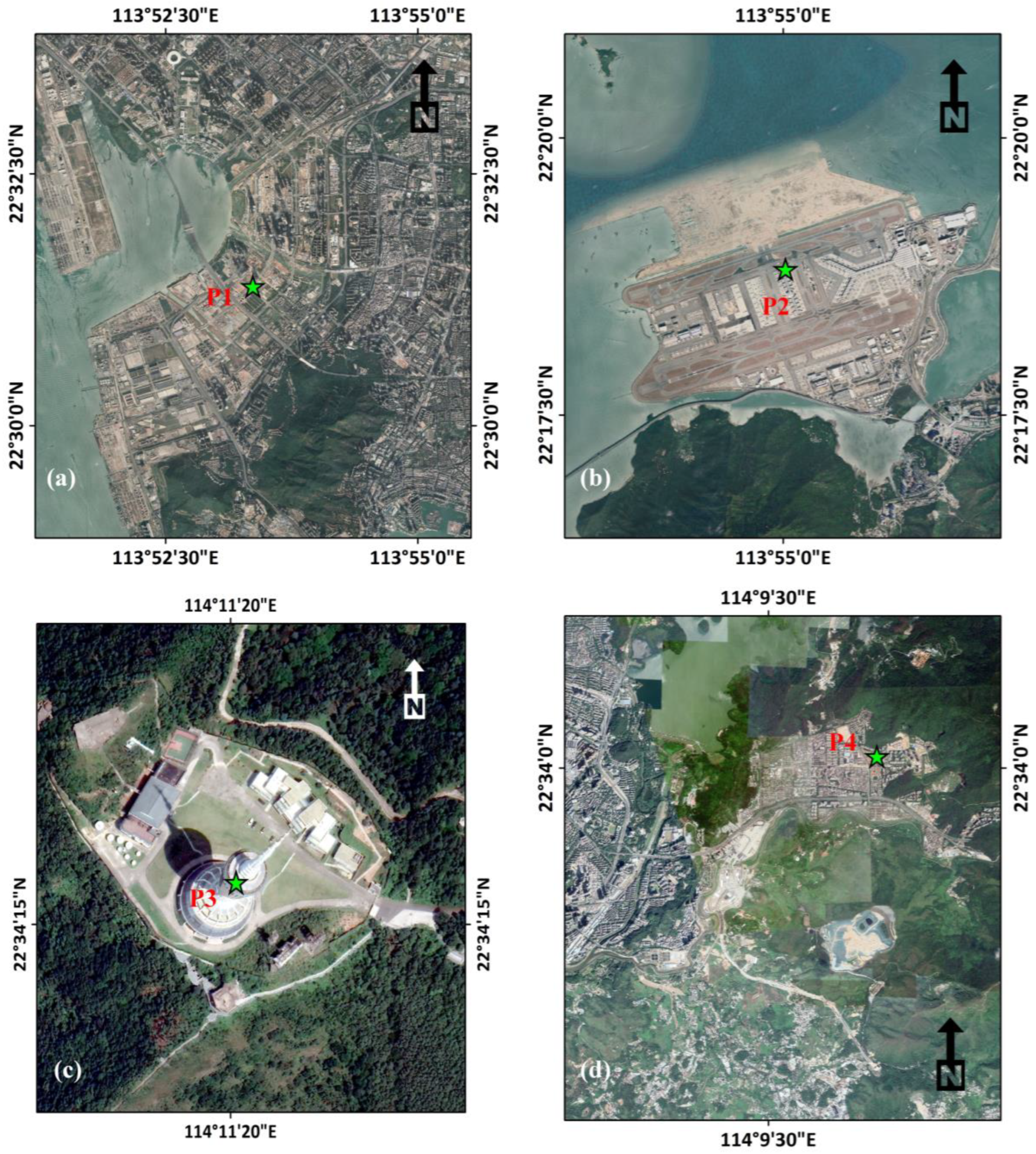
| Latitude | Longitude | Altitude | Topography | |
|---|---|---|---|---|
| P1 | N 22.523119° | E 113.889458° | −3.6 m | Low altitude, flat terrain, ocean-reclaimed area |
| P2 | N 22.313656° | E 113.917023° | −1.1 m | Low altitude, flat terrain, ocean-reclaimed area |
| P3 | N 22.571257° | E 114.188890° | 639 m | High altitude, hilly area |
| P4 | N 22.568163° | E 114.171921° | 39.4 m | Low altitude, flat terrain, metro tunneling area |
| Weighted Mean Range (km) | Weighted Mean Sill (mm) | ||
|---|---|---|---|
| Original | No correction | 53.20 | 761.39 |
| Group 1 | GACOS | 48.19 | 561.66 |
| ERA-I | 50.57 | 489.88 | |
| ERA5 | 51.50 | 563.68 | |
| Group 2 | Spatiotemporal filtering * | 63.57 | 223.61 |
| GACOS and filtering * | 76.61 | 71.92 | |
| ERA-I and filtering * | 61.41 | 63.82 | |
| ERA5 and filtering * | 63.57 | 134.54 | |
| Group 3 | Spatiotemporal filtering | 15.97 | 2.79 |
| GACOS and filtering | 16.75 | 3.34 | |
| ERA-I and filtering | 13.72 | 2.86 | |
| ERA5 and filtering | 13.78 | 3.50 |
Disclaimer/Publisher’s Note: The statements, opinions and data contained in all publications are solely those of the individual author(s) and contributor(s) and not of MDPI and/or the editor(s). MDPI and/or the editor(s) disclaim responsibility for any injury to people or property resulting from any ideas, methods, instructions or products referred to in the content. |
© 2023 by the authors. Licensee MDPI, Basel, Switzerland. This article is an open access article distributed under the terms and conditions of the Creative Commons Attribution (CC BY) license (https://creativecommons.org/licenses/by/4.0/).
Share and Cite
Sun, L.; Chen, J.; Li, H.; Guo, S.; Han, Y. Statistical Assessments of InSAR Tropospheric Corrections: Applicability and Limitations of Weather Model Products and Spatiotemporal Filtering. Remote Sens. 2023, 15, 1905. https://doi.org/10.3390/rs15071905
Sun L, Chen J, Li H, Guo S, Han Y. Statistical Assessments of InSAR Tropospheric Corrections: Applicability and Limitations of Weather Model Products and Spatiotemporal Filtering. Remote Sensing. 2023; 15(7):1905. https://doi.org/10.3390/rs15071905
Chicago/Turabian StyleSun, Luyi, Jinsong Chen, Hongzhong Li, Shanxin Guo, and Yu Han. 2023. "Statistical Assessments of InSAR Tropospheric Corrections: Applicability and Limitations of Weather Model Products and Spatiotemporal Filtering" Remote Sensing 15, no. 7: 1905. https://doi.org/10.3390/rs15071905