

A Comparison of UAV-Derived Dense Point Clouds Using LiDAR and NIR Photogrammetry in an Australian Eucalypt Forest

School of Biology and Environmental Science, Queensland University of Technology, 2 George Street, Brisbane, QLD 4000, Australia
*
Author to whom correspondence should be addressed.
Remote Sens. 2023, 15(6), 1694; https://doi.org/10.3390/rs15061694
Submission received: 24 February 2023
/
Revised: 5 March 2023
/
Accepted: 16 March 2023
/
Published: 21 March 2023
(This article belongs to the Special Issue Drones, Artificial Intelligence and Advanced Analytics for the Conservation of Threatened Species)
Abstract
:Light detection and ranging (LiDAR) has been a tool of choice for 3D dense point cloud reconstructions of forest canopy over the past two decades, but advances in computer vision techniques, such as structure from motion (SfM) photogrammetry, have transformed 2D digital aerial imagery into a powerful, inexpensive and highly available alternative. Canopy modelling is complex and affected by a wide range of inputs. While studies have found dense point cloud reconstructions to be accurate, there is no standard approach to comparing outputs or assessing accuracy. Modelling is particularly challenging in native eucalypt forests, where the canopy displays abrupt vertical changes and highly varied relief. This study first investigated whether a remotely sensed LiDAR dense point cloud reconstruction of a native eucalypt forest completely reproduced canopy cover and accurately predicted tree heights. A further comparison was made with a photogrammetric reconstruction based solely on near-infrared (NIR) imagery to gain some insight into the contribution of the NIR spectral band to the 3D SfM reconstruction of native dry eucalypt open forest. The reconstructions did not produce comparable canopy height models and neither reconstruction completely reproduced canopy cover nor accurately predicted tree heights. Nonetheless, the LiDAR product was more representative of the eucalypt canopy than SfM-NIR. The SfM-NIR results were strongly affected by an absence of data in many locations, which was related to low canopy penetration by the passive optical sensor and sub-optimal feature matching in the photogrammetric pre-processing pipeline. To further investigate the contribution of NIR, future studies could combine NIR imagery captured at multiple solar elevations. A variety of photogrammetric pre-processing settings should continue to be explored in an effort to optimise image feature matching.
Keywords:
canopy; drone; eucalyptus; forest structure; lidar; NIR; photogrammetry; remote sensing; UAV1. Introduction
Information about forest structure is essential for those tasked with managing forests and their ecosystem functions [1]. Forest structure describes the spatial arrangement of a forest’s components, including the abundance and distribution of vegetation elements, both vertically and horizontally [2]. Accurate mapping and quantification of components such as the canopy and shrub cover are essential to environmental monitoring, with applications as varied as hydrological modelling, fire and biodiversity management and carbon storage [3,4]. Gathering sufficient data in the field can be impractical [5] as ground surveys can be limited, both spatially and temporally, by access and resource constraints [6]. As a result, structural analyses increasingly utilise small, unmanned aerial vehicles (UAVs) [1]. UAVs allow data to be remotely gathered from otherwise inaccessible areas [7]. They are also cheaper and more available than satellite and manned airborne platforms [2] and offer enhanced operational flexibility [8]. Continual development in remote sensing technologies, in combination with the uptake of UAVs, has revolutionised the collection of high-resolution data and transformed our ability to map and assess forest attributes [2,9], although results vary among the different platforms and methods [10].
Remote sensing may be passive or active. Passive sensors detect reflected solar radiation [11] and include digital multispectral and hyperspectral cameras [8] that generate two-dimensional (2D) images within narrow, discrete spectral bands [12]. Active sensors emit their own light [11]. The most commonly used active sensors are light detection and ranging (LiDAR) systems [6]. LiDAR systems emit laser pulses which are reflected back from an object or surface and detected upon return [13]. Range measurements are calculated with the LiDAR sensor based on the time-in-flight between emission and return of the pulse [2]. These measurements locate scanned objects in three-dimensional (3D) space [11] and generate 3D point clouds that are spatially accurate representations of the objects’ shapes [9].
For the past two decades, LiDAR has been the tool of choice for mapping vertical canopy structures and estimating the structural attributes of forests [9,14,15]. Low-altitude flight capability allows UAV-LiDAR to produce ultra-high-density point clouds [16]. However, recent advances in computer vision techniques, such as structure from motion (SfM) photogrammetry, have transformed 2D digital aerial imagery into a powerful, inexpensive and highly available alternative [2]. The use of SfM to simultaneously estimate 3D scene geometry, camera pose and calibration parameters [17], in combination with multiview stereo image matching, has made it relatively simple to generate LiDAR-like multispectral point clouds from 2D imagery [5], which can be used to predict forest attributes such as tree height and horizontal canopy structure [18]. UAV-derived imagery captures structural and spectral data at high spatial and temporal resolutions [5] that is well-suited to local-scale ecosystem modelling [19]. However, remotely sensed imagery is less effective at predicting vertical forest structure, particularly as crown closure increases [20], as only the uppermost surface is captured [14]. Digital aerial imagery is also negatively affected by shadows, particularly in mature forests where the canopy is dense and multi-layered [9]. The amount of shadow tends to increase when UAV imagery is captured in low solar angle conditions on sunny days. While this effect can be minimised by surveying on cloudy days, the lower light levels tend to reduce contrast and increase alignment error [5]. Shadows are particularly problematic when orthomosaics are derived from UAV imagery [21]. Radiometric or spectral calibration is sometimes required to compensate for fluctuations in weather and illumination conditions during data capture, but this is more likely to be undertaken when spectral or vegetation indices are to be calculated [22]. Camera settings such as shutter speed and focal length can also be adjusted during UAV image collection in response to changing light conditions [23].
Canopy modelling is particularly complex in native eucalypt forests where the crown structure is clumped on two levels, leaves are vertically oriented and leaves and canopy clumps are easily moved by the wind [24,25]. Canopy cover in these forests generally ranges from 50 to 80%, resulting in a sunlit environment that produces a floor of fire-tolerant, hard-leaved shrubs and grasses in dry environments and tree ferns and small rainforest shrubs in the wet [26]. The canopy structure and density are distinctly different to that of coniferous and boreal forests, in which most research has been conducted to date [27], which represents a more difficult target for 3D SfM reconstruction [24].
There are numerous examples in the literature where airborne LiDAR has been used to model eucalypts grown in plantations [9,28,29,30,31,32,33]. However, plantations tend towards regular tree spacings and therefore differ substantially in structure from native forests. By comparison, relatively few LiDAR studies have been undertaken in native eucalypt forests [34], although recent bushfires in eastern Australia appear to be driving an increase in modelling that is focussed on fuel metrics and post-bushfire resilience ([23] (also uses SfM)) and [34,35,36].
Among the few examples of native eucalypt LiDAR studies, several have been conducted in wet eucalypt forests [23,35,37,38,39], which have a different species composition to dry eucalypt forests and therefore different structural attributes. Wet eucalypt species tend to attain much greater heights, for example, mountain ash (Eucalyptus regnans) can grow to 80 m, while alpine ash (E. delegatensis) and shining gum (E. nitens) can grow to 60 m [40]. Combined with different understoreys, the wet and dry native eucalypt forests represent unique and distinct modelling challenges. Examples in which native dry eucalypt forest has been modelled with airborne LiDAR data include a comparison of LiDAR models with SfM dense point clouds and field-measured metrics [2] and an examination of projective cover models in the context of native Australian eucalypt vegetation [41].
Studies involving photogrammetric SfM reconstructions of eucalypt forests are also often based on plantation stands or forest farms [9,42,43,44,45]. A 2020 photogrammetric study in an Australian native dry eucalypt open forest focussed on tree diameters rather than canopy characteristics [46]. One study that did focus on photogrammetric canopy metrics investigated the effect of variables such as flight parameters, sensors and system settings on native dry eucalypt canopy reconstructions [24]. The latter study suggested that the NIR spectral band (770–810 nm) had a positive effect on the completeness of the reconstructions.
This study aims to add to the relatively sparse literature on UAV-derived canopy models in native dry eucalypt open forests and has three objectives. First, to assess the effectiveness of UAV-LiDAR for canopy modelling in a native dry eucalypt open forest by constructing a UAV-LiDAR-derived canopy height model (CHM) and comparing the CHM tree heights and density values against field measurements. Second, to construct a UAV-SfM CHM of the same native dry eucalypt open forest based solely on NIR imagery to gain some insight into the contribution of the NIR spectral band to 3D SfM reconstruction of native dry eucalypt open forest by making the same comparisons against height and density field measurements. Third, using the field measurements as a baseline, to compare the completeness and accuracy of the UAV-LiDAR CHM with the UAV-SfM-NIR CHM.
2. Materials and Methods
2.1. The Study Site
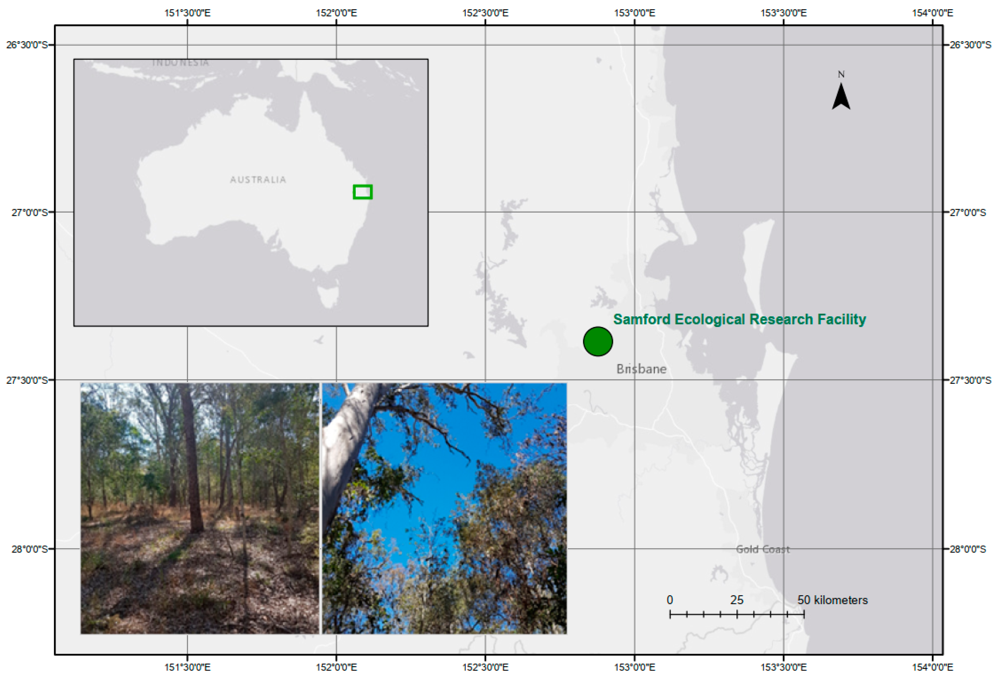
Remote and field data were collected from the Samford Ecological Research Facility (SERF) on 18 and 25 August 2020. SERF is located in the peri-urban Samford Valley approximately 24 km northwest of Brisbane at 27.37985°S and 152.87694°E (Figure 1). The vegetation at SERF is eucalypt (dry sclerophyll) open forest to woodland, predominantly Eucalyptus melanophloia and E. crebra [47].
2.2. Data
2.2.1. Remote Data
In this study, flight planning sought to optimise the data collected with each sensor. Flight planning should incorporate best practices as each platform–sensor combination requires unique adjustments to ensure the data are best suited for post-capture processing [48]. Flight parameters should deliver data that fulfil all requirements in terms of resolution, lighting and coverage [22].
LiDAR data and digital imagery were collected on separate days in bright sunshine under clear sky conditions. Sensors were carried by a DJI Matrice 600 (M600) Pro UAV platform, with an onboard flight control system equipped with a global navigation satellite system (GNSS) and inertial measurement units. Flights lasted approximately 26 min from take-off to landing.
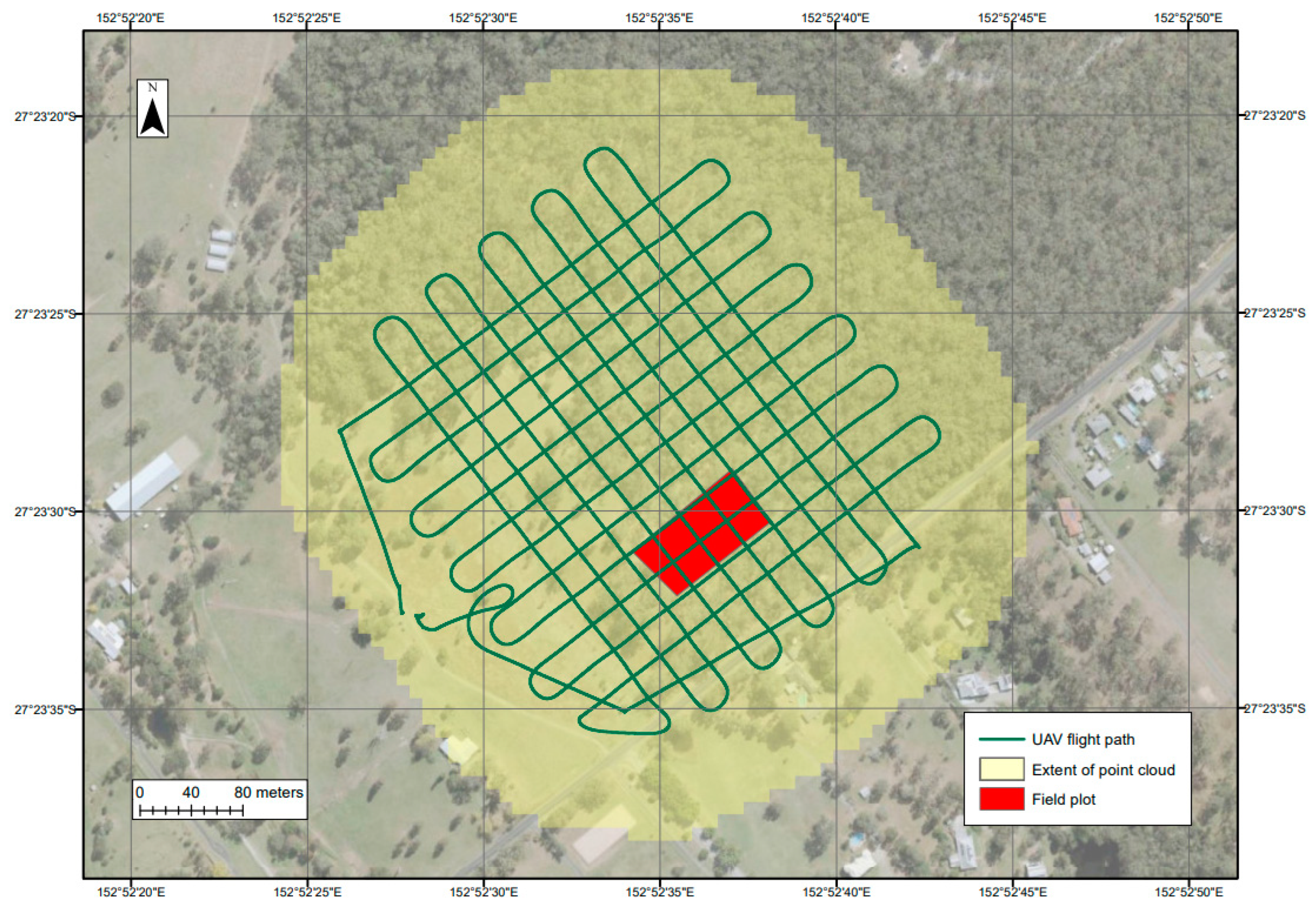
LiDAR data were collected on 18 August 2020 at ~39° solar azimuth and 41° solar elevation using an Emesent Hovermap 3D LiDAR mapping and autonomy payload, with a Velodyne Puck sensor with 360° × 360° rotating field of view (FOV). The pre-programmed flight path comprised a perpendicular grid with 30 m spacing (Figure 2) as a 90° rotation of flight lines has been found to achieve greater canopy penetration [49]. Cross-angled LiDAR capture can also reduce occlusion and achieve greater connectivity across the survey area [50]. The Hovermap flew at approximately 55 metres above ground level (mAGL) and covered approximately 8.5 ha (85,397 m2). The sensor recorded a maximum of two returns per pulse, and the survey generated 112,090,335 points.
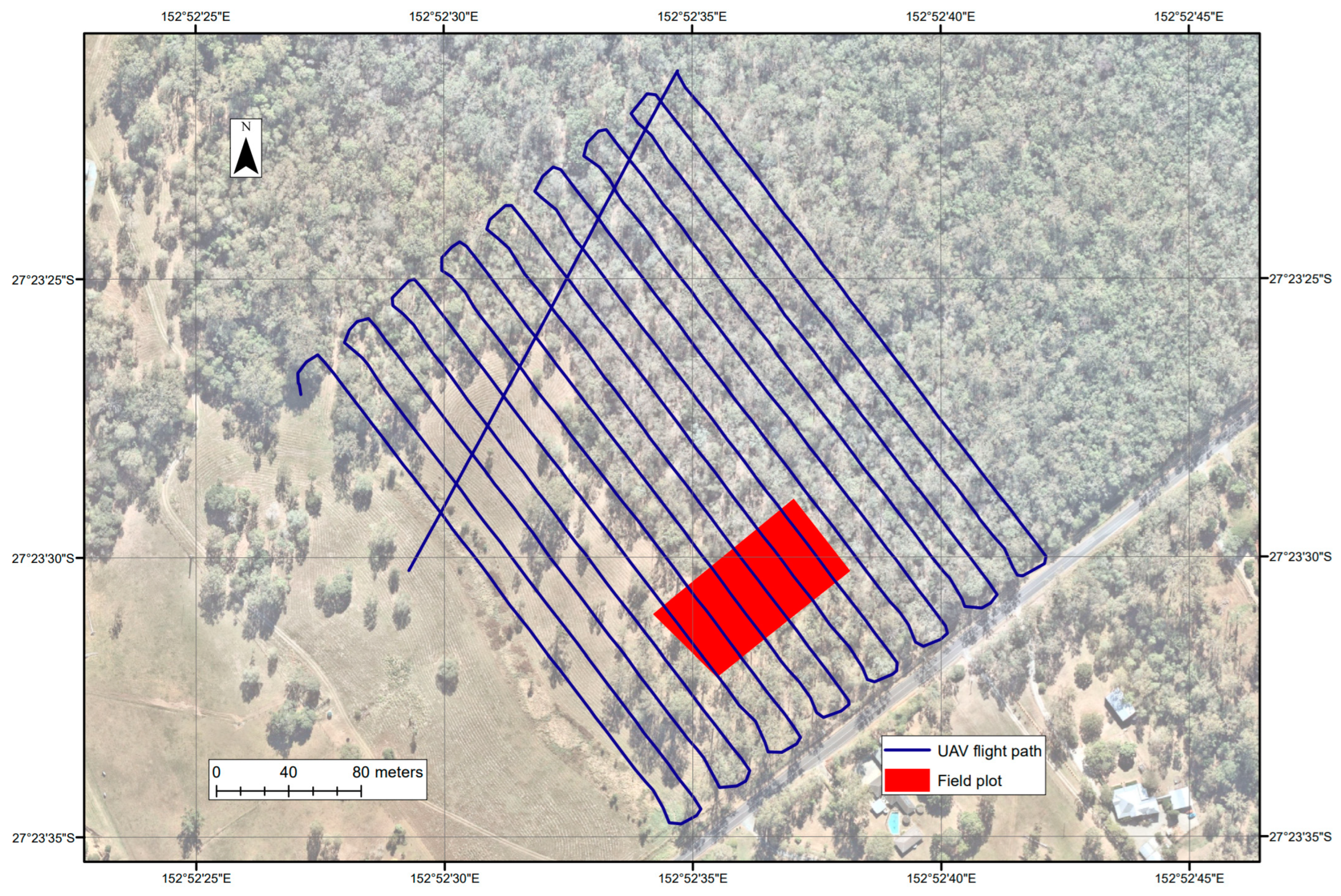
Digital NIR imagery was captured on 25 August 2020 at ~54° solar azimuth and 33° solar elevation with a MicaSense Altum multispectral and radiometric thermal sensor, with 2064 × 1544 sensor resolution and 48° horizontal × 37° vertical FOV. Images were captured every two seconds with a nadir sensor. The flight path was designed to deliver high overlap to avoid difficulties with image matching in the SfM pipeline [22]. It comprised 16 adjacent survey lines with 19 m spacing and covered the same footprint as the Hovermap (Figure 3). The target altitude of 120 mAGL resulted in a footprint of approximately 107 m perpendicular to and 80 m along flight lines at ground level, with ~89% forward lap (71 m), ~84% side lap (90 m) and an average ground sampling distance (GSD) of 5.2 cm.
2.2.2. Field Data
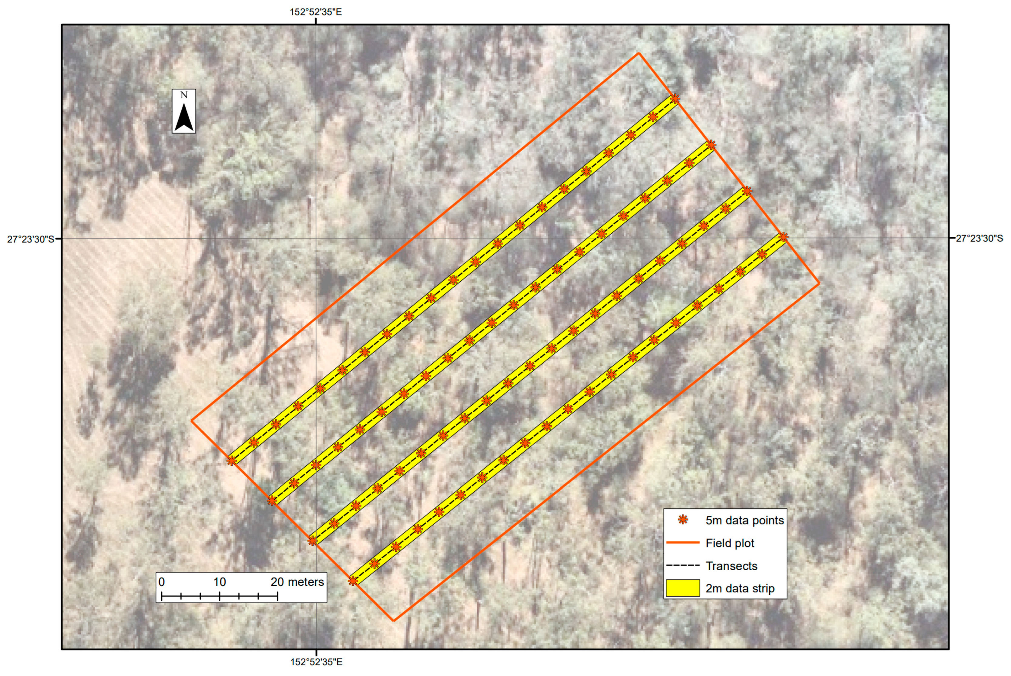
Field data were collected from a plot approximately 100 m × 50 m (actual area 4863 m2) within the UAV survey area. Four parallel 100 m transects were set out lengthwise within the plot at 10 m spacing (Figure 4). A Trimble R10 high-precision GNSS was used to georeference the plot corners. Corner coordinates were used to create shapefiles in ArcGIS v10.8 to enable field data to be compared with UAV-derived products. Additional ground control points were not required for this study.
The height of all trees with diameter-at-breast-height (DBH) >0.2 m was estimated with a range finder, and the measured trees were georeferenced with a Trimble R10. Canopy cover was estimated at 5 m intervals along each transect with the CanopyCapture mobile app v1.0.2 [51]. To avoid ambiguity, field-measured canopy cover is interpreted as “crown projective cover (CPC)” which estimates the vertical tree crown projection per unit area of the ground surface, with overlaps counted only once [41]. CPC, therefore, does not distinguish between foliage and woody elements.
2.3. Photogrammetric Pre-Processing of Digital Imagery
Ascent and descent images were trimmed, resulting in a set of 699 NIR images. Open Drone Map (WebODM Manager) v1.8.7 was used for pre-processing following a standard photogrammetric pipeline [24,52]. Default pre-processing settings (Supplementary Material, Table S1) were retained, which included the use of the Scale Invariant Feature Transform (SIFT) algorithm for feature detection and pre-matching of features across 8 images. SfM sparse point clouds were reconstructed using image feature identification and keypoint matching, while camera geometry was described using aerial triangulation. Iterative bundle adjustments were applied to image blocks to address distortion and minimise reprojection error. Multiview stereo pixel matching algorithms were used to reconstruct a 3D DPC.
2.4. DPC Processing
LiDAR and SfM-NIR DPCs were processed using CloudCompare v2.11.1–2.11.3 in the EPSG:28356 coordinate system. The LiDAR cloud was trimmed and then cleaned of noise using the statistical outlier removal (SOR) tool based on 6 points and 1 standard deviation. A field plot shapefile, with a buffer added, was used to segment the general plot area from the trimmed cloud. The segment was rasterised based on a 0.5 m grid and minimum heights were extracted to create a digital terrain model (DTM). The DTM was cleaned of noise, much of which represented lantana (Lantana camara), which is an invasive shrub that occurs in eucalypt and other native vegetation along Queensland’s coast and hinterland. Setting the DTM as the reference, points above 2 m were exported from the minimum height grid. The cloud was normalised for terrain so that all points represented height above ground level and clipped again to field plot boundaries, thus creating the final LiDAR-based CHM. The SfM-NIR DPC was then imported into Cloud Compare and segmented with the buffered field plot shapefile before being manually aligned with the LiDAR CHM (x + 3, y + 0, z − 3) and clipped to field plot boundaries.
2.5. Canopy Structure and Analysis
Maps and data visualisations were drawn in ArcGIS v10.8. Assessment and statistical analyses were based on the methods of Ref. [2]. Reconstruction of canopy cover in SFM-NIR and LiDAR CHMs was initially assessed with visual comparison and comparison with an aerial photograph of vegetation within the field plot. Statistical analyses were conducted at the field plot level using 0.2 m grid cells. Field-measured CPC was compared with the mean point density within a one-metre radius of each field data point (n = 84), for both SfM-NIR and LiDAR CHMs. Point density values were extracted from a buffered field plot to avoid edge effects. Field-measured heights of all trees within the field plot with DBH > 0.2 m (n = 45) were compared with the estimated height (absolute Z distance) at the same location in each CHM. Linear regression was performed using R Studio v3.6.3 to investigate relationships between datasets for CPC/point density and height variables, and percentiles were calculated to assess the data distribution. As per Ref. [2], root mean square error (RMSE) and bias were calculated for CHM heights as:
where n = number of observations, xir = CHM height and xif = field-measured height. Differentiation of canopy layers was based on Ref. [53], with understorey defined as <5 m, mid-canopy 5–15 m and upper canopy >15 m. The complete workflow is conceptualised in Figure 5.
3. Results
3.1. Comparison of DPC Properties
The number of points in the DPC reconstructions was reduced with each iteration (Table 1).
Similar proportions were removed in each DPC iteration, with the proportion slightly lower for SfM-NIR when trimming points below 2 mAGL from the buffered field plot (~31% SfM-NIR vs. ~33% LiDAR), but slightly higher for SfM-NIR when removing the buffer (~42% SfM-NIR vs. ~40% LiDAR). The point density of the final CHM was significantly greater for LiDAR (609 points per m2) than for SfM-NIR (96 points per m2).
3.2. Comparison of CHM Point Densities
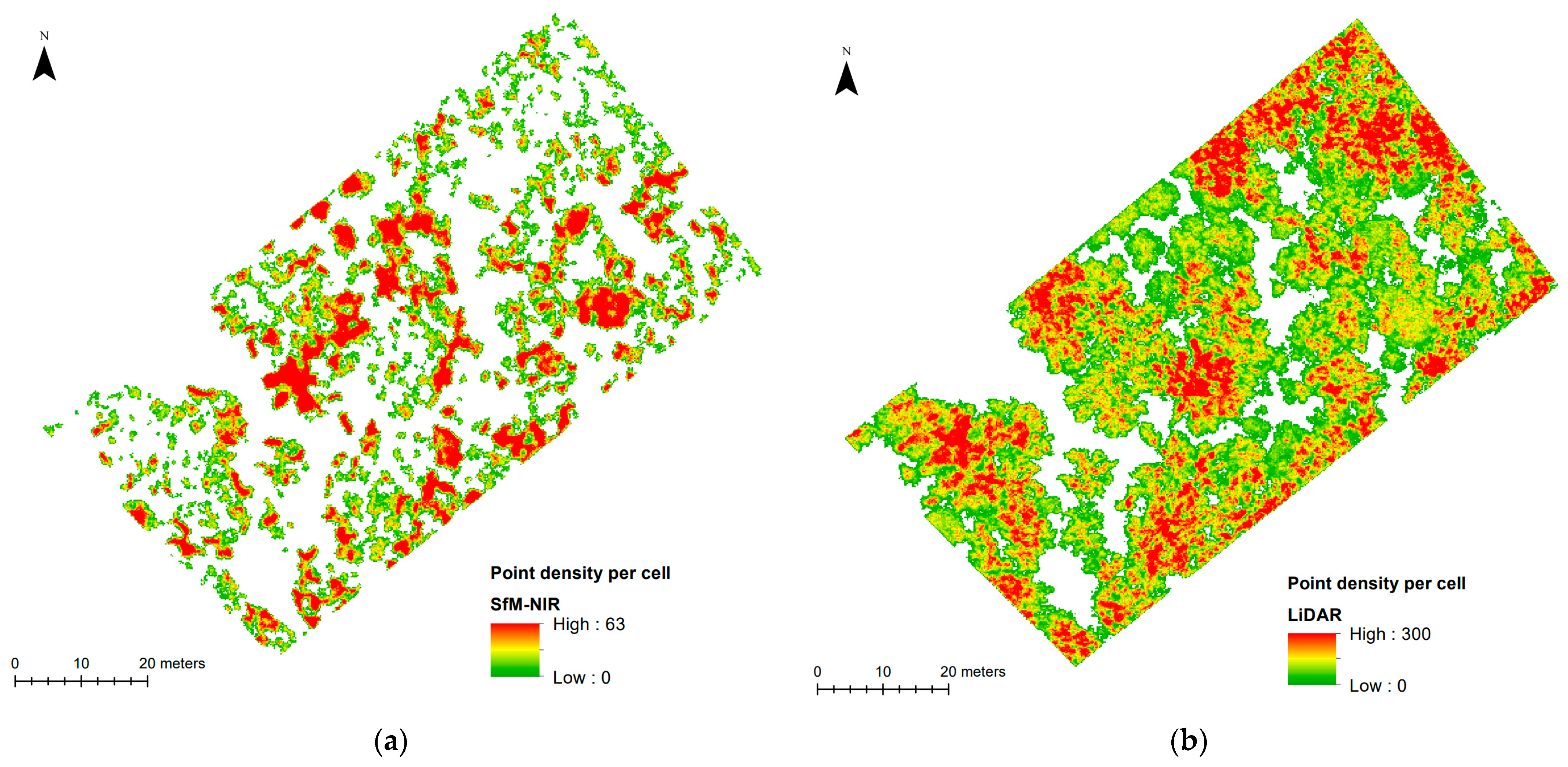
Point density ranged from 0 to 63 points per 0.2 m grid cell (mean = 1.76+/−5.64 (1 SD)) across the SfM-NIR CHM (Figure 6a) and from 0 to 300 points per 0.2 m grid cell (mean = 11.03+/−20.60 (1 SD)) across the LiDAR CHM (Figure 6b). The SfM-NIR CHM appeared to comprise mostly high and low point densities, with few mid-range values, whereas mid-range values were extensive in the LiDAR CHM (noting the large difference in density ranges between the two CHMs). Overlaying the CHMs (Figure 6c) showed that areas of high SfM-NIR point density mostly coincided with mid-range LiDAR point density. Many high-density LiDAR cells coincided with empty SfM-NIR cells (white areas), particularly in the north and southwest corners of the field plot. Low-density LiDAR cells also coincided with empty SfM-NIR cells. Low-density SfM-NIR cells mostly coincided with mid-range LiDAR cells.
The vertical point distribution profiles (Figure 7) showed that both LiDAR and SfM-NIR capture increased moving down through the upper canopy, with LiDAR capture increasing more rapidly. Both SfM-NIR and LiDAR capture decreased at ~23 m and remained relatively constant down to ~18 m, with a small spike in SfM-NIR capture at ~20 m. SfM-NIR capture increased rapidly and outstripped LiDAR capture in the mid-canopy (5–15 m). Around 12% of all SfM-NIR points were captured at ~12 m. Capture decreased for both LiDAR and SfM-NIR below 10 m. The decrease was more rapid for SfM-NIR.
3.3. Comparison of CHM Heights
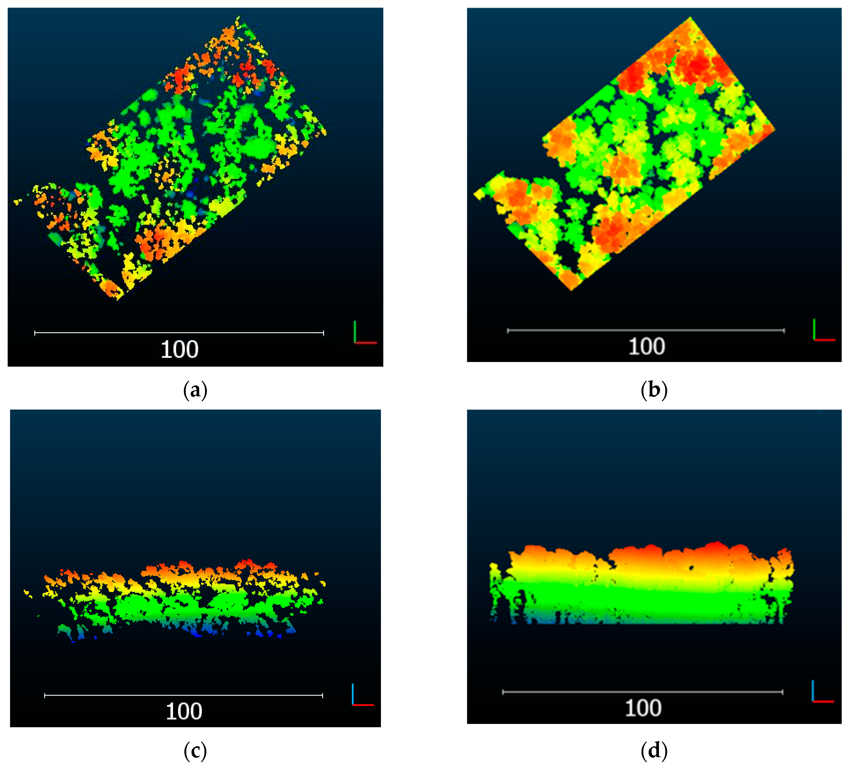
SfM-NIR CHM height ranged from 2.00 to 30.86 mAGL (mean 16.15+/−5.39 (1 SD) mAGL). LiDAR CHM height ranged from 2.00 to 31.26 mAGL (mean = 18.46+/−6.41 (1 SD) mAGL). The mean distance between the CHMs was 1.07+/−0.71 (1 SD) mAGL (RMSE = 0.3211 m). The visual comparison in CloudCompare showed that the LiDAR CHM appeared smoother and more connected than the SfM-NIR CHM (Figure 8a,b). Null values occurred in similar locations, but gaps appeared larger in the SfM-NIR CHM, particularly the gap running north–south in the eastern half of the field plot. CloudCompare elevation views (Figure 8c,d) showed the SfM-NIR CHM contained fewer data beneath the canopy, with very few tree trunks represented.
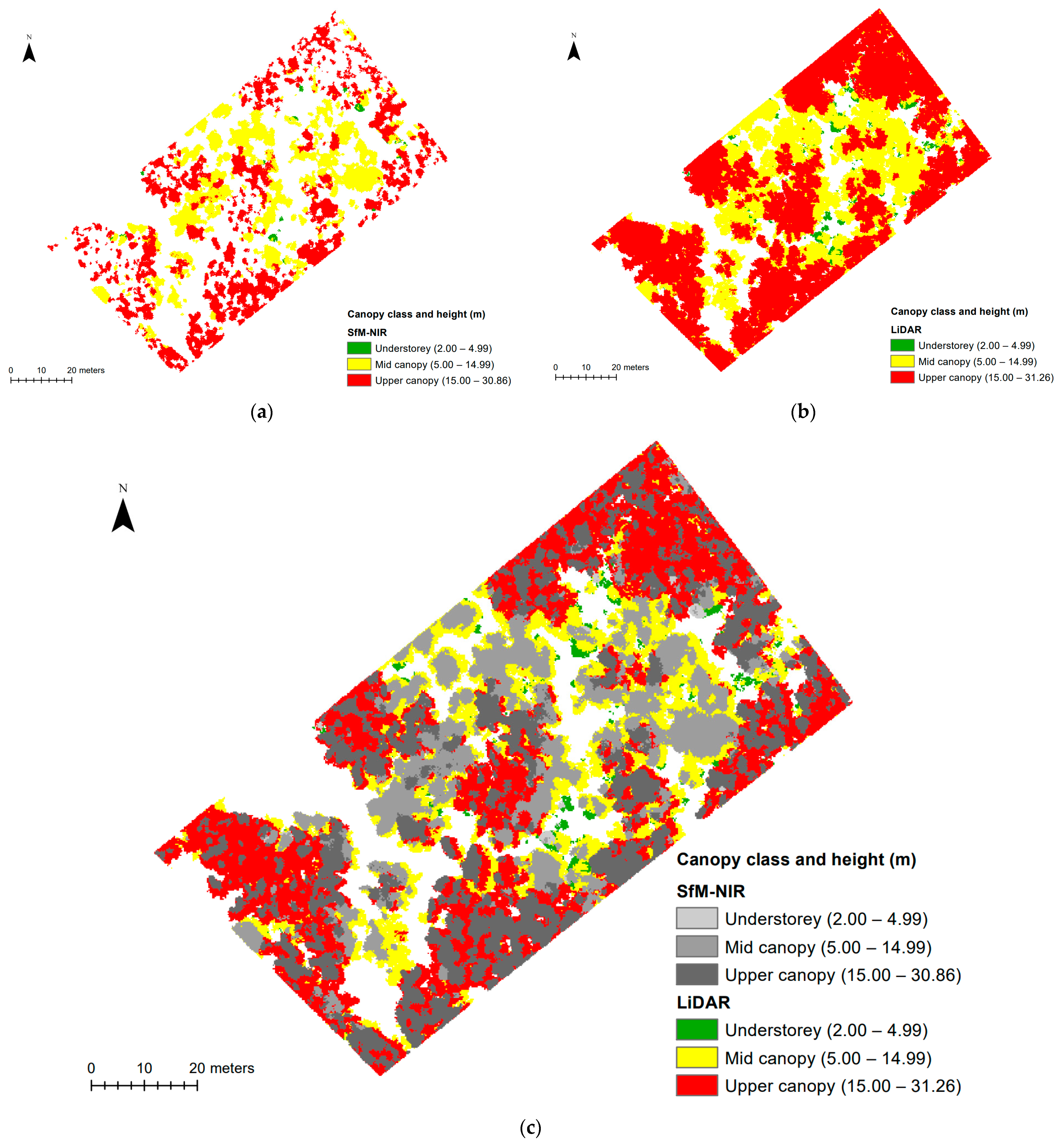
Proportional height capture with SfM-NIR (Figure 9a) equated to 0.89% understorey, 54.28% mid-canopy and 44.83% upper canopy. The upper canopy comprised the majority of LiDAR capture (63.9%), with 33.7% mid-canopy and 2.4% understorey (Figure 9b). Proportional capture was only 7.8% for SfM-NIR at 10 m, compared to 12.5% for LiDAR. In comparison with LiDAR, SFM-NiR appeared to capture only the centres of upper canopy clumps, but coincident mid-canopy areas were represented more fully (Figure 9c). Visual comparison with an aerial image showed that null values in both CHMs were generally coincident with bare ground visible through gaps in the canopy. SfM-NIR produced less cover overall, covering 72.9% of the field plot compared to 90.6% for LiDAR (Appendix A).
3.4. Comparison with Field Data—Canopy
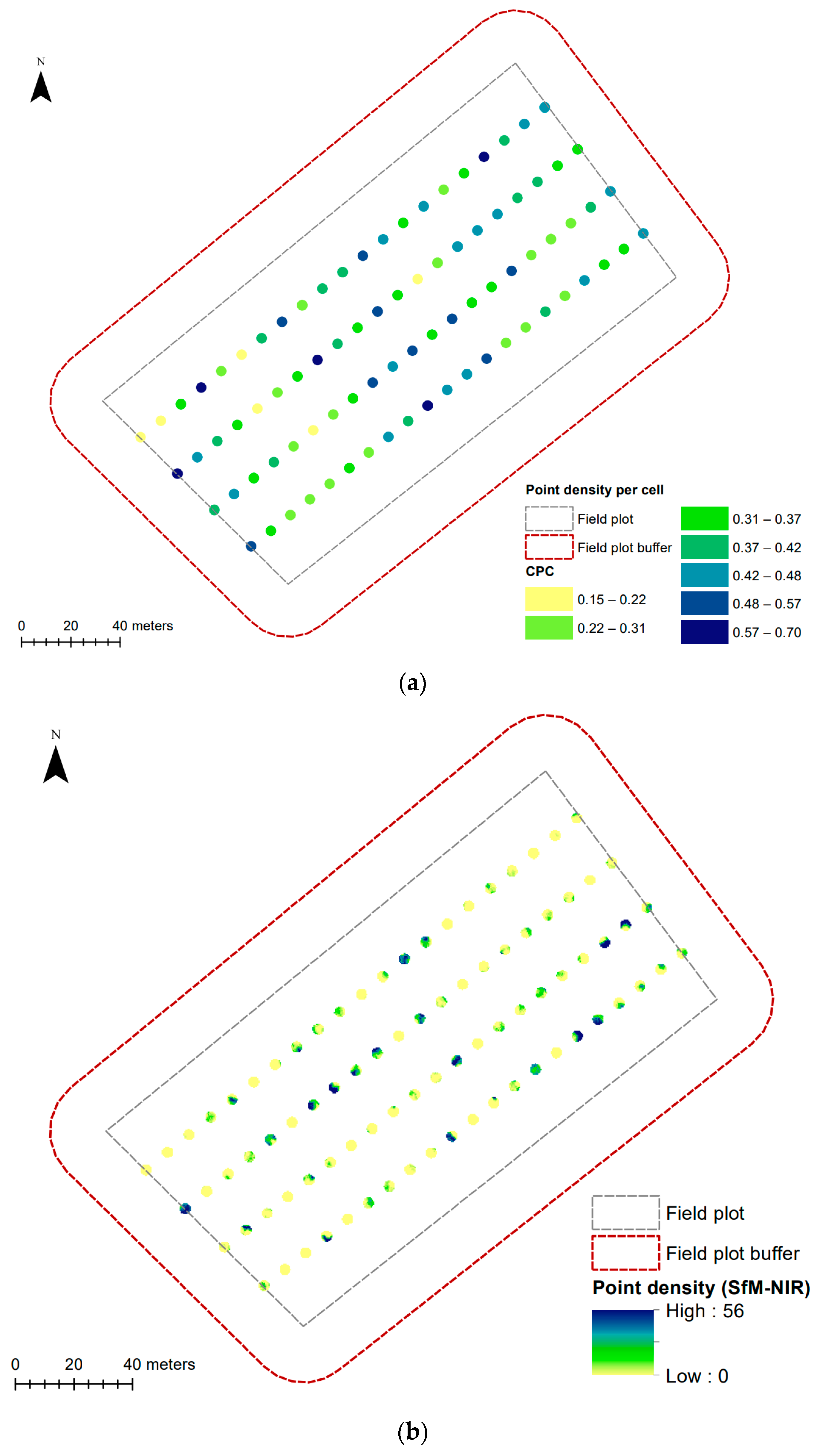
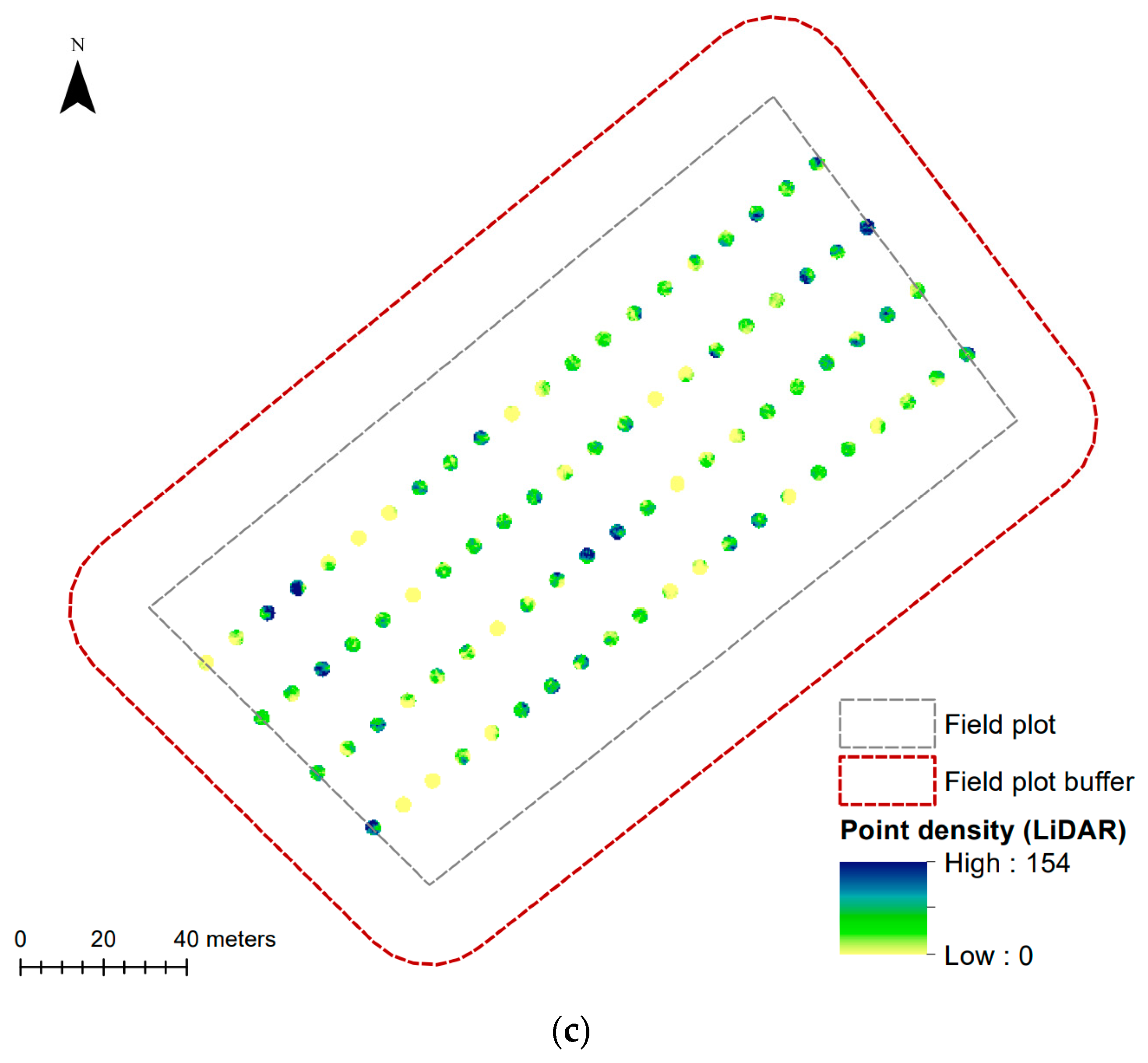
Field-measured CPC ranged from 0.15 to 0.70 (n = 84) (Figure 10a). More than 76% of locations had CPC between 0.22 and 0.48. Only 7.1% of locations had a CPC of less than 0.22 and 16.6% exceeded 0.48 (Appendix B). Point density values of individual 0.2 m grid cells within a 1 m radius of each field data point ranged from 0 to 56 points per cell in the SfM-NIR extract (Figure 10b) and from 0 to 154 for LiDAR (Figure 10c).
Point densities within each 1 m radius were aggregated, and the percentiles were calculated. The mean point density of extracted 1 m circles (3.14 m2 area) ranged from 0 to 25.41 points per 0.2 m grid cell (mean = 4.74+/−6.61 (1 SD)) in the SfM-NIR extract and from 0 to 78.92 points per 0.2 m grid cell (mean = 23.37+/−18.13 (1 SD)) for LiDAR.
The percentile values (Appendix C) were calculated to compare the spread in the extracted CHM point densities (n = 84). The interquartile range for extracted SfM-NIR values (Q1 = 0.18, Q3 = 5.90 from a maximum of 25.41) reflected the lack of mid-range point densities observed in the SfM-NIR whole-of-field-plot CHM, whereas the interquartile range for extracted LiDAR values, although still left of centre, was closer to the centre of the spread (Q1 = 7.75, Q3 = 33.04 from maximum of 78.92). The full dataset is available in Supplementary Material Table S2.
3.5. Comparison with Field Data—Tree Height
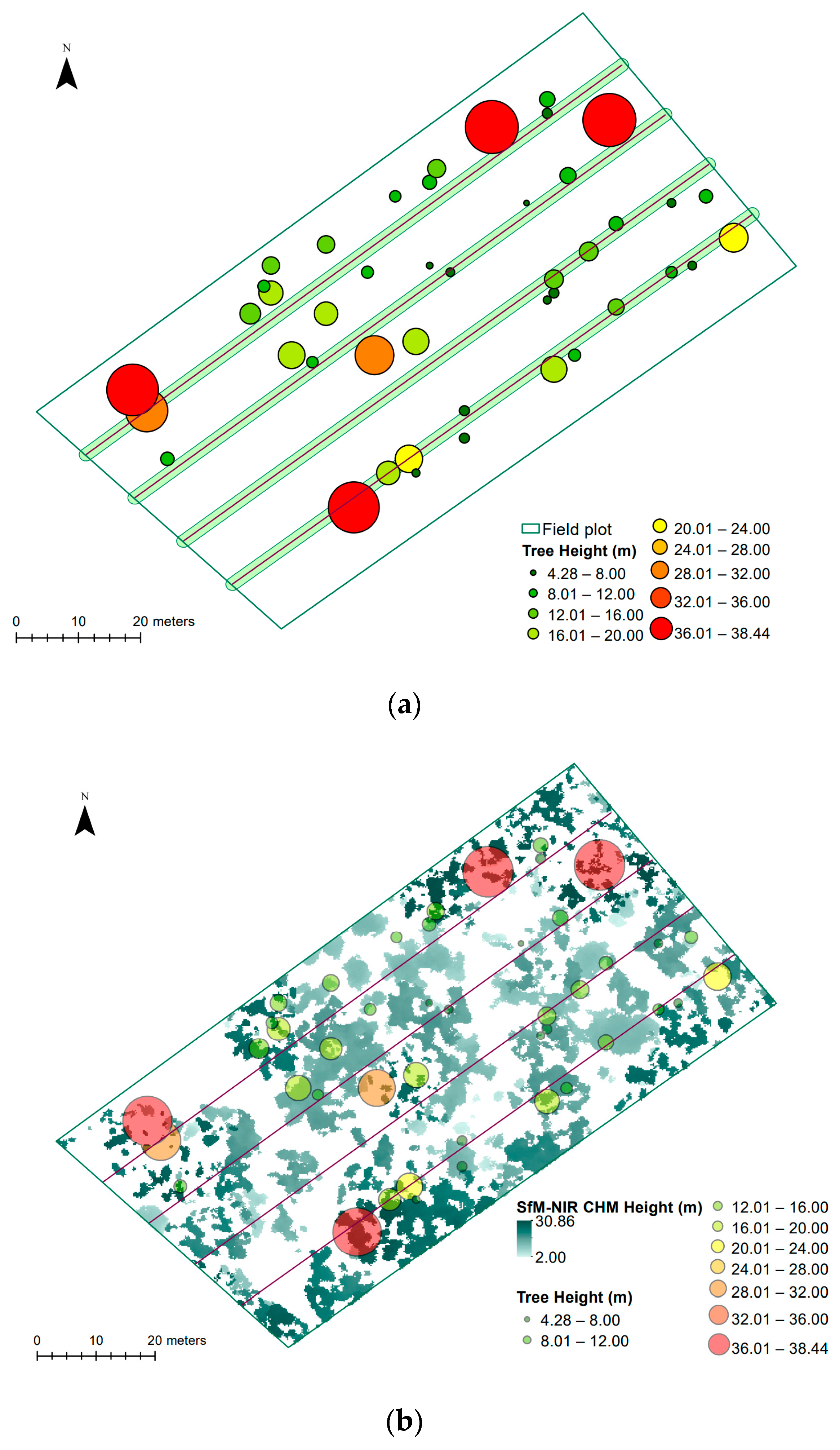
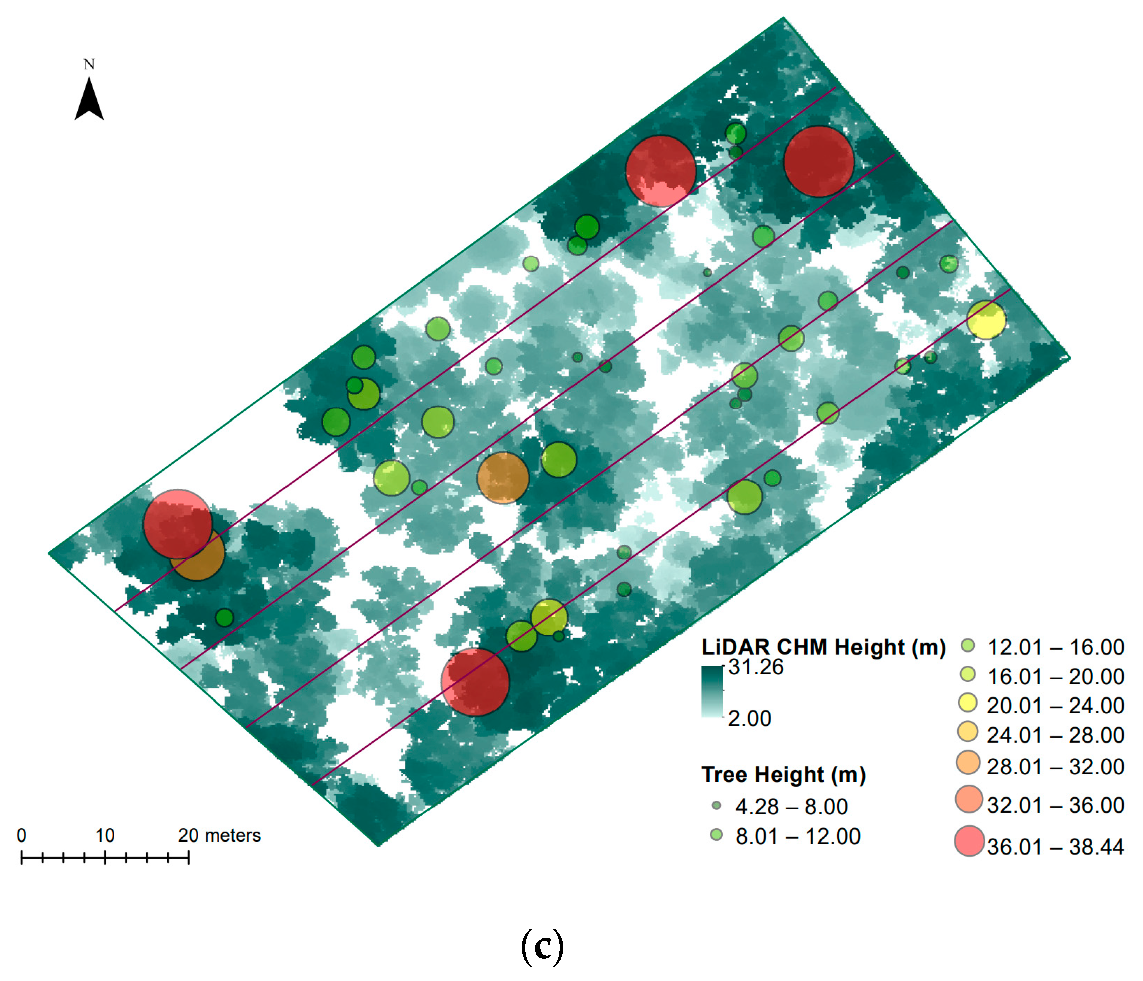
Field-measured heights of trees with DBH > 0.2 m (n = 45) ranged from 4.28 m to 38.44 m (mean = 14.41+/−9.35 (1 SD) m) (Figure 11a). Three of the measured trees were taller than the maximum CHM heights. CHM heights at the location of each measured tree ranged from 10.04 m to 29.24 m (mean = 18.57 +/− 6.57 (1 SD) m) for SfM-NIR, and 5.84 m to 30.93 m (mean = 18.86+/−6.92 (1 SD) m) for LiDAR. Figure 11b,c shows the field-measured heights in relation to CHM heights.
Percentile values (Appendix D) were calculated to compare CHM heights at the location of each field-measured tree. Lower percentile values were notably higher for SfM-NIR (p05 = 9.20 m; p10 = 10.45 m) than for LiDAR (p05 = 6.91 m; p10 = 9.20 m). The upper percentile values were only slightly higher for LiDAR (p90 = 28.06 vs. 27.55 m; p95 = 29.64 vs. 28.84 m). The greatest difference occurred at p0 (SfM-NIR + 4.2 m). The full dataset is available in Supplementary Material Table S3.
3.6. Regression Analysis
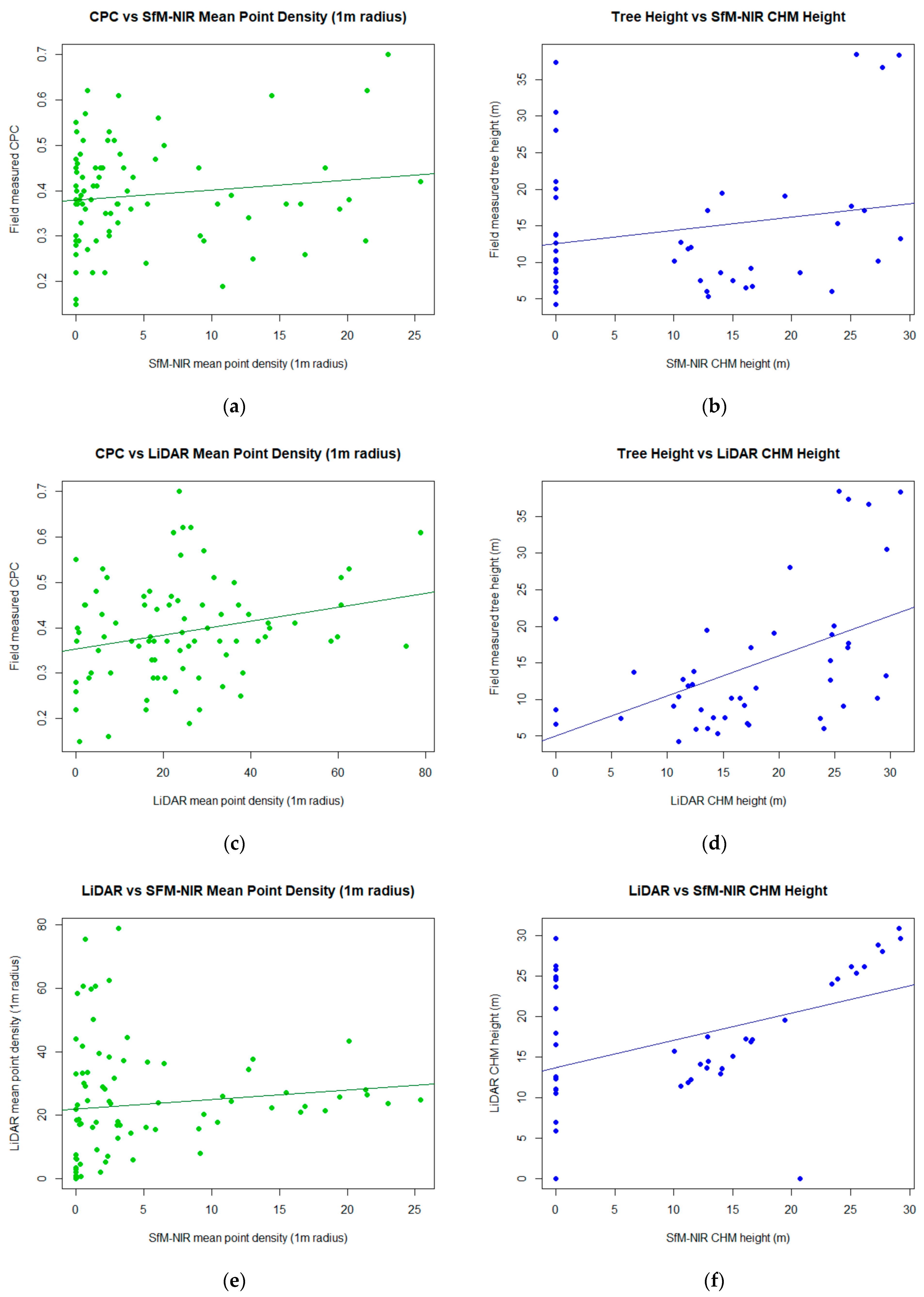
The regression of CPC- and CHM-extracted point densities (Figure 12a,c,e) showed very low correlation between CPC and CHM densities (R2 = 0.0180~SfM-NIR; R2 = 0.0628~LiDAR) and even lower correlation between CHMs (R2 = 0.0121). Figure 12a,e suggests the SfM-NIR dataset is strongly skewed by a high number of zero and near-zero values. The skew is compounded by the fact that many of these zero and near-zero locations correspond to high CPC and LiDAR density values.
Similar relationships were evident in the height data (Figure 12b,d,f) with field-measured height very poorly correlated with CHM height (~SfM-NIR R2 = 0.0415, ~LiDAR R2 = 0.2508) and a low correlation between CHMs (R2 = 0.1712). SfM-NIR height data were again strongly skewed by zero values (n = 20), where field-measured trees corresponded with empty cells in the CHM. Figure 12b suggests that excluding the SfM-NIR zero values would have resulted in a strong correlation with LiDAR heights at the remaining locations. The large number of zero values inflated the RMSE of SfM-NIR predicted heights (13.08 m) and created a negative bias (−4.09 m). The LiDAR CHM predicted tree heights were somewhat closer to field-measured heights (RMSE = 9.29 m), with a bias that suggested the heights were overestimated (2.77 m).
4. Discussion
This study has undertaken a range of comparisons to gain some insight into the accuracy and completeness of UAV-derived DPCs while acknowledging that comparisons based on individual structural parameters do not address broader questions of quality [1]. Comparisons were first made between UAV-SfM-NIR and UAV-LiDAR CHMs to assess differences in height and density distribution and extent. CHM height and density metrics were then compared with field-measured tree heights and CPC. Due to the very obvious difference in canopy penetration and subsequent data capture, this discussion will treat the LiDAR CHM as a surrogate baseline for SfM-NIR CHM assessment and focus strongly on the factors that impeded greater completeness in the SfM-NIR reconstruction.
4.1. Canopy Height Models
The range and distribution of heights were similar in both CHMs, particularly in the higher percentiles, with lower standard deviation in SfM-NIR height, which is consistent with the findings of [14], but LiDAR point density was an order of magnitude greater than SfM-NIR. LiDAR also produced a far greater extent and more connectivity in cover, which could be interpreted as a more complete representation of the canopy when referenced against aerial photographs. Successful SfM reconstruction of woody vegetation such as eucalypt relies on image capture that maximises canopy features [24]. Sub-optimal image matching in the photogrammetric pipeline may have contributed to the sparseness of the SfM-NIR cover, as pre-processing presents challenges that can cause missed objects and vertical bias [14]. Fewer feature matches result in lower 3D point cloud density, which reduces canopy sampling [5].
4.1.1. Effect of Eucalypt Forest Structure
Native eucalypt forests have distinct characteristics that make photogrammetric image matching difficult. This results, in part, from the clumped overstorey structure [25] as photogrammetric reconstruction is far more accurate in continuous cover [19]. Gaps in eucalypt canopies have steep and complex surfaces [24]. These abrupt vertical changes, in combination with highly varied canopy relief, cause omissions that interfere with image matching [19]. Fluttering leaves and swaying branches, which are characteristic of eucalypt forest, can also impair feature matching and reduce SfM point cloud density [5,54]. Canopy movement is a possible explanation for the unexpectedly low proportion of SfM-NIR capture in the upper canopy, where only 46% of the data were collected, compared to 54% in the mid-canopy.
4.1.2. Overlap and Spatial Resolution
The quality of SfM reconstructions is improved by high image overlap and ground sampling distance (GSD) >5 cm [1], but spatial resolution is reduced when moving up through the canopy as the distance to the sensor decreases [24]. While the average GSD in the UAV-image survey was 5.2 cm, the average spatial resolution at the base of the CHMs (2 mAGL) was 5.1 cm, with a 105 m × 79 m footprint, ~89% forward lap (70 m) and ~84% side lap (86 m). However, at top-of-canopy height (TCH) (~35 m), the footprint was further reduced to 76 m × 57 m, resulting in ~84% forward lap (48 m), ~78% side lap (59 m) and a spatial resolution of 3.7 cm. This reduced the opportunity for feature matching in the upper canopy by almost half, as single features may have appeared in 48 images at 2 mAGL but in only 25 images at TCH. It is also possible that the default ‘8 matching neighbours’ pre-processing setting in ODM was too low, particularly with image overlap of around 80%, as this combination causes valid matches to be ignored, which decreases reconstruction accuracy [55].
4.1.3. Canopy Penetration
Differences in canopy penetration will have contributed to differences in SfM-NIR and LiDAR CHM height and density metrics [5]. Photogrammetric reconstructions represent the uppermost visible surface rather than the broader range in observed surfaces obtainable with LiDAR [14] and therefore deliver less information on vertical structure [2]. The lack of data in the SfM-NIR ground layer was demonstrated by the lower proportion of points removed when DPCs were trimmed below 2 mAGL. The low SfM-NIR capture from 2 to 10 m, and the lack of trunk representation in the SfM-NIR CHM was consistent with other studies that have observed inadequate SfM capture of mid- and understorey layers [56], often as a result of overstorey occlusion [19]. This problem is exacerbated by the multi-layered eucalypt canopy, such that smaller eucalypt trees are often poorly modelled [24]. The uncharacteristically high proportion of SfM-NIR point capture through the upper–mid-canopy (10–15 m) may have been related to the selection of the NIR spectral band, as NIR has been found to increase point reconstruction in eucalypt canopy [24]. It may also be a product of the large intra-canopy gaps within the eucalypt forest, which would allow a greater penetration than the dense broadleaf canopies that have often been studied [4,19].
4.1.4. Solar Elevation and Shadow
Shadows affect SfM reconstruction. The large brightness differential between a sunlit canopy and areas of shadow reduces feature detectability [2]. It is difficult to avoid the impact of shadows in a mature, native forest [9] where the canopy structure is complex and non-homogenous [57]. Large shadows produced by low solar elevation have been linked to the under-sampling of the canopy surface [5]. To reduce this impact, solar noon is often targeted for remote sensing [6,9,12,24]. However, in native eucalypt forests, low solar elevation surveys (~25°) have been found to improve the reconstruction of canopy features, enhance point reconstruction throughout the vegetation profile and increase useful shadow-based contrast between the ground and canopy, which may be related to the pendulous orientation of eucalypt leaves, such that the leaf surfaces tend to be perpendicular to lower angles [24]. In this study, however, the 33° solar elevation of the UAV-imagery survey was perhaps too large to maximise such enhancements, at least with NIR data alone. In addition, UAV-image surveys flown before solar noon can cause objects that occur to the west of vertical features to be obfuscated [21]. This is particularly apparent in the height and density differences in the north/northeast corner of the CHMs. The effect is likely to have been compounded by shadows cast by the sun at a late-winter 54° azimuth. Solar azimuth should perhaps be incorporated into UAV-imagery flight planning to the same extent as solar elevation. Overall, these shadow effects are perhaps unsurprising, given that single-time-of-day photogrammetry products have been found to produce sub-optimal results in native eucalypt forests [24]. On this basis, it is considered that a single NIR survey was insufficient to gain full insight into the contribution of NIR data and that multiple UAV-image surveys should be conducted at different solar elevations and combined [21,24]. In addition, it may be beneficial to fly UAV-image surveys closer to a solar equinox.
4.2. CHM Comparison with Field Measurements
While the SfM-NIR CHM produced less cover and lower point densities than the LiDAR CHM, this does not necessarily translate to less accuracy. To gain some insight into the performance of the models as representative reconstructions, a comparison with field data was necessary.
4.2.1. Canopy Cover
Extracted SfM-NIR point density data was strongly skewed by empty cells, and LiDAR demonstrated high point density at many locations where SfM-NIR point density was zero or near zero. The correlation between extracted CHM point densities and field-measured CPC was very low. These results are perhaps unsurprising. LiDAR point density has been found to be an unreliable proxy for canopy cover as it is highly inconsistent across the point cloud [2] and strongly affected by survey altitude [58]. Point cloud density in SfM reconstructions may also be considered an unreliable proxy, as it is impacted by many factors in the field unrelated to canopy cover, such as spatial resolution, wind, shadow and movement, as well as feature matching challenges presented by the photogrammetric pipeline [5]. The patchy nature of the eucalypt canopy may also have been a source of error as CPC varied widely, with no discernible pattern across the field plot. As a result, the extracted CHM density values (1 m radius) are unlikely to have provided precise samples.
4.2.2. Canopy Height
Comparing UAV-derived data with field-derived measurements, Ref. [58] found that both photogrammetric and LiDAR DPC reconstructions overestimated tree heights, particularly for tree heights between 21 and 30 metres in intermediate or codominant crown classes. This finding concurs with the LiDAR overestimation and bias (+2.77 m; +0.7%) observed in this study, but not the SfM-NIR underestimation (−4.09 m; −1.1%). The SfM-NIR underestimation can be partially explained by incomplete canopy reconstruction, which was driven by an absence of SfM-NIR data at 20 of the 45 measured tree locations. Removal of those 20 datapoints would have increased the SfM-NIR correlation with field measurements from R = 0.2 to 0.6, reduced RMSE from 13.08 to 8.01 m and produced a slightly positive bias (+9.7 × 10⁻¹⁷). The challenges already identified with feature matching may have contributed to missing SfM-NIR data. TCH in remotely sensed CHMs, whether SfM or LiDAR, represents average height across the entire outer surface [5]. Eucalypt characteristics such as canopy movement also cause underestimation of TCH [5], although SfM overestimations have been observed in eucalypt forests [2]. It is also possible that the over/underestimations do not represent CHM error. Field-measured height can incorporate significant error as it is difficult to accurately estimate the treetop from the ground [5].
5. Conclusions
The remotely sensed SfM-NIR and LiDAR DPCs in this study did not produce comparable representations of native dry eucalypt forest canopy, and neither produced a complete reconstruction of the canopy cover. Comparison between CHMs showed the models were similar in their representation of tree heights but varied greatly in relation to CPC and canopy extent. Most notably, SfM-NIR data were missing from many locations where LiDAR data were successfully collected, and all other observed differences appear to have stemmed from this. Comparisons with field-measured data confirmed that the LiDAR DPC reconstruction was more representative of the eucalypt canopy. It appears that a single UAV survey was insufficient to achieve a more complete SfM-NIR canopy reconstruction [24], and it is recommended that multiple surveys be conducted at different solar elevations and combined for future comparative studies in native dry eucalypt forests. Photogrammetric pre-processing settings should also be further explored in an effort to optimise image feature matching. While NIR data on its own was not expected to achieve a complete reconstruction, this study has nonetheless provided some insight into its contribution to native dry eucalypt forest modelling, in addition to assessing the performance of LiDAR for this purpose.
Supplementary Materials
The following supporting information can be downloaded at: https://www.mdpi.com/article/10.3390/rs15061694/s1, Table S1: Default Open Drone Map pre-processing settings; Table S2: Full dataset for CPC and CHM point density at field data points; Table S3: Full dataset for field-measured and corresponding CHM heights.
Author Contributions
Conceptualization, M.W.; methodology, M.W.; formal analysis, M.W.; resources, G.H.; writing—original draft preparation, M.W.; writing—review and editing, M.W. and G.H. All authors have read and agreed to the published version of the manuscript.
Funding
This research received no external funding.
Data Availability Statement
Not applicable.
Acknowledgments
This work was enabled by use of the Queensland University of Technology (QUT) Research Engineering Facility (REF) hosted by the QUT Division of Research. Data collection in the field was assisted by Brianna Deer, Cameron Coombe, Darcy Hayes, Sarah Johnston and Ella Sinclair.
Conflicts of Interest
The authors declare no conflict of interest.
Appendix A
Figure A1.
Raster analysis of the extent of cover in CHMs produced from (a) SfM-NIR and (b) LiDAR. Empty cells are shown in white.
Figure A1.
Raster analysis of the extent of cover in CHMs produced from (a) SfM-NIR and (b) LiDAR. Empty cells are shown in white.


Table A1.
Comparison of extent of cover using SfM-NIR and LiDAR CHMs calculated as the number of empty cells as a proportion of available cells.
Table A1.
Comparison of extent of cover using SfM-NIR and LiDAR CHMs calculated as the number of empty cells as a proportion of available cells.
| Number of Empty Cells | Number of Available Cells | % No Cover | % Cover | |
|---|---|---|---|---|
| SfM-NIR CHM | 72,879 | 269,230 | 27.1 | 72.9 |
| LiDAR CHM | 25,274 | 269,775 | 9.4 | 90.6 |
Appendix B
Table A2.
Distribution in CPC estimates.
| CPC | Sites | % |
|---|---|---|
| 0.15–0.22 | 6 | 7.1 |
| 0.22–0.31 | 17 | 20.2 |
| 0.31–0.37 | 18 | 21.4 |
| 0.37–0.42 | 13 | 15.5 |
| 0.42–0.48 | 16 | 19.0 |
| 0.48–0.57 | 8 | 9.5 |
| 0.57–0.70 | 6 | 7.1 |
| Total | 84 | 100 |
Appendix C
Table A3.
Percentile values for CPC and CHM point density at field data collection points (n = 84).
| Field Measured CPC/CHM Mean Point Density per 0.2 m Grid Cell (within 1 m Radius) | ||||||||||
|---|---|---|---|---|---|---|---|---|---|---|
| Mean+/−1 SD | p0 | p05 | p10 | p25 | p50 | p75 | p90 | p95 | p100 | |
| Field CPC | 0.39+/−0.11 | 0.15 | 0.22 | 0.26 | 0.30 | 0.38 | 0.45 | 0.53 | 0.60 | 0.70 |
| SfM-NIR CHM mean point density | 4.74+/−6.61 | 0.00 | 0.00 | 0.00 | 0.18 | 1.89 | 5.90 | 16.23 | 20.05 | 25.41 |
| LiDAR CHM mean point density | 23.37+/−18.13 | 0.00 | 0.00 | 0.71 | 7.75 | 22.04 | 33.04 | 44.24 | 60.57 | 78.92 |
Appendix D
Table A4.
Percentile values for field-measured and corresponding CHM heights (n = 45).
| Field Measured Tree Height (m)/CHM Height at Same Location (m) | ||||||||||
|---|---|---|---|---|---|---|---|---|---|---|
| Mean+/−1 SD | p0 | p05 | p10 | p25 | p50 | p75 | p90 | p95 | p100 | |
| Field tree height | 14.41+/−9.35 | 4.28 | 5.95 | 6.21 | 7.55 | 11.55 | 17.65 | 29.55 | 37.19 | 38.44 |
| SfM-NIR CHM height | 18.57+/−6.57 | 10.04 | 10.71 | 11.31 | 12.88 | 16.56 | 25.08 | 27.55 | 28.84 | 29.24 |
| LiDAR CHM height | 18.86+/−6.92 | 5.84 | 10.53 | 11.04 | 12.99 | 17.29 | 24.98 | 28.06 | 29.64 | 30.93 |
References
- Frey, J.; Kovach, K.; Stemmler, S.; Koch, B. UAV photogrammetry of forests as a vulnerable process. A sensitivity analysis for a structure from motion RGB-image pipeline. Remote Sens. 2018, 10, 912. [Google Scholar] [CrossRef] [Green Version]
- Wallace, L.; Lucieer, A.; Malenovsky, Z.; Turner, D.; Vopenka, P. Assessment of forest structure using two UAV techniques: A comparison of airborne laser scanning and structure from motion (SfM) point clouds. Forests 2016, 7, 62. [Google Scholar] [CrossRef] [Green Version]
- Fortin, J.A.; Cardille, J.A.; Perez, E. Multi-sensor detection of forest-cover change across 45 years in Mato Grosso, Brazil. Remote Sens. Environ. 2020, 238, 111266. [Google Scholar] [CrossRef]
- Sunde, M.G.; Diamond, D.D.; Elliott, L.F.; Hanberry, P.; True, D. Mapping high-resolution percentage canopy cover using a multi-sensor approach. Remote Sens. Environ. 2020, 242, 111748. [Google Scholar] [CrossRef]
- Dandois, J.P.; Olano, M.; Ellis, E.C. Optimal altitude, overlap, and weather conditions for computer vision UAV estimates of forest structure. Remote Sens. 2015, 7, 13895–13920. [Google Scholar] [CrossRef] [Green Version]
- Hernandez-Santin, L.; Rudge, M.L.; Bartolo, R.E.; Erskine, P.D. Identifying species and monitoring understorey from UAS-derived data: A literature review and future directions. Drones 2019, 3, 9. [Google Scholar] [CrossRef] [Green Version]
- Morley, P.J.; Donoghue, D.N.M.; Chen, J.-C.; Jump, A.S. Quantifying structural diversity to better estimate change at mountain forest margins. Remote Sens. Environ. 2019, 223, 291–306. [Google Scholar] [CrossRef]
- Puliti, S.; Dash, J.P.; Watt, M.S.; Breidenbach, J.; Pearse, G.D. A comparison of UAV laser scanning, photogrammetry and airborne laser scanning for precision inventory of small-forest properties. Forestry 2019, 93, 150–162. [Google Scholar] [CrossRef]
- Guerra-Hernandez, J.; Cosenza, D.N.; Rodriguez, L.C.E.; Silva, M.; Tomé, M.; Díaz-Varela, R.A.; González-Ferreiro, E. Comparison of ALS- and UAV(SfM)-derived high-density point clouds for individual tree detection in eucalyptus plantations. Int. J. Remote Sens. 2018, 39, 5211–5235. [Google Scholar] [CrossRef]
- Ganz, S.; Kaber, Y.; Adler, P. Measuring tree height with remote sensing–A comparison of photogrammetric and LiDAR data with different field measurements. Forests 2019, 10, 694. [Google Scholar] [CrossRef] [Green Version]
- Davies, A.B.; Asner, G.P. Advances in animal ecology from 3D-LiDAR ecosystem mapping. Trends Ecol. Evol. 2014, 29, 681–691. [Google Scholar] [CrossRef] [PubMed]
- Iglhaut, J.; Puliti, S.; Piermattei, L.; O’Connor, J.; Rosette, J. Structure from motion photogrammetry in forestry: A review. Curr. For. Rep. 2019, 5, 155–168. [Google Scholar] [CrossRef] [Green Version]
- Tickle, P.K.; Lee, A.C.; Lucas, R.M.; Austin, J.M.; Witte, C. Quantifying Australian forest floristics and structure using small footprint LiDAR and large scale aerial photography. For. Ecol. Manag. 2006, 223, 379–394. [Google Scholar] [CrossRef]
- Filippelli, S.K.; Lefsky, M.A.; Rocca, M.E. Comparison and integration of lidar and photogrammetric point clouds for mapping pre-fire forest structure. Remote Sens. Environ. 2019, 224, 154–166. [Google Scholar] [CrossRef]
- Fisher, A.; Armston, J.; Goodwin, N.; Scarth, P. Modelling canopy gap probability, foliage projective cover and crown projective cover from airborne lidar metrics in Australian forests and woodlands. Remote Sens. Environ. 2020, 237, 111520. [Google Scholar] [CrossRef]
- Kellner, J.R.; Armston, J.; Birrer, M.; Cushman, K.C.; Duncanson, L.; Eck, C.; Falleger, C.; Imbach, B.; Král, K.; Krůček, M.; et al. New opportunities for forest remote sensing through ultra-high-density drone lidar. Surv. Geophys. 2019, 40, 959–977. [Google Scholar] [CrossRef] [Green Version]
- Remondino, F.; Nocerino, E.; Toschi, I.; Menna, F. A critical review of automated photogrammetric processing of large datasets. Int. Arch. Photogramm. Remote Sens. Spatial Inf. Sci. 2017, 42, 591–599. [Google Scholar] [CrossRef] [Green Version]
- Gianetti, F.; Puletti, N.; Puliti, S.; Travaglini, D.; Chirici, G. Assessment of UAV photogrammetric DTM-independent variables for modelling and mapping forest structural indices in mixed temperate forests. Ecol. Indic. 2020, 117, 106513. [Google Scholar] [CrossRef]
- Lisein, J.; Pierrot-Deseilligny, M.; Bonnet, S.; Lejune, P. A photogrammetric workflow for the creation of a forest canopy height model from small unmanned aerial system imagery. Forests 2013, 4, 922–944. [Google Scholar] [CrossRef] [Green Version]
- Poorazimy, M.; Shataee, S.; McRoberts, R.E.; Mohammadi, J. Integrating airborne laser scanning data, space-borne radar data and digital aerial imagery to estimate aboveground carbon stock in Hyrcanian forests, Iran. Remote Sens. Environ. 2020, 240, 111669. [Google Scholar] [CrossRef]
- Rahman, M.M.; McDermid, G.J.; Mckeeman, T.; Lovitt, J. A workflow to minimize shadows in UAV-based orthomosaics. J. Unmanned Veh. Syst. 2019, 7, 107–117. [Google Scholar] [CrossRef]
- Ecke, S.; Dempewolf, J.; Frey, J.; Schwaller, A.; Endres, E.; Klemmt, H.-J.; Tiede, D.; Seifert, T. UAV-based forest health monitoring: A systematic review. Remote Sens. 2022, 14, 3205. [Google Scholar] [CrossRef]
- Hillman, S.; Hally, B.; Wallace, L.; Turner, D.; Lucieer, A.; Reinke, K.; Jones, S. High-resolution estimates of fire severity—An evaluation of uas image and lidar mapping approaches on a sedgeland forest boundary in Tasmania, Australia. Fire 2021, 4, 14. [Google Scholar] [CrossRef]
- Fletcher, A.; Mather, R. Hypertemporal imaging capability of UAS improves photogrammetric tree canopy models. Remote Sens. 2020, 12, 1238. [Google Scholar] [CrossRef] [Green Version]
- Goldbergs, G.; Maier, S.W.; Levick, S.R.; Edwards, A. Limitations of high resolution satellite stereo imagery for estimating canopy height in Australian tropical savannas. Int. J. Appl. Earth Obs. 2019, 75, 83–95. [Google Scholar] [CrossRef]
- Queensland Government. Eucalypt Open-Forest. Available online: https://www.qld.gov.au/environment/plants-animals/habitats/habitat/eucalypt-open-forest (accessed on 31 January 2023).
- Olive, K.; Lewis, T.; Ghaffariyan, M.R.; Srivastava, S.K. Comparing canopy height estimates from satellite-based photogrammetry, airborne laser scanning and field measurements across Australian production and conservation eucalypt forests. J. For. Res. Jpn. 2020, 25, 108–112. [Google Scholar] [CrossRef]
- Corte, A.P.D.; de Vasconcellos, B.N.; Rex, F.E.; Sanquetta, C.R.; Mohan, M.; Silva, C.A.; Klauberg, C.; de Almeida, D.R.A.; Zambrano, A.M.A.; Trautenmüller, J.W.; et al. Applying high-resolution uav-lidar and quantitative structure modelling for estimating tree attributes in a crop-livestock-forest system. Land 2022, 11, 507. [Google Scholar] [CrossRef]
- Gao, L.; Chai, G.; Zhang, X. Above-ground biomass estimation of plantation with different tree species using airborne lidar and hyperspectral data. Remote Sens. 2022, 14, 2568. [Google Scholar] [CrossRef]
- Liao, K.; Li, Y.; Zou, B.; Li, D.; Lu, D. Examining the role of uav lidar data in improving tree volume calculation accuracy. Remote Sens. 2022, 14, 4410. [Google Scholar] [CrossRef]
- Silva, C.A.; Klauberg, C.; Hudak, A.T.; Vierling, L.A.; Liesenberg, V.; Carvalho, S.P.C.E.; Rodriguez, L.C.E. A principal component approach for predicting the stem volume in eucalyptus plantations in Brazil using airborne lidar data. Int. J. For. Res. 2016, 89, 422–433. [Google Scholar] [CrossRef] [Green Version]
- Silva, C.A.; Klauberg, C.E.; Carvalho, S.D.P.C.; Hudak, A.T.; Rodriguez, L.C.E. Mapping Aboveground Carbon Stocks Using Lidar Data in Eucalyptus spp. Plantations in the State of São Paulo, Brazil. Sci For. 2014, 42, 591–604. Available online: https://www.scopus.com/inward/record.uri?eid=2-s2.0-84923204323&partnerID=40&md5=080c779b8162dc1b043d3b8542c42ee9 (accessed on 2 February 2023).
- Zhang, Y.; Lu, D.; Jiang, X.; Li, Y.; Li, D. Forest structure simulation of eucalyptus plantation using remote-sensing-based forest age data and 3-pg model. Remote Sens. 2023, 15, 183. [Google Scholar] [CrossRef]
- Karna, Y.K.; Penman, T.D.; Aponte, C.; Gutekunst, C.; Bennett, L.T. Indications of positive feedbacks to flammability through fuel structure after high-severity fire in temperate eucalypt forests. Int. J. Wildland Fire 2021, 30, 664–679. [Google Scholar] [CrossRef]
- Brown, T.P.; Inbar, A.; Duff, T.J.; Burton, J.; Noske, P.J.; Lane, P.N.J.; Sheridan, G.J. Forest structure drives fuel moisture response across alternative forest states. Fire 2021, 4, 48. [Google Scholar] [CrossRef]
- Pendall, E.; Hewitt, A.; Boer, M.M.; Carrillo, Y.; Glenn, N.F.; Griebel, A.; Middleton, J.H.; Mumford, P.J.; Ridgeway, P.; Rymer, P.D.; et al. Remarkable resilience of forest structure and biodiversity following fire in the peri-urban bushland of Sydney, Australia. Climate 2022, 10, 86. [Google Scholar] [CrossRef]
- Fedrigo, M.; Newnham, G.J.; Coops, N.C.; Culvenor, D.S.; Bolton, D.K.; Nitschke, C.R. Predicting temperate forest stand types using only structural profiles from discrete return airborne lidar. ISPRS J. Photogramm. Remote Sens. 2018, 136, 106–119. [Google Scholar] [CrossRef]
- Jaskierniak, D.; Lucieer, A.; Kuczera, G.; Turner, D.; Lane, P.N.J.; Benyon, R.G.; Haydon, S. Individual tree detection and crown delineation from unmanned aircraft system (uas) lidar in structurally complex mixed species eucalypt forests. ISPRS J. Photogramm. 2021, 171, 171–187. [Google Scholar] [CrossRef]
- Trouvé, R.; Jiang, R.; Fedrigo, M.; White, M.D.; Kasel, S.; Baker, P.J.; Nitschke, C.R. Combining environmental, multispectral, and lidar data improves forest type classification: A case study on mapping cool temperate rainforests and mixed forests. Remote Sens. 2023, 15, 60. [Google Scholar] [CrossRef]
- Dhargay, S.; Lyell, C.S.; Brown, T.P.; Inbar, A.; Sheridan, G.J.; Lane, P.N.J. Performance of gedi space-borne lidar for quantifying structural variation in the temperate forests of south-eastern Australia. Remote Sens. 2022, 14, 3615. [Google Scholar] [CrossRef]
- Fisher, A.; Scarth, P.; Armston, J.; Danaher, T. Relating foliage and crown projective cover in Australian tree stands. Agr. Forest Meteorol. 2018, 259, 39–47. [Google Scholar] [CrossRef]
- Almeida, A.; Gonçalves, F.; Silva, G.; Mendonça, A.; Gonzaga, M.; Silva, J.; Souza, R.; Leite, I.; Neves, K.; Boeno, M.; et al. Individual tree detection and qualitative inventory of a Eucalyptus sp. stand using uav photogrammetry data. Remote Sens. 2021, 13, 3655. [Google Scholar] [CrossRef]
- Dell, M.; Stone, C.; Osborn, J.; Glen, M.; McCoull, C.; Rimbawanto, A.; Tjahyono, B.; Mohammed, C. Detection of necrotic foliage in a young Eucalyptus pellita plantation using unmanned aerial vehicle RGB photography–a demonstration of concept. Aust. For. 2019, 82, 79–88. [Google Scholar] [CrossRef] [Green Version]
- Tupinambá-Simões, F.; Bravo, F.; Guerra-Hernández, J.; Pascual, A. Assessment of drought effects on survival and growth dynamics in eucalypt commercial forestry using remote sensing photogrammetry. A showcase in Mato Grosso, Brazil. Forest Ecol. Manag. 2022, 505, 119930. [Google Scholar] [CrossRef]
- Zhu, R.; Guo, Z.; Zhang, X. Forest 3d reconstruction and individual tree parameter extraction combining close-range photo enhancement and feature matching. Remote Sens. 2021, 13, 1633. [Google Scholar] [CrossRef]
- Krisanski, S.; Taskhiri, M.S.; Turner, P. Enhancing methods for under-canopy unmanned aircraft system based photogrammetry in complex forests for tree diameter measurement. Remote Sens. 2020, 12, 1652. [Google Scholar] [CrossRef]
- Queensland Government. Regional Ecosystem Details for 12.12.12. Available online: https://apps.des.qld.gov.au/regional-ecosystems/details/?re=12.12.12 (accessed on 11 September 2020).
- Vélez, S.; Vacas, R.; Martín, H.; Ruano-Rosa, D.; Álvarez, S. A novel technique using planar area and ground shadows calculated from UAV RGB imagery to estimate pistachio tree (Pistacia vera L.) canopy volume. Remote Sens. 2022, 14, 6006. [Google Scholar] [CrossRef]
- Kükenbrink, D.; Marty, M.; Bösch, R.; Ginzler, C. Benchmarking laser scanning and terrestrial photogrammetry to extract forest inventory parameters in a complex temperate forest. Int. J. Appl. Earth Obs. 2022, 113, 102999. [Google Scholar] [CrossRef]
- Brede, B.; Terryn, L.; Barbier, N.; Bartholomeus, H.M.; Bartolo, R.; Calders, K.; Derroire, G.; Krishna Moorthy, S.M.; Lau, A.; Levick, S.R.; et al. Non-destructive estimation of individual tree biomass: Allometric models, terrestrial and UAV laser scanning. Remote Sens. Environ. 2022, 280, 113180. [Google Scholar] [CrossRef]
- Patel, N. CanopyCapture (Version 1.0.2) [Mobile Application Software]. Available online: https://nikp29.github.io/CanopyCapture/ (accessed on 25 August 2020).
- Thiel, C.; Schmullius, C. Comparison of UAV photograph-based and airborne lidar-based point clouds over forest from a forestry application perspective. Int. J. Remote Sens. 2017, 38, 241–2426. [Google Scholar] [CrossRef]
- Whitehurst, A.S.; Swatantran, A.; Blair, J.B.; Hofton, M.A.; Dubayah, R. Characterization of canopy layering in forested ecosystems using full waveform lidar. Remote Sens. 2013, 5, 2014–2036. [Google Scholar] [CrossRef] [Green Version]
- Whiteside, T.; Bartolo, R. A robust object-based woody cover extraction technique for monitoring mine site revegetation at scale in the monsoonal tropics using multispectral RPAS imagery from different sensors. Int. J. Appl. Earth Obs. 2018, 73, 300–312. [Google Scholar] [CrossRef]
- Toffanin, P. OpenDroneMap: The Missing Guide: A Practical Guide to Drone Mapping Using Free and Open Source Software, 1st ed.; UAV4GEO: St. Petersburg, FL, USA, 2019. [Google Scholar]
- Goldbergs, G.; Maier, S.W.; Levick, S.R.; Edwards, A. Efficiency of individual tree detection approaches based on light-weight and low-cost UAS imagery in Australian savannas. Remote Sens. 2018, 10, 161. [Google Scholar] [CrossRef] [Green Version]
- Sofonia, J.J.; Phinn, S.; Roelfsema, C.; Kendoul, F.; Rist, Y. Modelling the effects of fundamental UAV flight parameters on LiDAR point clouds to facilitate objectives-based planning. ISPRS J. Photogramm. 2019, 149, 105–118. [Google Scholar] [CrossRef]
- Jurjević, L.; Liang, X.; Gašparović, M.; Balenović, I. Is field-measured tree height as reliable as believed–Part II, A comparison study of tree height estimates from conventional field measurement and low-cost close-range remote sensing in a deciduous forest. ISPRS J. Photogramm. 2020, 169, 227–241. [Google Scholar] [CrossRef]
Figure 1.
Location and characteristics of the study site at Samford Ecological Research Facility in Brisbane, Queensland. The inset at the top left shows the location of Brisbane relative to the whole of Australia. The embedded images at the bottom left show the appearance of the vegetation in the field plot looking across the landscape and up into the canopy.

Figure 2.
The extent of the point cloud generated using the UAV-LiDAR survey is depicted above in yellow. The red polygon shows the location of the field plot within the point cloud and the green line represents the flight path which comprised a perpendicular grid with 30 m spacing.
Figure 2.
The extent of the point cloud generated using the UAV-LiDAR survey is depicted above in yellow. The red polygon shows the location of the field plot within the point cloud and the green line represents the flight path which comprised a perpendicular grid with 30 m spacing.

Figure 3.
This image depicts the landscape surrounding the study site with the UAV flight path used to collect digital imagery (comprising 16 survey lines with 19 m spacing) shown in blue. The red area shows the location of the field plot within this survey area.
Figure 3.
This image depicts the landscape surrounding the study site with the UAV flight path used to collect digital imagery (comprising 16 survey lines with 19 m spacing) shown in blue. The red area shows the location of the field plot within this survey area.

Figure 4.
The 50 m × 100 m field plot (orange outline) is shown with a data strip extending 1 m on either side of four transects set 10 m apart (shown in yellow). Data was collected at 5-metre intervals along each transect (orange asterisks).
Figure 4.
The 50 m × 100 m field plot (orange outline) is shown with a data strip extending 1 m on either side of four transects set 10 m apart (shown in yellow). Data was collected at 5-metre intervals along each transect (orange asterisks).

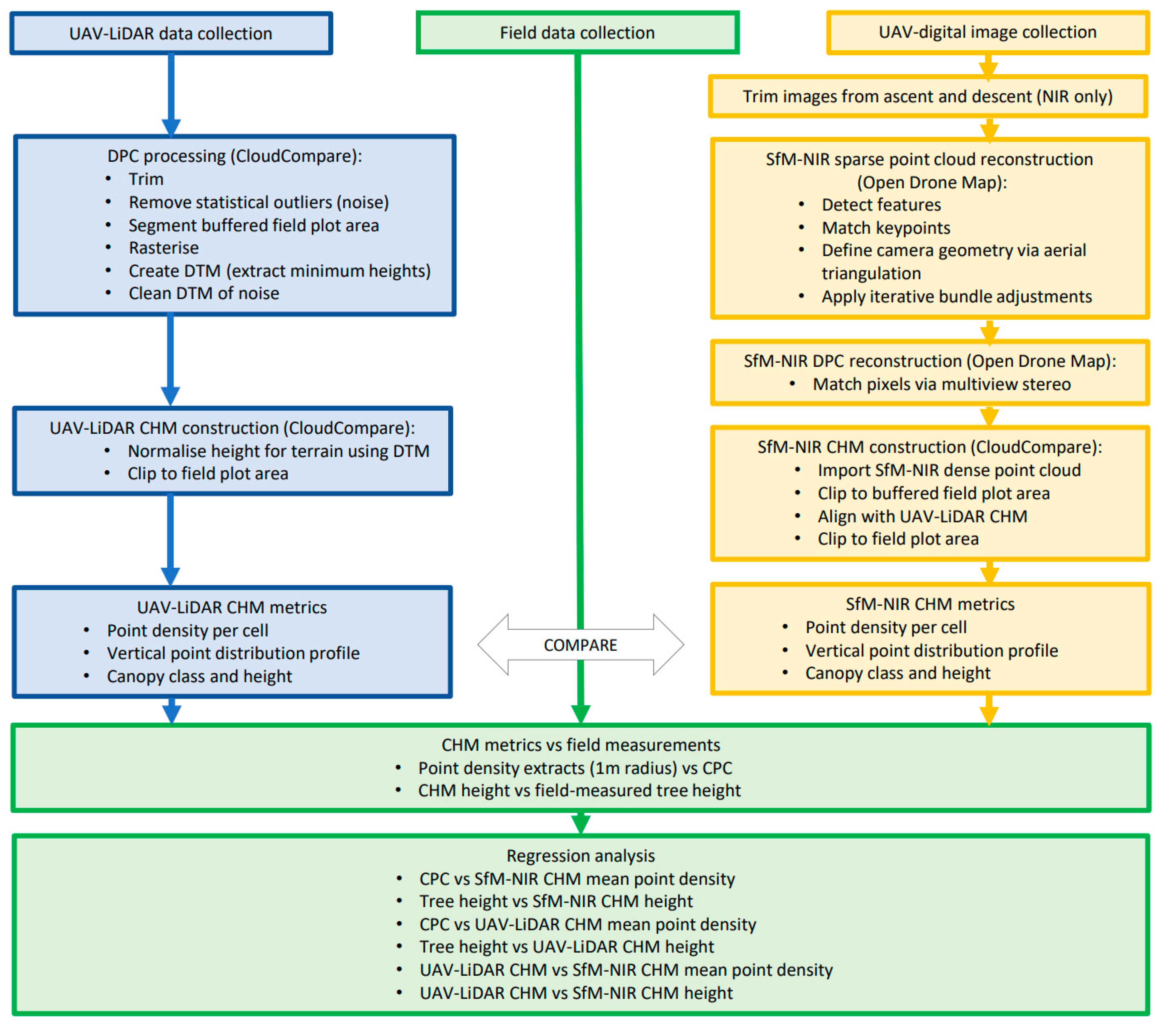
Figure 5.
The workflow for LiDAR and NIR data collection, point cloud processing and CHM reconstruction, followed by analysis involving comparison between CHM metrics and against field-derived measurements.
Figure 5.
The workflow for LiDAR and NIR data collection, point cloud processing and CHM reconstruction, followed by analysis involving comparison between CHM metrics and against field-derived measurements.

Figure 6.
Point density values (per cell) are shown for the (a) SfM-NIR CHM and (b) LiDAR CHM. (c) The difference in point density distributions with the SfM-NIR CHM (dark to light grey) overlaid on the LiDAR CHM (red to green), highlighting not only the higher density of the LiDAR CHM but also the gaps in SfM-NIR data. The white areas represent points at which no data were collected.


Figure 7.
Above-ground height distribution of points in each CHM showing SfM-NIR in green and LiDAR in red. The frequency percentage on the y-axis represents the number of points collected at each height as a proportion of the total number of points collected with each sensor.
Figure 7.
Above-ground height distribution of points in each CHM showing SfM-NIR in green and LiDAR in red. The frequency percentage on the y-axis represents the number of points collected at each height as a proportion of the total number of points collected with each sensor.

Figure 8.
Visual comparison of CHMs in CloudCompare showed the difference between the SfM-NIR and LiDAR height distribution in (a,b) plan view and (c,d) elevation view (scale bar in metres). The elevation view shows the colour gradation from blue (lowest) to red (highest) height.
Figure 8.
Visual comparison of CHMs in CloudCompare showed the difference between the SfM-NIR and LiDAR height distribution in (a,b) plan view and (c,d) elevation view (scale bar in metres). The elevation view shows the colour gradation from blue (lowest) to red (highest) height.

Figure 9.
Canopy heights and height classes are shown for the (a) SfM-NIR CHM and (b) LiDAR CHM. (c) The difference in the distribution of height classes with the SfM-NIR CHM (dark to light grey) overlaid on the LiDAR CHM (red to green).
Figure 9.
Canopy heights and height classes are shown for the (a) SfM-NIR CHM and (b) LiDAR CHM. (c) The difference in the distribution of height classes with the SfM-NIR CHM (dark to light grey) overlaid on the LiDAR CHM (red to green).

Figure 10.
(a) The measured CPC at each field data collection point, with values ranging from 0.15 (lightest yellow) to 0.70 (darkest blue). These values were compared with the point density per cell within a 1 m radius of each data collection point in the (b) buffered SfM-NIR CHM and (c) buffered LiDAR CHM.


Figure 11.
(a) Map showing the field-measured heights in relation to field plot and buffered transects. Heights and locations of measured trees in relation to the (b) SfM-NIR CHM and (c) LiDAR CHM height distributions.
Figure 11.
(a) Map showing the field-measured heights in relation to field plot and buffered transects. Heights and locations of measured trees in relation to the (b) SfM-NIR CHM and (c) LiDAR CHM height distributions.


Figure 12.
Scatter plots for CPC values vs. mean point density within a 1 m radius of field data points, and field-measured heights vs. CHM heights at the same locations for (a,b) field measurements vs. SfM-NIR CHM, (c,d) field measurements vs. LiDAR CHM and (e,f) LiDAR vs. SfM-NIR CHMs.
Figure 12.
Scatter plots for CPC values vs. mean point density within a 1 m radius of field data points, and field-measured heights vs. CHM heights at the same locations for (a,b) field measurements vs. SfM-NIR CHM, (c,d) field measurements vs. LiDAR CHM and (e,f) LiDAR vs. SfM-NIR CHMs.

Table 1.
The number of points retained/proportion removed in each DPC iteration.
| SfM-NIR | LiDAR | |||
|---|---|---|---|---|
| Number of Points | % Removed from Previous Cloud | Number of Points | % Removed from Previous Cloud | |
| Raw data | 29,910,131 | - | 112,090,335 | - |
| Trimmed and cleaned | - | - | 85,110,874 | 24.07 |
| Clipped by buffered field plot | 1,158,749 | 96.13 | 7,340,689 | 91.38 |
| Points below 2 mAGL removed | 801,306 | 30.85 | 4,918,675 | 32.99 |
| Clipped by field plot (final CHM) | 468,491 | 41.53 | 2,963,676 | 39.75 |
Disclaimer/Publisher’s Note: The statements, opinions and data contained in all publications are solely those of the individual author(s) and contributor(s) and not of MDPI and/or the editor(s). MDPI and/or the editor(s) disclaim responsibility for any injury to people or property resulting from any ideas, methods, instructions or products referred to in the content. |
© 2023 by the authors. Licensee MDPI, Basel, Switzerland. This article is an open access article distributed under the terms and conditions of the Creative Commons Attribution (CC BY) license (https://creativecommons.org/licenses/by/4.0/).
Share and Cite
MDPI and ACS Style
Winsen, M.; Hamilton, G. A Comparison of UAV-Derived Dense Point Clouds Using LiDAR and NIR Photogrammetry in an Australian Eucalypt Forest. Remote Sens. 2023, 15, 1694. https://doi.org/10.3390/rs15061694
AMA Style
Winsen M, Hamilton G. A Comparison of UAV-Derived Dense Point Clouds Using LiDAR and NIR Photogrammetry in an Australian Eucalypt Forest. Remote Sensing. 2023; 15(6):1694. https://doi.org/10.3390/rs15061694
Chicago/Turabian StyleWinsen, Megan, and Grant Hamilton. 2023. "A Comparison of UAV-Derived Dense Point Clouds Using LiDAR and NIR Photogrammetry in an Australian Eucalypt Forest" Remote Sensing 15, no. 6: 1694. https://doi.org/10.3390/rs15061694
Note that from the first issue of 2016, this journal uses article numbers instead of page numbers. See further details here.