Article

Global Water Quality of Inland Waters with Harmonized Landsat-8 and Sentinel-2 Using Cloud-Computed Machine Learning

1
Hydrology and River Basin Management, TUM School of Engineering and Design, Technical University of Munich, 80333 Munich, Germany
2
Department of Physical Geography and Ecosystem Science, Lund University, SE-221 00 Lund, Sweden
*
Author to whom correspondence should be addressed.
Remote Sens. 2023, 15(5), 1390; https://doi.org/10.3390/rs15051390
Submission received: 3 January 2023 / Revised: 22 February 2023 / Accepted: 27 February 2023 / Published: 1 March 2023

Abstract

:
Modeling inland water quality by remote sensing has already demonstrated its capacity to make accurate predictions. However, limitations still exist for applicability in diverse regions, as well as to retrieve non-optically active parameters (nOAC). Models are usually trained only with water samples from individual or local groups of waterbodies, which limits their capacity and accuracy in predicting parameters across diverse regions. This study aims to increase data availability to understand the performance of models trained with heterogeneous databases from both remote sensing and field measurement sources to improve machine learning training. This paper seeks to build a dataset with worldwide lake characteristics using data from water monitoring programs around the world paired with harmonized data of Landsat-8 and Sentinel-2. Additional feature engineering is also examined. The dataset is then used for model training and prediction of water quality at the global scale, time series analysis and water quality maps for lakes in different continents. Additionally, the modeling performance of nOACs are also investigated. The results show that trained models achieve moderately high correlations for SDD, TURB and BOD (R2 = 0.68) but lower performances for TSM and NO3-N (R2 = 0.43). The extreme learning machine (ELM) and the random forest regression (RFR) demonstrate better performance. The results indicate that ML algorithms can process remote sensing data and additional features to model water quality at the global scale and contribute to address the limitations of transferring and retrieving nOAC. However, significant limitations need to be considered, such as calibrated harmonization of water data and atmospheric correction procedures. Moreover, further understanding of the mechanisms that facilitate nOAC prediction is necessary. We highlight the need for international contributions to global water quality datasets capable of providing extensive water data for the improvement of global water monitoring.

1. Introduction

Monitoring water quality of inland waters in different countries is mostly conducted individually by each nation. Global integration of their data is often constrained by a lack of worldwide projects or collaborations [1]. When possible, the countries measure the water quality mainly inside their borders through their monitoring systems and the data are stored locally. Therefore, an important quantity of data that is collected every year is usually not available or is difficult to access for external researchers or international institutions. Currently, there are international projects that aim to homogeneously integrate water quality data from several countries for applications in water resources [2]. However, these programs are in early stages and up to now there no comprehensive and unique sources for global and homogeneous water quality data. At the same time, the global coverage of operational monitoring stations is insufficient or lacks acceptable levels of confidence and precision [1,3,4]. This situation limits considerably the application of current data-driven methods that use big datasets to learn from water quality patterns. Therefore, monitoring water quality remains limited by only conventional analysis such as collection of water samples in the field and laboratory analysis [5,6]. Conventional methods are highly accurate, but also expensive, time demanding and limited in spatial and temporal coverages. Additionally, it is complex to develop a representative understanding of the water quality status in a waterbody from punctual field measurements or limited field campaigns over the course of large periods of time. A solution to increase the scope and capabilities of monitoring water quality is the use of remote sensing data, which contributes to provide data from remote sensors that couple field data and increase the analysis in time and space. International institutions such as the United Nations already encourage the coupling of monitoring systems with remote sensing technologies through its Environment Program [1]. When paired with field data, combined water and remote sensing measurements allow monitoring at a larger scope, since they have the potential to analyze waterbodies at regional or global locations. This is achieved by studying water quality from indicator parameters and dealing with better cost–benefit methods in comparison with the extensive spatial and temporal scales that are analyzed. Several modeling techniques associate remote-sensed signals, mostly in the visible and near-infrared wavelengths (400–900 nm), with the water parameter of interest to derive information of the waterbody. The relationship between optically active constituents (OAC) such as chlorophyll-a (Chl-a), total suspended matter (TSM) and surface radiation arises due to the interaction between the radiation and the OAC through processes such as absorption and scattering [7]. Remote sensing is suited to analyze these relationships because of the high sensitivity in the radiometric resolution of several satellite sensors. As water absorbs within the visible spectrum, low reflectance occurs in the water column in contrast to the high reflectance of land. Therefore, high sensitivity in the spectral sensors is required to detect the slight changes in water reflectance that surpass the absorption of water [8,9]. Currently, sensors such as Landsat-8 OLI and Sentinel-2 MSI are suited to provide remote sensing data for water quality monitoring because of their radiometric and temporal resolutions [10]. While remote-sensing-based models can reproduce the patters and dynamics of key water parameters, it becomes relevant to improve the confidence and accuracy of such methodologies and the data that are provided to calibrate them. From the different approaches developed in the last decades, machine learning algorithms currently offer accurate and precise models for water quality monitoring [11,12,13,14]. Machine learning comprises statistical methods which are able to learn from the data they are provided through iterative processes of error adjustment between training and prediction datasets. The process involves providing data to the selected algorithm which is trained with known or predefined features or objects that allows detection, classification or pattern recognition in semi-automated or automated learning. Methodologies combining machine learning with remote sensing data have been used to successfully model water quality [14,15,16,17,18,19,20,21]. Some algorithms are considered standard for machine learning evaluations, such as support vector machines (SVR) and random forest regression (RFR) [22]. Furthermore, deep learning, a subset of machine learning based on neural networks, has demonstrated higher accuracy than other methodologies used to model water quality such as bio-optical or band/ratio models [13,23,24,25,26]. Due to its novelty, there are still open challenges in the application of machine learning which require further research [24,27,28,29,30].
The availability of paired remote sensing and field water quality data is highly limited because of the independent nature of acquiring both types of data. Monitoring water quality programs in different countries were not designed to take into consideration remote sensing acquisitions or satellite overpasses. Therefore, an important percentage of field data are not feasible to be coupled with remote sensing images [31]. Moreover, remote sensing data originate from multiple instruments with different characteristics. This heterogeneous data, in terms of frequency, spatial and radiometric resolution, demand further data pre-treatment and better machine learning models to reveal meaningful information and may make difficult model transferability. Inherent challenges regarding modeling processes also exist, in particular for deep learning. Yet, a deeper neural network may retrieve more accurate results but at a higher computational cost and with associated risks of overfitting. To determine optimal conditions and parameters of these elements is still a crucial research question [32]. In addition, important water quality parameters such as nutrient concentrations, indicators of oxygen levels or organic compounds are not feasible to be directly retrieved by remote sensing because of their inaction over the spectral response of the water when dissolved, and are therefore known as non-optically active compounds (nOACs). Current research poses the possibilities to determine these parameters on indirect correlations with other optically active components such as chlorophyll-a, turbidity or suspended solids [33]. Finally, due to the nature of machine learning models trained with remote sensing data being inherently empirical, they are expected to be valid mainly in the region from where their training data are originated, and most of these models are applicable only at their specific regions or waterbodies. As these models rely on optical characteristics, which may vary from waterbody to waterbody in complex waters, their transferability is further limited to the origin of their training data. However, a key characteristic of machine learning methodologies is that they learn patterns and behaviors from great amounts of data. Therefore, the existence of a worldwide integrated dataset of water quality and remote sensing data gives the possibility to develop a data-driven approach with the capacity for global estimations of water quality by comprising global lake characteristics in a single dataset. In this study, we aim to create this dataset with the available resources for remote sensing image processing and open-access field water quality measurements. Harmonization of remote sensing data contributes to the increase in data availability by combining remote sensing data from different sensors. A recent example is the harmonization process for Landsat-8 OLI and Sentinel-2 MSI, which have been subject to treatment to homogenize their spectral response and spatial resolution [10,14,34]. This method aims to standardize these differences to produce harmonized datasets that can be used together for various applications such as land cover classification and change detection. This harmonization process represents a significant improvement in multi-temporal and multi-sensor analysis, making it possible to better track changes in the Earth’s surface over time. Despite some processes of the harmonization not being specifically designed for inland waters, such as the 6S atmospheric correction, it is already widely used in remote sensing, showing promise for improving the accuracy of water quality retrievals in the future. Similarly, the results of its usage require caution when being interpreted. Ultimately, the adoption of these methodologies enabled the construction of a global dataset for model development and contributed to understanding the potential of machine learning with increased data availability.
To contribute to clarifying the above challenges, this work aims (i) to gather open-access water quality monitoring datasets of the relevant parameters from different regions in the world for their synergistic use with remote sensing; (ii) to maximize the data availability of coupled field and sensor acquisitions by using an image homogenization process for L8 and S2 and produce harmonized images from both satellites, enabling both sensors to be used synergistically and increasing the size available spectral data; (iii) to build a comprehensive dataset created from the coupling of the global dataset and the harmonized remote sensing products; and (iv) to model relevant water quality parameters using machine learning and validate the use of the developed models for global water quality predictions. In addition, we investigate the results using this dataset and machine learning approaches to understand better the optimal balance between computational demand and retrieved accuracy as well as the possibilities of nOAC direct or indirect retrievals.

2. Materials and Methods

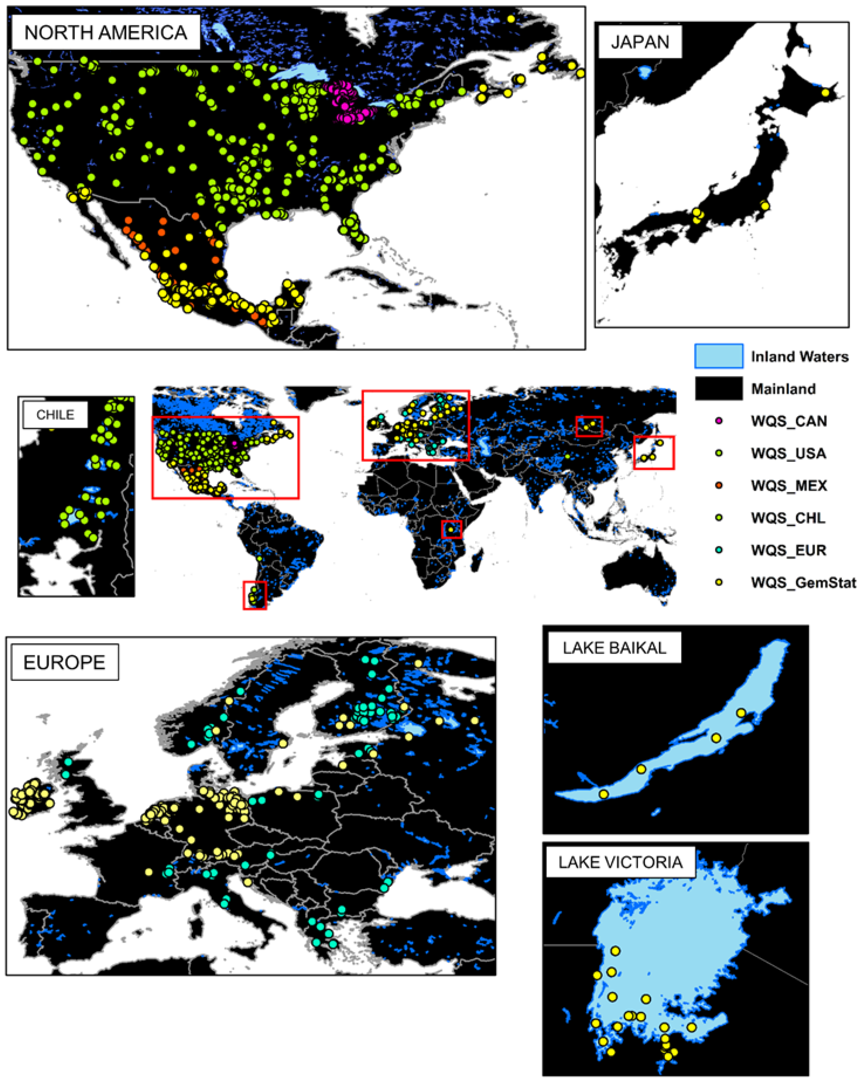
2.1. Sources of Global Water Quality Dataset

The main source of field data is the open-access data portals from water and environment national agencies of different countries which make public their archives of field measurements and monitoring activities. A summary of agencies and links of acquisition is provided in Table 1. In its raw form, the dataset contained almost 300,000 total samples. A summary of the number of observations and lakes by region is displayed in Table 2. The global locations of all the stations from the above-mentioned data sources are shown in Figure 1.
Recent research of Thorslund and van Vliet [35], indicates that the current state of the global water quality stations monitoring lakes and reservoirs is focused mainly on the U.S. followed by Europe, Mexico and South Africa. Australia has a great number of stations, near 90,000, but most of them are for groundwater, and only 5 are located on lakes or reservoirs. For this study, the gross part of the data components comes from the U.S. and European sources since their data archives are open access and easy to acquire through their respective portals. The U.S. data were acquired from the Water Quality Portal [36] (https://www.waterqualitydata.us/, accessed on 15 January 2022), which is a cooperative service sponsored by the United States Geological Survey (USGS), the Environmental Protection Agency (EPA) and the National Water Quality Monitoring Council (NWQMC) that integrates publicly available water quality data from the USGS National Water Information System (NWIS), the EPA STOrage and RETrieval (STORET) Data Warehouse and the USDA ARS Sustaining The Earth’s Watersheds—Agricultural Research Database System (STEWARDS). Data from the European continent were acquired through the European Environment Agency (EEA) Waterbase (https://www.eea.europa.eu/data-and-maps/data/waterbase-water-quality-icm-2, accessed on 13 January 2022), which contains time series of nutrients, organic matter, hazardous substances and other chemicals in rivers, lakes, groundwater and transitional, coastal and marine waters (EEA 2021). Additionally, datasets from the National Water Monitoring Network of Mexico (https://www.gob.mx/conagua/articulos/calidad-del-agua, accessed on 1 September 2021) [37], the Canadian Great Lakes (https://search.open.canada.ca/en/od/, accessed on 15 January 2022) [38], and the Chilean General Water Directory (DGA) lake’s database [39] were also acquired (https://dga.mop.gob.cl/servicioshidrometeorologicos/Paginas/default.aspx, accessed on 15 January 2022). Finally, the Global Freshwater Quality Database (GEMStat) (https://gemstat.org/data/, accessed on 7 January 2022), which is a GEMS/Water Program of the United Nations Environment Program (UNEP), was also acquired to account as much as possible for remaining global data around the world. The GEMStat is hosted by the GEMS/Water Data Centre (GWDC) within the International Centre for Water Resources and Global Change (ICWRGC) in Koblenz, Germany [2].

2.2. Field Dataset Compliance by Lake Selection, Satellite Coincidence and Data Curation

For lake selection, the minimum surface area to consider a waterbody was set to 20 km2. This size ensures the avoidance of adjacency errors in the NIR region from the surrounding land surfaces and bottom reflectance in the sensor acquisitions [40]. At the same time, this area is on the limit to retrieve an adequate number of pixels from the image acquisition based on the spatial resolution per pixel (30 × 30 m) of the intended OLI and MSI sensors to be used as the source of radiometric data.
We used the Level-1 and Level-2 database from the Global Lakes and Wetlands Database (GLWD) developed by the World Wildlife Fund (WWF) and the Center for Environmental Systems Research, University of Kassel, Germany (https://www.worldwildlife.org/pages/global-lakes-and-wetlands-database, accessed on 20 January 2022) [41], to apply lake selection.
The first GLDW product, GLWD-1, comprises 3067 lakes (area > 50 km2) and 654 reservoirs (storage capacity > 0.5 km3) worldwide, and includes extensive attribute data. The second GLDW product, GLWD-2, comprises permanent open waterbodies with surface areas larger than 0.1 km2, from which the minimum area of 20 km2 was established. Additionally, we applied a rigorous data cleaning process which involved the rejection of samples that (i) predate the launch of Landsat-8 and Sentinel-2, (ii) are not within the ±3 days range of L8 and S2 images, (iii) were taken deeper than 1.0 m, (iv) are duplicate records, (v) are labeled as of poor or suspect data quality, (vi) are below and above the detection limits for every parameter, (vii) have fill values, (viii) are detected as outliers and faulty study parameter measurements or (ix) belong to not-studied parameters. Additionally, it is important to mention that shape of a waterbody, along with its size, is an important factor to consider when accounting for a detailed selection. Narrower waterbodies tend to have a higher adjacency effect due to the reflection of light off the edges of the lake and into the water column. Small waterbodies such as rivers and canals are particularly affected, while larger, more open waterbodies may have a lower adjacency effect.
In its cleaned form the dataset contained almost 7000 total samples. An overview of the number of observations and lakes per region in the cleaned dataset and their respective number of samples per parameter are shown in Table 3 and Table 4, respectively. Descriptive statistics of the parameters are provided in Table 5.

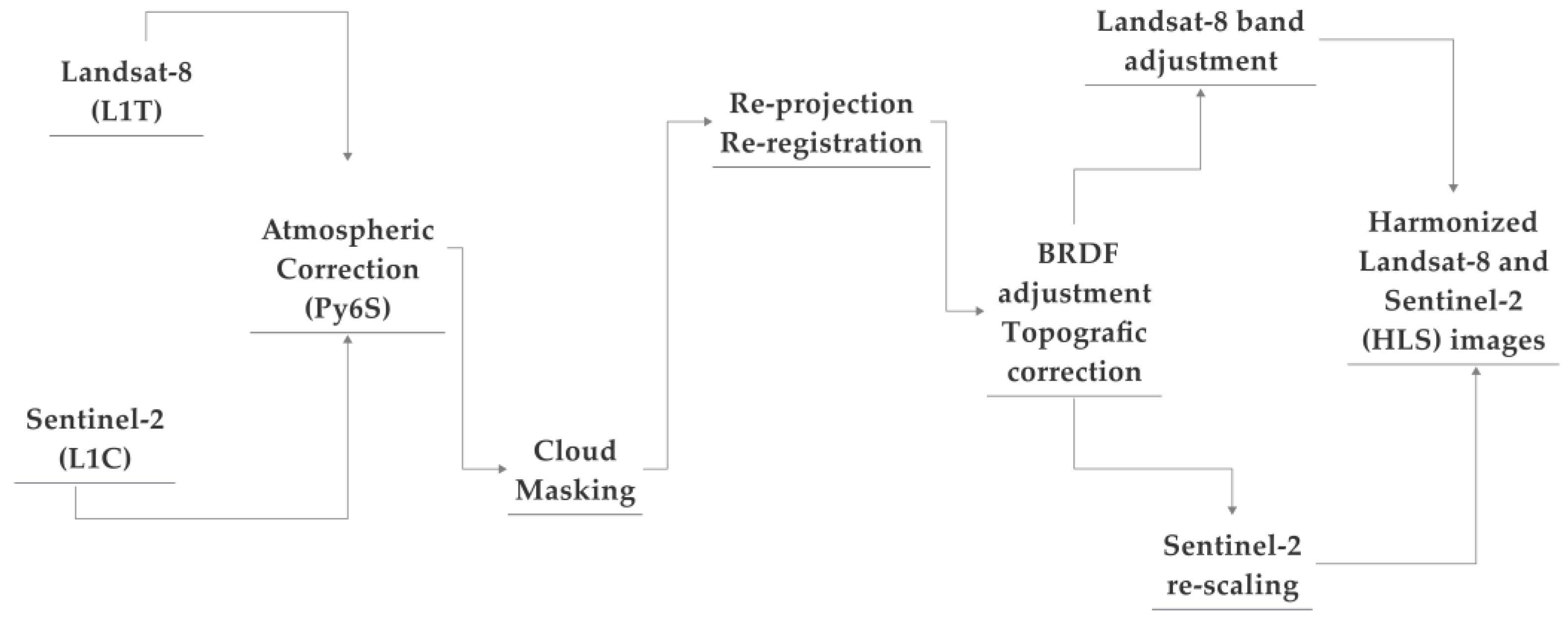
2.3. Harmonization of Landsat-8 and Sentinel-2 Data

To increment data availability, harmonization of data from different remote sensors was applied as a feasible solution to increase availability of remote sensing data and, therefore, to increase the possibilities to match up with available water quality measurements. Harmonization is a novel approach, and its implementation has been in development for general applications such as land or crop modeling. Recently, harmonization of Landsat-8 and Sentinel-2 data has been applied for water quality retrievals with promising results [14,33]. However, this process is still challenging and requires several stages of image processing [42], especially when it is intended to be used at a global scale and using entire collections of remote sensors, as in this study. For the purposes of this study, there is the need of an implementation in a cloud platform capable of processing the complete imagery of both Landsat-8 and Sentinel-2. Additionally, atmospheric correction applicable to all images is also necessary to retrieve remote sensing reflectance (Rrs). Google Earth Engine (GEE) is a cloud platform that provides excellent access to complete archives of both Landsat and Sentinel data and allows operations and corrections over the entire imagery. Currently, there are studies that describe and apply this methodology for different cases and study purposes. Particularly, we use the methodology described in [34], which is based on the original methodology by [10]. Following the above-mentioned methodology, the collections of Landsat-8 (L8) top-of-atmosphere (TOA) and Sentinel-2 (S2) Level-1C (L1C) were acquired via Google Earth Engine (GEE) for the studied lakes and dates of measurement. Images were then atmospherically corrected using the Second Simulation of the Satellite Signal in the Solar Spectrum (6S) developed by [43], which uses Radiative Transfer Models (RTMs) to simulate the passage of solar radiation across the atmosphere. The 6S algorithm was adapted to a Python (Py6S) interface [44] and implemented recently for its use with Google Earth Engine [45] via a Python API and Docker container. For cloud detection in L8 images, we applied the CFMask algorithm on GEE based on the implementation of [34]. Cloud detection in S2 images was performed with single-scene pixel-based cloud detector method developed by [46], in which cloud detection is expressed as a machine learning problem that can outperform current threshold-based cloud detection algorithms such as Fmask or Sen2Cor. This detector is already available as the s2cloudless Python package and as a tool of the sentinelhub-py library. Cloud shadow detection was conducted via the Temporal Dark Outlier Mask (TDOM) [34], which is a version adapted from [47]. TDOM applies dark pixel anomaly [48] to predict the position and the extent of a cloud’s shadows by using the cloud’s shape, height and position of the sun at that time [49]. Co-registration was performed by measuring the misalignment between L8 and S2 images (up to 38 m) [42] and aligning the L8 with its corresponding S2 [50]. Afterwards, reprojection was applied to account for possible differences in band scale and projection [51]. L8 bands from B2 through B7 were reprojected with respect to the red band of S2 (WGS84), and each band’s resolution was re-scaled to 30 m using bicubic interpolation [52,53]. The Bidirectional Reflectance Distribution Functions (BRDF) model developed by [47] was applied to reduce the directional effects due to the differences in solar and view angles between L8 and S2 [10]. This correction is based on fixed c-factors provided by [54], where the view angle is set to nadir and the illumination is set based on the center latitude of the tile [10]. The implementation of BRDF correction in GEE is based on results from different studies [54,55]. Topographic correction, which accounts for variations in reflectance due to slope, aspect and elevation, was implemented using the SRTM V3 (30 m SRTM Plus) and GTOPO30 (Global 30 ArcSecond Elevation) products to cover all Earth regions [56]. Adjustment in L8 bands was performed using cross-sensor transformation coefficients from [57] to solve spectral differences with S2 due to independent radiometric and geometric calibration processes. In [57], the absolute difference metrics and major axis linear regression analysis over 10,000 image pairs across the conterminous United States was used to obtain these transformation coefficients. The above process retrieves harmonized Landsat-8 and Sentinel-2 (HLS) images which have corrected surface reflectance with equal spectral and spatial characteristics. A detailed overview of the harmonization process is shown in Figure 2. Pixel extraction of the remote sensing reflectance (Rrs) was performed from the described location (latitude and longitude) of the field stations. We selected the main six bands from the visible, infrared and shortwave infrared, which are relevant for remote sensing of inland waters to reduce processing time.

2.4. Feature Engineering and Dataset Arrangement

Additional features were derived from the HLS dataset in search of stronger correlations. Similarly, the effect of adding additional features on the model performance was also evaluated. To this end, different types of datasets were tested. Each dataset contained different engineered features and inherent characteristics of each lake. The main differences were based on the usage of common band ratios applied to remote sensing bands [58,59,60,61,62,63,64] and additional non-radiometric features such as time and location characteristics (latitude, longitude, month and year). Data were scaled to account for better performances in the modeling process. Additional feature specifications are shown in Table 6. Four different datasets were evaluated: (i) the harmonized bands (HB) dataset contained purely the HLS bands; (ii) the feature engineering (FE) dataset contained the HLS bands plus the additional band ratios; (iii) the harmonized bands plus region and time (HBRT) dataset which contained the harmonized bands dataset in addition to time and space features, and (iv) the feature engineering plus region and time (FERT) dataset which contained the feature engineering data plus region and time. A summary of each dataset description is provided in Table 7.

2.5. Machine Learning Algorithms

Machine Learning algorithms are data-driven methods, and, therefore, they require enough in situ water quality observations that contribute to the “learning” of the model. In this process, the models establish a relationship between water leaving radiance acquired remotely [65] and the in situ observations [33]. Hence, there is an inherent empirical relationship established between target parameters and predicting features. The learning characteristic of machine learning algorithms is further evaluated in this study by considering additional predicting features that, such as the water leaving reflectance of a specific measuring point, are also intrinsic to each waterbody. This could help to improve retrievals from purely remote sensing features, which often suffer from high correlation and collinearity between them [6]. Recently applied regression models in research of remote sensing of inland waters were used as modeling approaches. Supervised learning algorithms considered were the linear regression (LR) [66,67,68,69], support vector regression (SVR) [70,71,72,73,74] and random forest (RF) [22,75,76,77]. Additionally, we employed deep learning algorithms, which have been less commonly applied in the field, from which we focused on the extreme learning machine (ELM) [13,31,78] and the multilayer perceptron regressor (MLP) [14,79,80,81].
For every target parameter, each of the above models and hyperparameter optimization with common values in GridSearch was trained and tested. Intensive hyperparameter tuning was not mainly addressed, since the primary goal was to evaluate differences in datasets for machine learning models in similar conditions. The settings of the LR model consider an intercept. Hyperparameters for SVR used a radial basis function (rbf) kernel, regularization parameter of C = 1.0 and epsilon = 0.1. We employed RFR with squared error criterion as a function to measure the quality of a split. Different activation functions were tested for ELM depending on the training data (sig, sin, radbas, hardlim, purelin and tansig), with common occurrences of sigmoidal function and hidden nodes ranging from 50–1000 for different parameters. MLP was used having five hidden layers with the ADAM activation function and a learning rate of 0.01, and Bayesian regularized backpropagation was utilized to train the model. The modeling approach was conducted using SciKit Learn (v1.0.2) in Python (v.3.10,3) and the Caret package (v2019.03.27) in R (41.3). Google CoLab was used as the cloud computing platform to perform all calculations.

2.6. Model Evaluation

Cross-validation with k = 5 folds was selected as our main method of model evaluation. The train/test split ratio was 80% training and 20% testing. Random selection of samples in each iteration was performed to ensure representative selection of data in the training and testing stages. The presence of multicollinearity in the predictors was addressed by an initial feature selection with mutual info regression as the scoring function and a second-degree polynomial feature to account for the non-linearity in the data. To ascertain model performance, we used the following quantitative error metrics: the mean absolute error (i), mean squared error (ii), root mean squared error (iii) and R2 (iv). Additionally, we considered the number of features (v) used as a metric for overall comparison among the models. It was considered that the model with the need for fewer predictors has an advantage in terms of required computing power. The error metrics were calculated for both the training and independent testing dataset. Respectively, each performance metric is defined as
R 2 y ,   y ^ = 1 i = 0 n s a m p l e s 1 y i y ^ i 2 i = 0 n s a m p l e s 1 y i y ¯ i 2
R M S E   y ,   y ^ = 1 n s a m p l e s i = 0 n s a m p l e s 1 y i y ^ i 2
M A E   y ,   y ^ = 1 i = 0 n s a m p l e s 1 y i y ^ i 2 n
where y ^ i is the estimated value, y i is the observed value and n s a m p l e s is the number of samples.

3. Results

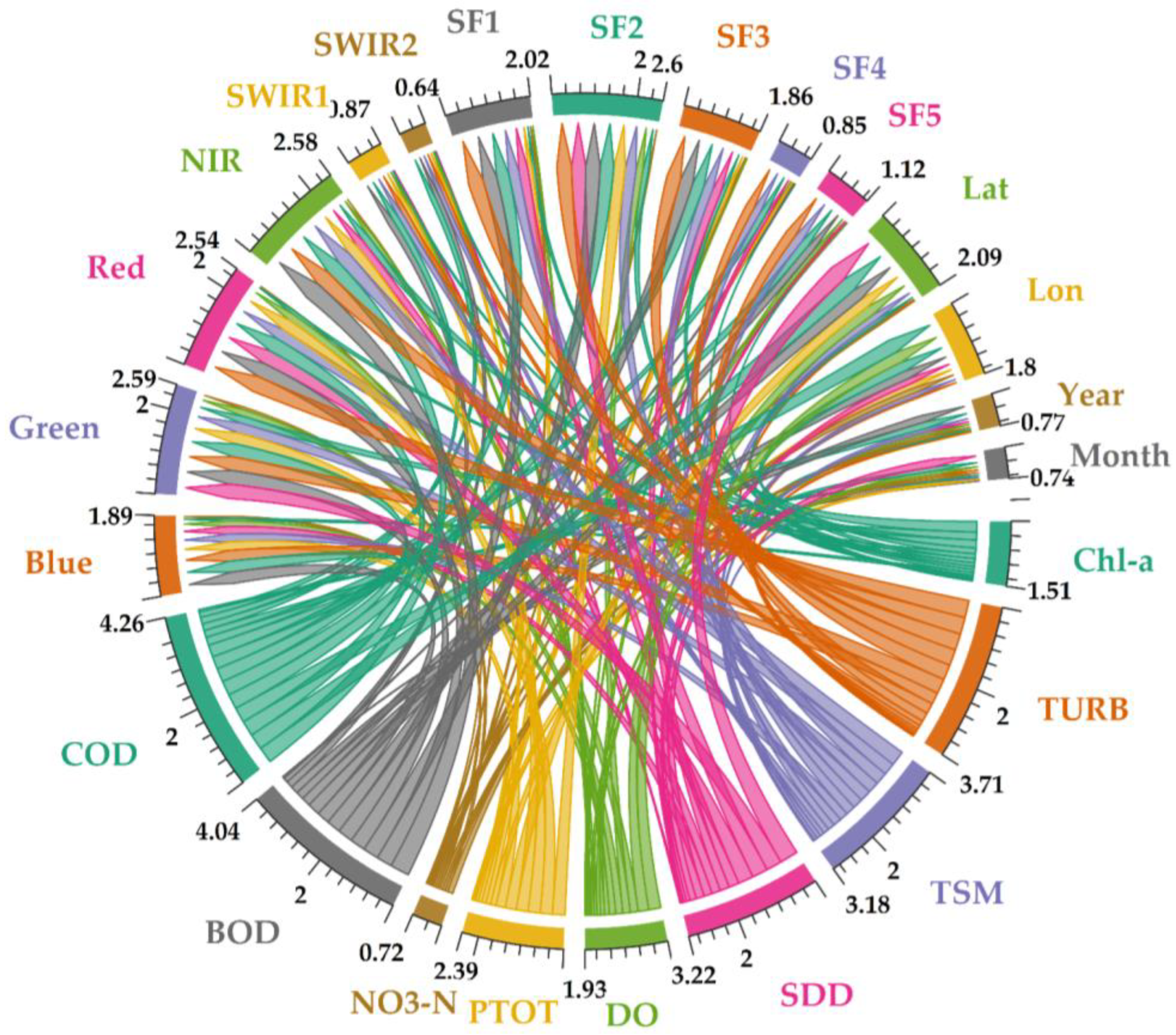
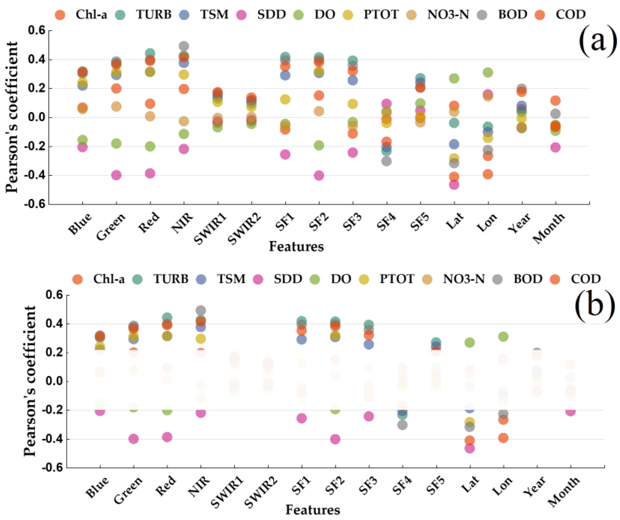
3.1. Correlation of Water Parameters and Derived Predictors

The correlation between target parameters and predicting features was investigated by the Pearson’s coefficient. The range of the coefficient for all features is shown in Figure 3. The bigger thickness in the arrow indicates a higher correlation with specific predictors. Individual plots of nodes and arrows and their correlation matrix are provided in the Supplementary Materials. Overall, the highest positive and negative correlations are in the order of r ≈ 0.50 and r ≈ −0.48. The green band is moderately correlated ( r ¯ ≈ 0.38) with turbidity, SDD, BOD and COD. The red band has a slightly higher correlation ( r ¯ ≈ 0.42) with TURB, SDD and COD. The NIR band presented the highest correlations on average (r ≈ 0.43) with TURB, TSM, BOD and COD. The SWIR bands displayed very weak correlations (0.17 ≤ r ≤ −0.07).
From the band ratios, the SF1 and SF2 had a considerable correlation with the targets. SF1 displayed ( r ¯ ≈ 0.39) with TURB, SDD, BOD and COD. SF4 and SF5 were poorly correlated (0.20 ≤ r ≤ −0.20) with all the parameters, except for an r = -0.30 and r = 0.27 for TURB. From the SF predictors, SF2 and SF3 showed a higher correlation ( r ¯ ≈ 0.39 and r ¯ ≈ 0.36) with TURB, SDD, BOD and COD. Latitude and longitude were also moderately correlated with SDD, PTOT, BOD and COD, especially latitude ( r ¯ ≈ 0.37). Year and month were poorly correlated with all analyzed predictors (0.20 ≤ r ≤ −0.20). Overall, the most correlated features were the ones of the visible and near-infrared regions, which showed higher correlation in comparison with the spectral features and the region and time features. Green, red and near-infrared bands showed higher correlations with TURB, SDD and BOD and COD. Short-wave infrared bands 1 and 2 almost completely lacked any significant correlation. Individual correlations are displayed in the supplementary figures (SF1). The NIR band and SDD parameters show the highest correlations for a predictive feature and a target parameter. Similarly, NO3-N and DO show the lower correlations for a feature and target, correspondingly.

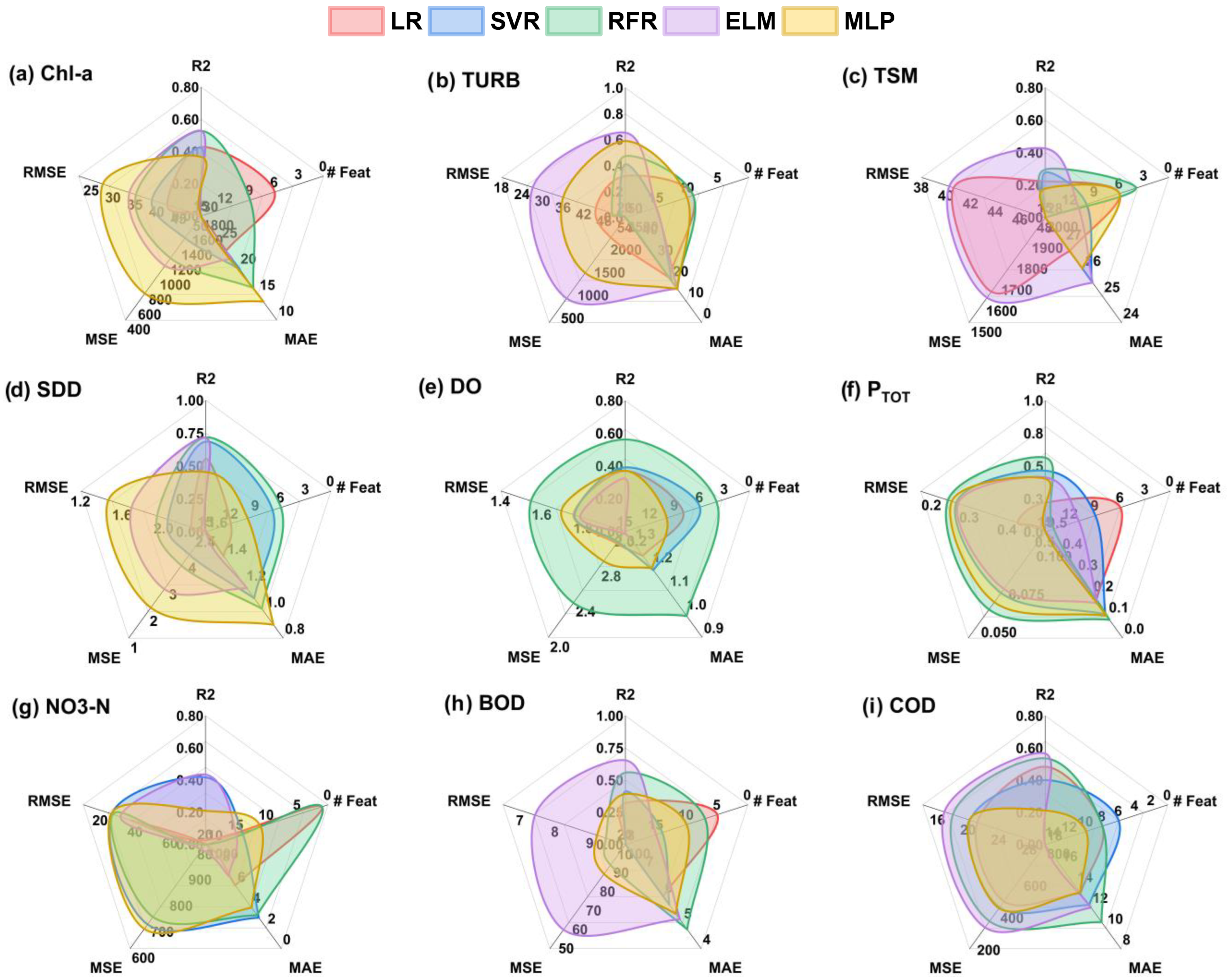
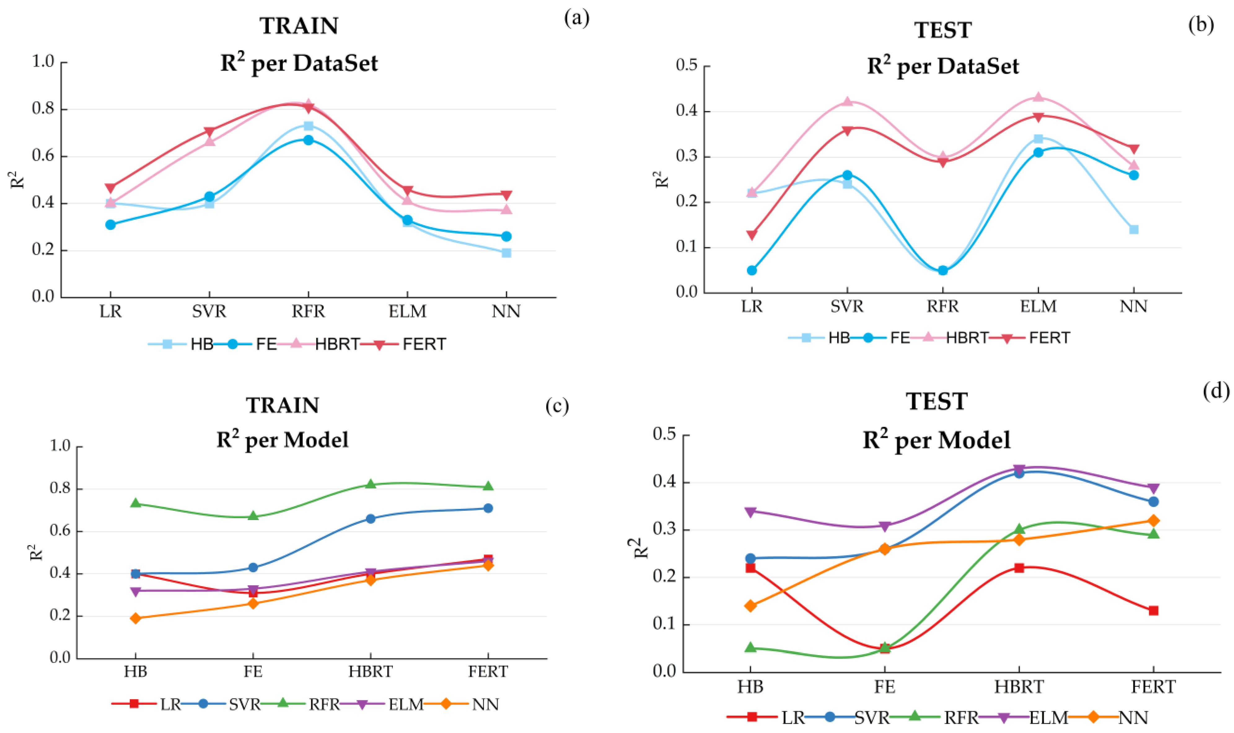
3.2. Model and Dataset Evaluation

Training and test phases were evaluated using the four available datasets (HB, FE, HBRT and FERT) for each algorithm (LR, SVR, RFR, ELM and MLP). The best dataset for each model is then shown in the table alongside the error metrics of better performance. This evaluation was performed for every target parameter. The entire modeling results are summarized in Table 8. In general, LR retrieved low-performance models ( R ¯ 2 = 0.33). It performed better on SDD and COD. However, lower performances were shown for TSS and TURB. SVR performed better than LR in most of the parameters, both for the nOACs and OACs, except for COD and Chl-a. Regarding NO3-N, most of the models performed poorly, with only SVR attaining reasonable results by retrieving R 2 = 0.42 using the HBRT dataset. In the beginning of the calibration process, RFR tended to overfit the data, even with a relatively low number of estimators in each random forest (n_estimators = 5000). This was addressed by tuning the maximum depth of each tree and the minimum number of samples required for a split.
From this routine, RFR improved greatly and retrieved most of the parameters in acceptable values mostly by using the best on HBRT, and except for NO3-N, RFR performed satisfactorily for DO ( R 2 = 0.56 ) and PTOT ( R 2 = 0.56 ). Regarding the development of the deep learning models, it was expected to establish a baseline routine of calibrated models with LR and improve it based on the SVR and RFR training methodologies to finally surpass ensemble learning models with neural networks such as ELM and MLP. Overall, ELM performed satisfactorily in most of the analyzed parameters. Specifically, ELM outperformed all algorithms when retrieving Chl-a ( R 2 = 0.53 ), TURB ( R 2 = 0.65 ), TSM ( R 2 = 0.43 ), SDD ( R 2 = 0.72 ), BOD ( R 2 = 0.65 ) and COD ( R 2 = 0.57 ). However, the results we obtained from the MLP were subpar in comparison with ELM or RFR. MLP was trained with relatively high learning rates (1 × 10⁻² to 1 × 10⁻⁵), and tests of up to 10 deep layers were used together with the Adam optimizer. Weights were initialized with random normal, as it retrieved better results than Xavier initialization. Except for TURB, MLP results generally have less accuracy than ELM and RFR.
At this point, the main metrics for model performance were R2, RMSE, MSE, MAE and the number of features utilized to reach optimal error performance in the test phase (# Feat). We compared these metrics in a comprehensive evaluation to determine the best model for each parameter. The five algorithms (LR, SVR, RFR, ELM and MLP) were trained using the best dataset determined in Table 8 to calibrate each model in its best conditions. The results of this evaluation are displayed in radial graphs in Figure 4.
In general, ELM and RFR resulted in the best models, which outperformed the rest of the machine learning techniques for most of the water parameters (Chl-a, TURB, TSM, SDD, PTOT, BOD and COD) from a comprehensive perspective. SVR performed better for the challenging NO3-N. Scatter plots of target parameters using the models calibrated with the best corresponding dataset are shown in Figure 5 for both train and test datasets. From the scatterplots it is visible that TSM, NO3-N and to a lesser degree TSM were the most challenging parameters to model and that SDD was able to be modeled with high accuracy by the ELM ( R 2 = 0.72 ), as seen in the performance in terms of error metrics in Table 8.
The results also showed that the big majority of the models for all the water parameters performed better when using any of the two datasets aware of region and time (HBRT and FERT). Therefore, a deeper analysis was performed in this direction by comparing the R2 of each dataset and the performance of each model when trained with different datasets. Figure 6 shows the average R2 for the complete modeling process, which includes not only the best results summarized in Table 8 but the rest of the models as well. Figure 6a stresses how the performances of both HBRT and FERT are superior to HB and FE for train and test evaluations. Similarly, Figure 6b shows the performance of the algorithms when using different datasets. When trained with HBRT or FERT datasets (Figure 6a, red lines; Figure 6b increased tendency from left to right), all the algorithms reached higher correlations than when trained with HB or FE (Figure 6a, blue lines; Figure 6b decreasing tendency from right to left).

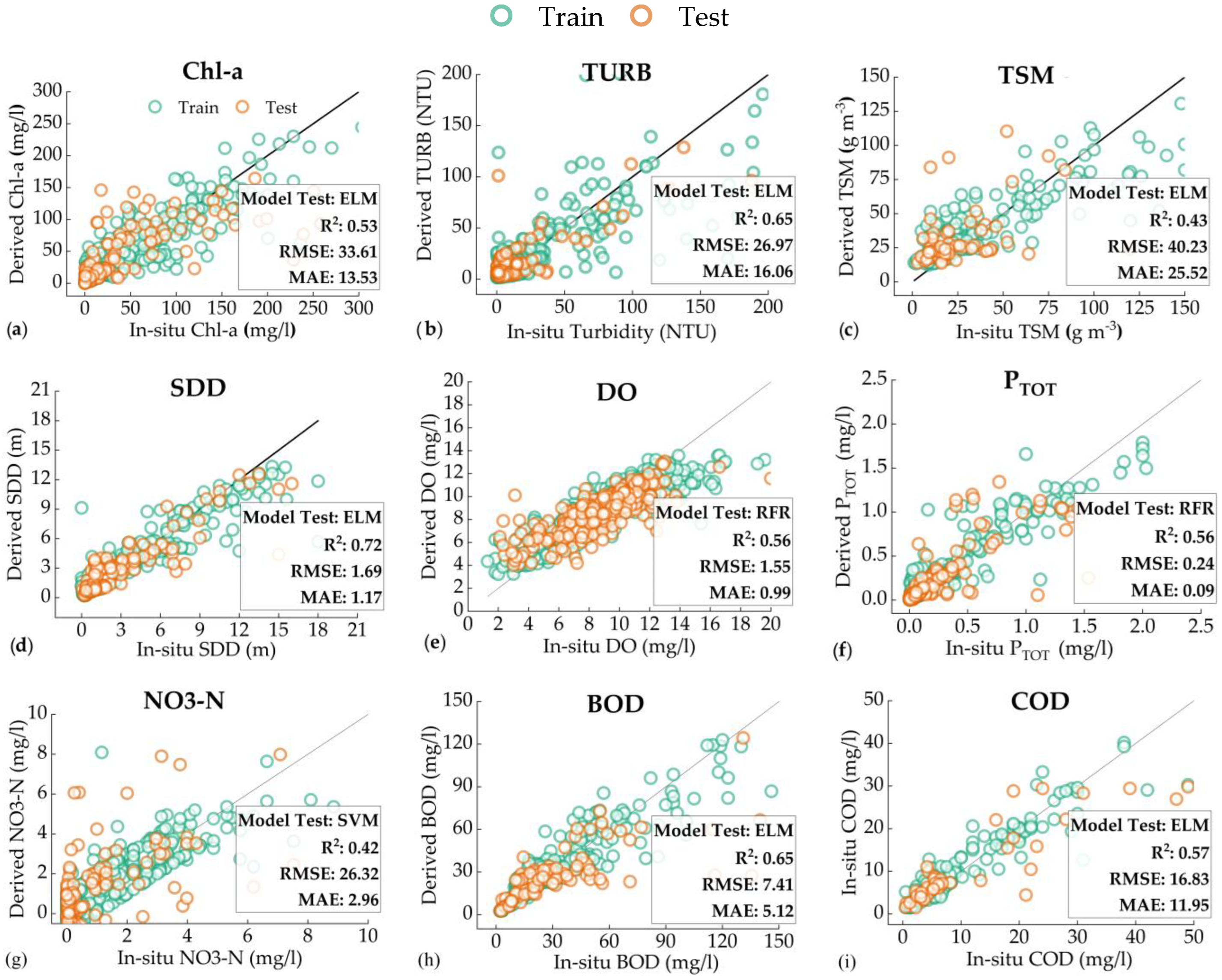
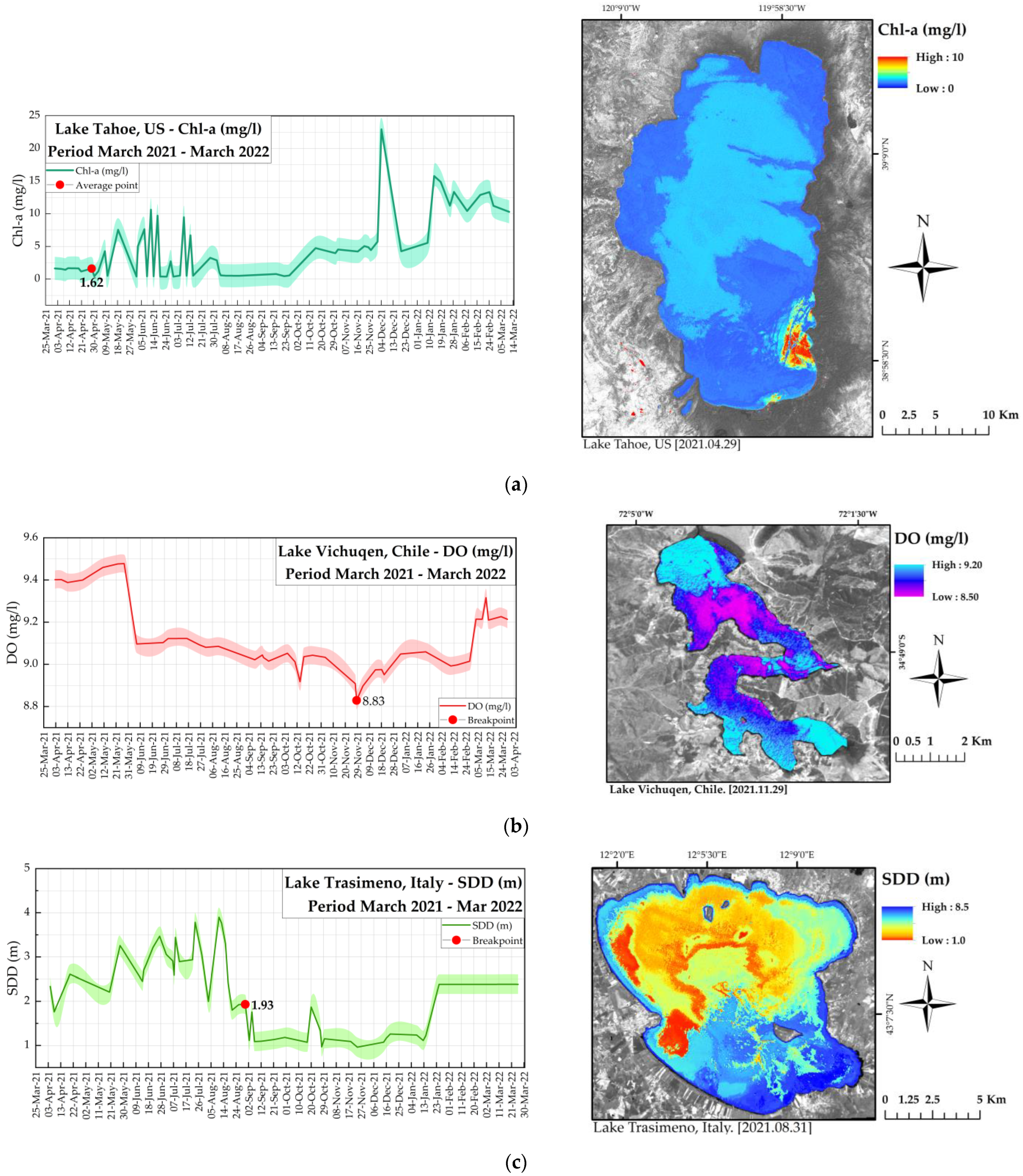
3.3. Model Capabilities

To stage model capabilities, we applied the methodology using harmonized products for the period March 2021–March 2022 to estimate time series of specific parameters (Chl-a, DO and SDD) and to model their variations throughout a year. The points marked in the evolution of the targets were used as a suitable date and to map spatial distribution. We selected different lakes around the world to test the transferability of the models. Specifically, Lake Tahoe (U.S.), Lake Trasimeno (Italy) and Lake Vichuquen (Chile) were selected for Chl-a, DO and SDD, respectively, based on field data availability. Time series and parameter maps are shown in Figure 7. Chl-a in Lake Tahoe shows concentrations between 5–10 mg/L for most of the year, but after a breaking point in December 2021, where the concentration reached its highest level above 20 mg/L, it gradually decreased and kept a range between (10–15 mg/L). DO shows low variability during the year, and it is in a range of 8.8–9.5 mg/L in Lake Vichuquen.
The lowest concentration is reached by the end of November 2021, from which it starts a recovery to higher concentrations above 9 mg/L. March, April and mid-May seem to be the months of higher availability of DO in the area. The spatial resolution of 30 m from the harmonized products allows adequate visualization of the distribution of DO even in a relatively small lake as Vichuquen (40 km2). From the map, it is visible that DO availability is higher in the outlet and inlets, located at north and south, respectively, likely caused by the turbulence and stirring of the incoming and leaving water flows. SDD in Lake Trasimeno ranges on average from 1 to 4 m during the year. The lowest transparency is seen after August 2021 (≈1 m) and remains in this range until its recovery in January 2022 of 2.5 m. The breaking point in August is selected as the date of interest for a spatial visualization (31 August 2021). The surface distribution of SDD reveals a big cluster of lower transparency in the northwest part of the lake. The south part, which is an open bay, remains clearer.

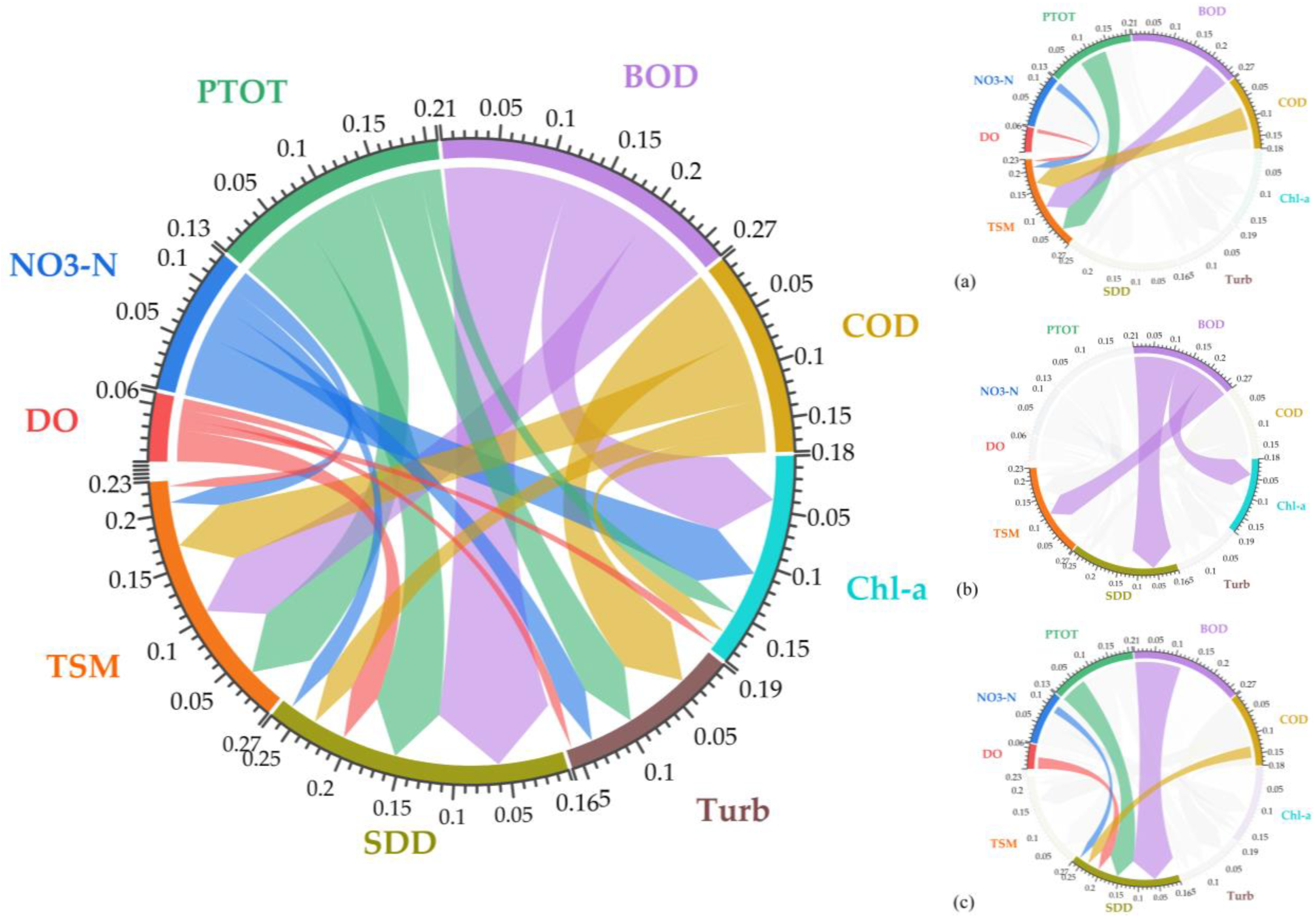
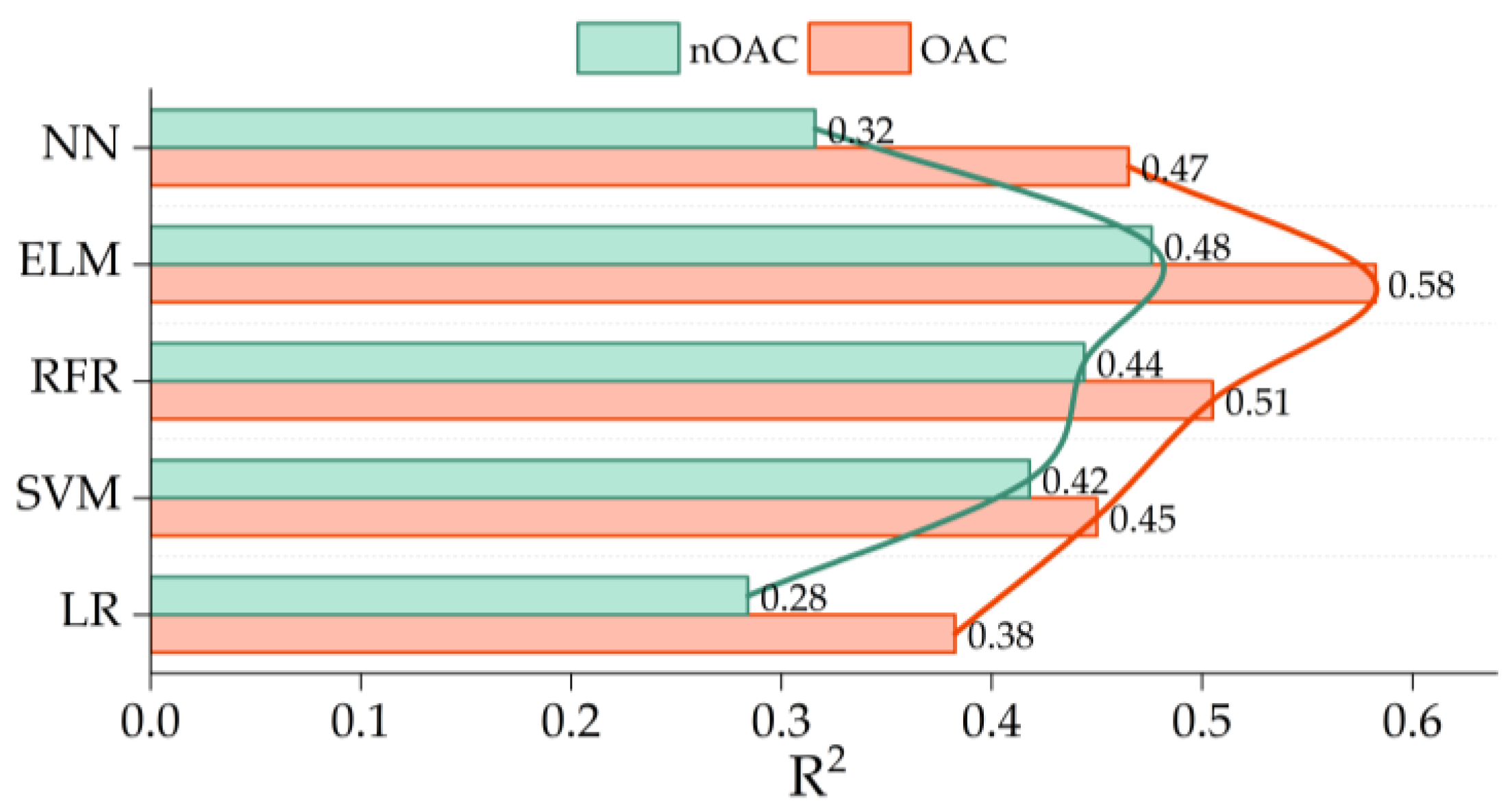
3.4. Correlation between OAC and nOAC

For the specific case of nOACs (DO, NO3-N, PTOT, BOD and COD), their estimation resulted in a challenging approach, as seen in the results of Table 8 and Figure 4 and Figure 5. For NO3-N only SVR was able to produce reasonable results (R2 = 0.42). To further evaluate the possibility of estimating nOAC using indirect means, a correlation analysis between OAC and nOAC was performed and is displayed in Figure 8. Similar to Figure 3, each node of the Chor diagram shows the sum of absolute values of Pearson’s correlation. Separate individual nodes are available in the Supplementary Materials. From the results, no significant correlations between OAC and nOAC were retrieved, as seen in the total absolute value of the nodes in Figure 8, which barely overpass r ¯ ≈ 0.20 for TSM (Figure 8a), BOD (Figure 8b) and SDD (Figure 8c). These results stress the difficulty of estimating nOAC from indirect methods which could rely on relevant correlations with OAC that can be computed via remote sensing.

4. Discussion

4.1. Global Water Quality Data Availability

The availability of water quality data at a global scale that can be used in synergy with remote sensing data is still very limited. In this study, the raw gathered data were filtered substantially and went from initial 300,000 measurements of all the parameters around the globe to a final dataset of around 7000 samples after data selection. This is still an important amount of data in comparison with the available data in previous years or other studies of water quality in inland waters [12,31,75,82,83]. Regarding the sampling sites and depths in the considered waterbodies, this study considered the location of the sites during the cleaning phase of the data and rejected samples that were adjacent to the shore to avoid the adjacency error. This is a similar approach to a previous study that successfully utilized a wide range of sampling sites in [31]. Although this work focused on the water column and avoided shallow regions close to the coast and bottom of the reservoir, rejection of lakes or reservoirs based on average depth was not performed. Here, it is acknowledged that a more targeted approach to sampling could improve the quality of the results and suggested that future studies consider the location and depth of the sampling sites to minimize potential errors.
However, it cannot be denied that the water availability at a global level is limited by several factors that can be improved based on the inter-cooperation of different instances and technical issues. For example, measuring stations at the global level are limited to certain areas around the world. In this work, we notice a lack of water information for large parts of the planet, particularly in South America, Africa and Asia. As exposed in Section 2, the study of Thorslund and van Vliet [35] indicates that most of the measuring water stations for lakes and reservoirs were located in North America (with big differences) and Europe. This exposes how a very important number of inland waters are not being monitored. Additionally, the integration of global data is constrained by the fact that every nation is responsible for the technical requirements of water monitoring and making data public. Therefore, it is likely that already monitored data from several regions in the world are not yet available to a greater extent due to limitations in this direction, and therefore their usage may be missed for global applications. In worse cases, gathering global data could even be limited by trifling facts as ignorance of foreign languages. Thus, international cooperation is then needed to apply team-work to data availability. In this sense, initiatives such as the Global Freshwater Quality Database (GEMStat) from the UN Environmental Program [1] offer an adequate framework for the previously mentioned challenges.

4.2. Harmonized Remote Sensing Data for Water Quality Estimation

In addition to field data availability, remote sensing also has important limitations in modeling full potential water quality at the global scale. For instance, temporal resolution limits the coupling of spectral and field data. In this study, we addressed this limitation up to a certain degree by harmonizing Landsat-8 and Sentinel-2 data, which increased data availability. This allowed the use of coupled satellite data in a singular dataset, which was one the main objectives of this study.
However, the current harmonization process is not specifically designed for inland waters. Similarly, the atmospheric correction used in [34], the Second Simulation of the Satellite Signal in the Solar Spectrum (6S), is also not designed for waterbodies, as it occurs with other corrections designed for inland waters such as C2RCC. Therefore, the results based on this methodology should be taken with caution, since discrepancies from a harmonization process and an atmospheric correction for different applications than water quality retrievals are likely to exist. The main reason this study applied these methodologies was the existing implementation in the cloud platform used for image processing. There is no current harmonization process or atmospheric correction developed for cloud computing in GEE that is designed to enhance the spectral characteristics of water surfaces, and working with the entire collection of Landsat and Sentinel satellites was not feasible using local computational resources. Developing both a harmonization procedure and an atmospheric correction for the cloud platform was out of the objectives of this research. However, the harmonization procedure is still in development, and it is likely to account for water surface characteristics in the future [84]. Likewise, the 6S atmospheric correction is a common procedure in remote sensing and it has already been implemented in mapping and water quality monitoring [85]. Adopting the above-described methodology allowed the building of a global dataset for model development and contributed to understanding to what extent machine learning can benefit from increased data availability.
Nevertheless, non-coupled satellite acquisitions and dates of water measurements were two of the main filters that avoided the usage of a great portion of the gathered data. The spatial resolution also constrains availability when the resolution is not enough to retrieve enough pixels from very small reservoirs. The pixel size of harmonized data is 30 × 30 m, which allows consideration of a big number of lakes and reservoirs. However, it may not be the best resolution for inland waters below surfaces of 20 km2 due to possible errors caused by bottom reflection and adjacency errors caused by land next to shores. Therefore, the revisit time of harmonized data (3 days), even when it may be considered adequate in the field, is probably not good enough to monitor changes in water parameters that could exhibit great variations even during one single day and to account for a great part of the available field data, as seen in this study. Therefore, the tendency to improve temporal and spatial resolutions is highly important, as some ground-based high-frequency sensors already demonstrate [86].

4.3. Machine Learning Models and Cloud Computing

ML models provide research in water quality the possibility to model and estimate different water parameters with a high degree of accuracy based on adequate data availability [21,87,88]. In addition, the variety and distinct nature of available ML algorithms for modeling purposes foster rigorous evaluation of the methodology and contribute to reaching stronger and more developed models [14,33]. In this study, we focused on the “learning” advantage of ML models and tried to provide as much data as possible by means of global measurements and remote sensing data fusion techniques, with the goal of reaching robust models that could retrieve water quality parameters accurately. As in previous research using ML approaches, we could develop models that predict water quality parameters with reasonable results. Furthermore, a key improvement in the direction of modeling at the global scale was achieved, which has been one of the main limitations of modeling water quality of inland waters [6,7] and that was only addressed before by bio-optical models with more complex approaches in terms of development [7,33,89]. The extent of the regionalization modeling is precisely the advantage that ML models offer when providing enough and high-quality data. In this study, we showed how the contribution of enough high-quality input data and adequate calibration of ML models could start pushing existing research barriers. In this sense, the potential for improvement of the ML models is still enormous, particularly with the progressive increment in data availability coming from more frequent field campaigns, better acquisition sensors and disclosure of non-public data. Therefore, modeling global water quality in inland waters should be considered as a continuous area of research and development with the goal to achieve models that improve continuously from constant monitoring. In addition to the above-mentioned limitations, challenges regarding computational power and storage space existed. The large number of models to be tested plus even small calibration techniques resulted in extensive computing periods which could not be covered by our locally available hardware resources. Therefore, a cloud computing platform (Google Colab) was required to address this problem and proceed with model evaluation. Cloud computing allows parallel computing while focusing cloud servers only for computational tasks. This methodology distributes more efficiently available resources and should be considered for similar tasks, especially when dealing with large datasets. Similarly, the usage of Google Earth Engine also allowed working efficiently with the vast quantity of remote sensing data products of the match ups with field measurements, and thanks to previous knowledge of state-of-the-art applications on the harmonizing process [10,14,34,47,54], these limitations were diminished.
The potential for global monitoring was already addressed by [90] with a synthetic dataset of top-of-atmosphere and bottom-of-atmosphere reflectances to comprise optical variability present in inland waters. Regarding field data measured on Earth, and to the extent of the authors’ knowledge, this is the first attempt to model water quality on a global scale using remote sensing data based on machine learning algorithms. Therefore, the comparison of the models developed here is complicated because, until the submission of this paper, there are no similar studies that attempt similar modeling scales. However, based on the well-established validation methodology applied, the reasonable performance of the models and its adequate application in time series and water quality maps, we posit that our methodology is on the way to establishing a basis for future development in this research area. With the distances apart and for an exercise of comparison, the results here yielded were compared with novel publications that have successfully developed ML models for inland water quality. For example, error metrics of Chl-a (R2 = 0.53), TURB (R2 = 0.65) and DO R2 = 0.56) from ELM and RFR are comparable with modeling results observed in [33] of Chl-a (R2 = 0.48), TURB (R2 = 0.44) and DO R2 = 0.21. On the other hand, PTOT (R2 = 0.56), NO3-N (R2 = 0.42), BOD (R2 = 0.65) and COD (R2 = 0.57) are comparable with the results of Zhang et al. [88] regarding phosphorus (R2 = 0.94), nitrogen (R2 = 0.95), BOD (R2 = 0.91) and COD (R2 = 0.95), which were retrieved from hyperspectral images. Regarding the poor performance of the MLP, the strategy was to build neural nets deep and wide enough to first overfit the data and then reduce them. However, this operation could not be totally completed due to a lack of dedicated GPUs (even in the cloud server) and time constraints. Even in the best performing parameter (TURB), most of the MLP results were in the underfitting range, and train and test splits showed similar error metrics. These results may provide a clear picture of the behavior of a partially optimized MLP.

4.4. Estimation of OAC and nOAC

The estimation of OAC with remote sensing has been addressed extensively in research for least two decades [12,19,22,60,82,91,92,93,94,95,96,97,98,99]. Particularly, parameters such as SDD, turbidity or Chl-a and TSM have been studied with great detail, and their estimation has been the target of different modeling approaches, from empirical to semi-analytical models [26,83,95,100,101,102,103,104,105,106,107,108,109,110]. nOAC, however, represented a greater challenge because of its lack of response to absorption or scattering of the electromagnetic light [7].
A direct estimation of nOAC from RS data has been previously investigated. For example, [73] used SVM and SPOT5 data for potassium permanganate index (CODmn), ammonia nitrogen (NH3-N), chemical oxygen demand (COD) and dissolved oxygen (DO) in the Weihe River with better performance than the statistical regression. Recently, [111] used ML models for spatial distributions of the annual and monthly DO variability in Lake Huron from Landsat and MODIS data with consistent values of R2 = 0.88. Similarly, [88] used a Bayesian probabilistic neural network to predict phosphorus, nitrogen, chemical oxygen demand (COD), biochemical oxygen demand (BOD) and chlorophyll-a from hyperspectral images in a river from multispectral images. We compared the average R2 summary of the OAC (Chl-a, TURB, TSM and SDD) and nOAC (DO, PTOT, NO3-N, BOD and COD) to contrast how the results also show that in general nOAC presents more challenges than OAC (Figure 9). All the models achieved higher results in OAC, but at the same time nOAC results were reasonable and did not show an incapacity to model these parameters. This reinforces the fact that ML models are also suited to deal with parameters with non-linear relationships between remote sensing data or inherent lake characteristics, contributing to the improvement of modeling nOAC.

4.5. Inherent Lakes’ Characteristics as Model Improvers

Typically, semi-empirical models in the field of remote sensing of inland waters do rely on the physics knowledge of the optics in the water and the response of water or water constituents to the interaction with the electromagnetic energy. One main objective of this study was to evaluate this conventional approach against more unconventional methodology that could rely more on the learning capability of the ML algorithms. On the basis that these algorithms work better with a higher number of observations and adequate predictors that explain better the behavior of the targets, we selected additional characteristics of each lake to evaluate possible improvements in comparison with purely radiometric remote sensing bands or band ratios already tested in the previous literature. The cautious evaluation of the impact on model performance is that the addition of these characteristics would have led to the creation of four different datasets: HB, FE, HBRT and FERT. Region and time were the selected characteristics added to the original datasets, the product of the remote sensing data. The correlation analysis revealed a moderate correlation with the water parameters for latitude and longitude and very weak correlations for year and month. Figure 10 stresses this situation.
In Figure 10a it is seen how the visible bands and band ratios show a higher correlation. SWIR bands and year and month are in a very weak range, as displayed in Figure 10b, where the region −0.20 ≤ r ≤ 0.20 is covered to highlight stronger correlations. The occurrence that Lat and Lon are having a stronger correlation than year and month means, therefore, that a greater utility in model development could be due to the fact that year and month are not strictly inherent characteristics of a waterbody. Their inclusion was mainly because of the fact that the time and seasonality have important influences on the behavior of certain water quality, such as the blooming of algae or the arrival of storms that discharge waters with sediment, creating turbidity. Nevertheless, the improvement in error metrics of all the water parameters when ML models used HB and FERT datasets was evident and validated in our methodology (Figure 11). This leads us to the conclusion that this approach resulted in an effective improvement of the modeling of water quality parameters by the addition of inherent lake characteristics that can be useful for ML algorithms.
Therefore, research in this direction is needed to keep the improvement of the modeling process and to develop more accurate models. There are several inherent characteristics that may be useful for such purposes and that can be found in constant patterns in time, such as trophic state and chemical, biological, physical, limnological or morphological features. Time features can be improved or added as labels for the season of the year, as seen in [111].

5. Conclusions

This work developed machine learning models for water quality retrieval at a global scale using remote homogenized multimodal remote sensing data. This contributed to overcoming the present state of knowledge in which the transferability of models is limited by the origin of field data, and modeling water quality in inland waters at different locations was constrained. These findings directly impact the increment of our ability to analyze lakes and reservoirs globally, particularly for several water parameters of different nature and characteristics, which are key in the overall understanding of water quality in lakes and reservoirs. This work is limited by the amount and origin of the field data gathered and the extent of the remote sensing archives processed. The application of the models developed here was demonstrated at the global scale in different lakes separated by continental distances. However, the usage of these models in regions from where there were no data in the calibration process is likely to be poorly accurate and would lack reliability in results. Therefore, the methodology should be improved by gathering data from more and different sources around the world, particularly from the African, Asian and South American continents. Remote sensing data can be increased by harmonizing data from older satellites, such as the Landsat constellation, and extending the current dataset. Thus, future work should focus on increasing the data availability of both remote sensing and global data in the field and incorporating the advances in remote sensing research such as correction of adjacency errors and improvement of atmospheric correction.

Supplementary Materials

The following supporting information can be downloaded at: https://www.mdpi.com/article/10.3390/rs15051390/s1, Figures: SF1 vidual sum of correlations of each predictor and target in form of Chord diagram.

Author Contributions

L.F.A.-R. conceived this study. U.F.T. conducted main data processing and analysis of the harmonized RS data. U.F.T. and L.F.A.-R. conducted data processing and modeling analysis. L.F.A.-R. wrote the original version of the manuscript. Constructive comments and improvements of the manuscript were provided by Z.D., J.H., Y.T. and M.D. through extensive discussion. All authors have read and agreed to the published version of the manuscript.

Funding

This article was accomplished with the financial support for research of the Mexican National Council for Science and Technology (CONACYT) and the Federal Department of Energy (SENER) through its funding “CONACYT-SENER Sustentabilidad Energética” CVU 678957. In addition, this work was supported by the German Research Foundation (DFG) and the Technical University of Munich (TUM) in the framework of the Open-Access Publishing Program.

Acknowledgments

The authors thank all the national and international agencies and the personnel involved in the acquisition of field water quality data around the world. They would also like to thank the Technical University of Munich (TUM) and its Graduate School (TUM-GS) for the institutional services and facilities necessary to perform this study. The authors also thank the ESA, NASA and USGS agencies for providing the necessary radiometric data and software to process these data. Additionally, they acknowledge Marco Körner from the TUM Chair of Remote Sensing Technology for valuable discussions about the methodology.

Conflicts of Interest

The authors declare no conflict of interest.

References

  1. UNEP. A Snapshot of the World’s Water Quality: Towards a Global Assessment; United Nations Environment Programme: Nairobi, Kenya, 2016; p. 162. [Google Scholar]
  2. UNEP. GEMStat 2020. Website Data Portal. Available online: https://gemstat.bafg.de/applications/public.html?publicuser=PublicUser#gemstat/Stations (accessed on 15 February 2021).
  3. Anon. An Integrated Water-Monitoring Network for Wisconsin; G.S.U. Water Resources Center, Ed.; University of Wisconsin: Madison, WI, USA, 1998. [Google Scholar]
  4. EPA. Elements of a State Water Monitoring and Assessment Program; Environmental Protection Agency, Assessment and Watershed Protection Division, Office of Wetlands, Oceans and Watershed: Washington, DC, USA, 2001.
  5. Gholizadeh, M.H.; Melesse, A.M.; Reddi, L. A Comprehensive Review on Water Quality Parameters Estimation Using Remote Sensing Techniques. Sensors 2016, 16, 1298. [Google Scholar] [CrossRef] [Green Version]
  6. Matthews, M.W. A current review of empirical procedures of remote sensing in inland and near-coastal transitional waters. Int. J. Remote Sens. 2011, 32, 6855–6899. [Google Scholar] [CrossRef]
  7. Giardino, C.; Brando, V.E.; Gege, P.; Pinnel, N.; Hochberg, E.; Knaeps, E.; Reusen, I.; Doerffer, R.; Bresciani, M.; Braga, F.; et al. Imaging Spectrometry of Inland and Coastal Waters: State of the Art, Achievements and Perspectives. Surv. Geophys. 2019, 40, 401–429. [Google Scholar] [CrossRef] [Green Version]
  8. Doxaran, D.; Froidefond, J.M.; Lavender, S.; Castaing, P. Spectral signature of highly turbid waters: Application with SPOT data to quantify suspended particulate matter concentrations. Remote Sens. Environ. 2002, 81, 149–161. [Google Scholar] [CrossRef]
  9. IOCCG. Remote Sensing of Ocean Colour in Coastal, and Other Optically-Complex. In Waters; Sathyendranath, S., Ed.; IOCCG: Dartmouth, NS, Canada, 2000. [Google Scholar]
  10. Claverie, M.; Ju, J.; Masek, J.G.; Dungan, J.L.; Vermote, E.F.; Roger, J.-C.; Skakun, S.V.; Justice, C. The Harmonized Landsat and Sentinel-2 surface reflectance data set. Remote Sens. Environ. 2018, 219, 145–161. [Google Scholar] [CrossRef]
  11. Zhang, Y.; Ma, R.; Duan, H.; Loiselle, S.; Xu, J. A Spectral Decomposition Algorithm for Estimating Chlorophyll-a Concentrations in Lake Taihu, China. Remote Sens. 2014, 6, 5090–5106. [Google Scholar] [CrossRef] [Green Version]
  12. Bonansea, M.; Rodriguez, M.C.; Pinotti, L.; Ferrero, S. Using multi-temporal Landsat imagery and linear mixed models for assessing water quality parameters in Río Tercero reservoir (Argentina). Remote Sens. Environ. 2015, 158, 28–41. [Google Scholar] [CrossRef]
  13. Peterson, K.T.; Sagan, V.; Sidike, P.; Cox, A.L.; Martinez, M. Suspended Sediment Concentration Estimation from Landsat Imagery along the Lower Missouri and Middle Mississippi Rivers Using an Extreme Learning Machine. Remote Sens. 2018, 10, 1503. [Google Scholar] [CrossRef] [Green Version]
  14. Peterson, K.T.; Sagan, V.; Sloan, J.J. Deep learning-based water quality estimation and anomaly detection using Landsat-8/Sentinel-2 virtual constellation and cloud computing. GISci. Remote Sens. 2020, 57, 510–525. [Google Scholar] [CrossRef]
  15. Pyo, J.; Cho, K.H.; Kim, K.; Baek, S.-S.; Nam, G.; Park, S. Cyanobacteria cell prediction using interpretable deep learning model with observed, numerical, and sensing data assemblage. Water Res. 2021, 203, 117483. [Google Scholar] [CrossRef]
  16. He, J.; Chen, Y.; Wu, J.; Stow, D.A.; Christakos, G. Space-time chlorophyll-a retrieval in optically complex waters that accounts for remote sensing and modeling uncertainties and improves remote estimation accuracy. Water Res. 2020, 171, 115403. [Google Scholar] [CrossRef]
  17. Chen, K.; Chen, H.; Zhou, C.; Huang, Y.; Qi, X.; Shen, R.; Liu, F.; Zuo, M.; Zou, X.; Wang, J.; et al. Comparative analysis of surface water quality prediction performance and identification of key water parameters using different machine learning models based on big data. Water Res. 2020, 171, 115454. [Google Scholar] [CrossRef]
  18. Chen, Y.; Arnold, W.A.; Griffin, C.G.; Olmanson, L.G.; Brezonik, P.L.; Hozalski, R.M. Assessment of the chlorine demand and disinfection byproduct formation potential of surface waters via satellite remote sensing. Water Res. 2019, 165, 115001. [Google Scholar] [CrossRef] [PubMed]
  19. Li, Y.; Wang, X.; Zhao, Z.; Han, S.; Liu, Z. Lagoon water quality monitoring based on digital image analysis and machine learning estimators. Water Res. 2020, 172, 115471. [Google Scholar] [CrossRef] [PubMed]
  20. Xu, T.; Coco, G.; Neale, M. A predictive model of recreational water quality based on adaptive synthetic sampling algorithms and machine learning. Water Res. 2020, 177, 115788. [Google Scholar] [CrossRef]
  21. Zhang, Y.; Wu, L.; Deng, L.; Ouyang, B. Retrieval of water quality parameters from hyperspectral images using a hybrid feedback deep factorization machine model. Water Res. 2021, 204, 117618. [Google Scholar] [CrossRef] [PubMed]
  22. Arias-Rodriguez, L.F.; Duan, Z.; Sepúlveda, R.; Martinez-Martinez, S.I.; Disse, M. Monitoring Water Quality of Valle de Bravo Reservoir, Mexico, Using Entire Lifespan of MERIS Data and Machine Learning Approaches. Remote Sens. 2020, 12, 1586. [Google Scholar] [CrossRef]
  23. Hartling, S.; Sagan, V.; Sidike, P.; Maimaitijiang, M.; Carron, J. Urban tree species classification using a WorldView-2/3 and LiDAR data fusion approach and deep learning. Sensors 2019, 19, 1284. [Google Scholar] [CrossRef] [PubMed] [Green Version]
  24. Sidike, P.; Sagan, V.; Maimaitijiang, M.; Maimaitiyiming, M.; Shakoor, N.; Burken, J.; Mockler, T.; Fritschi, F.B. dPEN: Deep Progressively Expanded Network for mapping heterogeneous agricultural landscape using WorldView-3 satellite imagery. Remote Sens. Environ. 2019, 221, 756–772. [Google Scholar] [CrossRef]
  25. Maimaitijiang, M.; Sagan, V.; Sidike, P.; Hartling, S.; Esposito, F.; Fritschi, F.B. Soybean yield prediction from UAV using multimodal data fusion and deep learning. Remote Sens. Environ. 2020, 237, 111599. [Google Scholar] [CrossRef]
  26. Pahlevan, N.; Smith, B.; Schalles, J.; Binding, C.; Cao, Z.; Ma, R.; Alikas, K.; Kangro, K.; Gurlin, D.; Nguyen, H.; et al. Seamless retrievals of chlorophyll-a from Sentinel-2 (MSI) and Sentinel-3 (OLCI) in inland and coastal waters: A machine-learning approach. Remote Sens. Environ. 2020, 240, 111604. [Google Scholar] [CrossRef]
  27. Zhang, L.; Zhang, L.; Du, B. Deep learning for remote sensing data: A technical tutorial on the state of the art. IEEE Geosci. Remote Sens. Mag. 2016, 4, 22–40. [Google Scholar] [CrossRef]
  28. Ball, J.E.; Anderson, D.T.; Chan Sr, C.S. Comprehensive survey of deep learning in remote sensing: Theories, tools, and challenges for the community. J. Appl. Remote Sens. 2017, 11, 042609. [Google Scholar] [CrossRef] [Green Version]
  29. Alom, M.Z.; Taha, T.M.; Yakopcic, C.; Westberg, S.; Sidike, P.; Nasrin, M.S.; Hasan, M.; Van Essen, B.C.; Awwal, A.A.S.; Asari, V.K. A State-of-the-Art Survey on Deep Learning Theory and Architectures. Electronics 2019, 8, 292. [Google Scholar] [CrossRef] [Green Version]
  30. Ma, L.; Liu, Y.; Zhang, X.; Ye, Y.; Yin, G.; Johnson, B.A. Deep learning in remote sensing applications: A meta-analysis and review. ISPRS J. Photogramm. Remote Sens. 2019, 152, 166–177. [Google Scholar] [CrossRef]
  31. Arias-Rodriguez, L.F.; Duan, Z.; de Jesús Díaz-Torres, J.; Basilio Hazas, M.; Huang, J.; Kumar, B.U.; Tuo, Y.; Disse, M. Integration of Remote Sensing and Mexican Water Quality Monitoring System Using an Extreme Learning Machine. Sensors 2021, 21, 4118. [Google Scholar] [CrossRef]
  32. Szegedy, C.; Liu, W.; Jia, Y.; Sermanet, P.; Reed, S.; Anguelov, D.; Erhan, D.; Vanhoucke, V.; Rabinovich, A. Going deeper with convolutions. In Proceedings of the IEEE Conference on Computer Vision and Pattern Recognition, Boston, MA, USA, 7–12 June 2015; pp. 1–9. [Google Scholar]
  33. Sagan, V.; Peterson, K.T.; Maimaitijiang, M.; Sidike, P.; Sloan, J.; Greeling, B.A.; Maalouf, S.; Adams, C. Monitoring inland water quality using remote sensing: Potential and limitations of spectral indices, bio-optical simulations, machine learning, and cloud computing. Earth-Sci. Rev. 2020, 205, 103187. [Google Scholar] [CrossRef]
  34. Nguyen, M.; Baez-Villanueva, O.; Bui, D.; Nguyen, P.; Ribbe, L. Harmonization of Landsat and Sentinel 2 for Crop Monitoring in Drought Prone Areas: Case Studies of Ninh Thuan (Vietnam) and Bekaa (Lebanon). Remote Sens. 2020, 12, 281. [Google Scholar] [CrossRef] [Green Version]
  35. Thorslund, J.; van Vliet, M.T. A global dataset of surface water and groundwater salinity measurements from 1980–2019. Sci. Data 2020, 7, 1–11. [Google Scholar] [CrossRef] [PubMed]
  36. WQP. Water Quality Portal. 2021. Available online: https://www.waterqualitydata.us/wqp_description/ (accessed on 15 January 2022).
  37. GobMX. Calidad del agua en México. 2021. Available online: https://www.gob.mx/conagua/articulos/calidad-del-agua (accessed on 15 January 2022).
  38. GobCa. Open Government Portal. 2021. Available online: https://search.open.canada.ca/en/od/ (accessed on 15 January 2022).
  39. GobChl. Ministerio de Obras Públicas, MOP—Morandé 59, Santiago de Chile. Direccion General de Aguas. Available online: https://dga.mop.gob.cl/servicioshidrometeorologicos/Paginas/default.aspx (accessed on 15 January 2022).
  40. Bulgarelli, B.; Kiselev, V.; Zibordi, G. Adjacency effects in satellite radiometric products from coastal waters: A theoretical analysis for the northern Adriatic Sea. Appl. Opt. 2017, 53, 1523–1545. [Google Scholar] [CrossRef] [PubMed]
  41. Lehner, B.; Döll, P. Development and validation of a global database of lakes, reservoirs and wetlands. J. Hydrol. 2004, 296, 1–22. [Google Scholar] [CrossRef]
  42. Storey, J.; Roy, D.P.; Masek, J.; Gascon, F.; Dwyer, J.; Choate, M. A note on the temporary misregistration of Landsat-8 Operational Land Imager (OLI) and Sentinel-2 Multi Spectral Instrument (MSI) imagery. Remote Sens. Environ. 2016, 186, 121–122. [Google Scholar] [CrossRef] [Green Version]
  43. Vermote, E.F.; Tanré, D.; Deuze, J.L.; Herman, M.; Morcette, J.-J. Second Simulation of the Satellite Signal in the Solar Spectrum, 6S: An overview. IEEE Trans. Geosci. Remote Sens. 1997, 35, 675–686. [Google Scholar] [CrossRef] [Green Version]
  44. Wilson, R. Py6S: A Python interface to the 6S radiative transfer model. Comput. Geosci. 2012, 51, 166–171. Available online: http://rtwilson.com/academic/Wilson_2012_Py6S_Paper.pdf (accessed on 15 January 2022). [CrossRef] [Green Version]
  45. Murphy, S. Atmospheric Correction of Sentinel 2 Imagery in Google Earth Engine Using Py6S. 2018. Available online: https://github.com/samsammurphy/gee-atmcorr-S2 (accessed on 7 August 2021).
  46. Zupanc, A. Improving Cloud Detection with Machine Learning. 2017. Available online: https://medium.com/sentinel-hub/improving-cloud-detection-with-machine-learning-c09dc5d7cf13 (accessed on 18 August 2021).
  47. Poortinga, A.; Tenneson, K.; Shapiro, A.; Nquyen, Q.; San Aung, K.; Chishtie, F.; Saah, D. Mapping Plantations in Myanmar by Fusing Landsat-8, Sentinel-2 and Sentinel-1 Data along with Systematic Error Quantification. Remote Sens. 2019, 11, 831. [Google Scholar] [CrossRef] [Green Version]
  48. Housman, I.W.; Chastain, R.A.; Finco, M.V. An Evaluation of Forest Health Insect and Disease Survey Data and Satellite-Based Remote Sensing Forest Change Detection Methods: Case Studies in the United States. Remote Sens. 2018, 10, 1184. [Google Scholar] [CrossRef] [Green Version]
  49. Hollstein, A.; Segl, K.; Guanter, L.; Brell, M.; Enesco, M. Ready-to-Use Methods for the Detection of Clouds, Cirrus, Snow, Shadow, Water and Clear Sky Pixels in Sentinel-2 MSI Images. Remote Sens. 2016, 8, 666. [Google Scholar] [CrossRef] [Green Version]
  50. GEE. Registering Images. 2021. Available online: https://developers.google.com/earth-engine/guides/register (accessed on 24 August 2021).
  51. Masek, J.; Gao, F.; Wolfe, R. Automated registration and orthorectification package for Landsat and Landsat-like data processing. J. Appl. Remote Sens. 2009, 3, 033515. [Google Scholar] [CrossRef]
  52. Keys, R. Cubic convolution interpolation for digital image processing. IEEE Trans. Acoust. Speech Signal Process. 1981, 29, 1153–1160. [Google Scholar] [CrossRef] [Green Version]
  53. GEE. Projections. 2021. Available online: https://developers.google.com/earthengine/guides/projections (accessed on 24 August 2021).
  54. Roy, D.P.; Zhang, H.K.; Ju, J.; Gomez-Dans, J.L.; Lewis, P.E.; Schaaf, C.B.; Sun, Q.; Li, J.; Huang, H.; Kovalskyy, V. A general method to normalize Landsat reflectance data to nadir BRDF adjusted reflectance. Remote Sens. Environ. 2016, 176, 255–271. [Google Scholar] [CrossRef] [Green Version]
  55. Roy, D.P.; Li, J.; Zhang, H.K.; Yan, L.; Huang, H.; Li, Z. Examination of Sentinel-2A multi-spectral instrument (MSI) reflectance anisotropy and the suitability of a general method to normalize MSI reflectance to nadir BRDF adjusted reflectance. Remot. Sens. Environ. 2017, 199, 25–38. [Google Scholar] [CrossRef]
  56. Soenen, S.A.; Peddle, D.R.; Coburn, C.A. SCS+C: A modified Sun-canopy-sensor topographic correction in forested terrain. IEEE Trans. Geosci. Remote Sens. 2005, 43, 2148–2159. [Google Scholar] [CrossRef]
  57. Chastain, R.; Housman, I.; Goldstein, J.; Finco, M.; Tenneson, K. Empirical cross sensor comparison of Sentinel-2A and 2B MSI, Landsat-8 OLI, and Landsat-7 ETM+ top of atmosphere spectral characteristics over the conterminous United States. Remote Sens. Environ. 2019, 2019, 274–285. [Google Scholar] [CrossRef]
  58. Dekker, A.; Malthus, T.; Seyhan, E. Quantitative modeling of inland water quality for high-resolution MSS systems. IEEE Trans. Geosci. Remote Sens. 1991, 29, 89–95. [Google Scholar] [CrossRef]
  59. Doxaran, D.; Froidefond, J.-M.; Castaing, P. Remote-sensing reflectance of turbid sediment-dominated waters. Reduction of sediment type variations and changing illumination conditions effects by use of reflectance ratios. Appl. Opt. 2003, 42, 2623–2634. [Google Scholar] [CrossRef] [PubMed]
  60. Lathrop, R.G.; Lillesand, T.M. Monitoring water quality and river plume transport in Green Bay, Lake Michigan with SPOT-1 imagery. Photogramm. Eng. Remote Sens. 1989, 55, 349–354. [Google Scholar]
  61. Odermatt, D.; Gitelson, A.; Brando, V.E.; Schaepman, M. Review of constituent retrieval in optically deep and complex waters from satellite imagery. Remot. Sens. Environ. 2012, 118, 116–126. [Google Scholar] [CrossRef] [Green Version]
  62. Ritchie, J.C.; Zimba, P.V.; Everitt, J.H. Remote Sensing Techniques to Assess Water Quality. Photogramm. Eng. Remote Sens. 2003, 69, 695–704. [Google Scholar] [CrossRef] [Green Version]
  63. Sudheer, K.; Chaubey, I.; Garg, V. Lake water quality assessment from landsat thematic mapper data using neural network: An approach to optimal band combination selection. JAWRA J. Am. Water Resour. Assoc. 2006, 42, 1683–1695. [Google Scholar] [CrossRef]
  64. Svab, E.; Tyler, A.N.; Preston, T.; Présing, M.; Balogh, K.V. Characterizing the spectral reflectance of algae in lake waters with high suspended sediment concentrations. Int. J. Remote Sens. 2005, 26, 919–928. [Google Scholar] [CrossRef]
  65. Dörnhöfer, K.; Oppelt, N. Remote sensing for lake research and monitoring–Recent advances. Ecol. Indic. 2016, 64, 105–122. [Google Scholar] [CrossRef]
  66. Bonansea, M.; Ledesma, M.; Rodriguez, M.C.; Pinotti, L. Using new remote sensing satellites for assessing water quality in a reservoir. Hydrol. Sci. J. 2019, 64, 34–44. [Google Scholar] [CrossRef]
  67. Hicks, B.J.; Stichbury, G.A.; Brabyn, L.K.; Allan, M.G.; Ashraf, S. Hindcasting water clarity from Landsat satellite images of unmonitored shallow lakes in the Waikato region, New Zealand. Environ. Monit. Assess. 2013, 185, 7245–7261. [Google Scholar] [CrossRef] [PubMed]
  68. Duan, H.; Ma, R.; Zhang, Y.; Zhang, B. Remote-sensing assessment of regional inland lake water clarity in northeast China. Limnology 2009, 10, 135–141. [Google Scholar] [CrossRef]
  69. Cheng, K.S.; Lei, T.C. Reservoir trophic state evaluation using lanisat tm images 1. JAWRA J. Am. Water Resour. Assoc. 2001, 37, 1321–1334. [Google Scholar] [CrossRef]
  70. Vapnik, V.; Golowich, S.E.; Smola, A. Support Vector Method for Function Approximation, Regression Estimation and Signal Processing; MIT Press: Cambridge, MA, USA, 1997; pp. 281–287. [Google Scholar]
  71. Azamathulla, H.; Wu, F.-C. Support vector machine approach for longitudinal dispersion coefficients in natural streams. Appl. Soft Comput. 2011, 11, 2902–2905. [Google Scholar] [CrossRef]
  72. Samui, P. Support vector machine applied to settlement of shallow foundations on cohesionless soils. Comput. Geotech. 2008, 35, 419–427. [Google Scholar] [CrossRef]
  73. Wang, X.; Ma, L.; Wang, X. Apply semi-supervised support vector regression for remote sensing water quality retrieving. In Proceedings of the IEEE International Geoscience and Remote Sensing Symposium, Honolulu, HI, USA, 25–30 July 2010; pp. 2757–2760. [Google Scholar]
  74. Maier, P.M.; Keller, S. Machine learning regression on hyperspectral data to estimate multiple water parameters. In Proceedings of the 9th Workshop on Hyperspectral Image and Signal Processing: Evolution in Remote Sensing (WHISPERS), Amsterdam, The Netherlands, 23–26 September 2018; pp. 1–5. [Google Scholar]
  75. Ruescas, A.B.; Hieronymi, M.; Mateo-Garcia, G.; Koponen, S.; Kallio, K.; Camps-Valls, G. Machine Learning Regression Approaches for Colored Dissolved Organic Matter (CDOM) Retrieval with S2-MSI and S3-OLCI Simulated Data. Remote Sens. 2018, 10, 786. [Google Scholar] [CrossRef] [Green Version]
  76. Breiman, L. Random forests. Mach. Learn. 2001, 45, 5–32. [Google Scholar] [CrossRef] [Green Version]
  77. Hastie, T.T. The Elements of Statistical Learning; Mathematical Intelligencer, Ed.; Springer: Berlin/Heidelberg, Germany, 2009. [Google Scholar]
  78. Huang, G.-B.; Zhu, Q.-Y.; Siew, C.-K. Extreme learning machine: Theory and applications. Neurocomputing 2006, 70, 489–501. [Google Scholar] [CrossRef]
  79. Keiner, L.E. Estimating oceanic chlorophyll concentrations with neural networks. Int. J. Remote Sens. 1999, 20, 189–194. [Google Scholar] [CrossRef]
  80. Giardino, C.; Bresciani, M.; Cazzaniga, I.; Di Nicolantonio, W.; Cacciari, A.; Matta, E.; Rampini, A.; Gianinetto, M.; Ober, G. Combining In Situ and Multi-Sensor Satellite Data to Assess the Impact of Atmospheric Deposition in Lake Garda. In Proceedings of the 2013 European Space Agency Living Planet Symposium, Edinburgh, UK, 9–13 September 2013; pp. 1–5. [Google Scholar]
  81. Panda, S.S.; Garg, V.; Chaubey, I. Artificial neural networks application in lake water quality estimation using satellite imagery. J. Environ. Inform. 2004, 4, 65–74. [Google Scholar] [CrossRef]
  82. Blix, K.; Pálffy, K.; Tóth, V.R.; Eltoft, T. Remote Sensing of Water Quality Parameters over Lake Balaton by Using Sentinel-3 OLCI. Water 2018, 10, 1428. [Google Scholar] [CrossRef] [Green Version]
  83. Delgado, A.L.; Pratolongo, P.D.; Gossn, J.I.; Dogliotti, A.I.; Arena, M.; Villagran, D.; Severini, M.F. Evaluation of derived total suspended matter products from ocean and land colour instrument imagery (OLCI) in the inner and mid-shelf of Buenos Aires Province (Argentina). In Proceedings of the Extended Abstract Submitted to the XXIV Ocean Optics Conference, Dubrovnik, Croatia, 16 October 2018. [Google Scholar]
  84. NASA. A Harmonized Surface Reflectance Product. 2022. Available online: https://hls.gsfc.nasa.gov/ (accessed on 12 September 2022).
  85. Kwong, I.H.Y.; Wong, F.K.K.; Fung, T. Automatic Mapping and Monitoring of Marine Water Quality Parameters in Hong Kong Using Sentinel-2 Image Time-Series and Google Earth Engine Cloud Computing. Front. Mar. Sci. 2022, 609, 871470. [Google Scholar] [CrossRef]
  86. Castrillo, M.; García, L. Estimation of high frequency nutrient concentrations from water quality surrogates using machine learning methods. Water Res. 2020, 172, 115490. [Google Scholar] [CrossRef] [PubMed] [Green Version]
  87. Niroumand-Jadidi, M.; Bovolo, F.; Bruzzone, L. Water Quality Retrieval from PRISMA Hyperspectral Images: First Experience in a Turbid Lake and Comparison with Sentinel-2. Remote Sens. 2020, 12, 3984. [Google Scholar] [CrossRef]
  88. Zhang, Y.; Wu, L.; Ren, H.; Deng, L.; Zhang, P. Retrieval of Water Quality Parameters from Hyperspectral Images Using Hybrid Bayesian Probabilistic Neural Network. Remote Sens. 2020, 12, 1567. [Google Scholar] [CrossRef]
  89. Topp, S.N.; Pavelsky, T.M.; Jensen, D.; Simard, M.; Ross, M.R.V. Research Trends in the Use of Remote Sensing for Inland Water Quality Science: Moving Towards Multidisciplinary Applications. Water 2020, 12, 169. [Google Scholar] [CrossRef] [Green Version]
  90. Kravitz, J.; Matthews, M.; Lain, L.; Fawcett, S.; Bernard, S. Potential for High Fidelity Global Mapping of Common Inland Water Quality Products at High Spatial and Temporal Resolutions Based on a Synthetic Data and Machine Learning Approach. Front. Environ. Sci. 2021, 9, 19. [Google Scholar] [CrossRef]
  91. El-Din, M.S.; Gaber, A.; Koch, M.; Ahmed, R.S.; Bahgat, I. Remote sensing application for water quality assessment in lake timsah, suez canal, egypt. J. Remote Sens. Technol. 2013, 1, 61–74. [Google Scholar] [CrossRef]
  92. Gómez, J.A.D.; Alonso, C.A.; García, A.A. Remote sensing as a tool for monitoring water quality parameters for Mediterranean Lakes of European Union water framework directive (WFD) and as a system of surveillance of cyanobacterial harmful algae blooms (SCyanoHABs). Environ. Monit. Assess. 2011, 181, 317–334. [Google Scholar] [CrossRef] [PubMed]
  93. Odermatt, D.; Heege, T.; Nieke, J.; Kneubuhler, M.; Itten, K. Water Quality Monitoring for Lake Constance with a Physically Based Algorithm for MERIS Data. Sensors 2008, 8, 4582–4599. [Google Scholar] [CrossRef] [Green Version]
  94. Wang, F.; Han, L.; Kung, H.-T.; Van Arsdale, R.B. Applications of Landsat-5 TM imagery in assessing and mapping water quality in Reelfoot Lake, Tennessee. Int. J. Remote Sens. 2006, 27, 5269–5283. [Google Scholar] [CrossRef]
  95. Brezonik, P.; Menken, K.D.; Bauer, M. Landsat-based Remote Sensing of Lake Water Quality Characteristics, Including Chlorophyll and Colored Dissolved Organic Matter (CDOM). Lake Reserv. Manag. 2005, 21, 373–382. [Google Scholar] [CrossRef]
  96. Kallio, K.; Kutser, T.; Hannonen, T.; Koponen, S.; Pulliainen, J.; Vepsäläinen, J.; Pyhälahti, T. Retrieval of water quality from airborne imaging spectrometry of various lake types in different seasons. Sci. Total. Environ. 2001, 268, 59–77. [Google Scholar] [CrossRef]
  97. Zilioli, E.; Brivio, P. The satellite derived optical information for the comparative assessment of lacustrine water quality. Sci. Total. Environ. 1997, 196, 229–245. [Google Scholar] [CrossRef]
  98. Pattiaratchi, C.; Lavery, P.; Wyllie, A.; Hick, P. Estimates of water quality in coastal waters using multi-date Landsat Thematic Mapper data. Int. J. Remote Sens. 1994, 15, 1571–1584. [Google Scholar] [CrossRef]
  99. Chacon-Torres, A.; Ross, L.G.; Beveridge, M.; Watson, A.I. The application of SPOT multispectral imagery for the assessment of water quality in Lake Pátzcuaro, Mexico. Int. J. Remote Sens. 1992, 13, 587–603. [Google Scholar] [CrossRef]
  100. Buma, W.; Lee, S.-I. Evaluation of Sentinel-2 and Landsat 8 Images for Estimating Chlorophyll-a Concentrations in Lake Chad, Africa. Remote Sens. 2020, 12, 2437. [Google Scholar] [CrossRef]
  101. Palmer, S.C.J.; Hunter, P.D.; Lankester, T.; Hubbard, S.; Spyrakos, E.; Tyler, A.N.; Présing, M.; Horváth, H.; Lamb, A.; Balzter, H.; et al. Validation of Envisat MERIS algorithms for chlorophyll retrieval in a large, turbid and optically-complex shallow lake. Remote Sens. Environ. 2015, 157, 158–169. [Google Scholar] [CrossRef] [Green Version]
  102. Turner, D. Remote Sensing of Chlorophyll a Concentrations to Support the Deschutes Basin Lake and Reservoirs TMDLs. 2010. Available online: https://www.oregon.gov/deq/FilterDocs/RemoteSensingChlorophylla.pdf (accessed on 12 September 2022).
  103. Alikas, K.; Kangro, K.; Reinart, A. Detecting cyanobacterial blooms in large North European lakes using the Maximum Chlorophyll Index. Oceanologia 2010, 52, 237–257. [Google Scholar] [CrossRef] [Green Version]
  104. Han, L.; Jordan, K.J. Estimating and mapping chlorophyll-a concentration in Pensacola Bay, Florida using Landsat ETM+ data. Int. J. Remote Sens. 2005, 26, 5245–5254. [Google Scholar] [CrossRef]
  105. Kallio, K.; Koponen, S.; Pulliainen, J. Feasibility of airborne imaging spectrometry for lake monitoring—A case study of spatial chlorophyll a distribution in two meso-eutrophic lakes. Int. J. Remote Sens. 2003, 24, 3771–3790. [Google Scholar] [CrossRef]
  106. Allee, R.J.; Johnson, J.E. Use of satellite imagery to estimate surface chlorophyll a and Secchi disc depth of Bull Shoals Reservoir, Arkansas, USA. Int. J. Remote Sens. 1999, 20, 1057–1072. [Google Scholar] [CrossRef]
  107. Gower, J.F.R. Observations of in situ fluorescence of chlorophyll-a in Saanich Inlet. Bound. Layer Meteorol. 1980, 18, 235–245. [Google Scholar] [CrossRef]
  108. Bi, S.; Li, Y.; Wang, Q.; Lyu, H.; Liu, G.; Zheng, Z.; Du, C.; Mu, M.; Xu, J.; Lei, S.; et al. Inland Water Atmospheric Correction Based on Turbidity Classification Using OLCI and SLSTR Synergistic Observations. Remote Sens. 2018, 10, 1002. [Google Scholar] [CrossRef] [Green Version]
  109. Pereira, L.S.; Andes, L.C.; Cox, A.L.; Ghulam, A. Measuring Suspended-Sediment Concentration and Turbidity in the Middle Mississippi and Lower Missouri Rivers using Landsat Data. JAWRA J. Am. Water Resour. Assoc. 2017, 54, 440–450. [Google Scholar] [CrossRef]
  110. Papoutsa, C.R.; Retalis, A.; Toulios, L.; Hadjimitsis, D.G. Defining the Landsat TM/ETM+ and CHRIS/PROBA spectral regions in which turbidity can be retrieved in inland waterbodies using field spectroscopy. Int. J. Remote Sens. 2014, 35, 1674–1692. [Google Scholar] [CrossRef]
  111. Guo, H.; Huang, J.J.; Zhu, X.; Wang, B.; Tian, S.; Xu, W.; Mai, Y. A generalized machine learning approach for dissolved oxygen estimation at multiple spatiotemporal scales using remote sensing. Environ. Pollut. 2021, 288, 117734. [Google Scholar] [CrossRef]
Figure 1. The global location of all the stations from the above-mentioned data sources in raw form.
Remotesensing 15 01390 g001
Figure 2. Overview of the HLS processing.
Remotesensing 15 01390 g002
Figure 3. Sum and individual correlations of the water quality parameters with predicting features. The total of each node represents the sum of absolute value of positive and negative correlations between all the parameters with all predictors.
Remotesensing 15 01390 g003
Figure 4. Comprehensive evaluation of tested algorithms based on the relevant error metrics for optimal performance. The algorithms use the best source dataset in all cases.
Remotesensing 15 01390 g004
Figure 5. Scatterplots of modeled and measured water quality parameters in the test dataset.
Remotesensing 15 01390 g005
Figure 6. Train and test average R2 for each algorithm and dataset. In (a,b) improvement is noticeable when using datasets that have the RT features which are colored in red for both train and test phases. Similarly, the increase in the performance is seen on all the models when using an HBRT or FERT dataset, (c,d).
Remotesensing 15 01390 g006
Figure 7. Time series and spatial distribution of (a) Chl-a in Lake Tahoe (U.S., 29 November 2021), (b) DO in Lake Vichuquen (Chile, 29 November 2021) and (c) SDD for Lake Trasimeno (Italy, 31 August 2021). Background image: harmonized red band in greyscale. The plots show the average of the parameter for the whole lake. Spatial variation is visible in the maps.
Remotesensing 15 01390 g007
Figure 8. Sum and individual correlations of the OAC with nOAC. Diagrams of (a), (b) and (c) TSM, BOD and SDD, respectively.
Remotesensing 15 01390 g008
Figure 9. Average R2 for all the models by the nature of the target parameters. OAC: Chl-a, TURB, TSM and SDD. nOAC: DO, PTOT, NO3-N, BOD and COD.
Remotesensing 15 01390 g009
Figure 10. Individual correlation of each predictor with water quality parameters. Features are ranged from −1 to 1 depending on their higher positive or negative correlation. (a) displays correlations of predictors and targets. (b) fades the areas of very low or zero correlation (−0.20 ≤ r ≤ 0.20).
Remotesensing 15 01390 g010
Figure 11. Improvement of temporally and spatially aware models.
Remotesensing 15 01390 g011
Table 1. Source of national and international water quality datasets acquired in this study.
SourceData LocationRegion
Water Quality Portal (WQP) waterqualitydata.us
(accessed on 15 January 2022)
United States
European Environment Agency (EEA) Waterbaseeea.europa.eu/data-and-maps/data/waterbase
(accessed on 13 January 2022)
Europe
Mexican National Water Monitoring Networkgob.mx/conagua/articulos/calidad-del-agua
(accessed on 1 September 2021)
Mexico
Open Government Portal of Canadaopen.canada.ca/en/od
(accessed on 15 January 2022)
Canada
General Chilean Water Directoradedga.mop.gob.cl/servicioshidrometeorologicos
(accessed on 15 January 2022)
Chile
Global Freshwater Quality Database (GEMStat)gemstat.org/data
(accessed on 7 January 2022)
Global
Table 2. Overview of the number of observations and lakes per region in the raw dataset.
RegionnLakes
United States263,69943
Europe17,68164
Mexico908632
Canada54122
Japan12923
Chile89716
Russia321
Table 3. Overview of the number of observations and lakes per region in the cleaned dataset.
RegionnLakes
United States203233
Europe154054
Mexico287532
Canada162
Japan2023
Chile20614
Russia131
Table 4. Number of cleaned samples per parameter. Type column refers to optically active constituents (OAC) and non-optically active constituents (nOAC).
ParameternType
Chlorophyll-a (Chl-a: mg/L)1080OAC
Turbidity (TURB: NTU)554OAC
Total suspended matter (TSM (mg/L)291OAC
Secchi disk depth (SDD: m)694OAC
Dissolved oxygen (DO: mg/L)1872nOAC
Total phosphorus (PTOT: mg/L)987nOAC
Nitrate (NO3-N: mg/L)711nOAC
Biochemical oxygen demand (BOD: mg/L)214nOAC
Chemical oxygen demand (COD: mg/L)481nOAC
Table 5. Descriptive statistics of our study parameters. Abbreviations as follows: (St.Dev: Standard Deviation, Perc.: Percentage).
ParameterChl-aTURBTSMSDDDOPTOTNO3-NBODCOD
Count10807111872987694291554214481
Mean26.872.898.800.202.7340.6524.4811.2530.39
St. Dev.52.5323.982.240.393.3154.7155.1112.6527.98
Min0.000.001.300.000.001.000.100.502.10
25% Perc.1.900.047.600.030.6712.002.303.4213.00
Median6.800.188.900.071.2020.005.305.9922.00
75% Perc.22.901.4110.000.183.2043.7218.0017.0039.00
Max561.07443.0027.005.7318.00520.00578.7094.00270.00
Table 6. List of additional features derived from the HLS dataset and lake inherent characteristics.
FeatureFormulaNaming
Ratio of red and green plus near infraredRed/Green + NIR SF1
Average of green plus red(Green + Red)/2 SF2
Ration of green and redGreen/RedSF3
Ratio of red and greenRed/Green SF4
Radio of near infrared and greenNIR/Green SF5
Latitude-Lat
Longitude-Lon
Month-Month
Year-Year
Table 7. Summary of the studied datasets.
DatasetFeaturesDescription
HB (harmonized bands)HLS bandsOriginal harmonized Landsat–Sentinel bands
FE (feature engineering)H-bands, red/green + NIR, (green + red)/2, green/red, red/green, NIR/greenHLS bands and the radiometric band ratios
HBRT (HLS bands and region and time)HB, latitude, longitude, year and monthHB dataset, region and time
FERT (engineering and region and time)FE, latitude, longitude, year and monthFE dataset, region and time
Table 8. Summary of the best performing dataset for all models and all parameters in train and test stages. Acronyms and units are as follows: chlorophyll-a (Chl-a: mg/L); turbidity (TURB: NTU); total suspended matter (TSM (mg/L); Secchi disk depth (SDD: m); dissolved oxygen (DO: mg/L); total phosphorus (PTOT: mg/L); nitrate (NO3-N: mg/L); biochemical oxygen demand (BOD: mg/L); chemical oxygen demand (COD: mg/L).
TRAINTEST
ModelDatasetR2RMSEMSEMAE# FeatDatasetR2RMSEMSEMAE# Feat
Chl-a
LRHBRT0.4838.421475.9620.589HB0.4342.251784.6823.346
SVRFERT0.6333.661132.8313.8715FERT0.4238.761502.3719.7415
RFRFERT0.8123.92572.219.6010HBRT0.5335.111232.7016.189
ELMFERT0.5336.201310.3119.0815FERT0.5333.611129.7421.7715
MLPFERT0.6260.433652.1625.8615FERT0.3727.53758.1313.5315
TURB
LRHBRT0.7027.53757.8013.299HBRT0.3245.402060.8221.379
SVRFERT0.979.2184.771.6015FERT0.4152.322737.4019.2215
RFRHBRT0.8222.01484.417.599HBRT0.4750.052504.7316.509
ELMHBRT0.4344.331964.9720.4310FERT0.6526.97727.4116.0615
MLPHBRT0.6030.11906.7113.4615HBRT0.6140.441635.6617.4010
TSM
LRHB0.5132.961086.3322.136HB0.2240.581646.9526.726
SVRFERT0.8916.02256.704.0715HBRT0.2854.793001.9525.5510
RFRFERT0.7924.18584.4515.114HBRT0.3052.042708.0228.094
ELMFERT0.3048.572358.7428.3915FE0.4340.231618.3125.5211
MLPHB0.2836.271315.5122.286HB0.3048.392341.5726.066
SDD
LRHBRT0.701.813.281.189FERT0.562.265.101.4212
SVRFERT0.821.391.920.4915HBRT0.692.034.141.107
RFRFERT0.881.181.400.5814HBRT0.721.933.731.026
ELMFERT0.701.843.391.2015FERT0.721.692.841.1715
MLPFERT0.802.626.871.5415FERT0.581.652.730.9415
DO
LRHBRT0.401.692.841.178HBRT0.371.753.071.258
SVRHBRT0.441.642.681.066HBRT0.391.763.081.196
RFRHBRT0.830.940.880.584HBRT0.561.552.390.994
ELMFERT0.401.722.961.2415FERT0.321.783.181.3215
MLPHBRT0.531.883.531.3310FERT0.371.692.861.1910
PTOT
LRHBRT0.520.250.060.149HB0.220.430.180.176
SVRHBRT0.790.170.030.059HBRT0.470.260.070.119
RFRFERT0.840.150.020.0514FERT0.560.240.060.0914
ELMFERT0.570.220.050.1315FE0.410.270.070.1611
MLPFERT0.580.310.090.1415FERT0.400.250.060.1015
NO3-N
LRHBRT0.304.6621.710.302FERT0.0337.251387.906.071
SVRHBRT0.822.486.170.949FERT0.4226.32692.882.9614
RFRHBRT0.782.646.980.772FERT-1.5226.86721.553.191
ELMFERT0.4214.57212.436.5815HBRT0.4331.31980.116.9615
MLPFE0.054.9424.402.6111FE0.2125.99675.473.9311
BOD
LRHB0.567.3353.804.965HB0.3210.08101.546.005
SVRHBRT0.716.0136.152.589FERT0.4110.55111.335.6814
RFRHBRT0.874.2117.722.177HBRT0.569.4489.124.747
ELMFERT0.429.9598.966.1615FERT0.657.4154.965.1215
MLPHB0.579.6793.517.096HBRT0.399.1984.445.3310
COD
LRHBRT0.5219.21368.9412.458HBRT0.4821.11445.7213.348
SVRFERT0.6417.86319.108.4715HBRT0.4020.21408.6312.206
RFRHBRT0.8311.75138.156.078HBRT0.5417.94321.6710.568
ELMFERT0.3822.15490.4913.9215FERT0.5716.83283.1611.9515
MLPHBRT0.3931.23975.3615.7210HBRT0.2120.09403.4113.3910
Disclaimer/Publisher’s Note: The statements, opinions and data contained in all publications are solely those of the individual author(s) and contributor(s) and not of MDPI and/or the editor(s). MDPI and/or the editor(s) disclaim responsibility for any injury to people or property resulting from any ideas, methods, instructions or products referred to in the content.

