

Parallel Processing Method for Microseismic Signal Based on Deep Neural Network
by
 , ,
, ,
Chunchi Ma
1,
Wenjin Yan
1,*,
Weihao Xu
1,
Tianbin Li
1,
Xuefeng Ran
1,
Jiangjun Wan
2,
Ke Tong
1 and
Yu Lin
1 1
State Key Laboratory of Geohazard Prevention and Geoenvironment Protection, Chengdu University of Technology, Chengdu 610059, China
2
School of Architecture and Urban-Rural Planning, Sichuan Agricultural University, Chengdu 611830, China
*
Author to whom correspondence should be addressed.
Remote Sens. 2023, 15(5), 1215; https://doi.org/10.3390/rs15051215
Submission received: 2 February 2023
/
Accepted: 21 February 2023
/
Published: 22 February 2023
(This article belongs to the Special Issue Geodesy of Earth Monitoring System)
Abstract
:The microseismic signals released by rock mass fracture can be captured via microseismic monitoring to evaluate the development of geological disasters. This is crucial for underground engineering construction, underground mining, and earthquake and geological disaster evaluation. However, extracting information effectively is difficult due to the low signal-to-noise ratio of microseismic signals caused by complex environmental factors. Therefore, denoising and detection (onset time picking) are essential to processing microseismic signals and extracting source information. To improve the efficiency and accuracy of microseismic signal processing, we propose a parallel dual-tasking network, which is an advanced deep learning model that can simultaneously perform microseismic denoising and detection tasks. The network, comprising one encoder and two parallel decoders, is customised to extract input data features, and two outputs can be simultaneously generated to denoise and detect microseismic signals. The model exhibits excellent denoising and detection performance for microseismic signals containing various types of noise. Compared with traditional methods, the signal-to-noise ratio of the denoised signal is greatly improved, and the waveform distortion of the denoised signal is small. Even when the signal-to-noise ratio is low, the proposed model can maintain good onset time pickup performance. This method obviates the need for different denoising methods for different types of noise and precludes setting thresholds artificially to improve the denoising effect and detection accuracy. Moreover, the dual processing characteristics of the model facilitate simultaneous denoising and detection, which improves the processing efficiency of microseismic data and meets the demand for automatically processing massive microseismic data. Therefore, this method has excellent data processing potential in exploration seismology, and earthquake and disaster assessment.
1. Introduction
Engineering activities, such as deep underground mining and underground engineering construction, disturb the rock mass and promote rock mass fracture [1,2,3,4]. The vibrations caused by rock fracture can be assessed to determine the state of fractures in the rock mass via microseismic monitoring, which is a crucial consideration in monitoring the stability of tunnel surrounding rock, shale gas exploitation, and mining, among others [5,6]. However, due to the short duration, small energy release, and high acoustic frequency of microseismic events, as well as the complexity of actual construction, microseismic signals are often mixed with various noises, such as construction and traffic noise, resulting in the collected microseismic signals having a very low signal-to-noise ratio (SNR) [7]. Therefore, processing raw microseismic data is essential. Denoising and detecting microseismic signals is essential to microseismic data processing. The former requires removing noise and retaining the microseismic signal, whereas the latter refers to identifying valid microseismic signal segments among various non-microseismic signals and noises. In contrast, onset time picking involves identifying the first signal fluctuation point of the detected microseismic signal.
Many researchers have explored the denoising of microseismic signals. Wavelet transform has good localization properties in both time and frequency domains. The signal denoising method based on the principle of wavelet transform modulus maximum is the most classical wavelet denoising method, which exhibits great promise in denoising unstable signals. However, the wavelet analysis results greatly depend on the selection of the wavelet basis function [8,9,10]. Empirical mode decomposition (EMD) is a time-frequency analysis method applied to nonstationary and nonlinear signals. Its most significant feature is its ability to overcome the lack of an adaptive basis function. However, EMD is also prone to the aliasing of modal components [11,12,13]. Synchro-squeezing transform (SST) is a high-resolution time-frequency analysis method that compresses the time-frequency distribution of the wavelet transform in the frequency or scale direction. The time-frequency resolution of SST can be considerably improved if noise interference is absent, but the presence of noise can lead to severe time-frequency ambiguities [14,15]. Singular-value decomposition is the decomposition of signals into different spaces. The characteristics of each signal are reflected by the singular value, and that corresponding to noise is zeroed to achieve denoising. This method is suitable for highly correlated effective signals. Very strong noise in the microseismic signal or a very weak correlation in the effective signal will deteriorate the denoising effect [16]. However, the application of these methods is limited by some conditions, and a low SNR usually leads to a poor denoising effect.
Although the detection of microseismic signals was initially performed manually, this method was gradually phased out due to its strong subjectivity, low efficiency, and other problems. Some of the most commonly used methods for detecting microseismic signals include short-term to long-term average (STA/LTA), higher-order statistics method, Akaike information criterion (AIC), and polarization analysis. STA/LTA involves judging the onset time by using the ratio of feature functions in long and short windows. Despite its fast operation, this algorithm has high data requirements, which lead to a high misjudgment rate [17,18,19]. The higher-order statistics method involves obtaining effective information from higher-order statistics of non-Gaussian signals and automatically picking up the onset time according to changes in the kurtosis or skewness curves in these higher-order statistics. However, this method is greatly limited when the noise deviates from a Gaussian distribution [20,21,22]. AIC is a seismic signal detection method that distinguishes effective signals from noisy signals according to the assumption of an autoregressive model. Notably, its accuracy is poor, and the misjudgment rate is high at low SNR [23,24,25]. Polarization analysis involves calculating the polarization parameters of microseismic signal and noise and determining the onset time by comparing the different parameters. However, making an accurate judgment at low SNR is difficult. The complexity of the microseismic monitoring environment leads to diverse microseismic signals. Moreover, the frequency and type of noise in the microseismic signals vary, and the SNR distribution range is wide, leading to poor versatility in these traditional detection methods. Furthermore, some methods necessitate changing the threshold value repeatedly to improve their accuracy, with automatic processing of the microseismic signals being beyond their capabilities. Therefore, a high-precision method for automatically detecting microseismic is required.
With the rapid development of computer technology, deep learning has been widely applied in various fields due to its powerful feature abstraction and nonlinear data-mapping abilities [26]. The application of deep neural networks to microseismic signal denoising has been widely studied. For example, a residual network and U-net were combined to attenuate random noise in seismic data, and the denoising effect of this method was superior to that of traditional denoising methods [27,28]. Deep neural networks were also applied to the detection of earthquakes and microseismic events, including in seismic signal detection and seismic phase extraction by using the codec network, with good results being achieved [29,30]. Although deep learning technology can improve the denoising and detection of microseismic signals, previous studies have either performed denoising and detection separately or performed denoising first before conducting detection rather than performing both simultaneously, thereby limiting the efficiency of microseismic data processing.
A deep-learning model that denoises and detects microseismic signals simultaneously is herein proposed. The model has a dual-task structure comprising an encoder and two decoders, which increases its data processing efficiency. A noisy signal in the time domain is used as input, and the model outputs a mask for signal denoising and a label for microseismic signal detection. The microseismic data of the Micangshan Tunnel and China Grand Canyon Tunnel were collected for model training, verification of the denoising and detection effect of the model in a real engineering environment, and comparison of methods. The results demonstrate that the model can improve the SNR of the microseismic signals with different types of noise and reduce the distortion while accurately detecting the waveform. The accurate and efficient data processing capability of the model provides strong support for the subsequent microseismic data analysis.
2. Materials and Methods
2.1. Theoretical Bases
We evaluate a parallel dual task network (PDTN) to simultaneously denoise and detect microseismic signals. Model training, a supervised learning process, utilises noisy signals as input vectors. As in practical situations, the noisy signal is generated via the superposition of microseismic signal and noise as follows:
where represents the sampling point. The microseismic signal is a clean microseismic signal (meaning it is free from any noise).
PDTN achieves denoising by removing the noise and ensuring that the predicted microseismic signal conforms to the clean microseismic signal . The predicted microseismic signal was computed as the product of the predicted mask and noisy signal :
where is the mapping of noisy signal for predicting the microseismic signal .
Given that the effective signal segment of the noisy signal contains noise superposition, the predicted mask aims to achieve full-range denoising of the noisy signal instead of merely removing noises outside the effective signal segment. The mask was calculated as follows:
The value of ranges from 0 to 1.
Generating the predicted mask follows a supervised learning process, and PDTN generates a high-dimensional nonlinear feature map by extracting the features of input noisy signals. Conforming the predicted microseismic signal to the clean microseismic signal is tantamount to minimizing the error between the predicted mask and the actual mask :
where is the number of samples.
PDTN also aims to achieve high-precision microseismic signal detection. A binary vector label is used for the detection. For , the duration of microseismic signals is set to 1 and 0 otherwise. The formula is as follows:
Generating the predicted label follows a supervised learning process and involves utilizing PDTN to generate a high-dimensional nonlinear feature map by extracting the features of input noisy signals. The onset and end times are the first and last sampling points with a value of 1 in label , respectively. The error in microseismic signal detection is calculated as follows:
where n is the number of samples. The total model loss is defined as the sum of and . The predicted mask and predicted label have the same size as the noisy signal , which is the optimization target during PDTN training.
2.2. Network Architecture and Training
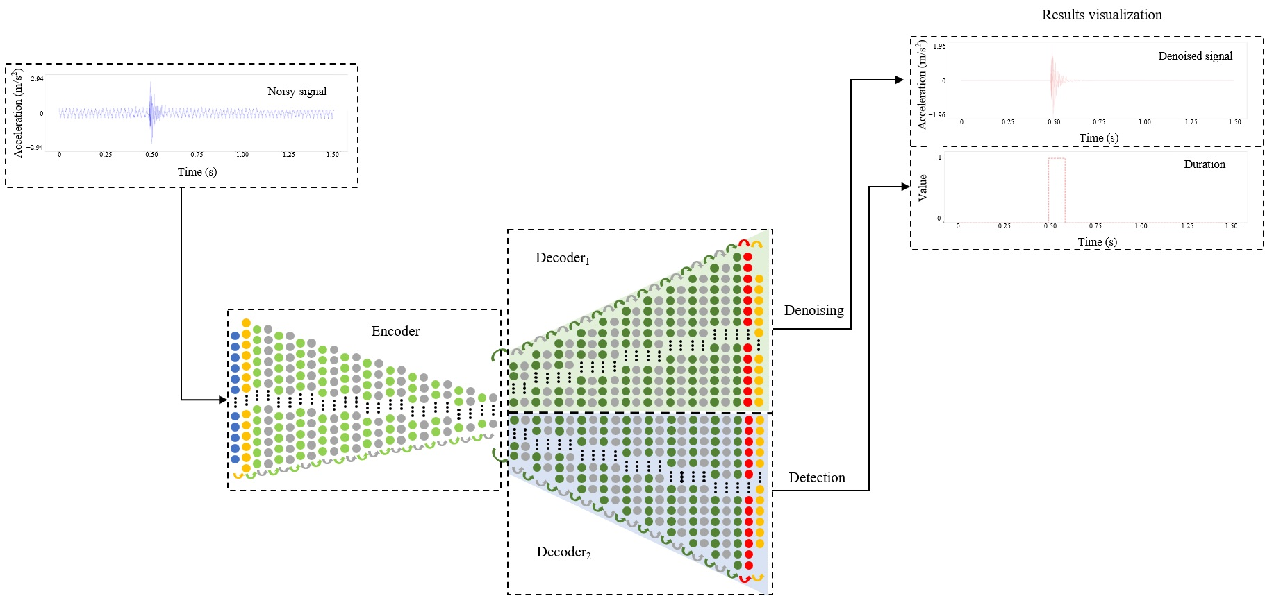
To realize simultaneous microseismic signal denoising and detection, we designed PDTN as a dual-task model. PDTN has three parts, namely an encoder, data with advanced features, and two decoders, as shown in Figure 1a. Encoder E extracted the features of the input data X and generated data H with advanced features. Afterwards, two high-dimensional nonlinear feature maps and were generated by using the parallel decoders D1 and D2 as outputs, respectively, thus allowing PDTN to simultaneously denoise and detect microseismic signals.
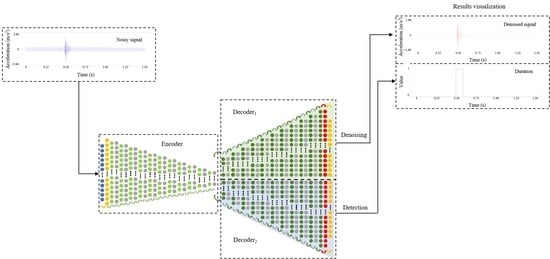
Figure 1b shows the PDTN structure. When using the microseismic signal with noise as input, the size of (30,000, 1) should be reconstructed into (32,768, 1) by filling 0 to prevent dimension mismatch between upsampling and downsampling. A series of coding operations were then performed, and the data were downsampled via a stride 2 convolution. Moreover, one convolution, one batch normalization, and one rectified linear unit (ReLU) were used to increase model nonlinearity, realize information integration, and improve the expression ability of the network. The features of the input data were then extracted. Given the computing time of the convolution layer and ability of the signal to accept nonlocal features, the kernel size of the convolution layer was set to 3. Data with advanced features were used to generate two high-dimensional nonlinear feature maps using two identical decoders. The decoding process involves upsampling, convolution, batch standardization, and using ReLU for mapping information to higher dimensions. To improve the convergence of training and achieve good signal reconstruction, the corresponding feature maps should be concatenated in the encoding and decoding processes [31]. The sigmoid activation function was set in the penultimate layer of the two decoders to generate the mask and label, and the predicted mask and predicted label were then obtained by reconstructing (32,768, 1) into (30,000, 1). Table 1 presents some network structures and parameters in the encoder. With the number of convolutions increasing with stride 2, the output features were gradually compressed, and the network depth gradually increased. To achieve optimal denoising and detection performance, the Bayesian optimization method was applied to optimize the network depth hyperparameter in the convolutional neural network. The Gaussian process regression for modelling the objective function is called a proxy function, and EI is selected as a collection function for selecting the next observation point. When the requirement of minimizing val_loss is met, the regression parameter is output. The network val_loss is small for current sampling times of 9–13. Downsampling times of 9, 10, 11, 12, and 13 were tested (Table 2) to verify their influence on the model. The results demonstrate that PDTN yields the best detection performance in the verification set when the downsampling number is 9. Meanwhile, when the downsampling number is 13, PDTN yields the best denoising performance in the verification set. To consider both the PDTN denoising and detection performance, the network corresponding to a downsampling number of 11, which had the smallest total loss in the verification set, was considered as the research object.
Figure 1c presents the flow chart of denoising and detection via PDTN. First, samples of noisy signals in the time domain were taken as input, and PDTN then simultaneously generated the predicted mask and predicted label . The predicted microseismic signal was obtained by multiplying the predicted mask by noisy signal , and the predicted label denotes the predicted duration of the microseismic signal.
PDTN can automatically learn features from semi-synthetic noisy signals by using one encoder and two identical decoders. Unlike traditional methods, this model does not need to set thresholds to improve its denoising and detection accuracy. A noisy signal input can simultaneously generate two outputs, namely the mask and label, and realize the denoising and detection of microseismic signals, thus improving the efficiency of microseismic signal processing. PDTN can also denoise and detect noisy signals directly in the time domain without signal conversion.
In this paper, the amplitude of all microseismic signals was expressed in terms of acceleration with a response frequency ranging from 50 Hz to 5 kHz. The data acquisition station had a sampling frequency of 20 kHz and a sampling window of 1.5 s for all signals. The data acquisition station had a sampling frequency of 20 kHz and a sampling window of 1.5 s for all signals. Clean microseismic signals are necessary for neural network training, but the field data all contain some noise. We obtain clean microseismic signals in the following way. First, we manually detect the microseismic signal to determine the effective microseismic signal range. The peak amplitude within the effective microseismic signal range is taken as the peak amplitude of the microseismic signal, and the peak amplitude outside the effective microseismic signal range is taken as the peak amplitude of the noise. Then, the approximate SNR can be calculated. The SNR was calculated as follows [32]:
where and denote the peak amplitudes of the microseismic signal and noise. The SNR can reflect the quality of the signal. We select microseismic signals with SNR greater than 30 dB, which are rarely disturbed by noise. We set all the values outside the effective microseismic signal range of these signals to 0 and retain the values within the effective microseismic signal range so that approximate clean microseismic signals can be obtained. The collected dataset contained 9507 microseismic signals and 16,861 noises, randomly divided into training (80%), verification (10%), and test sets (10%). The noise samples were randomly selected and superimposed with the selected microseismic signals to obtain noisy signals with different SNRs as inputs. During training, the Adam optimiser was used to minimise the loss function and update the weight parameters. The learning rate was initially set to 0.0001. After 10 epochs, if the model no longer exhibits improvements, the model should be retrained by multiplying the original learning rate by 0.9. If the loss does not drop after 300 epochs, then training should be stopped.
3. Results
3.1. Test Results
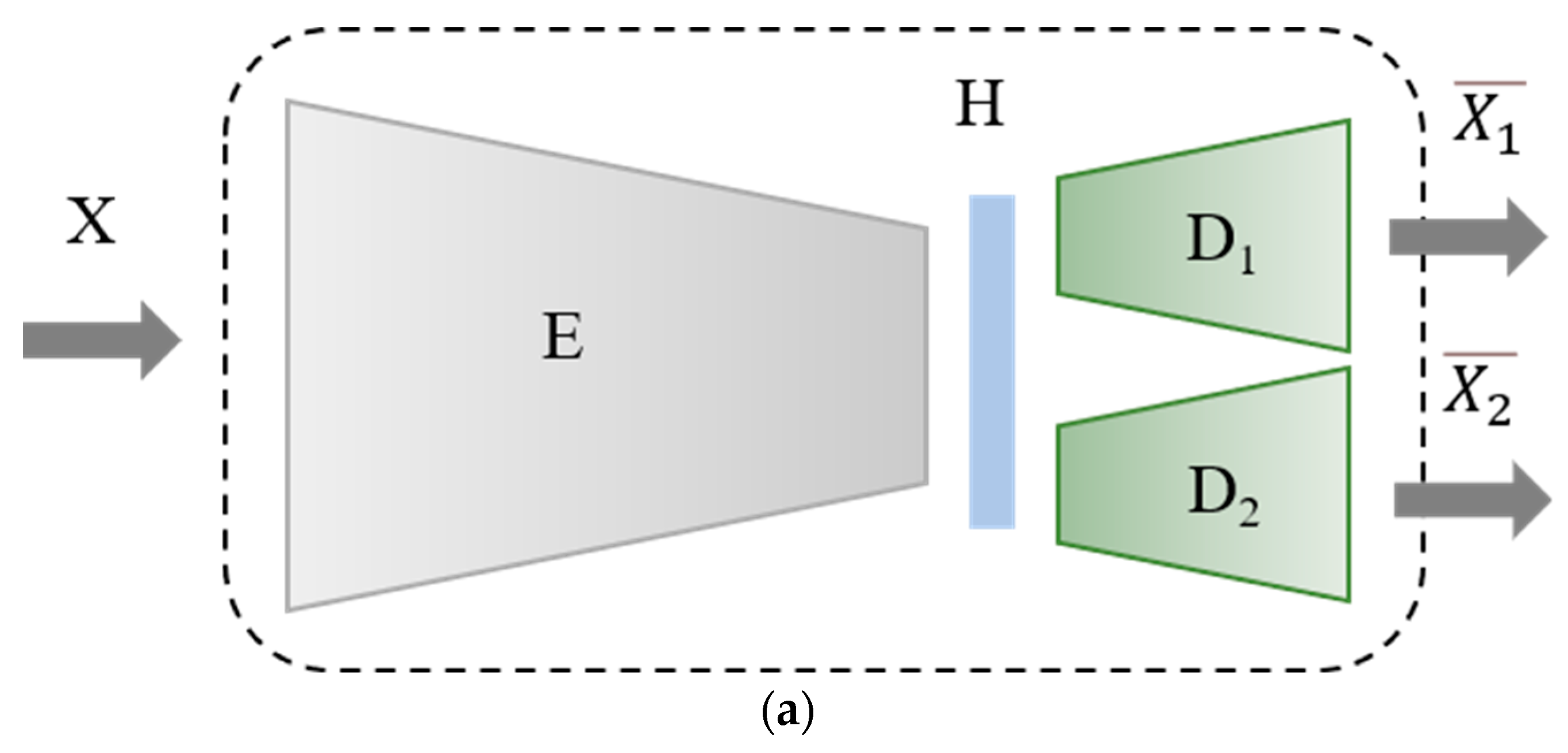
The performance of the PDTN model in the test set is visualised in Figure 2a–g to intuitively convey the denoising and detection performance.
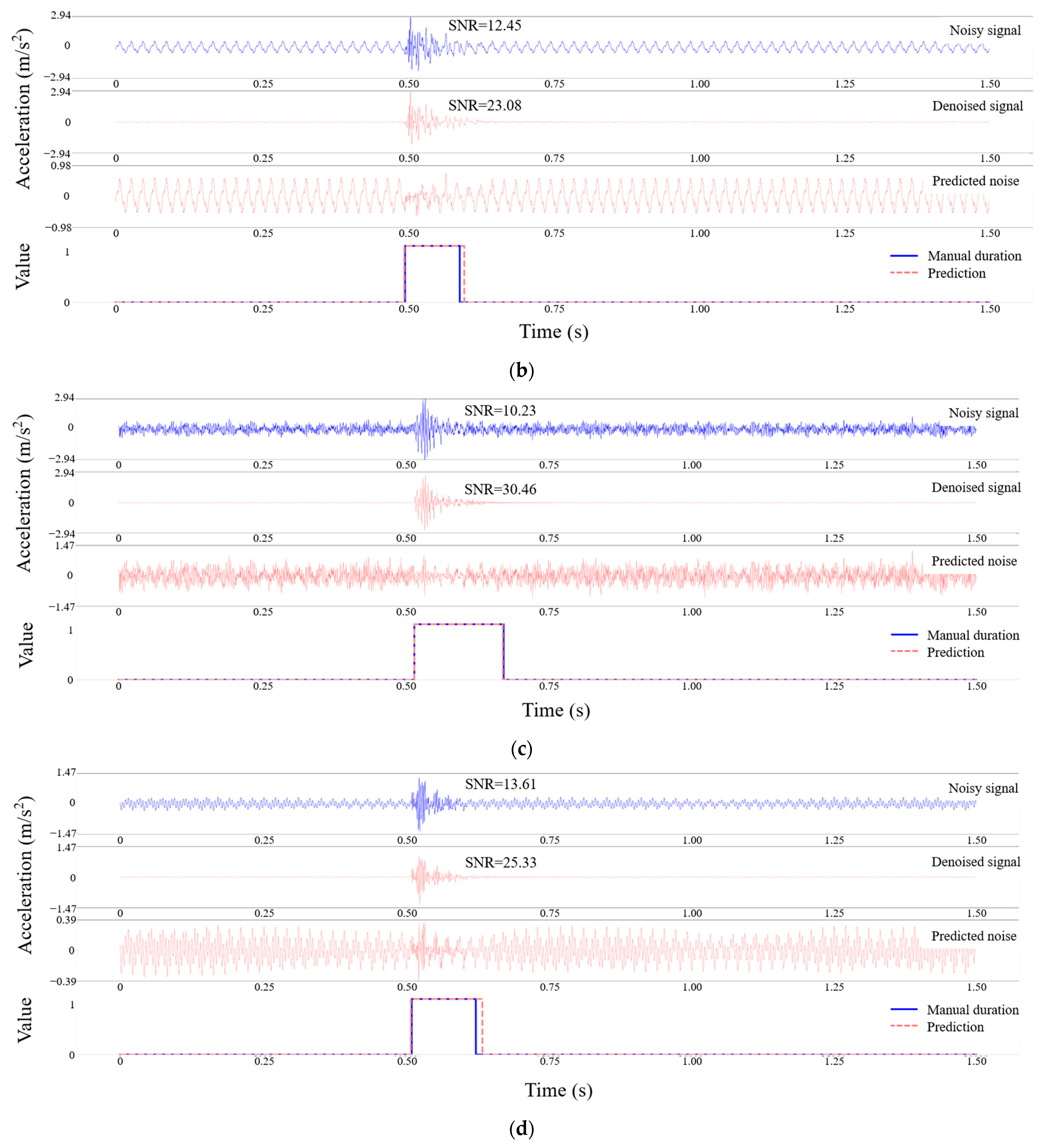
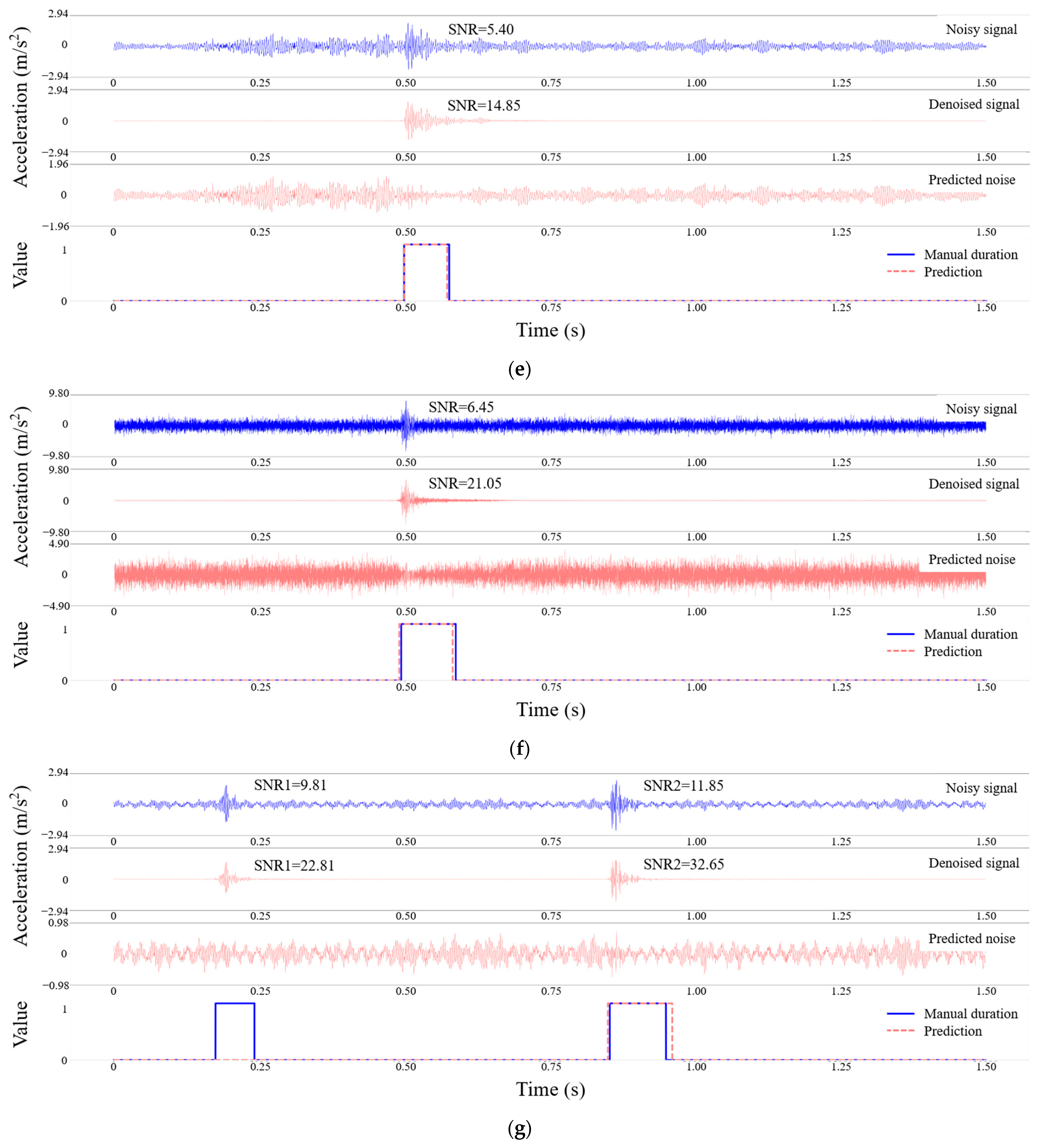
The noise carried by the noisy signals in Figure 2a,c was a mix of cyclic and other noises, whereas it comprised cyclic noises of different frequencies in Figure 2b,d. Figure 2a–d show the actual effects of different noises on the PDTN model and validate its effectiveness in denoising different noisy signals. Noticeably, considerable improvements in SNR were achieved. The noise of the noisy signal in Figure 2e was composed of different kinds of noise whose amplitudes vary greatly. The maximum amplitude of the noise was close to that of the microseismic signal, which results in a low SNR of the microseismic signal. This kind of noise is difficult to be separated, but the PDTN model can still effectively denoise this complex mixed noise and improve the SNR. The noises in Figure 2a–e were all non-Gaussian noises. We further tested the processing effect of PDTN on microseismic signals with Gaussian noise. The noise carried by the noisy signals in Figure 2f was Gaussian noise. PDTN accurately detected the microseismic signal with Gaussian noise, and the SNR of the signal was significantly improved after denoising. The proposed model not only successfully separated the noisy signals from the denoised signals and prediction noises, but also reduced the leakage of microseismic signals after denoising. The predicted noise had a slight waveform distortion in the microseismic signal range. We have avoided intercepting two or more microseismic events into the same sampling window when intercepting the sampling window. Nevertheless, we show the situation in Figure 2g. The noisy signal in Figure 2g contained two microseismic waveforms, making denoising and detection more difficult. As shown in Figure 2g, the PDTN model can successfully separate the noisy signal into denoised signal and predicted noise, even though it contains two microseismic waveforms. The SNR of two microseismic signals was greatly improved. However, the PDTN model only accurately detected one waveform with a larger amplitude, ignoring the microseismic signal with a smaller amplitude.
Manually marking the signal duration yields subjective end times due to the presence of noise. To standardize the manual duration and minimize the influence of subjective factors on the model performance evaluation, the distance between the onset time and end time in the manual duration was set to eight times the distance between the onset time and maximum amplitude point [33]. Thus, most of the microseismic signals can be well covered. The results reveal that the noisy signals are precisely detected by the PDTN regardless of their type when there is one microseismic waveform in the sampling window. When there are two or more microseismic waveforms in the sampling window, PDTN can only accurately detect the one with the largest amplitude. This is because when we train the neural network, the noise signals all contain a microseismic waveform.
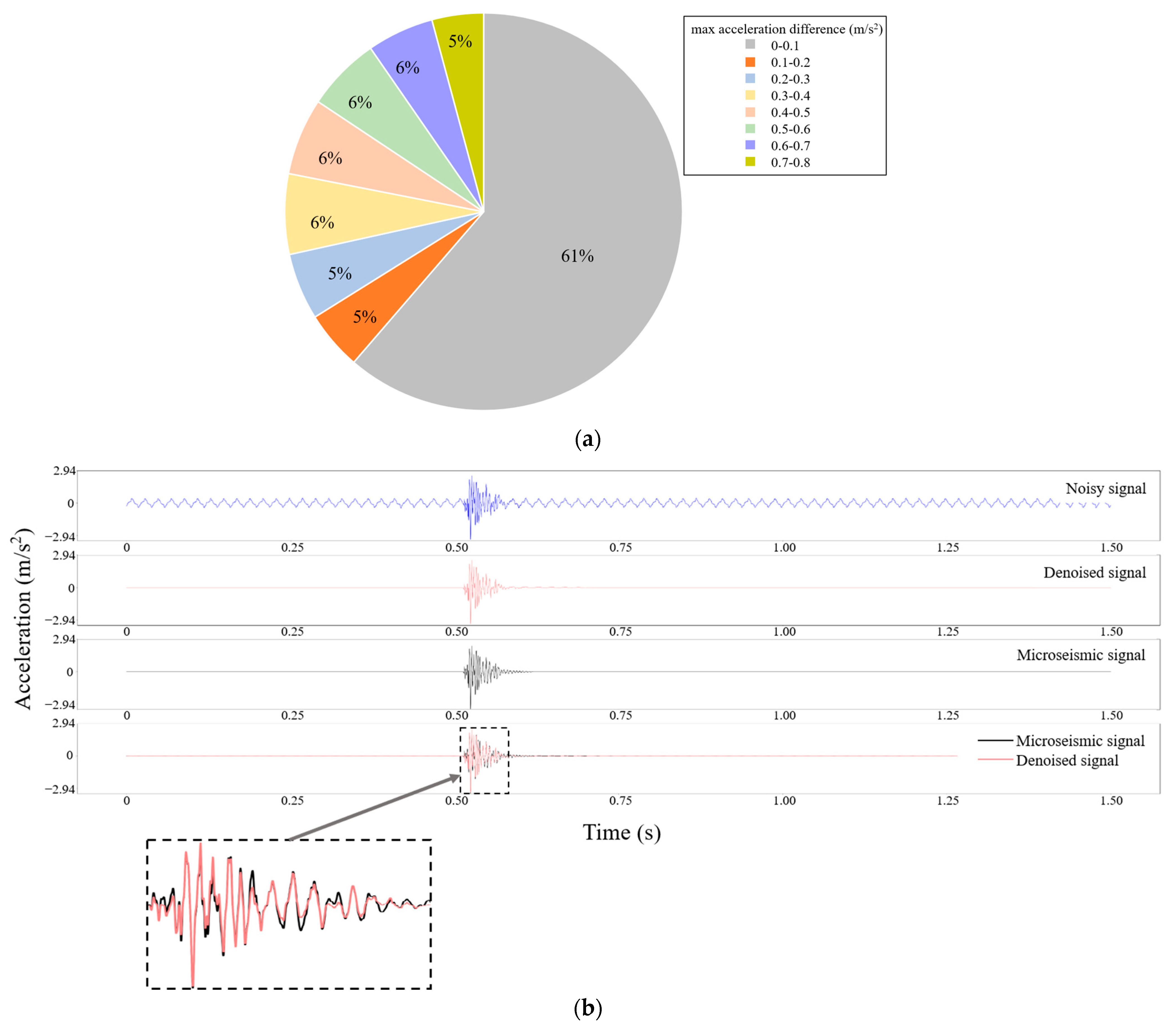
To determine the waveform distortion after PDTN denoising, 2172 noise samples, comprising cyclic and mixed noises from the China Grand Canyon Tunnel, were collected and tested. Figure 3a shows the maximum amplitude difference between the actual and predicted noises. The maximum amplitude difference in more than 61% of the samples was less than 0.1 m/s2, and the average maximum amplitude difference was 0.186 m/s2. Figure 3b compares the waveforms of the denoised and clean microseismic signals. The waveform of the denoised microseismic signal after local amplification was very similar to that of the clean microseismic signal, and the distortion was small. Therefore, using PDTN for denoising produces only slight waveform distortions.
3.2. Application in Real Projects
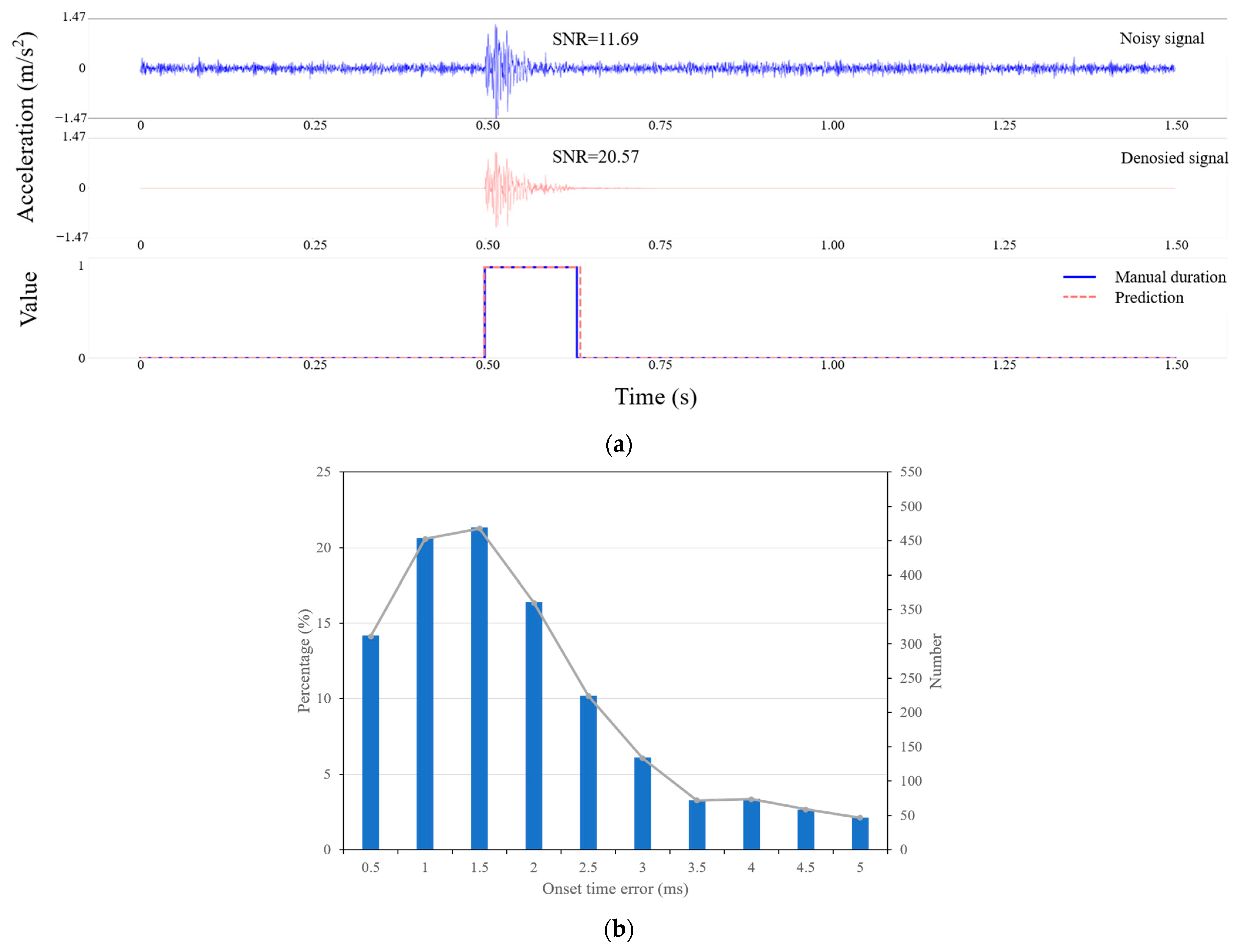
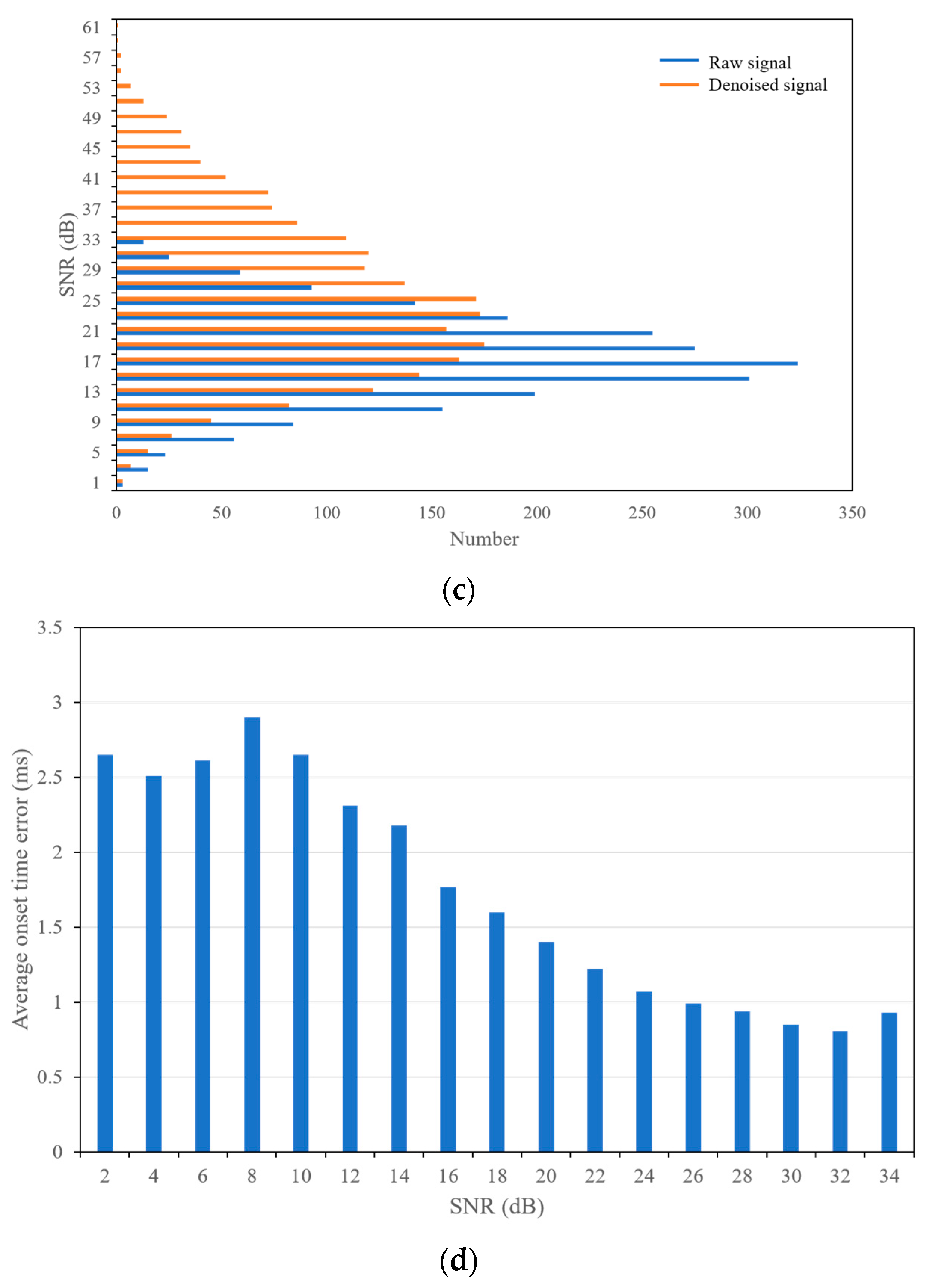
The data used in model training and testing contained noise and clean microseismic signals, and the PDTN model achieved excellent denoising and detection results. To verify the denoising and detection performance of the PDTN model under actual conditions, it was used to detect and denoise 2207 noisy signals collected from the Grand Canyon Tunnel in Sichuan, China. The verification results are shown in Figure 4a. The SNR of the microseismic signals was significantly improved after denoising, whereas the detection accuracy of the microseismic signals was high. Notably, determining the onset time of microseismic signals is critical to locating microseismic events. Figure 4b shows the distribution of the onset time differences of 2207 noisy signals captured manually and using the PDTN model. The PDTN average time pickup error of the microseismic signals was 1.6 ms, and 88.58% of the pickup errors of noisy microseismic signals were less than 1.5 ms. Figure 4c shows the SNR distribution before and after denoising. The average SNR of the microseismic signals increased by 7.28 dB, and the maximum SNR increased by 39.55 dB. The SNR of 2207 microseismic signals with noise was distributed between 0 dB and 34 dB, which were then divided into 17 intervals to study the relationship between SNR and pickup error. Figure 4d shows that a higher SNR corresponds to a smaller pickup error. Specifically, an SNR greater than 20 dB corresponds to a pickup error of less than 1.5 ms. Even at a very low SNR, the maximum pick error was less than 3 ms. Therefore, the PDTN model maintains a good onset time pickup performance even at low SNR. Although the PDTN was trained on semisynthetic microseismic signal sets, it is applicable to real microseismic signals.
4. Discussion
To compare the denoising and detection performance of PDTN with those of traditional methods, a clean microseismic signal was superimposed on a clean noise to generate a noisy signal, and the amplitude of noise was scaled and contracted to generate a noisy signal with different SNRs (Figure 5). The SNR distribution of these noisy signals ranged from 1.61 dB to 31.52 dB. We compared the denoising performance of PDTN, high-pass filter, and feed-forward denoising convolutional neural networks (DnCNN) by taking these noisy signals as input. The onset time picking effects of PDTN and STA/LTA were also compared.
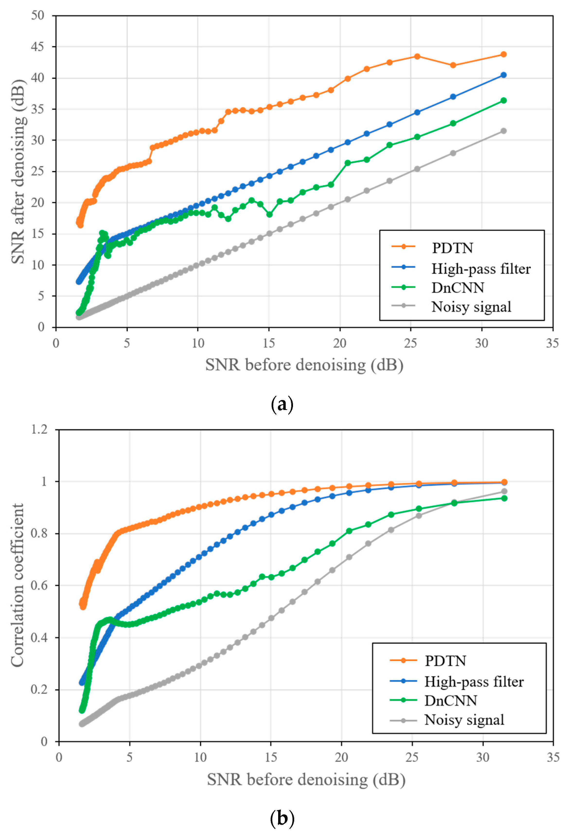
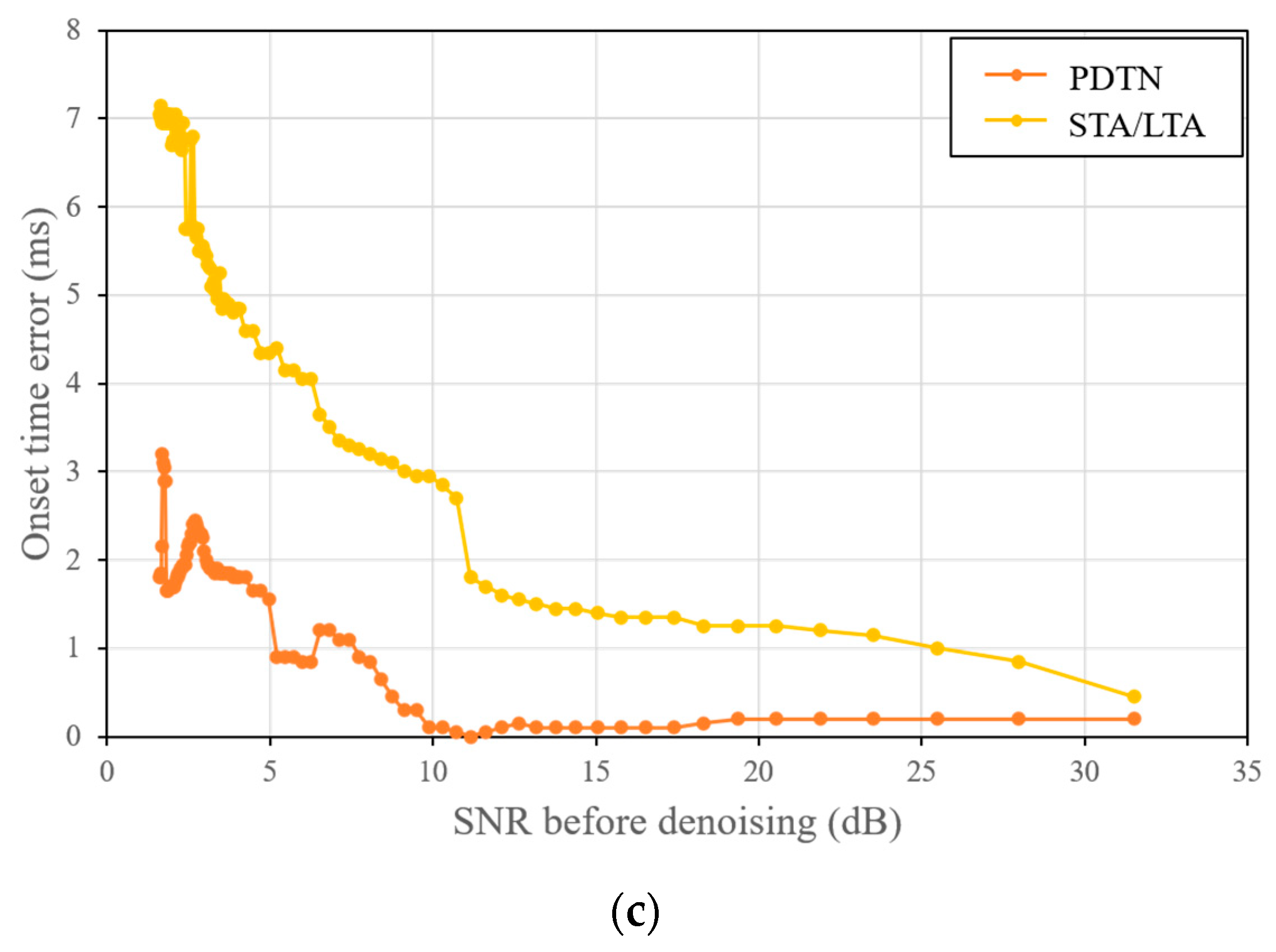
Considering the frequency distribution of the clean microseismic signal and clean noise, the cutoff frequency of the high-pass filter was set to 80 Hz to achieve the best denoising effect. For STA/LTA, the optimal threshold was selected to achieve the most accurate onset time pickup. Figure 6a shows the SNR curve after denoising using PDTN and the high-pass filter. Figure 6a shows the SNR curve after denoising using PDTN, high-pass filter, and DnCNN. The average SNR of the noisy signals was 6.55 dB. The average SNR of the signals denoised using the high-pass filter, DnCNN, and PDTN was 15.02 dB, 12.54 dB, and 25.51 dB, respectively. Compared with the DnCNN, the PDTN improved the SNR by 12.97 dB on average and achieved better denoising effect in the entire SNR range. Compared with the high-pass filter, the PDTN improved the SNR by 10.49 dB on average and achieved better denoising effect in the entire SNR range. The correlation coefficient can indicate the correlation among signals. The closer the correlation coefficient is to 1, the greater the similarity between two signals. The correlation coefficients between the clean microseismic signal and the signal denoised using PDTN, high-pass filter, and DnCNN were calculated to determine the influence of their denoising performance on the waveform. The correlation coefficient was expressed as a Pearson product–moment correlation coefficient [34]. Figure 6b shows the correlation coefficient curve. For the high-SNR case, the correlation coefficients of the microseismic signal after denoising using PDTN and the high-pass filter both approached 1. However, for the low-SNR case, the correlation coefficients of the microseismic signal denoised using PDTN were much higher than those obtained after denoising using the high-pass filter. This suggests that the microseismic signal can maintain high fidelity after PDTN denoising under a low SNR and that the waveform is closer to the clean microseismic signal. The correlation coefficients of the microseismic signal denoised by DnCNN were far worse than those denoised using PDTN under any SNR condition, indicating that DnCNN denoising significantly distorts the waveform. PDTN and STA/LTA were then used to extract the onset time of the noisy signals, and the error curve is shown in Figure 6c. When the SNR was less than 12 dB, the STA/LTA pickup error sharply increased, indicating that this algorithm is not suitable for low-SNR conditions. However, when the SNR was greater than 10 dB, the mean onset time error of PDTN was only 0.13 ms. Although the pickup accuracy decreases with the SNR of noisy signals, the maximum PDTN pickup error remained within 3.2 ms. Therefore, PDTN outperformed STA/LTA under both low- and high-SNR conditions. The average onset time error of PDTN was 1.41 ms, whereas that of STA/LTA was 4.65 ms, suggesting that the pickup accuracy of PDTN was much higher than that of STA/LTA.
We used Precision, Recall, and F1-score parameters to further compare and evaluate model performance.
where TP, FP, and FN represent true positive, false positive, and false negative, respectively. Precision is the ratio of TP and total of predicted positives. Recall is the ratio of TP and total of all actual positives. F1-score is the harmonic mean of Precision and Recall. Since the sampling frequency is 20 kHz, a pick is considered a true positive when the onset time error is less than 2.5 ms. The two confusion matrices obtained according to PDTN and STA/LTA pickup results are shown in Table 3 and Table 4. Precision, Recall, and F1-score of the two methods can be calculated from Table 3 and Table 4, as shown in Table 5. Results in Table 5 show that the Precision and F1-score of PDTN are higher than those of STA/LTA, suggesting that the pickup accuracy of PDTN was much higher than that of STA/LTA.
Under different SNR conditions, PDTN achieved a much better denoising effect and onset time pickup accuracy compared with the high-pass filter, DnCNN, and STA/LTA. It also avoids the complicated step of utilizing different denoising methods for different types of noises and does not require an artificial threshold to improve its denoising effect and detection accuracy.
Denoising and detection networks were constructed to compare the efficiency difference between simultaneous denoising and detection using PDTN and those using separate denoising and detection. The denoising network and the detection network have the same structure, as shown in Figure 7, which comprises an encoder and a decoder. Ninety-nine semi-synthetic noise microseismic signals were used as model inputs. The results revealed that the denoising network required 13.69 s, the detection network required 15.12 s, and the total time was 28.81 s. PDTN required 19.65 s, which means that simultaneous denoising and detection using PDTN saved 9.16 s compared with separate denoising and detection. A dual-tasking network consisting of an encoder and two parallel decoders for denoising and detection has fewer parameters than two single-tasking networks because it shares one encoder. Fewer parameters make the dual-tasking network more efficient in testing than the two single-tasking networks. This advantage is amplified when dealing with large amounts of microseismic data. Therefore, PDTN can efficiently denoise and detect microseismic signals simultaneously.
Accurate mask prediction is required to realize the denoising function of the model. However, the mask cannot reflect the clean microseismic signal and noise superposition cancelling the positive and negative amplitudes. Therefore, prediction noise will inevitably appear as waveform distortion in the microseismic signal range, which is a disadvantage associated with masks. Expanding microseismic datasets in the future, especially clean microseismic signal datasets, will facilitate relevant deep learning methods that directly output predicted denoising waveforms, which would effectively improve the shortcomings of this method. When there are two or more microseismic waveforms in the sampling window, PDTN can only accurately detect the one with the largest amplitude. This is the deficiency of the model and the direction of further improvement of the model.
5. Conclusions
The proposed PDTN model is a deep learning model that can efficiently and automatically detect microseismic data. This model has a dual-task structure comprising an encoder and two parallel decoders. Two outputs are simultaneously generated to facilitate the simultaneous denoising and detection of microseismic signals in the time domain.
- This model exhibits excellent denoising abilities, which can improve the SNR of microseismic signals containing different types of noise. Compared with the high-pass filter, the SNR is improved by 10.49 dB on average after denoising using PDTN. Compared with DnCNN, the SNR is improved by 12.97 dB on average after denoising using PDTN. The correlation coefficient between the signal denoised using PDTN and the original microseismic signal is higher in all SNR conditions, indicating that the denoised waveform distortion by PDTN is smaller.
- The model exhibits good detection ability: it accurately detects noisy microseismic signals with different SNRs. Compared with STA/LTA, the initial time error of this method is reduced by 3.24 ms, and its error remains below 3.2 ms at the low SNR.
- Denoising and detection efficiency using PDTN is higher than that for separate denoising and detection. When using 99 microseismic signals as input, the results reveal that the simultaneous denoising and detection using PDTN save 9.16 s compared with separate denoising and detection.
- PDTN can denoise and detect various noisy microseismic signals without requiring parameter adjustment for different signals. PDTN meets the demand for automatically processing massive microseismic data, and this method has great potential in data processing for exploration seismology, and earthquake and disaster assessment.
Author Contributions
Conceptualization, C.M.; Data curation, W.Y. and X.R.; Formal analysis, W.Y. and X.R.; Funding acquisition, C.M.; Investigation, W.Y. and C.M.; Methodology, C.M. and W.Y.; Project administration, T.L.; Resources, C.M. and T.L.; Software, W.Y. and W.X.; Supervision, T.L.; Validation, J.W. and K.T.; Visualization, W.Y. and Y.L.; Writing—original draft, W.Y. and C.M.; Writing—review and editing, W.X. and J.W. All authors have read and agreed to the published version of the manuscript.
Funding
This work was financially supported by the National Natural Science Foundation of China (grant number 42177173), State Key Laboratory of Geohazard Prevention and Geoenvironment Protection Independent Research Project (grant number SKLGP2020Z010).
Data Availability Statement
The data presented in this study are available on request from the corresponding author.
Acknowledgments
We appreciate the microseismic monitoring staff at Micangshan Tunnel and Grand Canyon Tunnel. We also appreciate the support of Sichuan Road and Bridge Group Co., Ltd. and Sichuan Bashan Expressway Co. LTD.
Conflicts of Interest
The authors declare no conflict of interest.
References
- Feng, G.L.; Feng, X.T.; Chen, B.R.; Xiao, Y.X.; Zhao, Z.N. Effects of structural planes on the microseismicity associated with rockburst development processes in deep tunnels of the Jinping-II Hydropower Station, China. Tunn. Undergr. Space Technol. 2019, 84, 273–280. [Google Scholar] [CrossRef]
- Feng, G.L.; Feng, X.T.; Chen, B.R.; Xiao, Y.X.; Liu, G.F.; Zhang, W.; Hu, L. Characteristics of Microseismicity during Breakthrough in Deep Tunnels: Case Study of Jinping-II Hydropower Station in China. Int. J. Geomech. 2020, 20, 04019163. [Google Scholar] [CrossRef]
- Ma, K.; Liu, G.Y. Three-Dimensional Discontinuous Deformation Analysis of Failure Mechanisms and Movement Characteristics of Slope Rockfalls. Rock Mech. Rock Eng. 2022, 55, 275–296. [Google Scholar] [CrossRef]
- Zhang, H.; Zeng, J.; Ma, J.J.; Fang, Y.; Ma, C.C.; Yao, Z.G.; Chen, Z.Q. Time Series Prediction of Microseismic Multi-parameter Related to Rockburst Based on Deep Learning. Rock Mech. Rock Eng. 2021, 54, 6299–6321. [Google Scholar] [CrossRef]
- Ma, C.C.; Li, T.B.; Zhang, H. Microseismic and precursor analysis of high-stress hazards in tunnels: A case comparison of rockburst and fall of ground. Eng. Geol. 2020, 265, 105435. [Google Scholar] [CrossRef]
- Wamriew, D.; Dorhjie, D.B.; Bogoedov, D.; Pevzner, R.; Maltsev, E.; Charara, M.; Pissarenko, D.; Koroteev, D. Microseismic Monitoring and Analysis Using Cutting-Edge Technology: A Key Enabler for Reservoir Characterization. Remote Sens. 2022, 14, 3417. [Google Scholar] [CrossRef]
- Hu, R.; Wang, Y. A first arrival detection method for low SNR microseismic signal. Acta Geophys. 2018, 66, 945–957. [Google Scholar] [CrossRef]
- Li, J.; Li, Y.; Li, Y.; Qian, Z.H. Downhole Microseismic Signal Denoising via Empirical Wavelet Transform and Adaptive Thresholding. J. Geophys. Eng. 2018, 15, 2469–2480. [Google Scholar] [CrossRef] [Green Version]
- Mallat, S.; Hwang, W.L. Singularity detection and processing with wavelets. IEEE Trans. Inf. Theory 1992, 38, 617–643. [Google Scholar] [CrossRef]
- Tang, S.; Tong, M.; He, X. The Optimum Wavelet Base of Wavelet Analysis in Coal Rock Microseismic Signals. Adv. Mech. Eng. 2014, 6, 967952. [Google Scholar] [CrossRef]
- Han, J.; Mirko, V.D.B. Microseismic and seismic denoising via ensemble empirical mode decomposition and adaptive thresholding. Geophysics 2015, 80, KS69–KS80. [Google Scholar] [CrossRef] [Green Version]
- Li, X.B.; Zhang, Y.P.; Zuo, Y.J.; Wang, W.H. Filtering and denoising of rock blasting vibration signal with EMD. J. Cent. South Univ. Sci. Technol. 2006, 37, 150–154. (In Chinese) [Google Scholar] [CrossRef]
- Li, X.; Dong, L.L.; Li, B.; Lei, Y.F.; Xu, N.W. Microseismic Signal Denoising via Empirical Mode Decomposition, Compressed Sensing, and Soft-thresholding. Appl. Sci. 2020, 10, 2191. [Google Scholar] [CrossRef] [Green Version]
- Daubechies, I.; Lu, J.; Wu, H.T. Synchrosqueezed wavelet transforms: An empirical mode decomposition-like tool. Appl. Comput. Harmon. Anal. 2011, 30, 243–261. [Google Scholar] [CrossRef] [Green Version]
- Ruan, W.Y.; Ma, Z.Q.; Chen, M.Y.; Zhang, A. A Method to Improve Noise Robustness of Synchrosqueezing Transform. J. Univ. Jinan Sci. Technol. 2019, 33, 42–49. (In Chinese) [Google Scholar] [CrossRef]
- Wang, C.; Wang, W.H. Optimal method of SVD for microseismic data based on background noise and eigenvalue ratio of reduction. J. Northeast Pet. Univ. 2020, 44, 13. (In Chinese) [Google Scholar] [CrossRef]
- Li, X.B.; Shang, X.Y.; Wang, Z.W.; Dong, L.J.; Weng, L. Identifying P-phase arrivals with noise: An improved Kurtosis method based on DWT and STA/LTA. J. Appl. Geophys. 2016, 133, 50–61. [Google Scholar] [CrossRef]
- Li, S.C.; Cheng, S.; Li, L.P.; Shi, S.S.; Zhang, M.G. Identification and Location Method of Microseismic Event Based on Improved STA/LTA Algorithm and Four-Cell-Square-Array in Plane Algorithm. Int. J. Geomech. 2019, 19, 04019067.1–04019067.8. [Google Scholar] [CrossRef]
- Stevenson, R. Microearthquakes at Flathead Lake, Montana: A study using automatic earthquake processing. Bull. Seismol. Soc. Am. 1976, 66, 61–79. [Google Scholar] [CrossRef]
- Li, X.L.; Liu, X.Q.; Dong, X.N.; Xu, D. Application and Expectation of Higher-order Statistics in Geophysics. Northwest. Seismol. J. 2010, 32, 201–205. (In Chinese) [Google Scholar] [CrossRef]
- Liu, J.S.; Wang, Y.; Yao, Z.X. On micro-seismic first arrival identification A case study. Chin. J. Geophys. 2013, 56, 1660–1666. (In Chinese) [Google Scholar] [CrossRef]
- Saragiotis, C.D.; Hadjileontiadis, L.J.; Panas, S.M. PAI-S/K: A Robust Automatic Seismic P Phase Arrival Identification Scheme. IEEE Trans. Geosci. Remote Sens. 2002, 40, 1395–1404. [Google Scholar] [CrossRef]
- Chen, H.; Yang, Z. Arrival Picking of Acoustic Emission Signals Using a Hybrid Algorithm Based on AIC and Histogram Distance. IEEE Trans. Instrum. Meas. 2021, 70, 3505808. [Google Scholar] [CrossRef]
- Long, Y.; Lin, J.; Li, B.; Wang, H.C.; Chen, Z.B. Fast-AIC Method for Automatic First Arrivals Picking of Microseismic Event with Multitrace Energy Stacking Envelope Summation. IEEE Geosci. Remote Sens. Lett. 2019, 17, 1832–1836. [Google Scholar] [CrossRef]
- Maeda, N. A method for reading and checking phase times in autoprocessing system of seismic data. Zisin 1985, 38, 365–380. [Google Scholar] [CrossRef] [PubMed] [Green Version]
- Pu, Y.Y.; Apel, D.B.; Liu, V.; Mitri, H. Machine learning methods for rockburst prediction-state-of-the-art review. Int. J. Min. Sci. Technol. 2022, 29, 565–570. [Google Scholar] [CrossRef]
- Zhong, T.; Cheng, M.; Dong, X.T.; Li, Y.; Wu, N. Seismic random noise suppression by using deep residual U-Net. J. Pet. Sci. Eng. 2021, 209, 109901. [Google Scholar] [CrossRef]
- Zhu, W.; Mousavi, S.M.; Beroza, G.C. Seismic Signal Denoising and Decomposition Using Deep Neural Networks. IEEE Trans. Geosci. Remote Sens. 2018, 57, 9476–9488. [Google Scholar] [CrossRef] [Green Version]
- Mousavi, S.M.; Ellsworth, W.L.; Zhu, W.; Chuang, L.Y.; Beroza, G.C. Earthquake transformer—An attentive deep-learning model for simultaneous earthquake detection and phase picking. Nat. Commun. 2020, 11, 3952. [Google Scholar] [CrossRef]
- Zhang, J.L.; Sheng, G.Q. First arrival picking of microseismic signals based on nested U-Net and Wasserstein Generative Adversarial Network. J. Pet. Sci. Eng. 2020, 195, 107527. [Google Scholar] [CrossRef]
- Ronneberger, O.; Fischer, P.; Brox, T. U-Net: Convolutional Networks for Biomedical Image Segmentation. In Proceedings of the Medical Image Computing and Computer-Assisted Intervention–MICCAI 2015: 18th International Conference, Munich, Germany, 5–9 October 2015; Springer: Berlin/Heidelberg, Germany, 2015. [Google Scholar] [CrossRef] [Green Version]
- Mousavi, S.M.; Zhu, W.Q.; Sheng, Y.X.; Beroza, G.C. Cred: A deep residual network of convolutional and recurrent units for earthquake signal detection. Sci. Rep. 2019, 9, 10267. [Google Scholar] [CrossRef] [PubMed] [Green Version]
- Zhang, H.; Ma, C.; Jiang, Y.; Casagli, N. Integrated Processing Method for Microseismic Signal Based on Deep Neural Network. Geophys. J. Int. 2021, 226, 2145–2157. [Google Scholar] [CrossRef]
- Mantovani, E.; Albarello, D.; Mucciarelli, M. Seismic activity in North Aegean region as middle-term precursor of Calabrian earthquakes. Phys. Earth Planet. Inter. 1986, 44, 264–273. [Google Scholar] [CrossRef]
Figure 1.
(a) Schematic of PDTN. (b) Structure diagram of PDTN. Encoder on the left; two decoders on the right; and denoising and detection networks on the top and bottom, respectively. The circles of different colors represent the neural network layer. The arrows represent operations performed between two adjacent layers. The dimensions of each layer are marked as ‘feature × filters’. The encoder performs 11 downsamplings and the two decoders perform 11 upsamplings. The total number of trainable parameters is 47,791,298. (c) Flow chart of PDTN for denoising and detection.


Figure 2.
Visualization of denoising and detection performance of PDTN in the test set. (a–g) Each figure consists of four figures: from top to bottom, respectively, noisy signal, denoised signal, predicted noise, and manual and predicted durations.
Figure 2.
Visualization of denoising and detection performance of PDTN in the test set. (a–g) Each figure consists of four figures: from top to bottom, respectively, noisy signal, denoised signal, predicted noise, and manual and predicted durations.


Figure 3.
(a) Maximum amplitude difference distribution between noise and predicted noise. (b) The contrast diagram of the waveform of the PDTN denoised microseismic signal and the waveform of the clean microseismic signal. From top to bottom, the noisy signal (composed of the original clean microseismic signal and noise), PDTN denoised microseismic signal, clean microseismic signal, comparison between the PDTN denoised microseismic signal and the clean microseismic signal, and the local magnification.

Figure 4.
(a) Visualization of denoising and detection performance of PDTN in the Grand Canyon tunnel data set. It consists of three graphs: from top to bottom, noisy signal, denoised signal, and manual and predicted durations, respectively. (b) Error distribution diagram of manual and PDTN onset time picking of noisy signals. (c) SNR layout before and after PDTN denoising. (d) The relation between SNR of noise signal and onset time error.


Figure 5.
Composite diagram of noisy signals with different SNRs. (a) Noisy signal SNR of 17.38 dB. (b) Noisy signal SNR of 11.16 dB. (c) Noisy signal SNR of 7.43 dB.
Figure 5.
Composite diagram of noisy signals with different SNRs. (a) Noisy signal SNR of 17.38 dB. (b) Noisy signal SNR of 11.16 dB. (c) Noisy signal SNR of 7.43 dB.

Figure 6.
Contrast diagram of PDTN, DnCNN, high-pass filter, and STA/LTA denoising and onset time picking effect. (a) SNR curves of noisy signals and signals denoised using PDTN, DnCNN, and high-pass filtering. (b) The correlation coefficients between the clean microseismic signal and the signal denoised using the high-pass filter, DnCNN, and PDTN. (c) The onset time error of noisy signals detected using PDTN and STA/LTA.


Figure 7.
Structure diagram of denoising and detection models for model efficiency comparison. The circles of different colors represent the neural network layer. The arrows represent operations performed between two adjacent layers. The dimensions of each layer are marked as ‘feature × filters’.
Figure 7.
Structure diagram of denoising and detection models for model efficiency comparison. The circles of different colors represent the neural network layer. The arrows represent operations performed between two adjacent layers. The dimensions of each layer are marked as ‘feature × filters’.


Table 1.
Partial network structure and parameters in encoder.
| Type | Kernel Size/Stride | Output Shape |
|---|---|---|
| Lambda | 32,768 × 1 | |
| Convolution | 1 × 3/2 | 16,384 × 64 |
| Batch Normalization | 16,384 × 64 | |
| ReLU | 16,384 × 64 | |
| Convolution | 1 × 3/1 | 16,384 × 64 |
| Batch Normalization | 16,384 × 64 | |
| ReLU | 16,384 × 64 | |
| Convolution | 1 × 3/2 | 8192 × 128 |
| Batch Normalization | 8192 × 128 | |
| ReLU | 8192 × 128 | |
| Convolution | 1 × 3/1 | 8192 × 128 |
| Batch Normalization | 8192 × 128 | |
| ReLU | 8192 × 128 |
Note. Output Shape is ‘feature × filters’.
Table 2.
Performance of PDTN with different downsampling times for the verification set.
| Number | Val_Loss | Val_Accuracy | |||
|---|---|---|---|---|---|
| Denoising | Detection | Total | Denoising | Detection | |
| 9 | 0.0547 | 0.0338 | 0.0885 | 0.9606 | 0.9576 |
| 10 | 0.0540 | 0.0466 | 0.1006 | 0.9639 | 0.9319 |
| 11 | 0.0484 | 0.0397 | 0.0881 | 0.9626 | 0.9448 |
| 12 | 0.0504 | 0.0387 | 0.0892 | 0.9619 | 0.9467 |
| 13 | 0.0469 | 0.0419 | 0.0887 | 0.9667 | 0.9429 |
Note. Number represents the number of convolutions with stride 2 in the encoder. Val_loss and val_accuracy are the loss and accuracy of the verification set, respectively. Total val_loss is equal to denoising val_loss plus detection val_loss.
Table 3.
The confusion matrix obtained according to PDTN pickup results.
| Actual | Positive | Negative | |
|---|---|---|---|
| Predict | |||
| Positive | 94 | 5 | |
| Negative | 0 | 0 | |
Table 4.
The confusion matrix obtained according to STA/LTA pickup results.
| Actual | Positive | Negative | |
|---|---|---|---|
| Predict | |||
| Positive | 19 | 80 | |
| Negative | 0 | 0 | |
Table 5.
The comparison of onset time picking between PDTN and STA/LTA.
| Methods | Precision | Recall | F1-Score |
|---|---|---|---|
| PDTN | 0.949 | 1 | 0.974 |
| STA/LTA | 0.192 | 1 | 0.322 |
Disclaimer/Publisher’s Note: The statements, opinions and data contained in all publications are solely those of the individual author(s) and contributor(s) and not of MDPI and/or the editor(s). MDPI and/or the editor(s) disclaim responsibility for any injury to people or property resulting from any ideas, methods, instructions or products referred to in the content. |
© 2023 by the authors. Licensee MDPI, Basel, Switzerland. This article is an open access article distributed under the terms and conditions of the Creative Commons Attribution (CC BY) license (https://creativecommons.org/licenses/by/4.0/).
Share and Cite
MDPI and ACS Style
Ma, C.; Yan, W.; Xu, W.; Li, T.; Ran, X.; Wan, J.; Tong, K.; Lin, Y. Parallel Processing Method for Microseismic Signal Based on Deep Neural Network. Remote Sens. 2023, 15, 1215. https://doi.org/10.3390/rs15051215
AMA Style
Ma C, Yan W, Xu W, Li T, Ran X, Wan J, Tong K, Lin Y. Parallel Processing Method for Microseismic Signal Based on Deep Neural Network. Remote Sensing. 2023; 15(5):1215. https://doi.org/10.3390/rs15051215
Chicago/Turabian StyleMa, Chunchi, Wenjin Yan, Weihao Xu, Tianbin Li, Xuefeng Ran, Jiangjun Wan, Ke Tong, and Yu Lin. 2023. "Parallel Processing Method for Microseismic Signal Based on Deep Neural Network" Remote Sensing 15, no. 5: 1215. https://doi.org/10.3390/rs15051215
Note that from the first issue of 2016, this journal uses article numbers instead of page numbers. See further details here.