

Ecosystem Service Function Supply–Demand Evaluation of Urban Functional Green Space Based on Multi-Source Data Fusion
1
Aerospace Information Research Institute, Chinese Academy of Sciences, No.9 Dengzhuang South Road, Haidian District, Beijing 100094, China
2
University of Chinese Academy of Sciences, No.19(A) Yuquan Road, Shijingshan District, Beijing 100049, China
3
Department of Geological and Atmospheric Sciences, Iowa State University, Ames, IA 50011, USA
*
Author to whom correspondence should be addressed.
Remote Sens. 2023, 15(1), 118; https://doi.org/10.3390/rs15010118
Submission received: 21 November 2022
/
Revised: 21 December 2022
/
Accepted: 22 December 2022
/
Published: 26 December 2022
(This article belongs to the Special Issue Urban Ecophysiology: A Remote Sensing Perspective)
Abstract
:With the rapid development of urbanization, it is an important goal for urban green space (UGS) to meet the needs of residents’ production and life using a supply–demand evaluation method of ecosystem service (ES). However, most studies have considered all functional types of UGS as the supply side, or rely solely on a single supply or demand side to conduct ecosystem service function (ESF) evaluation, resulting in less accurate and targeted research findings. As a result, a novel methodological framework for matching each ESF with corresponding functional types of UGS, and considering both supply and demand sides have been required. Firstly, the object-oriented approach combining support vector machine (SVM) and normalized difference vegetation index (NDVI) was used to automatically identify UGS, and integrated Point of Interest (POI), urban built-up area, road land, parcel, and socio-economic data to classify six functional types of UGS using the near-convex-hull. Next, matching the functional types of UGS with five ESFs, both supply and demand status were evaluated using the carbon sequestration and release analysis, Gaussian two-step floating catchment area, and spatial equilibrium degree methods. This method was demonstrated in Beijing, China. The results show: (1) the ES supply–demand situation provided by each functional type of UGS is different in five ESFs; (2) considering both supply and demand is more intuitive to see whether the city’s demand for UGS has been met. Our results provide a new perspective for evaluating the contribution of UGS and have practical implications for UGS planning.
1. Introduction
Urban green space (UGS) refers to land with natural vegetation and artificial vegetation as the main form of existence within the administrative area of a city, including land used for greening within the scope of urban construction land and land in areas outside urban construction land with a high degree of greening [1]. According to the type of vegetation, UGS can be classified as trees, shrubs, grasses, etc. [2]. In terms of natural functions, UGS has a vital role in promoting the conservation of biodiversity [3], reducing the urban heat island effect [4], and improving air pollution [5]. In terms of social functions, UGS not only impacts the physiological health of residents [6] but also helps to promote their mental health [7]. Ecosystem service (ES) was named in 1997 [8], and represents the benefits human populations derive, directly or indirectly, from ecosystem functions, and is divided into four main types including supporting, provisioning, regulating and cultural services [9]. A good structure and spatial layout of UGS have a catalytic effect on the synergy of various ESs [10]. However, rapid urbanization has led to a continuous reduction in the amount of land available for UGS, bringing about a rapid increase in carbon emissions and associated climate change risks [11], which has led to a series of problems of supply–demand imbalance and development mismatch for ES [12]. Therefore, in order to plan the pattern and improve the service capacity of UGS, it is a prerequisite to grasp the specific distribution of UGS and to have a clear evaluation of the supply–demand situation of ES in UGS, which is of great significance for sustainable urban development.
Research on UGS in the field of ES has undergone a continuous development process of integrating data from multiple sources. At its simplest, field research has been conducted on a small scale. Feyisa et al. (2014) [13] found that an appropriate choice of species, geometry, and size of parks may improve the cooling effect of UGS through the actual measurement of 21 parks in Addis Ababa, Ethiopia. Ayala-Azcárraga et al. (2019) [14] surveyed users of nine parks in México City, and found that the components of urban parks such as tree abundance, safeness, playground qualities had a close relationship with citizen well-being. With the development of remote sensing technology, remote sensing images were gradually applied to the identification of UGS and the evaluation of related ES on a large scale, which effectively improved the drawbacks of research with subjective errors and heavy workloads. Using the spectral mixture analysis (SMA) model on the large scale of Singapore, Masoudi et al. (2019) [15] found patches of UGS that were simpler in shape, more connected, and less fragmented had better cooling effect. Nesbitt et al. (2019) [16] used aerial imagery and census data to examine the distributional equity of UGS by using Spearman’s correlations and spatial autoregressive models, and found that education and income were most strongly associated with the distribution of UGS. Barbierato et al. (2020) [17] combined remote sensing and proximate sensing (Street View) approaches with data retrieved from Google Street View, and divided urban forest into two categories including green cover on facades and green cover on sky view to quantify urban forest ecosystem services score. Dang et al. (2021) [18] evaluated the value of urban green ecological landscape aesthetics on the basis of combining the normalized vegetation index (NDVI) calculated by the satellite remote sensing image with the Tencent panoramic green view index (TP_GVI) calculated by the urban streetscape images. Later, social perception data such as Point of Interest (POI) were applied to the study of UGS, which compensated for the deficiency that remote sensing data could not accurately perceive the socio-economic environmental characteristics of the features. Heikinheimo et al. (2020) [19] compared four types of social media data, including sports tracking, mobile phone operator, and public participation geographic information systems (PPGIS) data, showing their roles in perceiving UGS and complementing traditional data sources. Zhu et al. (2020) [20] found that the presence of water and facility density had positive impacts on vitality of urban parks from the perspective of recreational service, using freely available data of check-in comments on parks, POIs, and other multi-source data from Beijing. Cao et al. (2021) [21] fused POIs which were reclassified by improved natural language processing (NLP) method and urban functional zone (UFZ) data, to analyze social attributes to determine 12 types of urban parks, which provided a more detailed system of ESs for UGS. Liu et al. (2021) [22] mapped the supply and demand for cultural ES of parks using spatially explicit approaches, including recreation accessibility and potential indicators and multi-sources data such as POIs. In the growth of researches on UGS and ES, more and more types of data sources were introduced, but the object was always single. In terms of UGSs, they were always studied as a whole. Sometimes they were distinguished by vegetation types, but barely by social functional types to analyze the ESs. In term of ESs, one research focused on one ES. Research using surveys as the main method always focused on social function, such as recreation, while research using quantitative data such as remote sensing and statistical data always focused on natural function such as cooling.
In addition to the increased diversity of data sources, natural and socially-oriented methods for ecosystem service function (ESF) evaluation are also evolving. In contrast, the nature-oriented integrated supply–demand evaluation system of ESF is more mature [23,24], mainly including two types of evaluation methods: the value assessment method (VAM) and the physical assessment method (PAM). VAM refers to the quantitative assessment of ES in monetary terms by combining the relevant knowledge of economics and ecology [25], which can be implemented simply and easily and has high economic significance of assessment results. For instance, Xie et al. (2008) [26] formed an ES value equivalent scale based on six types of ecosystems: forests, grasslands, farmlands, wetlands, water bodies and deserts, and realized the evaluation of ES levels from the perspective of value quantity. PAM assesses ES by quantitatively analyzing the quality of material produced by ecological processes [27]. PAM of ES is highly related to the structure of the ecosystem itself and its ecological processes, so that it can objectively reveal the structural characteristics and operational mechanisms of the ecosystem itself [28]. Socially-oriented ESF evaluation has stepped into the quantitative stage in the study of accessibility, among which, the buffer zone analysis method takes green areas or residential areas as the center of a circle to calculate the number or area of statistics within a certain distance radius [29]; the minimum proximity method uses the straight-line distance or spatial distance between the demand place and the destination as an indicator of accessibility [30]; the minimum cumulative resistance method is used to simulate the optimal path from supply point to demand point by assigning different resistance values to different land use types [31]; the two-step floating catchment area method searches for supply and demand points within a certain distance to calculate accessibility by the ratio of supply to demand [32,33,34].
However, there are two problems in the current studies on evaluating the ESF of UGS. One is the non-subdivision of UGS functional types and their ESFs. Because the functional classification of UGS has not been widely used and the differences between the ESFs of UGS have not been emphasized, many studies have uniformly regarded each functional green space as UGS for supply–demand evaluation in a general way [35]. Moreover, the direct use of generic ESF in a broad sense rather than focusing on the unique functions of UGS results in poorly targeted research indicators, so that the obtained evaluation results are not close to reality. The other is the mismatch between supply and demand. Usually, the supply research object is green space, but the demand research object is residents; the supply analysis mainly focuses on the city scale, but the demand analysis mainly focuses on the community scale; the supply research mainly adopts fixed quantitative indicators such as green space area and green space ratio to describe, but the demand research starts from the residents’ preference and consumption of green space by using questionnaires or interviews to conduct subjective evaluation [36,37]. Since supply and demand studies are relatively independent, it is difficult to draw meaningful conclusions by directly comparing the results of the two studies, even in the same area. Therefore, most studies only evaluate the supply or demand side, which cannot fully achieve the purpose of guiding UGS construction and governmental decision-making.
In order to solve the problems of over-generalized UGS classification and mismatch between supply and demand evaluation, a novel approach was developed which designed a supply–demand evaluation system of ESF from the perspective of functional types of UGS. The objectives of this study were three-fold. First, UGS was automatically extracted, classified from the functional aspect and matched with the ESFs including ecology, landscape, disaster prevention, recreation, and culture that could be contributed. Second, multiple ESF supply and demand evaluation methods were established and applied to Beijing; the UGS supply and demand of this area were analyzed from five ESFs. Third, the strengths and limitations of the proposed approach and the contributions of this study to UGS research and urban planning were discussed.
2. Materials and Methods
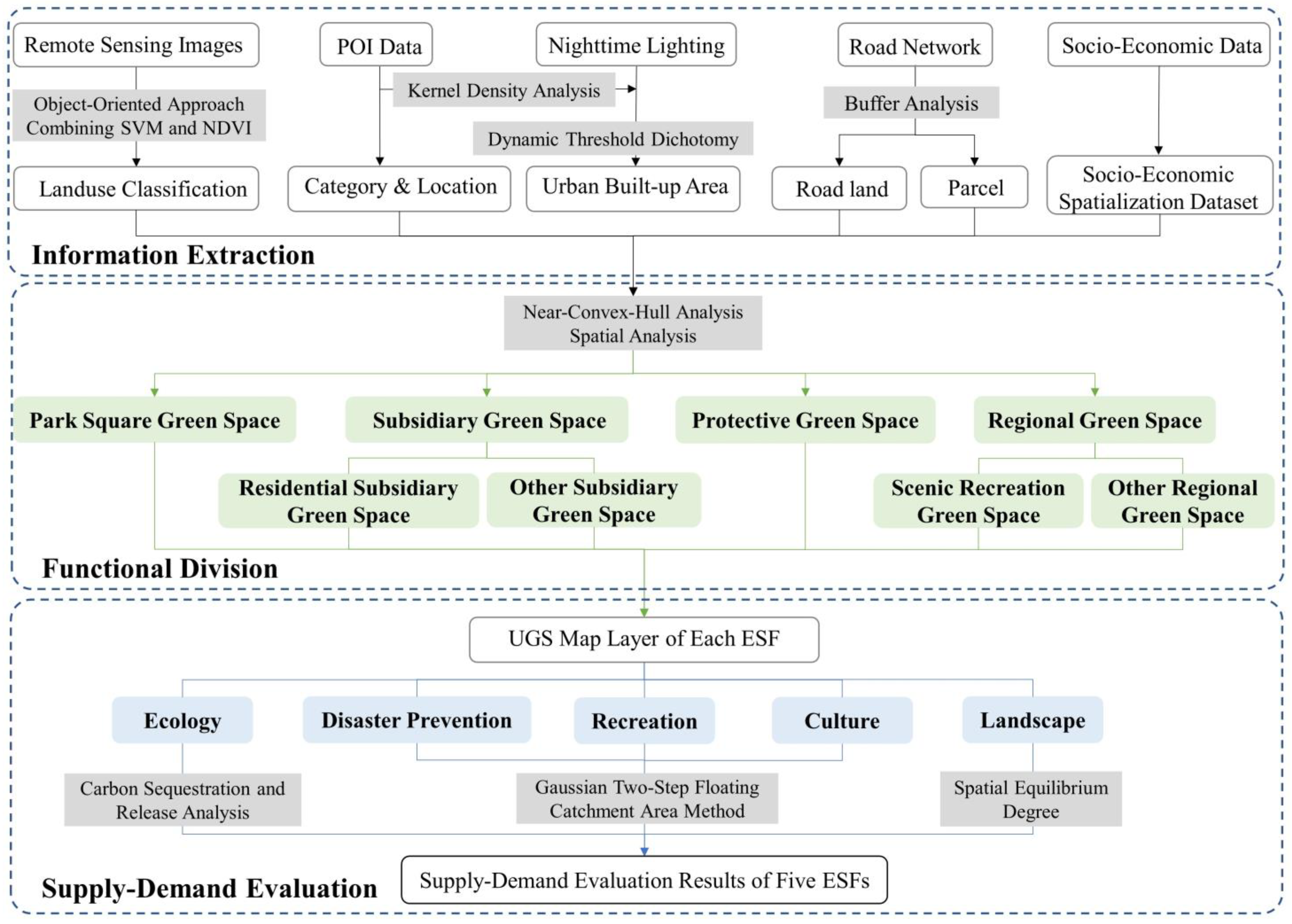
This study established a detailed workflow for evaluating the ESF supply–demand status of UGS (Figure 1). The workflow mainly included three parts: information extraction, functional division and supply–demand evaluation.
In the first part, six information layers were extracted from five multi-source data. Land use types were classified from GF-1 remote sensing images obtained from the China Centre for Resources Satellite Data and Application using an object-oriented approach combining SVM and NDVI. The types and location characteristics of POI data obtained from the Gaode Map were filtered out, and the kernel density of POI was analyzed. Then, combined with the night-time lighting data which was obtained from the National Earth System Science Data Center, National Science & Technology Infra-structure of China, the urban built-up area was extracted using dynamic threshold dichotomy. The road land was obtained through buffer analysis in grades of the road network obtained from OpenStreetMap, and then the parcels were separated out. Socio-economic data obtained from the Resource and Environment Science and Data Center of the Chinese Academy of Sciences was processed into socio-economic spatialization dataset combined with parcels.
In the second part, by fusing the information of multi-source data, six functional types of UGS were classified, including park square green space, residential green space, other subsidiary green space, protective green space, scenic recreation green space, and other regional green space. Near-convex-hull analysis was used to distinguish scenic green space and residential green space. Then, park square green space and scenic recreation green space were separated from scenic green space; other regional green space and other subsidiary green space were separated from other green space; overlay UGS and road land to extract protective green space.
In the third part, five ESFs of UGS, including ecology, landscape, disaster prevention, recreation and culture, were evaluated for supply and demand, respectively. Carbon sequestration and release analysis was used to evaluate ecology; spatial equilibrium degree was used to evaluate landscape; the Gaussian two-step floating catchment area method was used to evaluate disaster prevention, recreation, and culture. Finally, we explored differences in five ESFs for the same UGS and the contribution of UGS functional types for ESF improvement.
2.1. Study Area
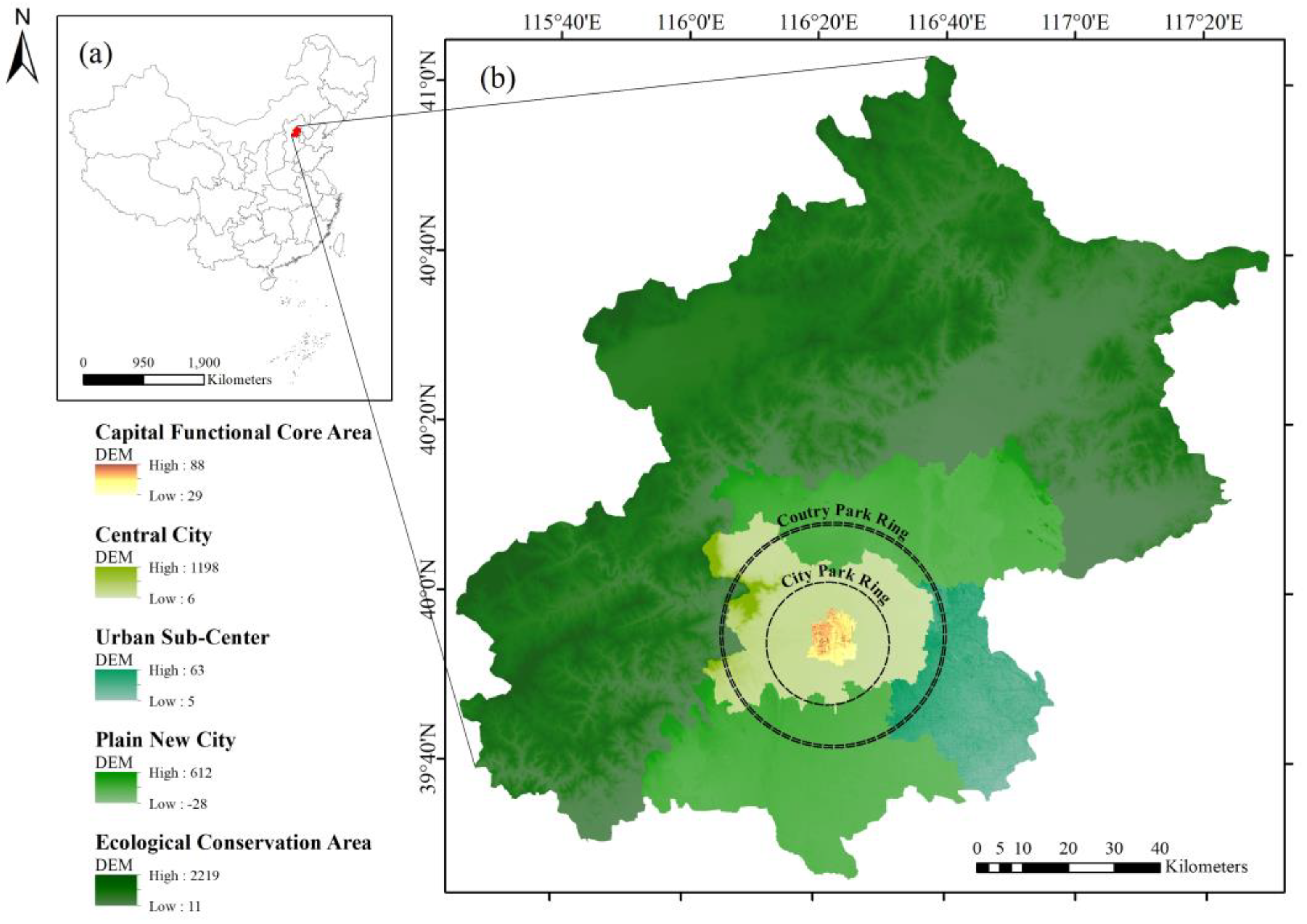
Beijing is located in the northern part of the North China Plain of China [38], as shown in Figure 2a. In the documents officially released by Beijing [39,40,41], five functional areas and two park rings are planned for the construction of UGS (Figure 2b).
The five functional areas include the capital functional core area, the central city, the urban sub-center, the plain new city, and the ecological conservation. The capital functional core area is an important window area to show the image of the national capital, which is proposed to build the second ring cultural landscape ring. The central city, as an important area for the deconstruction of non-capital functions, should also become the core area of green space shortage of deconstruction and supplement through increasing green space and building a greenway system. The goal of the urban sub-center is to build a forest city with blue and green interweaving. Through measures of building large-scale green space and managing abandoned factories, two ecological green belts, a green leisure and recreation ring, and an urban green heart will be formed. The plain new city, as a key area to undertake the appropriate functions of the central city and guarantee the functions of the capital, is planned to form a continuous green ecological space to build ecological conservation areas and leisure areas. As the largest functional area in Beijing, the ecological conservation area is an important ecological barrier for the capital, which should take safeguarding the ecological security of the capital as the main task, building a demonstration area of ecological development that is suitable for living, working and traveling and a model area showing Beijing’s history and culture and beautiful natural landscape.
The two park rings include the urban park ring and the country park ring. The urban park ring is basically located in the fifth ring area, which is a key area to serve and guarantee the ecological security pattern of the central city. The plan proposes that the urban park ring strive to achieve full parkland in 2035. The country park ring extends from beyond the city park ring to outside the sixth ring. This ring is a large-scale green space and strategic space for maintaining the resilience of urban ecological security and consolidating the ecological security pattern of the plain area.
2.2. Data Sources and Processing
- GaoFen-1 remote sensing image data.
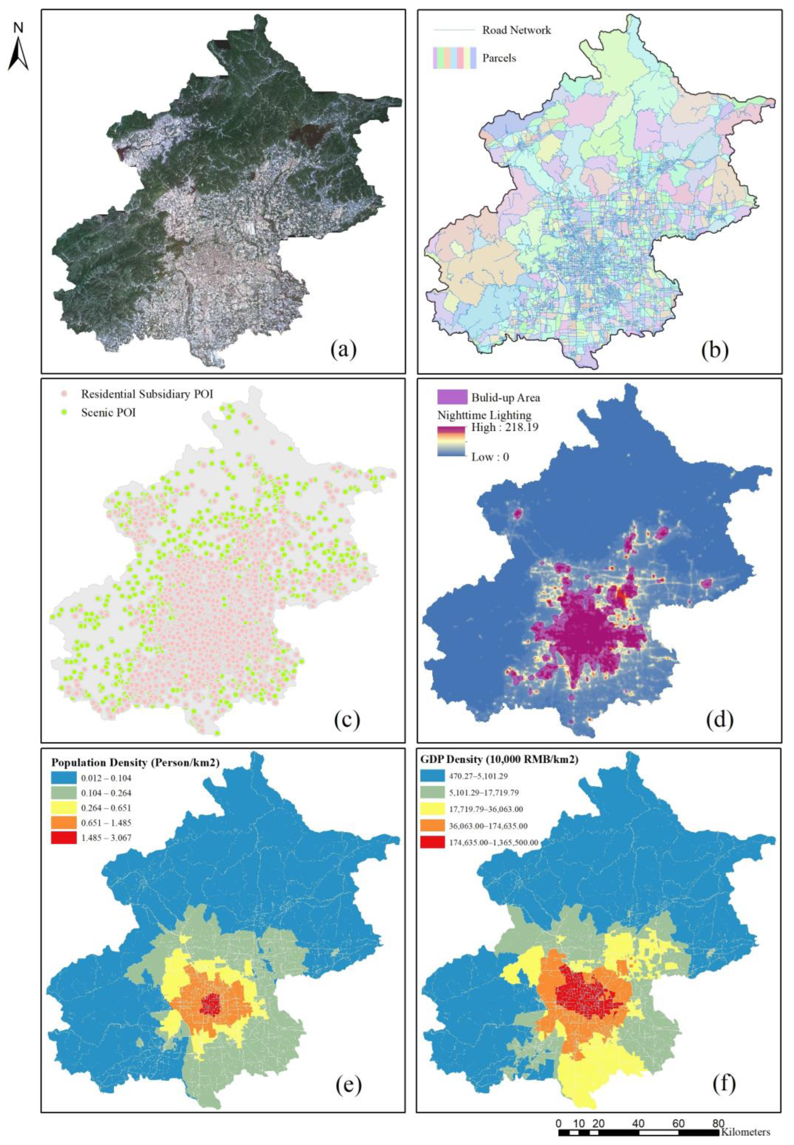
The GaoFen-1 (GF-1) satellite is the first satellite of China’s High Resolution Earth Observation System. We chose to use multispectral image with 4 bands of 16 m spatial resolution. Four images that could cover Beijing on May 27, 2022 were obtained from the China Centre for Resources Satellite Data and Application (https://data.cresda.cn, accessed on 18 August 2022). When the local summer is in full bloom and the vegetation grows, it is conducive to separating UGS from other surrounding features. After acquiring the original image, a series of pre-processing works were carried out with ENVI and ArcGIS software, including radiometric calibration to eliminate errors caused by the sensor itself, FLAASH atmospheric correction to eliminate errors caused by atmospheric scattering and reflection, orthorectification correction to eliminate geometric deformation errors, and alignment with road network data, so as to finally obtain an image that can be used to extract UGS and smoothly integrate with other multi-source data (Figure 3a).
- 2.
- Road network data.
Road network data is mainly used to divide the study area into parcels. As a natural division boundary in urban areas, each parcel has relatively the same type of social function. Dividing the city by parcels can facilitate the functional classification of UGS later. The road network data were obtained from OpenStreetMap (OSM), which has different levels of classification for roads. This study classified five main road types into three levels (Table 1, Figure 3b). 40 m, 20 m, and 10 m buffer radii were established as road space according to Chinese road construction standards and actual road conditions. The road network data were segmented into parcels using the method of Zhang et al. (2017) [42] to finally obtain 6193 parcels in the study area.
- 3.
- Point-of-Interest (POI) data.
Two major categories of scenic and business residential POIs in the study area were obtained through the application programming interface (API) provided by Gaode Map (https://www.amap.com, accessed on 18 August 2022). Then, the POIs of the residential area category were extracted from the business residential. Scenic POIs and residential subsidiary POIs were acquired to participate in the subsequent functional UGS classification work. Finally, a total of 69,488 valid POI data was obtained (Figure 3c).
- 4.
- Nighttime lighting data.
Due to the good coupling relationship between nighttime lighting (NTL) and POI, they are often effectively integrated for the extraction of built-up area [43,44], which is also beneficial to eliminate the effects of nighttime lighting background noise and lighting spillover. In this study, NTL data with a spatial resolution of 500 m in 2020 was obtained from National Earth System Science Data Center, National Science & Technology Infrastructure of China (http://www.geodata.cn, accessed on 18 August 2022). The NTL&POI composite index was used, and the dynamic threshold dichotomy method was selected for the extraction of the built-up area in the study area with reference to the city statistical yearbook data. The specific methods were as follows: (1) Data normalization. The nighttime lighting data and POI kernel density data were normalized to obtain the normalized values , , respectively. (2) Comprehensive index calculation [45]. The positive correlation between the two types of data and the urban built-up area was synthesized using the mean value method, and the calculation formula was as follows.
where, is the integrated index of NTL&POI; is the normalized nighttime light value at point ; is the normalized POI kernel density value at point . (3) Dynamic threshold dichotomy method. According to the built-up area of each city in the statistical yearbook, the dichotomous method was used to continuously change the dynamic threshold value, calculate the dynamic threshold value when it is closest to the area of built-up area, and delineate the scope of built-up area (Figure 3d). Compared with the remote sensing monitoring data of land use status in China obtained from the Resource and Environment Science and Data Center of the Chinese Academy of Sciences (https://www.resdc.cn/, accessed on 18 August 2022), the overlapping proportion of built-up areas reached 84.72%.
- 5.
- Socio-economic data.
Two kinds of kilometer grid datasets of spatial distribution of population and GDP within the study area up to 2020 were obtained from the Resource and Environment Science and Data Center of the Chinese Academy of Sciences (https://www.resdc.cn/, accessed on 18 August 2022). Two datasets were extracted to the study parcels separately to obtain the average values of population and GDP unit area (km2) of each parcel (Figure 3e,f). Socio-economic data such as total energy consumption, total resident population, total annual GDP, and urban built-up area of the study area in 2020 were obtained from the Beijing Municipal Bureau of Statistics “Statistical Yearbook of Various Regions” to provide data support for the ESF supply–demand evaluation in the later section.
2.3. Functional UGS Extraction
2.3.1. Identification of UGS
The object-oriented remote sensing image classification method uses rich spectral, texture, and shape features to classify UGS. Firstly, based on the principle of regional heterogeneity, the remote sensing image is segmented into individual image objects according to the actual feature categories. Then the segmented image objects are used as the smallest classification unit to obtain the feature classification results using a suitable classification algorithm. Compared with the image element-based remote sensing image classification method, the object-oriented method is suitable for high-resolution remote sensing images with rich detail information and large local heterogeneity, which can improve the classification speed as well as the image classification accuracy.
The basic principle of the support vector machine (SVM) algorithm is to find the hyperplane that can optimally solve the classification by exploring the relationship between the training set and the category [46]. In this study, because the water on the acquired images of the study area (especially the water system around the city) had phytoplankton growth, such as green algae, the distinction between water and UGS on remote sensing images using the SVM algorithm alone was not precise enough. So, the normalized vegetation index (NDVI) was introduced to screen UGS again, based on the classification of the SVM algorithm. Overall, our study used an object-oriented green space identification method combining SVM and NDVI to achieve UGS information extraction for Beijing.
2.3.2. Functional Classification of UGS
From the perspective of functional use, UGS can be classified into five major categories: park green space (G1), protective green space (G2), square space (G3), subsidiary green space (XG), and regional green space (EG), according to the Standard for Classification of Urban Green Space (CJJ/T85-2017) of the Ministry of Housing and Urban-Rural Development of the People’s Republic of China [47] (Table 2).
According to the national standard classification and the characteristics of UGS in the study area, park green space and square green space assume roughly the same ESF, and it is difficult to distinguish them when extracting by remote sensing images. Our study collectively referred to park green space and square green space as park square green space. Among the urban subsidiary green space, the residential subsidiary green space is special from other subsidiary green space (such as the subsidiary green space for public management and public service facilities, industrial subsidiary green space, logistics and storage subsidiary green space, etc.), which highlight the special ESF of recreation, so the subsidiary green space was divided into two categories: residential subsidiary green space and other subsidiary green space. In the regional green space, scenic recreation green space is special from other regional green space (such as ecological conservation green space, regional facilities protection green space, production green space, etc.), which highlight the special ESF of recreation and culture, so the regional green space was divided into two categories: scenic recreation green space and other regional green space.
In summary, our study divided four categories of Level I: park square green space, protective green space, subsidiary green space, and regional green space; two categories of Level II under subsidiary green space: residential subsidiary green space and other subsidiary green space; two categories of Level II green space under regional green space: scenic recreation green space and other regional green space (Table 2).
- Classification Based on Near-Convex-Hull Analysis
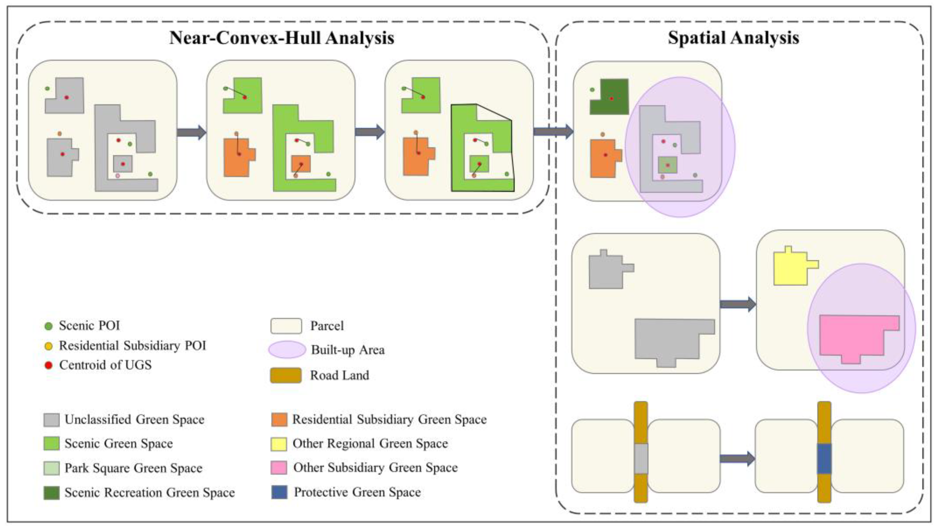
The near-convex-hull analysis was used to distinguish scenic green space and residential subsidiary green space (Figure 4). The method required POI data (including scenic POI and residential subsidiary POI) and UGS patches in each parcel. The analysis process involved two major stages. In the first stage, we selected UGS in the parcel included POI, and then assigned each UGS to the functional attribute of the nearest POI to obtain the initial green space classification result. Although there was the subsidiary POI in the scenic area, all of the UGS in this area should also belong to the scenic green space, referring to the near-convex-hull analysis method proposed by Chen et al. (2018) [48]. So, the second stage was to carry out the correction of the initial results. The convex hull of each UGS (the convex polygon that can connect the outermost points of each UGS and contain the whole UGS) was calculated, to correct UGS which convex hull contains the scenic POI to the scenic green space, and correct the subsidiary green space included in the scenic green space convex hull to scenic green space. Scenic green space was park square green space or scenic recreation green space inside or outside the built-up area of the city, respectively.
- 2.
- Classification Based on Spatial Analysis
The spatial analysis mainly realized the division of park square green space and scenic recreation green space from scenic green space, the division of other regional green space and other subsidiary green space from other green space, and the extraction of protective land through overlay analysis of green space and road land (Figure 4). The specific process is as follows.
According to the definition of park square green space and scenic recreation green space, and on the basis of extracting the built-up area of the city, the scenic green space was overlaid with the built-up area of the city. Located within the built-up area was park square green space, and that which was located outside the built-up area was scenic recreation green space.
Based on the location relationship, UGS in the parcel without POI was screened and classified as other subsidiary green space or other regional green space. Similarly, with the division method of park square green space and scenic recreation green space, other subsidiary green space or other regional green space was divided according to whether it was within the built-up area or not.
According to the definition of protective green space and based on the principle of parcel division, the road buffer area and UGS were overlaid to obtain UGS that does not belong to the parcel, which was called protective green space.
2.3.3. Accuracy Verification
In order to determine the accuracy of UGS extraction and its functional classification, and to ensure that the subsequent evaluation is meaningful, the accuracy of the six functional types of UGS and non-green map layers was verified. According to the method of Yang et al. (2018) [49], 1000 sample points were randomly generated, and then 16 m × 16 m square grids were thus generated as the sample cells. The confusion matrix was obtained by manual interpretation regrading to the latest image and POI data of the Gaode Map and was used to calculate the total accuracy, producer’s accuracy, user’s accuracy and Kappa coefficient.
2.4. ESF Evaluation Method
Our study took the five ESFs of ecology, landscape, disaster prevention, recreation, and culture as the guide [50]. Firstly, categories of functional UGS with various ESF were determined, and then the supply–demand evaluation of five ESFs was finished. Among them, six functional types of UGS have ecology and landscape functions at the same time; park square green space, scenic recreation green space, residential subsidiary green space, other subsidiary green space, and protective green space have disaster prevention function; park square green space, residential subsidiary green space and scenic recreation green space have recreation function; park square green space and scenic recreation green space have culture function. (Table 3).
2.4.1. Ecology
UGS assumes an important role in regulating the carbon and oxygen balance of urban composite ecosystems. Because the carbon cycle is an essential material cycle in human production and life, the study of supply–demand evaluation of carbon sequestration in UGS is representative of ecology function. Therefore, the carbon sequestration and release amount were selected as the index supply–demand evaluation of ecosystem function, to measure the degree of carbon emission generated by human behavior absorbed by the UGS ecosystem. Taking the parcel as the supply–demand evaluation unit, the model of carbon sequestration and release was unified as the amount of CO2.
The supply of ecology function was the carbon sequestration of the UGS ecosystem. Carbon stock was an important parameter to evaluate the carbon sequestration of UGS, referring to the size of the UGS carbon pool under specific spatial, temporal and geographical conditions. Carbon stock was calculated from carbon density and actual green space area, and the carbon density of each functional UGS was derived from the field measurement study by Zhu et al. (2020) [51] (Table 4). The carbon sequestration capacity of each study unit was the sum of the carbon stocks of each functional UGS in the study unit. The specific calculation formula of the supply model was as follows.
where, is the annual carbon sequestration of UGS in the study unit (kg/year); is the annual carbon sequestration of different types of UGS (kg/year); n = 6, representing six functional types of UGS; is the area of each parcel of each functional type of UGS (m2); is the carbon density of each functional type of UGS (kg/m2/year); is the ratio of the amount of substances of CO2 to C.
The demand of ecology function was the carbon emission behavior triggered by urban socio-economic activities, mainly considering human respiration and energy consumption. Among them, energy consumption referred to the sum of all kinds of energy consumed by various industries of the national economy and residential households in a certain period, including various aspects such as energy consumption for living, industrial energy consumption and transportation energy consumption. The number of population in each evaluation unit was calculated from the spatialization dataset of population; the total energy consumption was calculated by establishing a relationship model with the spatialization data of GDP. The demand model [52] was calculated as follows.
where is the annual carbon emission from the study unit (kg/year); is the total carbon emission from the population breathing in the study unit per year (kg/year); is the carbon emission from breathing per person per day 0.9 kg/person/day; is the total population of the study unit (person); is the total carbon emission from the energy consumption in the study unit per year (kg/year); is the converted standard coal amount of the total energy consumption of the study unit (kg/year); is the carbon content of standard coal (80.99%); is the ratio of CO2 to the amount of C.
After calculating the amount of carbon sequestration and release by each evaluation unit, the ecology function supply–demand evaluation coefficient C was constructed to characterize the ecology function state of UGS. The calculation model was as follows.
2.4.2. Landscape
As an important part of the urban landscape, the spatial distribution of UGS is one of the important indicators for evaluating the fairness of landscape patterns. The spatial equilibrium degree [53] is a quantitative index to evaluate the equilibrium of UGS patch distribution from the perspective of social individuals. Our study introduced spatial equilibrium degree for landscape function supply–demand evaluation of UGS.
The spatial equilibrium degree mainly measures the ratio of UGS coverage within the neighborhood. The average ratio of UGS in the study area is used as a benchmark to evaluate the spatial distribution equilibrium in a specific range. According to Guiding Opinions on Promoting the Healthy Development of Urban Landscaping of the Ministry of Housing and Urban-Rural Development of China [54], the development requirement of UGS is “300 m to see green, 500 m to see garden”, so the radius of the neighborhood was defined as 500 m, which was calculated as follows.
where, is the area of UGS contained in the neighborhood range; is the total area of the neighborhood range; is the area of UGS contained in the study area; is the total area of the study area.
After obtaining the landscape equilibrium value within each image element, taking the parcel as the evaluation unit, the mean value of the landscape equilibrium value of the image element within the evaluation unit was calculated, to obtain the calculation result of the landscape equilibrium of each evaluation unit.
2.4.3. Disaster Prevention, Recreation and Culture
The disaster prevention function is mainly reflected when a fire, earthquake, or other man-made or natural disaster happens; reaching the refuge in the shortest time can effectively reduce unnecessary casualties through effective evacuation. Recreation and culture functions play an important role in enhancing the entertainment richness of residents and creating a more comfortable living environment. Recreation function refers to UGS serving the residents’ conditions for a short distance of relaxation and leisure to improve their physiological and psychological health. Culture function refers to UGS serving the residents’ conditions for a long time out, which also plays a role in enhancing the aesthetic perception and ideological insight on the basis of relaxing the body and mind. The three ESFs mainly measure the timeliness of the demand point to the supply point, so spatial accessibility, which can evaluate the spatial difficulty of getting from the demand point to the facility point within a certain time, was used to evaluate these three ESFs supply–demand status.
Not only the distance cost between demand and supply points is the key in spatial accessibility analysis, but also the matching status of supply and demand is an important aspect of measuring the supply–demand status. Using the idea of spatial decomposition, Luo et al. (2003) [55] improved and named the two-step floating catchment area method, which, respectively, formed a search domain as a spatial unit for demand and supply points to improve the measurement method of the interaction between service space supply and population demand. Considering that the interaction between demand and supply points decreased with the increase of distance, a Gaussian distance decay function was introduced [56], on a basis which was suitable for the accessibility study of these three functions. The Gaussian two-step floating catchment area method was divided into two steps.
In the first step, the spatial distance was set from the supply point; next, the OD cost matrix was used to form the spatial search scope of the supply point, and then the number of demanders falling in the demand point within the scope was calculated. The distance decay weight was assigned, and the weighted number of demanders was accumulated, respectively, to obtain the number of potential demanders at each supply point. Finally, the supply area of the supply point was divided by the number of demanders at the demand point to obtain the supply-to-demand ratio within the search scope of the supply point.
where is the supply capacity of UGS ; is the spatial distance from the center of parcel to the center of UGS ; is the population of parcel in the spatial area of UGS ; and is the Gaussian function that introduces the spatial frictional effect, which was calculated as follows:
In the second step, the spatial distance was set from the demand point to form its spatial search scope. Next, the supply–demand ratios of the supply points falling within the scope were given distance decay weights, and then the weighted supply–demand ratios were summed, to obtain the spatial accessibility from the demand point to the supply point.
where, is the per capita possession of UGS in the spatial search domain of parcel , which is the UGS accessibility of each parcel; is the ratio of supply–demand of supply point in the search role domain of parcel .
For the setting of spatial distance, 1000 m, 2500 m and 10 km were taken as the spatial distances for calculating the accessibility of disaster prevention, recreation and culture function, respectively.
3. Results
3.1. Accuracy Verification of Functional UGS Classification Result
The overall classification accuracy was 81.90%, and the Kappa coefficient was 0.78 (Table 5). The overall classification could meet subsequent supply and demand evaluation requirements. The accuracy of the other subsidiary green space was the lowest, and it was easily misclassified as residential subsidiary green space or protective green space, which may be related to the lack of accurate classification conditions and the small size of UGS that were not easily identified. There were more confusions between park square green space and residential subsidiary green space, mainly because it was not easy to define the type of UGS in the community parks near residential areas. In suburban areas, residential subsidiary green space, scenic recreation green space, and other regional green space were easily confused with cultivated land in non-green space. In addition to the reason that the classification method needed to be more precise, it was also related to the fact that UGS in rural areas were functionally integrated and mostly non-monotypic.
3.2. Spatial Distribution Pattern of Functional UGS
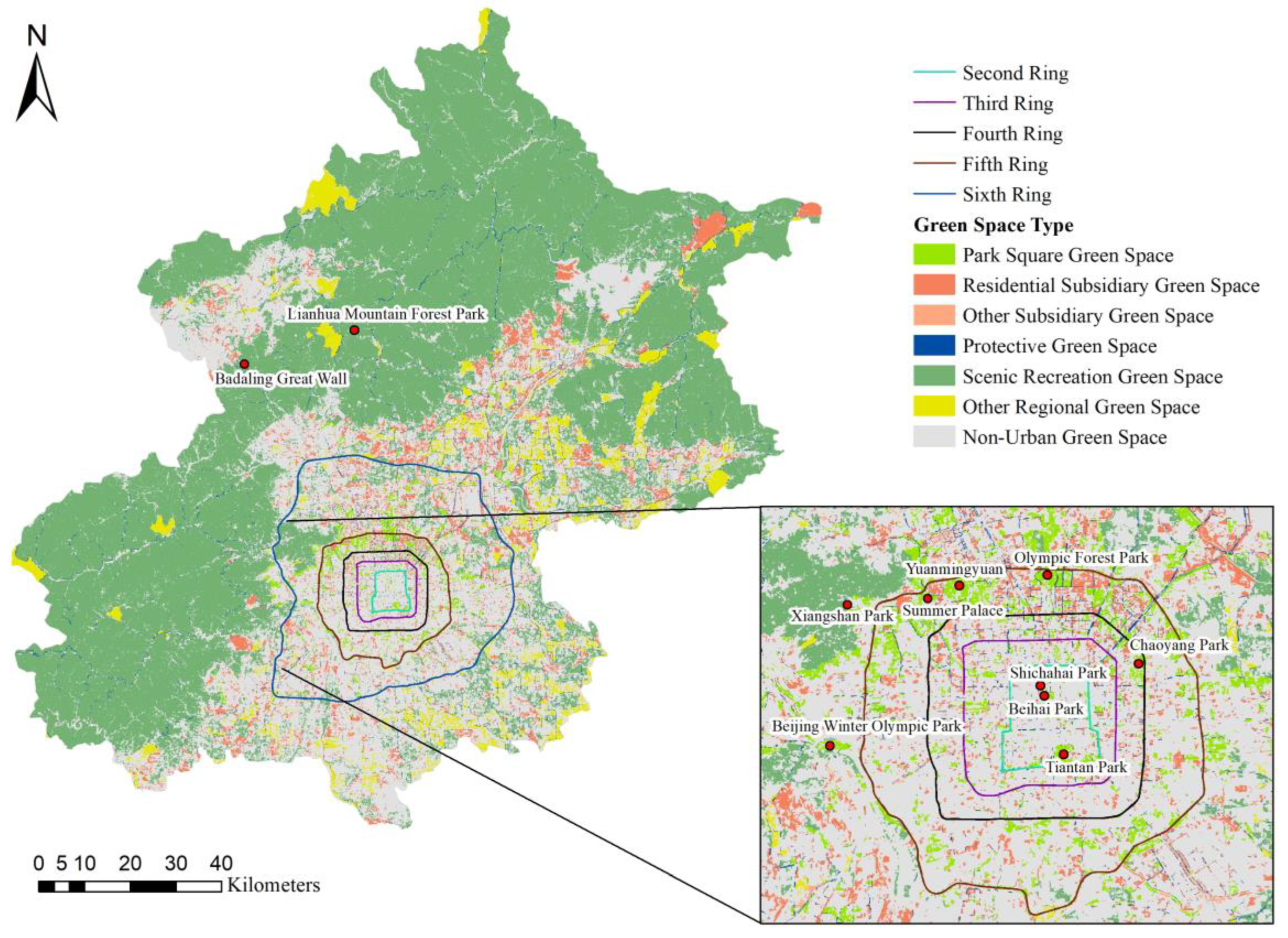
Overall, the area of UGS in Beijing accounted for 65.65%. In terms of the spatial distribution pattern, the UGS characteristic was clearly sparse in the central area and dense in the external area in Beijing, which was inversely consistent with the spatial distribution pattern of the city’s developed intensity. The distribution of UGS within the fourth ring was sparse and the patch size was small. The density of UGS increased significantly between the fourth ring and sixth ring, especially in the northern fifth ring. Outside the sixth ring, due to the presence of the Taihang Mountains in the western and northern areas, the natural green space coverage was high. Large areas of mountains with good ecological conditions could play an important role in improving the UGS coverage ratio of the city. The UGS distribution in eastern and southern areas with the flat terrain was sparser than the western and northern areas because of cultivated land as the main land use type.
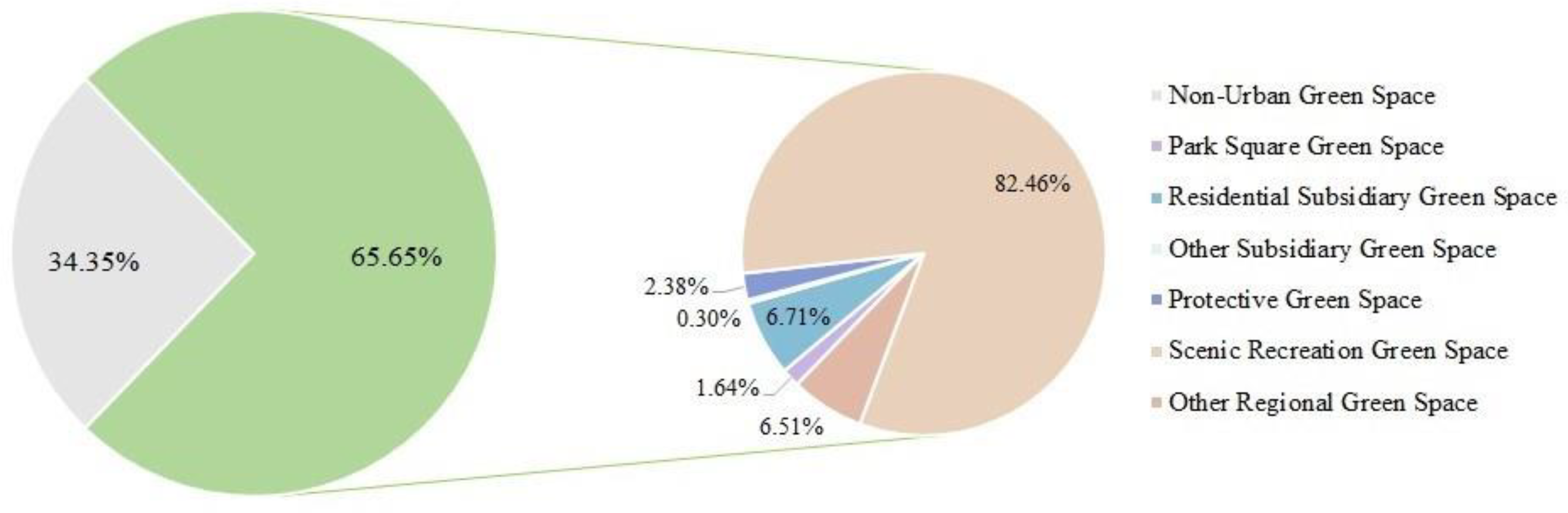
The distribution and area share of functional UGS were shown in Figure 5 and Figure 6. Park square green spaces accounted for 1.64% of UGS, mainly distributed within the sixth ring, and they were mostly large green space patches. For example, there were Beihai Park, Tiantan Park and Shichahai Park near the center of the city, and large scenic parks such as Olympic Forest Park, Summer Palace and Beijing Winter Olympic Park near the periphery of the built-up area. A total of 6.71% of the residential subsidiary green spaces were distributed throughout the study area, except for the western and northern mountainous areas. As an essential part of the residential environment, the area of residential subsidiary green space was the second largest among the functional UGS. With the trend of moving residential areas to the outside of the city, residential subsidiary green spaces were more densely distributed near the urban built-up area boundary than the urban center. The proportion of other subsidiary green space was the lowest at 0.30%, mostly distributed around the residential green spaces as a supplement to their functions. The percentage of protective green spaces was 2.38%, and the distribution pattern could show the developed traffic distribution in Beijing. The more developed the area, the denser the distribution of highways and major roads in the city, the more UGS on both sides of the roads would be distributed, so the area of protective green space would be increased. Scenic recreation green spaces, the most dominant functional UGS in Beijing, accounted for 82.46%. With the mountain areas in the west and north being reasonably developed as scenic recreation sites, such as Xiangshan Park, Badaling Great Wall and Lianhua Mountain Forest Park, the scenic recreation green spaces had been fully developed. Other regional green spaces, accounting for 6.51%, were distributed mainly in the east and south, and consistent with the distribution of cultivated land to some extent. Other regional green spaces mainly contain ecological conservation green areas, production green areas, etc. Therefore, other regional green spaces were mainly distributed outside the built-up areas of the city and were characterized by a large contiguous distribution.
3.3. Supply–Demand Evaluation Result of ESFs
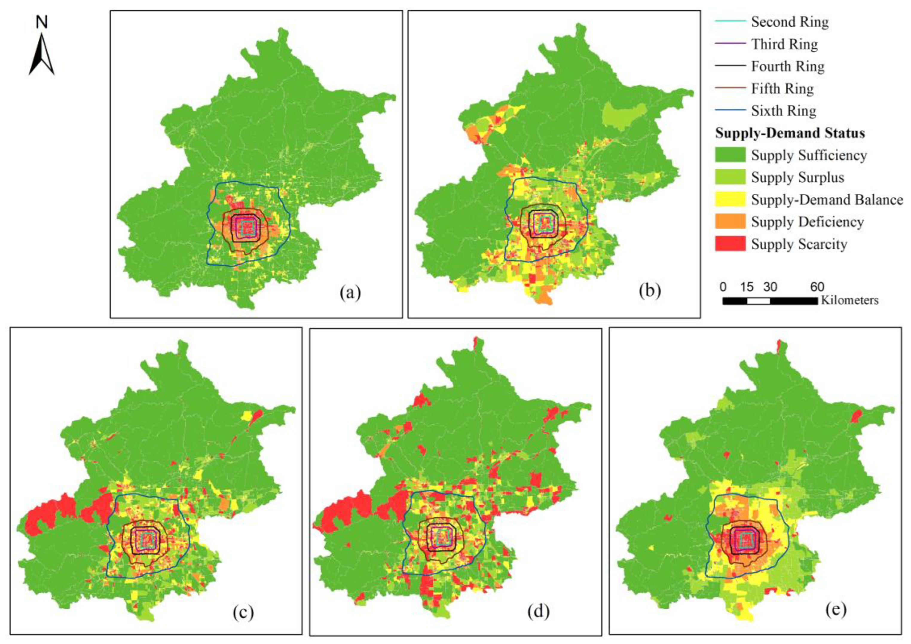
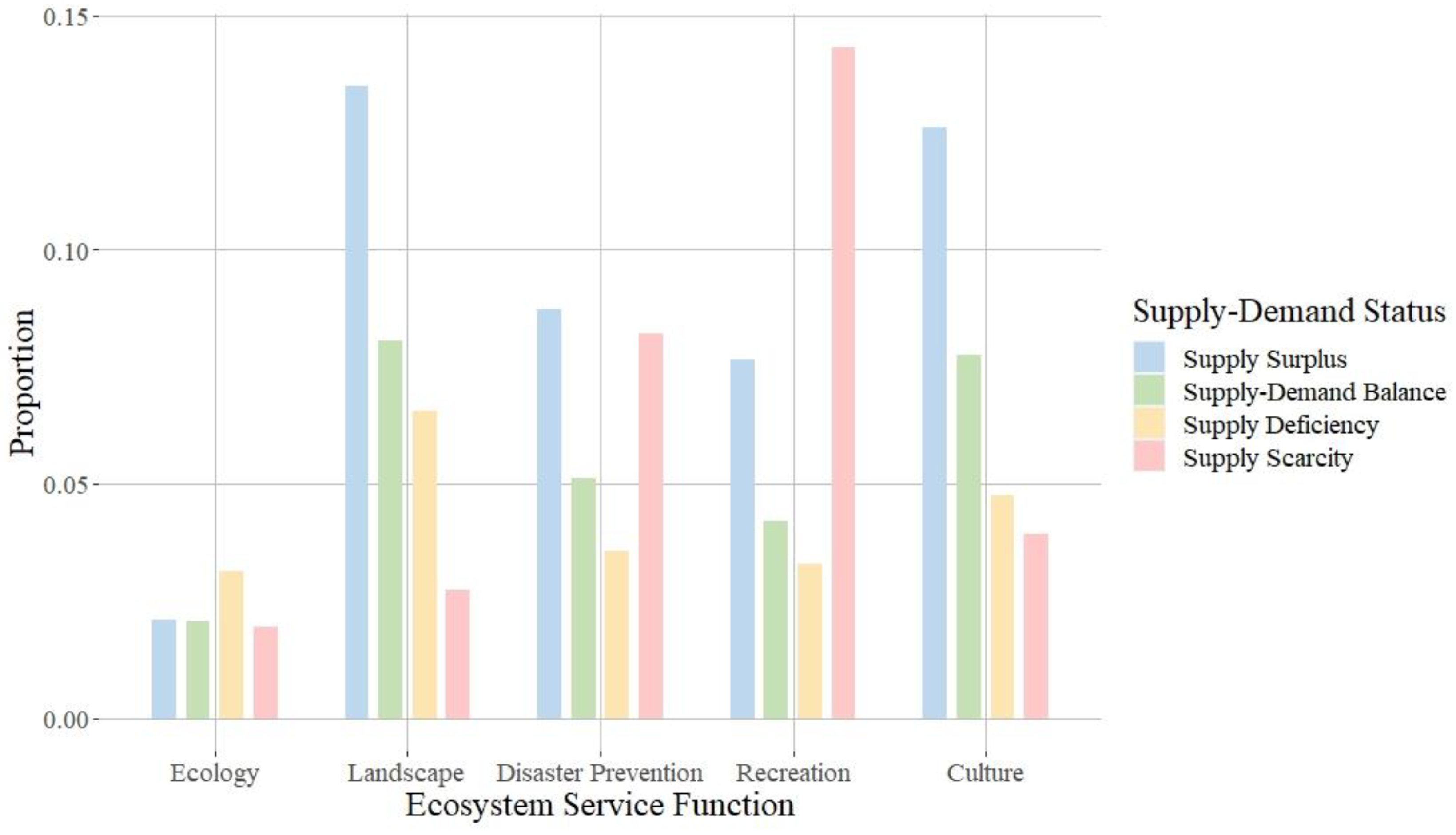
The supply–demand evaluation results of each ESF in the study area were obtained based on the supply–demand evaluation methods, using the parcel as the smallest study unit. The calculated results were classified into supply scarcity, supply deficiency, supply–demand balance, supply surplus and supply sufficiency using the quantile classification method (Figure 7). The proportion of each category not reaching the status of supply sufficiency was shown in Figure 8.
The overall supply–demand state of ecology function in the study area gradually improved from the inside to the outside, with 1.95% and 3.13% of the areas with supply scarcity and supply deficiency, respectively. A total of 94.92% of the area can reach a supply–demand balance or even supply surplus and supply sufficiency. The status of supply scarcity was mainly concentrated in the fourth ring, and the status of supply deficiency was mainly concentrated between the third ring and the fifth ring, which were mainly related to the tight land supply and large population in the city center. The few parcels within the fifth ring that had supply–demand balance or above were due to the distribution of large parks such as Olympic Forest Park, Yuanmingyuan, Chaoyang Park, etc., which had a high level of ecological supply due to large UGS and vegetation coverage. The fact that almost all the areas outside the sixth ring were in supply–demand balance or above was not only related to the fact that the study area was located in a mountainous area with lush natural vegetation but also closely related to the reduction of the population outside the city, relief of land tension and proper planning.
- 2.
The supply–demand state of landscape function in the study area was significantly less than the ecology function, with 2.75% and 6.56% of supply scarcity and supply deficiency areas, respectively. A total of 90.67% of the areas reached supply–demand balance state or above. This indicator mainly measured the size and fragmentation of UGS: the supply–demand state of landscape function in mountainous areas with large areas of natural vegetation distribution was obviously better, and the supply–demand state of landscape function in areas with intensive human activities and large construction land areas was worse. Specifically, the central area was economically developed and had a shortage of land, resulting in less green space and high fragmentation; because of the distribution of more villages and cultivated land in eastern and southern areas, the proportion of UGS was not as high as the northwestern areas, and areas of supply scarcity and supply deficiency were distributed in pieces, which was not conducive to the improvement of landscape supply capacity and the construction of the overall landscape balance of the city.
- 3.
From the supply–demand evaluation result of the disaster prevention function, there were 11.76% of areas where the supply–demand effect in the supply scarcity or supply deficiency state was unsatisfactory; there were more than 85% areas in the supply–demand balance or better state. Supply scarcity and supply deficiency areas were mainly distributed in the city center and suburban rural areas. The demand for disaster prevention was high in the urban center because of the high population density, but the land use type in urban areas was mainly construction land, which provided limited UGS for disaster prevention and avoidance. In rural areas, except for residential construction land, the main land use type was cultivated land, therefore the distribution of UGS for disaster prevention was low. However, under special circumstances, cultivated land could also be used for disaster prevention and avoidance. In general, the actual situation of disaster prevention in suburban areas was better than the calculation results of this study.
- 4.
Compared with the other four ESFs, the supply scarcity areas of recreation accounted for the largest proportion, 14.31%. Due to the high population density and the small number of UGS in the city center, it was not easy to meet the demand for recreation of the large urban population. However, around the large parks and squares within the fifth ring, such as Olympic Forest Park, Tiantan Park, and Chaoyang Park, there were still areas with supply–demand balance or even supply surplus, indicating that the large green space patches in urban centers were very useful in relieving a large amount of recreation demand of urban residents. Rural areas in the suburb also had several supply scarcity areas, indicating that the construction of park square green spaces and residential subsidiary green spaces in rural areas was not enough to fully meet the needs of residents’ recreation.
- 5.
The supply–demand evaluation of culture function showed that, because the search distance had increased to 10 km, large UGS in the suburb were fully utilized to provide culture function. The tight supply–demand situation was gradually relieved from the city center outward, showing a very obvious ring-shaped feature. More than 90% of the areas were in a state where the supply met the demand, which could meet residents’ demand for long-distance trips. However, almost all areas within the fourth ring were in a state of supply scarcity, and there were many areas of supply deficiency between the fourth and sixth ring. Overall, the proportion of supply deficiency areas reached 4.74% and supply scarcity reached 3.94%. The poor supply–demand situation of culture function in the city center showed that even increasing the threshold setting of travel distance could not alleviate the tight supply of UGS to a greater extent because of the scarcity of UGS.
Overall, the accessibility analysis of disaster prevention, recreation, and culture function showed that, in addition to the scarcity of UGS in the region itself, the high population density in the city center, the limited service area of UGS, and the lack ESF of UGS were also important reasons for the bad supply–demand status.
4. Discussion
4.1. Differences in Five ESFs for the Same UGS
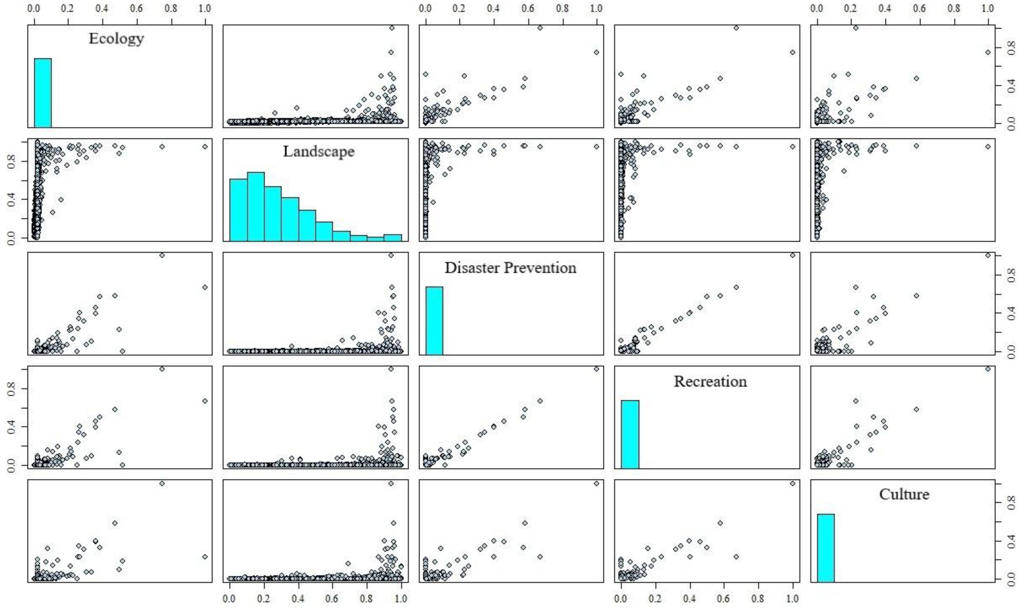
Although there are many studies on evaluating EFS of UGS, it is common to recognize UGS as undifferentiated for relevant research. However, it is undeniable that different functional types of UGS play different roles in ES, which is a blank area of research so far. As the scatter parcel (Figure 9) shows, there was no significant two-by-two correlation between the five functions, indicating that the same parcel of UGS had different degrees of influence in different ESFs. For example, the protective green space on both sides of the road could not assume the same recreation function as the park square green space; scenic recreation green spaces in the suburb do not provide short-distance recreation service for residents living in the urban center; and so on. In this study, the ESFs undertaken by different green space patches were separately determined by using the functional characteristics of UGS. Therefore, a different ES supply–demand situation of UGS was obtained from a new perspective.
4.2. Contribution of UGS Functional Types for ESF Improvement
The division of functional UGS is a comprehensive consideration of the multiple characteristics, according to their location, social roles, and so on. In addition, there are differences in the ESF undertaken by different functional UGS, so the contribution of functional UGS in each ESF is different. For example, the contribution of functional UGS in ecology function is determined by the carbon density of functional UGS, and by contrast, the park square green space has the largest contribution per unit area; for the culture function, it is provided by park square green space in built-up areas and by scenic recreation green space outside built-up areas. Residents also have preferences for the type of UGS in different life scenarios. For example, during weekdays, people prefer to spend time in residential subsidiary green spaces close to their homes, and during holidays, they prefer to travel to larger parks. Therefore, when building UGS, if there is a planning purpose of enhancing the specific ESF of a specific area, it can be traced to what kind of functional UGS should be built, which is a new idea to enhance the service capacity of UGS suiting local conditions.
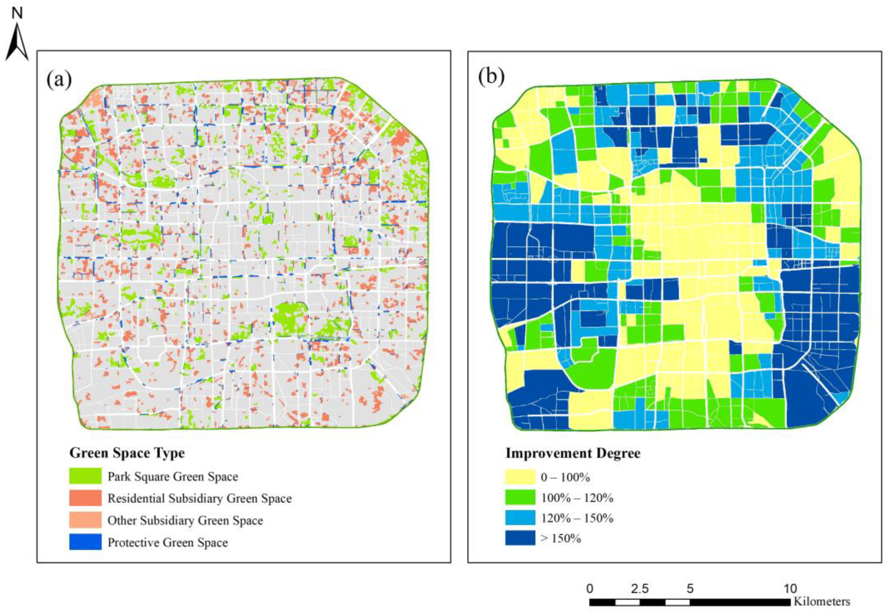
We specifically explored how much change would be brought to the supply–demand situation if we change the functional type or increase the ESF of existing UGS without changing the existing area. Taking the culture function as an example, it can be seen that almost all UGS within the fourth ring were in a state of supply scarcity (Figure 7e), and there were a large number of subsidiary green spaces which could not provide culture function (Figure 10a). Assuming that these UGS have the same culture service function as the park square green space, we calculated the improvement degree in the supply–demand situation within the fourth ring. A total of 31.84% of the areas had an improvement in the culture service situation within 100%, 19.95% had an improvement of 100–120%, 19.25% had an improvement of 120–150%, and 28.97% had an improvement of more than 150% (Figure 10b). It fully indicates that when the construction area of UGS in the urban center is limited, increasing the high-quality of UGS [57] can greatly improve the ESF supply–demand status.
4.3. Contributions of ES Supply–Demand Status for Beijing Urban Planning and Space Ecological Restoration
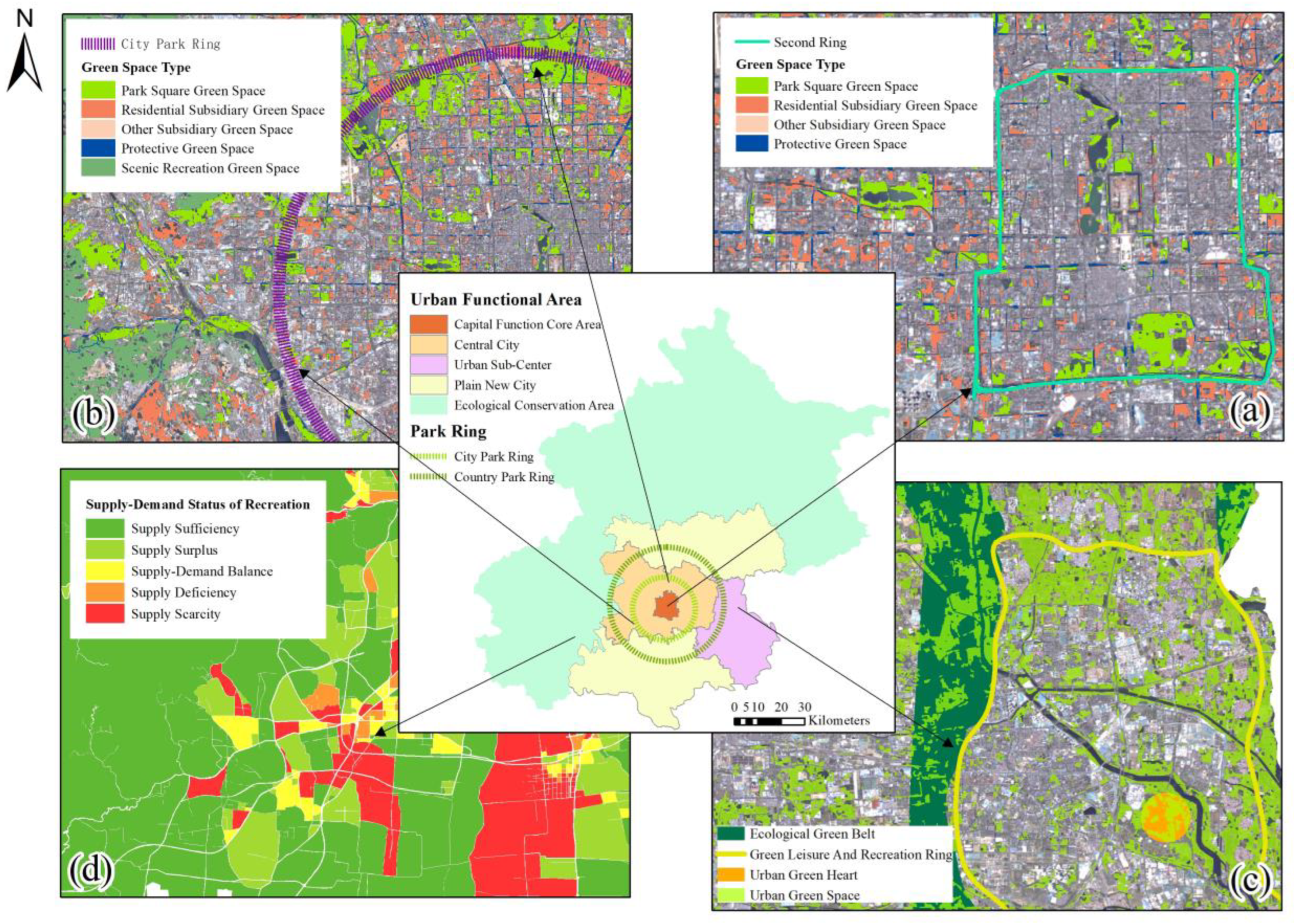
The capital functional core area mainly highlights the landscape and culture functions of UGS, and should pay attention to the construction of subsidiary green space and park square green space, which is proposed to build the second ring cultural landscape ring (Figure 11a). As an important area for the deconstruction of non-capital functions, the central city should pay attention to the construction of UGS with recreation functions, such as park square green space and residential subsidiary green space. Compared with the capital functional core area, our results showed that the supply–demand situation of the recreation function had been significantly improved in this area. Especially in the northeast area, there were large areas of parks square green space and residential subsidiary green space, as well as a large-scale ecological environment construction demonstration area taking shape (Figure 11b).
The goal of the urban sub-center is to form two ecological green belts, a green leisure and recreation ring, and an urban green heart. It can be seen from the supply–demand situation of landscape and recreation functions that there were still some areas where the construction of UGS needed to meet the planning requirements (Figure 11c). The plain new city is proposed to build a continuous green ecological space to build ecological conservation areas and leisure areas. Increasing the proportion of other regional green space and scenic recreation green space is one way to improve the level of ecology, landscape and recreation services. The ecological conservation area is an important ecological barrier for the capital. Therefore, the construction of UGS in this region should be the top priority of regional development. According to the results of our study, strengthening the spatial interaction between UGS and residents in a small part of the western region is necessary to improve the cross-regional utilization of UGS (Figure 11d).
The urban park ring is located in the fifth ring area, which is a key area to serve and guarantee the ecological security pattern of the central city. Our results showed that the northern and eastern areas had a dense distribution of UGS and park coverage. The construction of park square green space in the southwestern area needs to be enhanced to guarantee the construction of the spatial pattern of the central city (Figure 11b). The country park ring extends from beyond the city park ring to outside the sixth ring. As our results shown, the internal supply–demand situation of this ring decreased significantly compared with the external one. Therefore, in the future, the construction of the country park ring should be strengthened as an important way to improve the ES capacity of UGS in the central city.
4.4. The Advantage of Evaluating UGS from Functional and Supply–Demand Perspective
Facing the challenges of evaluating the ESF of UGS, we have achieved progress, whether regarding classification or evaluation. The differences between our study and existing studies are summarized as follows.
Through upgrading the method [48], studying part of Beijing and the category system of UGS, our study realized automatic classification of functional UGS suitable for a large scale of Beijing. Existing studies only focused on the physical features of UGS [58,59], or artificially distinguished social functions of UGS [60]. Such UGS classification approaches are too single and inefficient. The accuracy verification result of functional UGS classification in our study showed good effect of our approach in large scale application, which provides a great idea for classifying functional UGS rapidly and widely in the future.
Our work focused on a completely different aspect of evaluating ESF of UGS. Millenium ecosystem assessment (MA) divided ecosystem services into four types including supporting, provisioning, regulating, and cultural services [9]; common international classification of ecosystem services (CICES) divided ecosystem services into three types including provisioning, regulating and maintenance, and cultural services [61]. Although ESF has been a consistently hot research topic, the studies relating to ESF of UGS were broad and general, rather than showing the unique functions of UGS and the integration of supply and demand. However, a suitable evaluating system which can directly reflect the reality is a key of guiding UGS construction and governmental decision-making. In our study, complete evaluating results of five ESFs of functional UGS in Beijing were generated, which reflected the real supply–demand status of UGS from a social functional aspect. Therefore, our work is meaningful in providing a new research perspective and assisting in evaluating ESF of UGS.
4.5. Limitations and Prospects
First, the division of functional UGS has complexity. Because of the complex spatial structure of the city, some UGS have the characteristics of multiple functional complexes. For example, the UGS in the university campus that can satisfy the visiting and gathering activity has the attributes of both park square green space and residential subsidiary green space. The functional types of UGS were only classified as the most significant categories. Combined with the limitation of remote sensing image resolution and the unreliable situation of some social perception data, more data is needed to achieve a reasonable classification of UGS with compound functions. In future research, to identify more functional types of UGS and improve classification accuracy, higher resolution remote sensing data (aerial photography) and LiDAR data will be considered, the automatic processing capability of data and the text analysis capability of POI data will be improved, and more rigorous and comprehensive feature identification will be carried out.
Second, ESs are not provided by green space ecosystem alone in the city. Other ecosystems may have an overlap with the green space ecosystem, but it is not easy to measure the proportion of different ecosystem supplies. For example, the water ecosystem also has a landscape service function, and the joint action with green space ecosystem can enhance the service capacity. When the role of other ecosystems is considered in the future, more complete results could be obtained than this study. Considering the supply capacity of various ecosystems together and comparing with the demand may lead to a more realistic result.
5. Conclusions
This paper explored the relationship between the supply and the demand of different ESFs from the perspective of UGS functions. Compared to existing research, our work had four unique points: (1) The automatic extraction technique of functional UGS integrating multi-source data was feasible, both in terms of extraction accuracy and practical significance. (2) Sorting out the contribution provided by each functional UGS for ESF can measure the performance of the same UGS in different ESFs, which was a necessary prerequisite for the precision construction of UGS. (3) The supply–demand evaluation results obtained by considering both supply and demand in the same dimension were more intuitive to see whether the city’s demand for UGS has been met, compared to single-side evaluation. (4) From the research results of Beijing, it can be seen that the spatial distribution density of UGS was negatively related to the degree of regional development, and the contribution of the same parcel of UGS in five ESFs was different. The ES supply–demand status in Beijing could assist government departments in urban planning and space ecological restoration. In future work, more rigorous and comprehensive feature identification will be conducted to solve the classification problem of compound functions of UGS. In addition, the contributions of other ecosystems besides UGS in ESF supply–demand evaluation will be considered.
Author Contributions
Conceptualization, Y.W. and H.H.; methodology, Y.W., H.H. and G.Y.; formal analysis, Y.W.; investigation, Y.W.; writing—original draft preparation, Y.W.; writing—review and editing, H.H., G.Y. and W.C.; visualization, Y.W.; supervision, H.H. All authors have read and agreed to the published version of the manuscript.
Funding
This research was funded by National Key R&D Program of China (2017YFB0503800).
Conflicts of Interest
The authors declare no conflict of interest.
References
- Wolch, J.R.; Byrne, J.; Newell, J.P. Urban green space, public health, and environmental justice: The Challenge of making cities ‘just green enough’. Landsc. Urban Plan. 2014, 125, 234–244. [Google Scholar] [CrossRef] [Green Version]
- Derkzen, M.L.; van Teeffelen, A.J.A.; Verburg, P.H. Review: Quantifying urban ecosystem services based on high-resolution data of urban green space: An assessment for Rotterdam, the Netherlands. J. Appl. Ecol. 2015, 52, 1020–1032. [Google Scholar] [CrossRef]
- Lepczyk, C.A.; Aronson, M.F.J.; Evans, K.L.; Goddard, M.A.; Lerman, S.B.; MacIvor, J.S. Biodiversity in the city: Fundamental questions for understanding the ecology of urban green spaces for biodiversity conservation. BioScience 2017, 67, 799–807. [Google Scholar] [CrossRef] [Green Version]
- Aram, F.; Higueras García, E.; Solgi, E.; Mansournia, S. Urban green space cooling effect in cities. Heliyon 2019, 5, e01339. [Google Scholar] [CrossRef] [Green Version]
- Selmi, W.; Weber, C.; Rivière, E.; Blond, N.; Mehdi, L.; Nowak, D. Air pollution removal by trees in public green spaces in Strasbourg City, France. Urban For. Urban Green. 2016, 17, 192–201. [Google Scholar] [CrossRef] [Green Version]
- Kondo, M.C.; Fluehr, J.M.; McKeon, T.; Branas, C.C. Urban green space and its impact on human health. Int. J. Environ. Res. Public Health 2018, 15, 445. [Google Scholar] [CrossRef] [Green Version]
- Kwon, O.-H.; Hong, I.; Yang, J.; Wohn, D.Y.; Jung, W.-S.; Cha, M. Urban green space and happiness in developed countries. EPJ Data Sci. 2021, 10, 28. [Google Scholar] [CrossRef]
- Costanza, R.; d’Arge, R.; de Groot, R.; Farber, S.; Grasso, M.; Hannon, B.; Limburg, K.; Naeem, S.; O’Neill, R.V.; Paruelo, J.; et al. The value of the world’s ecosystem services and natural capital. Nature 1997, 387, 253–260. [Google Scholar] [CrossRef]
- Millenium Ecosystem Assessment. Millenium Ecosystem Assessment Synthesis Report; Island Press: Washington, DC, USA, 2005. [Google Scholar]
- Liu, O.Y.; Russo, A. Assessing the Contribution of urban green spaces in green infrastructure strategy planning for urban ecosystem conditions and services. Sustain. Cities Soc. 2021, 68, 102772. [Google Scholar] [CrossRef]
- Zhou, Y.; Chen, M.; Tang, Z.; Mei, Z. Urbanization, land use change, and carbon emissions: Quantitative assessments for city-level carbon emissions in Beijing-Tianjin-Hebei Region. Sustain. Cities Soc. 2021, 66, 102701. [Google Scholar] [CrossRef]
- Xiao, H.; He, X.; Wang, Y.; Wang, J.; Jiang, Q. Research progress on the correlation between urban green space and residents’ physical and mental well-being from a perspective of matching ecosystem services supply and demand. Acta Ecol. Sin. 2021, 41, 5045–5053. [Google Scholar] [CrossRef]
- Feyisa, G.L.; Dons, K.; Meilby, H. Efficiency of parks in mitigating urban heat island effect: An example from Addis Ababa. Landsc. Urban Plan. 2014, 123, 87–95. [Google Scholar] [CrossRef]
- Ayala-Azcárraga, C.; Diaz, D.; Zambrano, L. Characteristics of urban parks and their relation to user well-being. Landsc. Urban Plan. 2019, 189, 27–35. [Google Scholar] [CrossRef]
- Masoudi, M.; Tan, P.Y. Multi-year comparison of the effects of spatial pattern of urban green spaces on urban land surface temperature. Landsc. Urban Plan. 2019, 184, 44–58. [Google Scholar] [CrossRef]
- Nesbitt, L.; Meitner, M.J.; Girling, C.; Sheppard, S.R.J.; Lu, Y. Who has access to urban vegetation? A spatial analysis of distributional green equity in 10 US cities. Landsc. Urban Plan. 2019, 181, 51–79. [Google Scholar] [CrossRef]
- Barbierato, E.; Bernetti, I.; Capecchi, I.; Saragosa, C. Integrating remote sensing and street view images to quantify urban forest ecosystem services. Remote Sens. 2020, 12, 329. [Google Scholar] [CrossRef] [Green Version]
- Dang, H.; Li, J. The integration of urban streetscapes provides the possibility to fully quantify the ecological landscape of urban green spaces: A case study of Xi’an City. Ecol. Indic. 2021, 133, 108388. [Google Scholar] [CrossRef]
- Heikinheimo, V.; Tenkanen, H.; Bergroth, C.; Järv, O.; Hiippala, T.; Toivonen, T. Understanding the use of urban green spaces from user-generated geographic information. Landsc. Urban Plan. 2020, 201, 103845. [Google Scholar] [CrossRef]
- Zhu, J.; Lu, H.; Zheng, T.; Rong, Y.; Wang, C.; Zhang, W.; Yan, Y.; Tang, L. Vitality of urban parks and its influencing factors from the perspective of recreational service supply, demand, and spatial links. Int. J. Environ. Res. Public Health 2020, 17, 1615. [Google Scholar] [CrossRef] [Green Version]
- Cao, S.; Du, S.; Yang, S.; Du, S. Functional classification of urban parks based on urban functional zone and crowd-sourced geographical data. ISPRS Int. J. Geo Inf. 2021, 10, 824. [Google Scholar] [CrossRef]
- Liu, Z.; Huang, Q.; Yang, H. Supply-demand spatial patterns of park cultural services in megalopolis area of Shenzhen, China. Ecol. Indic. 2021, 121, 107066. [Google Scholar] [CrossRef]
- Willemen, L.; Verburg, P.H.; Hein, L.; van Mensvoort, M.E.F. Spatial characterization of landscape functions. Landsc. Urban Plan. 2008, 88, 34–43. [Google Scholar] [CrossRef]
- Gómez-Baggethun, E.; Barton, D.N. Classifying and valuing ecosystem services for urban planning. Ecol. Econ. 2013, 86, 235–245. [Google Scholar] [CrossRef]
- Hardaker, A.; Pagella, T.; Rayment, M. Integrated assessment, valuation and mapping of ecosystem services and dis-services from upland land use in Wales. Ecosyst. Serv. 2020, 43, 101098. [Google Scholar] [CrossRef]
- Xie, G.; Zhen, L.; Lu, C.; Xiao, Y.; Chen, C. Expert knowledge based valuation method of ecosystem services in China. J. Nat. Resour. 2008, 5, 911–919. [Google Scholar]
- Tang, L.; Wang, L.; Li, Q.; Zhao, J. A framework designation for the assessment of urban ecological risks. Int. J. Sustain. Dev. World Ecol. 2018, 25, 387–395. [Google Scholar] [CrossRef] [Green Version]
- Liu, Q.; Tian, Y.; Yin, K.; Zhang, F.; Huang, H.; Chen, F. Landscape pattern theoretical optimization of urban green space based on ecosystem service supply and demand. IJGI 2021, 10, 263. [Google Scholar] [CrossRef]
- Kolcsár, R.A.; Csikós, N.; Szilassi, P. Testing the limitations of buffer zones and urban atlas population data in urban green space provision analyses through the case study of Szeged, Hungary. Urban For. Urban Green. 2021, 57, 126942. [Google Scholar] [CrossRef]
- Martín-Turrero, I.; Valiente, R.; Molina-de la Fuente, I.; Bilal, U.; Lazo, M.; Sureda, X. Accessibility and availability of alcohol outlets around schools: An ecological study in the city of Madrid, Spain, according to socioeconomic area-level. Environ. Res. 2022, 204, 112323. [Google Scholar] [CrossRef]
- Huang, H.; Zhang, M.; Yu, K.; Gao, Y.; Liu, J. Construction of complex network of green infrastructure in smart city under spatial differentiation of landscape. Comput. Commun. 2020, 154, 380–389. [Google Scholar] [CrossRef]
- Ye, C.; Hu, L.; Li, M. Urban green space accessibility changes in a high-density city: A case study of Macau from 2010 to 2015. J. Transp. Geogr. 2018, 66, 106–115. [Google Scholar] [CrossRef]
- Wu, J.; Chen, H.; Wang, H.; He, Q.; Zhou, K. Will the opening community policy improve the equity of green accessibility and in what ways?—Response based on a 2-step floating catchment area method and genetic algorithm. J. Clean. Prod. 2020, 263, 121454. [Google Scholar] [CrossRef]
- Wang, F.; Wang, K.; Liu, H. Evaluation and influence factors of spatial accessibility of ecological space recreation service in the Pearl River delta urban agglomeration: A modified two-step floating catchment area method. Acta Ecol. Sin. 2020, 40, 3622–3633. [Google Scholar] [CrossRef]
- Ramyar, R.; Saeedi, S.; Bryant, M.; Davatgar, A.; Mortaz Hedjri, G. Ecosystem Services mapping for green infrastructure planning—The case of Tehran. Sci. Total Environ. 2020, 703, 135466. [Google Scholar] [CrossRef] [PubMed]
- Peng, J.; Yang, Y.; Xie, P.; Liu, Y. Zoning for the construction of green space ecological networks in Guangdong Province based on the supply and demand of ecosystem services. Acta Ecol. Sin. 2017, 37, 4562–4572. [Google Scholar] [CrossRef]
- Chen, Z.; Huang, G. Research progress on the differences and connections between supply and demand of urban green space. Chin. J. Appl. Ecol. 2020, 31, 3925–3934. [Google Scholar] [CrossRef]
- Peng, J.; Tian, L.; Liu, Y.; Zhao, M.; Hu, Y.; Wu, J. Ecosystem services response to urbanization in metropolitan areas: Thresholds identification. Sci. Total Environ. 2017, 607–608, 706–714. [Google Scholar] [CrossRef]
- The People’s Government of Beijing Municipality. Beijing Urban. Master Plan (2016–2035), 7th ed.; China Building Industry Press: Beijing, China, 2017; pp. 1–30. [Google Scholar]
- The People’s Government of Beijing Municipality. Beijing Land and Space Ecological Restoration Plan, 1st ed.; China Building Industry Press: Beijing, China, 2022; pp. 53–62. [Google Scholar]
- Beijing Municipal Ecology and Environment Bureau. Beijing 14th Five-Year Plan for the Construction and Development of Greening Isolated Areas, 1st ed.; China Building Industry Press: Beijing, China, 2021; pp. 5–24. [Google Scholar]
- Zhang, Y.; Li, Q.; Huang, H.; Wu, W.; Du, X.; Wang, H. The combined use of remote sensing and social sensing data in fine-grained urban land use mapping: A case study in Beijing, China. Remote Sens. 2017, 9, 865. [Google Scholar] [CrossRef] [Green Version]
- He, X.; Zhou, C.; Zhang, J.; Yuan, X. Using wavelet transforms to fuse nighttime light data and POI big data to extract urban built-up areas. Remote Sens. 2020, 12, 3887. [Google Scholar] [CrossRef]
- He, X.; Yuan, X.; Zhang, D.; Zhang, R.; Li, M.; Zhou, C. Delineation of urban agglomeration boundary based on multisource big data fusion—A case study of Guangdong–Hong Kong–Macao Greater Bay Area (GBA). Remote Sens. 2021, 13, 1801. [Google Scholar] [CrossRef]
- Li, F.; Yan, Q.; Zou, Y.; Liu, B. Extraction accuracy of urban built-up area based on nighttime light data and POI: A case study of Luojia 1-01 and NPP/VIIRS nighttime light images. Geomat. Inf. Sci. Wuhan Univ. 2021, 46, 825–835. [Google Scholar] [CrossRef]
- Ustuner, M.; Sanli, F.B.; Dixon, B. Application of support vector machines for landuse classification using high-resolution RapidEye images: A sensitivity analysis. Eur. J. Remote Sens. 2015, 48, 403–422. [Google Scholar] [CrossRef]
- Ministry of Housing and Urban-Rural Development of China. Standard for Classification of Urban Green Space, 1st ed.; China Building Industry Press: Beijing, China, 2017; pp. 2–6. [Google Scholar]
- Chen, W.; Huang, H.; Dong, J.; Zhang, Y.; Tian, Y.; Yang, Z. Social functional mapping of urban green space using remote sensing and social sensing data. ISPRS J. Photogramm. Remote Sens. 2018, 146, 436–452. [Google Scholar] [CrossRef]
- Yang, Y.; Xiao, P.; Feng, X.; Li, H. Accuracy assessment of seven global land cover datasets over China. ISPRS J. Photogramm. Remote Sens. 2017, 125, 156–173. [Google Scholar] [CrossRef]
- Ministry of Housing and Urban-Rural Development of China. Standard for Planning of Urban Green Space, 1st ed.; China Building Industry Press: Beijing, China, 2019; pp. 2–25. [Google Scholar]
- Zhu, M. Study on the Carbon Fixation Evaluate of the Green-Land System in the Xi’an ChanBa Eco-Region Xi’an. Master’s Thesis, University of Architecture and Technology, Xi’an, China, 2020. [Google Scholar]
- Ma, J.; Yin, K.; Lin, T. Analysis of the carbon and oxygen balance of a complex urban ecosystem: A case study in the Coastal City of Xiamen. Acta Sci. Circumstantiae 2011, 31, 1808–1816. [Google Scholar] [CrossRef]
- Zhou, X.; Zhang, X.; He, L.; Zeng, H. Equity assessment on urban green space pattern based on human behavior scale and its optimization strategy: A case study in Shenzhen. Acta Sci. Nat. Univ. Pekin. 2013, 49, 892–898. [Google Scholar] [CrossRef]
- Ministry of Housing and Urban-Rural Development of China. Guiding Opinions on Promoting the Healthy Development of Urban Landscaping, 1st ed.; China Building Industry Press: Beijing, China, 2012; pp. 3–7. [Google Scholar]
- Luo, W.; Wang, F. Measures of spatial accessibility to health care in a GIS environment: Synthesis and a case study in the Chicago Region. Environ. Plan. B Plan. Des. 2003, 30, 865–884. [Google Scholar] [CrossRef] [PubMed] [Green Version]
- Dai, D. Racial/ethnic and socioeconomic disparities in urban green space accessibility: Where to intervene? Landsc. Urban Plan. 2011, 102, 234–244. [Google Scholar] [CrossRef]
- Haaland, C.; van den Bosch, C.K. Challenges and strategies for urban green-space planning in cities undergoing densification: A review. Urban For. Urban Green. 2015, 14, 760–771. [Google Scholar] [CrossRef]
- Xia, J.; Yokoya, N.; Iwasaki, A. Fusion of hyperspectral and LiDAR data with a novel ensemble classifier. IEEE Geosci. Remote Sens. Lett. 2018, 15, 957–961. [Google Scholar] [CrossRef]
- Yan, J.; Zhou, W.; Han, L.; Qian, Y. Mapping vegetation functional types in urban areas with WorldView-2 imagery: Integrating object-based classification with phenology. Urban For. Urban Green. 2018, 31, 230–240. [Google Scholar] [CrossRef]
- He, B.; Hu, J.; Liu, K.; Xue, J.; Ning, L.; Fan, J. Exploring park visit variability using cell phone data in Shenzhen, China. Remote Sens. 2022, 14, 499. [Google Scholar] [CrossRef]
- Haines-Young, R.; Potschin, M. Common International Classification of Ecosystem Services (CICES), 4th ed.; European Environment Agency: Copenhagen, Denmark, 2013; pp. 6–18. [Google Scholar]
Figure 1.
Framework diagram for the study.

Figure 2.
Location of the study area in China (a) and the plan for UGS construction of Beijing (b).

Figure 3.
Pre-processed remote sensing image (a), road network and parcels (b), POI distribution (c), nighttime lighting and urban built-up area (d), population density of each parcel (e), GDP density of each parcel (f) in the study area.
Figure 3.
Pre-processed remote sensing image (a), road network and parcels (b), POI distribution (c), nighttime lighting and urban built-up area (d), population density of each parcel (e), GDP density of each parcel (f) in the study area.

Figure 4.
Overview of the framework for functional classification of UGS.

Figure 5.
The distribution of six functional UGS in study area.

Figure 6.
Proportion of UGS and proportion of functional UGS in study area.

Figure 7.
ESF supply–demand evaluation of ecology (a), landscape (b), disaster prevention (c), recreation (d) and culture (e).
Figure 7.
ESF supply–demand evaluation of ecology (a), landscape (b), disaster prevention (c), recreation (d) and culture (e).

Figure 8.
Proportion of five ESFs supply–demand status not reaching supply sufficiency.

Figure 9.
Distribution histogram and correlation matrix of ESFs.

Figure 10.
The distribution of six functional UGS (a) and improvement degree after changing in the fourth ring (b).
Figure 10.
The distribution of six functional UGS (a) and improvement degree after changing in the fourth ring (b).

Figure 11.
Typical areas in construction of UGS: the capital functional core area (a), partial region of the central city and the urban park ring (b), partial region of the urban sub-center (c), partial region of ecological conservation area (d).
Figure 11.
Typical areas in construction of UGS: the capital functional core area (a), partial region of the central city and the urban park ring (b), partial region of the urban sub-center (c), partial region of ecological conservation area (d).


Table 1.
Road classification and buffer radius classification.
| OSM Road Classification | Road Classification in This Study | Buffer Radius |
|---|---|---|
| Trunk | I | 40 m |
| Primary | ||
| Motorway | ||
| Secondary | II | 20 m |
| Tertiary | III | 10 m |
Table 2.
Classification standard of urban green space.
| Level I of National Standard | Level II of National Standard | Level I of This Study | Level II of This Study | Description |
|---|---|---|---|---|
| Park green space | Comprehensive park | Park square green space | – | Open to the public, with recreation as the main function, it has the functions of ecology, landscape, culture and education, emergency escape, etc., including comprehensive park, amusement park, specialized park, etc. |
| Community park | ||||
| Specialized park | ||||
| Travelling in the garden | ||||
| Square green space | – | It is an urban public activity site mainly for recreation, commemoration, assembly, and risk avoidance. | ||
| Protective green space | – | Protective green space | – | It has isolation, safety and ecological protection functions, mainly including health isolation protection green space, road protection green space, etc. |
| Subsidiary green space | Ancillary green space of residential land | Subsidiary green space | Residential subsidiary green space | Green space in residential land. |
| Auxiliary green space of industrial land | Other subsidiary green space | Other green lands attached to various types of urban construction land, including auxiliary green lands for public service facilities, industrial land, logistics storage land, etc. | ||
| Auxiliary green space for logistics and warehousing | ||||
| …… | ||||
| Regional green space | Scenic recreation green space | Regional green space | Scenic recreation green space | Located outside the urban construction land, open to the public, with the main functions of leisure, tourism and sightseeing. |
| Ecological conservation green space | Other regional green space | In addition to the urban construction land, the green space of landscape and recreation green space includes ecological conservation green space, protective green space for regional facilities, production green space, etc., excluding cultivated land. | ||
| Protective green space for regional facilities | ||||
| Production green space |
Table 3.
The five ESFs provided by six functional UGS.
| Level I Functional Green Space | Level II Functional Green Space | Ecosystem Service Function | ||||
|---|---|---|---|---|---|---|
| Ecology | Landscape | Disaster Prevention | Recreation | Culture | ||
| Park Square Green Space | - | √ | √ | √ | √ | √ |
| Subsidiary Green Space | Residential Subsidiary Green Space | √ | √ | √ | √ | - |
| Other Subsidiary Green Space | √ | √ | √ | - | - | |
| Protective Green Space | - | √ | √ | √ | - | - |
| Regional Green Space | Scenic Recreation Green Space | √ | √ | √ | √ | √ |
| Other Regional Green Space | √ | √ | - | - | ||
Table 4.
Carbon fixation capacity of six functional UGS carbon density.
| Level I Functional Green Space | Level II Functional Green Space | Carbon Density (kg/m2/Year) |
|---|---|---|
| Park Square Green Space | - | 14.749 |
| Subsidiary Green Space | Residential Subsidiary Green Space | 7.436 |
| Other Subsidiary Green Space | 4.709 | |
| Protective Green Space | - | 3.544 |
| Regional Green Space | Scenic Recreation Green Space | 6.331 |
| Other Regional Green Space |
Table 5.
Confusion matrix of functional types of UGS.
| Class | PS | RS | OS | P | SR | OR | N | Row Total | User’s Accuracy (%) |
|---|---|---|---|---|---|---|---|---|---|
| Park Square Green Space (PS) | 43 | 12 | 0 | 0 | 4 | 3 | 2 | 64 | 67.19 |
| Residential Subsidiary Green Space (RS) | 8 | 119 | 4 | 0 | 3 | 4 | 5 | 143 | 83.22 |
| Other Subsidiary Green Space (OS) | 4 | 8 | 30 | 5 | 0 | 0 | 1 | 48 | 62.50 |
| Protective Green Space (P) | 0 | 3 | 6 | 87 | 0 | 0 | 8 | 104 | 83.65 |
| Scenic Recreation Green Space (SR) | 4 | 5 | 0 | 0 | 271 | 8 | 13 | 301 | 90.03 |
| Other Regional Green Space (OR) | 0 | 0 | 0 | 2 | 6 | 93 | 23 | 124 | 75.00 |
| Non-Green Space (N) | 2 | 5 | 3 | 3 | 14 | 13 | 176 | 216 | 81.48 |
| Column Total | 61 | 152 | 43 | 97 | 298 | 121 | 228 | 1000 | |
| Producer’s Accuracy (%) | 70.49 | 78.29 | 69.77 | 89.69 | 90.94 | 76.86 | 77.19 |
Disclaimer/Publisher’s Note: The statements, opinions and data contained in all publications are solely those of the individual author(s) and contributor(s) and not of MDPI and/or the editor(s). MDPI and/or the editor(s) disclaim responsibility for any injury to people or property resulting from any ideas, methods, instructions or products referred to in the content. |
© 2022 by the authors. Licensee MDPI, Basel, Switzerland. This article is an open access article distributed under the terms and conditions of the Creative Commons Attribution (CC BY) license (https://creativecommons.org/licenses/by/4.0/).
Share and Cite
MDPI and ACS Style
Wang, Y.; Huang, H.; Yang, G.; Chen, W. Ecosystem Service Function Supply–Demand Evaluation of Urban Functional Green Space Based on Multi-Source Data Fusion. Remote Sens. 2023, 15, 118. https://doi.org/10.3390/rs15010118
AMA Style
Wang Y, Huang H, Yang G, Chen W. Ecosystem Service Function Supply–Demand Evaluation of Urban Functional Green Space Based on Multi-Source Data Fusion. Remote Sensing. 2023; 15(1):118. https://doi.org/10.3390/rs15010118
Chicago/Turabian StyleWang, Yingqi, Huiping Huang, Guang Yang, and Wei Chen. 2023. "Ecosystem Service Function Supply–Demand Evaluation of Urban Functional Green Space Based on Multi-Source Data Fusion" Remote Sensing 15, no. 1: 118. https://doi.org/10.3390/rs15010118
Note that from the first issue of 2016, this journal uses article numbers instead of page numbers. See further details here.