
UAV LiDAR Based Approach for the Detection and Interpretation of Archaeological Micro Topography under Canopy—The Rediscovery of Perticara (Basilicata, Italy)
 , , , , , and
Abstract
:1. Introduction
- 1)
- 2)
- The forest/vegetation cover that generally tends to hide a large part of these settlements, hence the need to filter out the point clouds of the vegetation to reveal the archaeological features.
- A LiDAR survey with a very high density of points that typically can be obtained by UAV;
- Point cloud processing approaches devised for archaeological micro-relief features that are generally very subtle and, therefore, could be completely filtered out (mistaken for low vegetation) [13];
- Effective enhancement using digital terrain models and feature extraction methods to facilitate and improve the archaeological interpretation.
2. Material and Method
2.1. Study Area: Historical and Archaeological Setting
2.2. Geological and Geomorphological Setting
2.3. Methods
2.3.1. Field Data Acquisition and Data Processing
2.3.2. Cloud Point Processing and Automatic Feature Extraction
LM * K + PC * (1 − K) for CU < CI < Cmax
PC for CI ≥ Cmax
- LM is the Local Mean of filter window;
- CU = is the noise variation coefficient;
- Cmax = is the maximum noise variation coefficient;
- CI = is the image variation coefficient;
- K = ;
- PC is the Center Pixel value of window;
- SD is the Standard Deviation in filter window;
- NLooks is the Number of Looks;
- D is the Damping factor.
2.3.3. A Machine Learning-Based Approach for a Semi-Automatic Feature Extraction
3. Results and Discussion
3.1. Results and Discussion: LiDAR Data, Derived LiDAR DFM, and Automatic Feature Extraction Methods
3.2. Results and Consideration about Accuracy Assessment of the Automatic Extraction Method
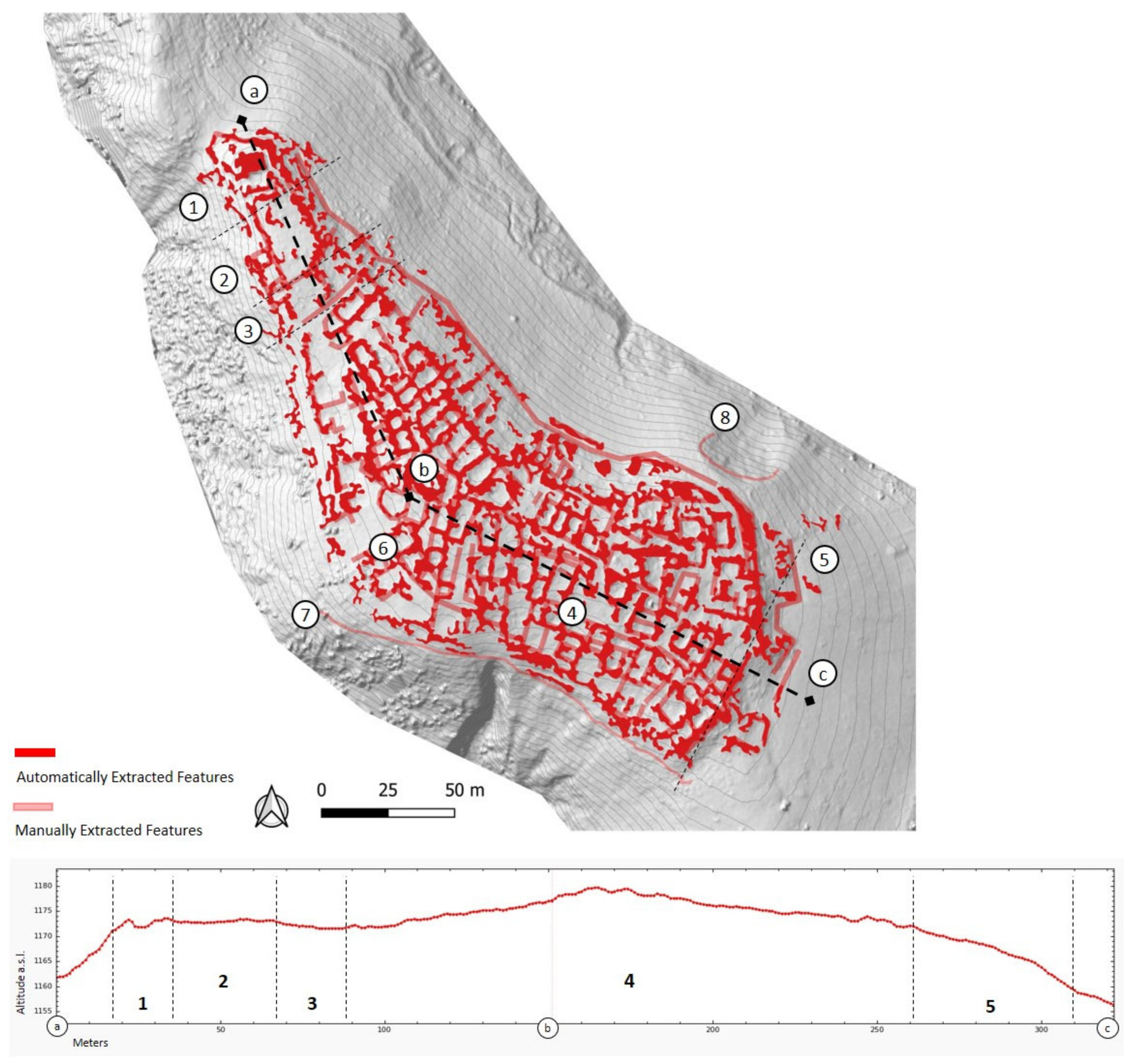
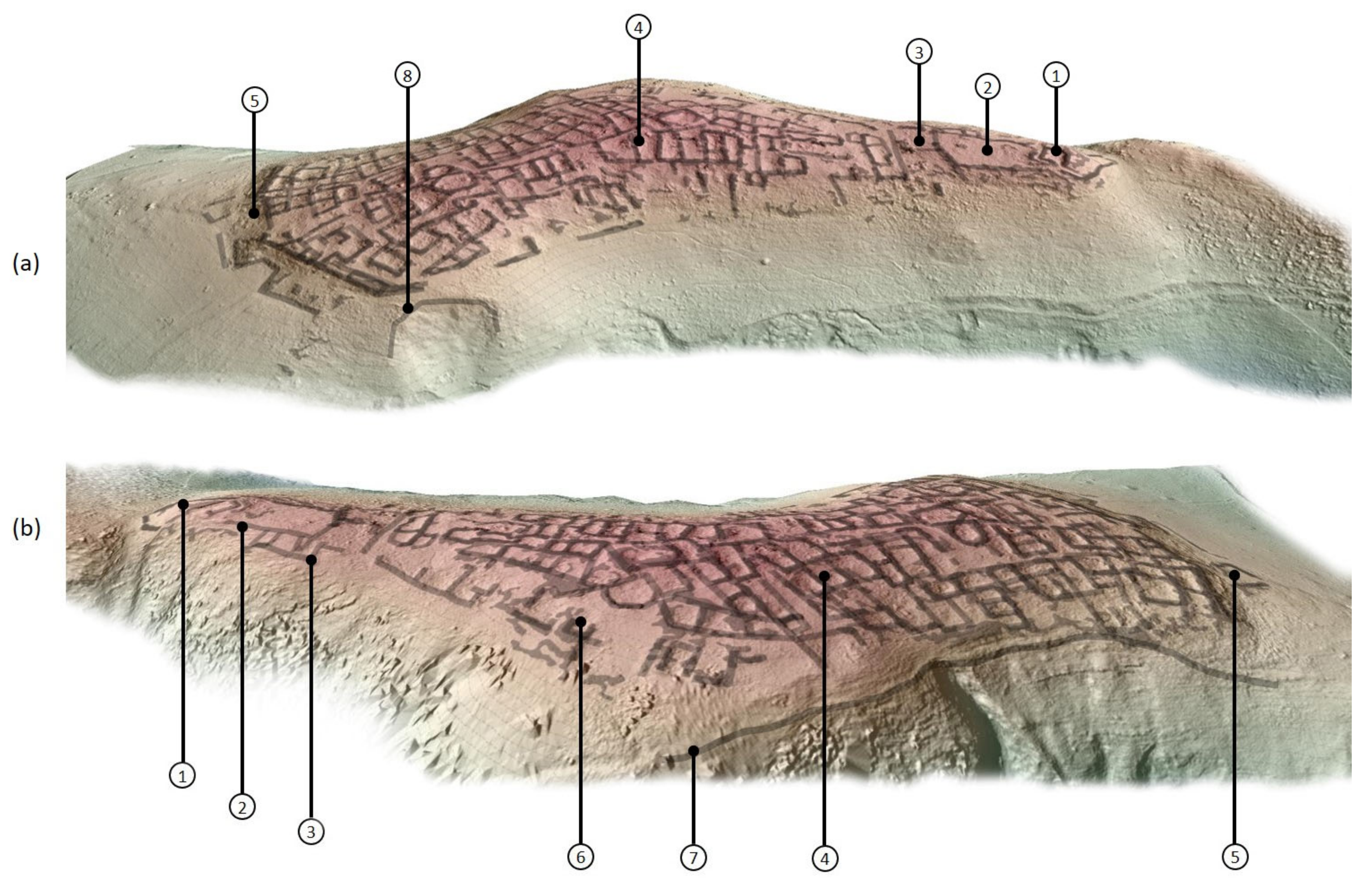
3.3. Archaeological Analysis of the Identified Features
4. Conclusions
- The resolution of the LiDAR data from the drone is abundantly sufficient to recognize microtopographic features of archaeological interest, even in a context such as Perticara, characterized by such high-wooded cover;
- The automatic approach of extracting the same features, compared with the qualitative interpretation (in turn corroborated by ground validation), has proven to be effective and therefore mature to be used in operational scenarios of preventive archeology;
- From an archaeological point of view, the application has allowed the reconstruction of the urban form, and the identification of its constituent elements from a constructive and functional point of view.
Author Contributions
Funding
Data Availability Statement
Acknowledgments
Conflicts of Interest
References
- Chase, A.F.; Chase, D.Z.; Weishampel, J.F.; Drake, J.B.; Shrestha, R.L.; Slatton, K.C.; Awe, J.J.; Carter, W.E. Airborne LiDAR, Archaeology, and the Ancient Maya Landscape at Caracol, Belize. J. Archaeol. Sci. 2011, 38, 387–398. [Google Scholar] [CrossRef]
- Doneus, M.; Briese, C.; Fera, M.; Janner, M. Archaeological Prospection of Forested Areas Using Full-Waveform Airborne Laser Scanning. J. Archaeol. Sci. 2008, 35, 882–893. [Google Scholar] [CrossRef]
- Evans, D.; Traviglia, A. Uncovering Angkor: Integrated Remote Sensing Applications in the Archaeology of Early Cambodia. In Satellite Remote Sensing; Remote Sensing and Digital Image Processing; Lasaponara, R., Masini, N., Eds.; Springer: Dordrecht, The Netherlands, 2012; Volume 16, pp. 197–230. ISBN 978-90-481-8800-0. [Google Scholar]
- Masini, N.; Gizzi, F.; Biscione, M.; Fundone, V.; Sedile, M.; Sileo, M.; Pecci, A.; Lacovara, B.; Lasaponara, R. Medieval Archaeology Under the Canopy with LiDAR. The (Re)Discovery of a Medieval Fortified Settlement in Southern Italy. Remote Sens. 2018, 10, 1598. [Google Scholar] [CrossRef] [Green Version]
- Masini, N.; Lasaponara, R. On the Reuse of Multiscale LiDAR Data to Investigate the Resilience in the Late Medieval Time: The Case Study of Basilicata in South of Italy. J. Archaeol. Method Theory 2021, 28, 1172–1199. [Google Scholar] [CrossRef]
- Chase, A.; Chase, D.; Chase, A. Ethics, New Colonialism, and Lidar Data: A Decade of Lidar in Maya Archaeology. J. Comput. Appl. Archaeol. 2020, 3, 51–62. [Google Scholar] [CrossRef]
- Crutchley, S. Light Detection and Ranging (Lidar) in the Witham Valley, Lincolnshire: An Assessment of New Remote Sensing Techniques. Archaeol. Prospect. 2006, 13, 251–257. [Google Scholar] [CrossRef]
- Devereux, B.J.; Amable, G.S.; Crow, P.; Cliff, A.D. The Potential of Airborne Lidar for Detection of Archaeological Features under Woodland Canopies. Antiquity 2005, 79, 648–660. [Google Scholar] [CrossRef]
- Canuto, M.A.; Estrada-Belli, F.; Garrison, T.G.; Houston, S.D.; Acuña, M.J.; Kováč, M.; Marken, D.; Nondédéo, P.; Auld-Thomas, L.; Castanet, C.; et al. Ancient Lowland Maya Complexity as Revealed by Airborne Laser Scanning of Northern Guatemala. Science 2018, 361, eaau0137. [Google Scholar] [CrossRef] [PubMed] [Green Version]
- Rosenswig, R.M.; López-Torrijos, R. Lidar Reveals the Entire Kingdom of Izapa during the First Millennium BC. Antiquity 2018, 92, 1292–1309. [Google Scholar] [CrossRef]
- Johnson, K.M.; Ouimet, W.B. Rediscovering the Lost Archaeological Landscape of Southern New England Using Airborne Light Detection and Ranging (LiDAR). J. Archaeol. Sci. 2014, 43, 9–20. [Google Scholar] [CrossRef]
- Lozić, E.; Štular, B. Documentation of Archaeology-Specific Workflow for Airborne LiDAR Data Processing. Geosciences 2021, 11, 26. [Google Scholar] [CrossRef]
- Štular, B.; Eichert, S.; Lozić, E. Airborne LiDAR Point Cloud Processing for Archaeology. Pipeline and QGIS Toolbox. Remote Sens. 2021, 13, 3225. [Google Scholar] [CrossRef]
- Doneus, M.; Mandlburger, G.; Doneus, N. Archaeological Ground Point Filtering of Airborne Laser Scan Derived Point-Clouds in a Difficult Mediterranean Environment. J. Comput. Appl. Archaeol. 2020, 3, 92–108. [Google Scholar] [CrossRef] [Green Version]
- Fernandez-Diaz, J.C.; Carter, W.E.; Shrestha, R.L.; Glennie, C.L. Now You See It… Now You Don’t: Understanding Airborne Mapping LiDAR Collection and Data Product Generation for Archaeological Research in Mesoamerica. Remote Sens. 2014, 6, 9951–10001. [Google Scholar] [CrossRef] [Green Version]
- Grammer, B.; Draganits, E.; Gretscher, M.; Muss, U. LiDAR-Guided Archaeological Survey of a Mediterranean Landscape: Lessons from the Ancient Greek Polis of Kolophon (Ionia, Western Anatolia). Archaeol. Prospect. 2017, 24, 311–333. [Google Scholar] [CrossRef] [Green Version]
- Crutchley, S. The Light Fantastic—Using Airborne Lidar in Archaeological Survey. In Proceedings of the ISPRS TC VII Symposium—100 Years ISPRS, Vienna, Austria, 5–7 July 2010; Volume 38. [Google Scholar]
- Strayer, J.R. Dictionary of the Middle Ages; C. Scribner’s Sons: New York, NY, USA, 1982; ISBN 978-0-684-19073-0. [Google Scholar]
- Boserup, E. The Conditions of Agricultural Growth; Routledge: London, UK, 2017; ISBN 978-1-351-48454-1. [Google Scholar]
- Beresford, M. (Ed.) Deserted Medieval Villages: Studies; Sutton: Gloucester, UK, 1989; ISBN 978-0-86299-655-0. [Google Scholar]
- Klapisch-Zuber, C.; Day, J. Villages Désertés En Italie. In Villages Désertés et Histoire Économique (XI-XVIII Siècle); S.E.V.P.N.: Paris, France, 1965; pp. 419–460. [Google Scholar]
- Milanese, M. (Ed.) Vita e Morte dei Villaggi Rurali tra Medioevo ed età Moderna: Dallo Scavo Della Villa de GERITI ad Una Pianificazione Della Tutela e Della Conoscenza dei Villaggi Abbandonati Della Sardegna; Quaderni del Centro di documentazione dei villaggi abbandonati della Sardegna; All’insegna del giglio: Borgo San Lorenzo, Italy, 2006; ISBN 978-88-7814-333-3. [Google Scholar]
- Lasaponara, R.; Masini, N. Full-Waveform Airborne Laser Scanning for the Detection of Medieval Archaeological Microtopographic Relief. J. Cult. Herit. 2009, 10, e78–e82. [Google Scholar] [CrossRef]
- Lasaponara, R.; Coluzzi, R.; Gizzi, F.T.; Masini, N. On the LiDAR Contribution for the Archaeological and Geomorphological Study of a Deserted Medieval Village in Southern Italy. J. Geophys. Eng. 2010, 7, 155–163. [Google Scholar] [CrossRef]
- Guth, P.L.; Van Niekerk, A.; Grohmann, C.H.; Muller, J.-P.; Hawker, L.; Florinsky, I.V.; Gesch, D.; Reuter, H.I.; Herrera-Cruz, V.; Riazanoff, S.; et al. Digital Elevation Models: Terminology and Definitions. Remote Sens. 2021, 13, 3581. [Google Scholar] [CrossRef]
- Zakšek, K.; Oštir, K.; Kokalj, Ž. Sky-View Factor as a Relief Visualization Technique. Remote Sens. 2011, 3, 398–415. [Google Scholar] [CrossRef] [Green Version]
- Hesse, R. LiDAR-Derived Local Relief Models—A New Tool for Archaeological Prospection. Archaeol. Prospect. 2010, 17, 67–72. [Google Scholar] [CrossRef]
- Doneus, M. Openness as Visualization Technique for Interpretative Mapping of Airborne Lidar Derived Digital Terrain Models. Remote Sens. 2013, 5, 6427–6442. [Google Scholar] [CrossRef] [Green Version]
- Danese, M.; Gioia, D.; Vitale, V.; Abate, N.; Amodio, A.M.; Lasaponara, R.; Masini, N. Pattern Recognition Approach and LiDAR for the Analysis and Mapping of Archaeological Looting: Application to an Etruscan Site. Remote Sens. 2022, 14, 1587. [Google Scholar] [CrossRef]
- Küçükdemirci, M.; Landeschi, G.; Ohlsson, M.; Dell’Unto, N. Investigating Ancient Agricultural Field Systems in Sweden from Airborne LIDAR Data by Using Convolutional Neural Network. Archaeol. Prospect. 2022. [Google Scholar] [CrossRef]
- Verschoof-van der Vaart, W.B.; Lambers, K. Learning to Look at LiDAR: The Use of R-CNN in the Automated Detection of Archaeological Objects in LiDAR Data from the Netherlands. J. Comput. Appl. Archaeol. 2019, 2, 31–40. [Google Scholar] [CrossRef] [Green Version]
- Guyot, A.; Lennon, M.; Lorho, T.; Hubert-Moy, L. Combined Detection and Segmentation of Archeological Structures from LiDAR Data Using a Deep Learning Approach. J. Comput. Appl. Archaeol. 2021, 4, 1. [Google Scholar] [CrossRef]
- Pedio, T. La Basilicata Dalla Caduta Dell’Impero Romano Agli Angioini, I.; Levante Editori: Bari, Italy, 1987. [Google Scholar]
- Lapadula, E. L’Alta Valle Del Sauro e Il Tempa Rossa Project (Basilicata, Corleto Perticara, PZ): Alcuni Dati per La Ricostruzione Del Paesaggio Tra Tardo Antico e Medio Evo. In Proceedings of the Atti del VII Congresso Nazionale di Archeologia Medievale, Lecce, Italy, 9–12 September 2015; Volume 1, pp. 459–464. [Google Scholar]
- Sogliani, F. Il Mondo Rurale Della Basilicata Nel Medioevo. La Lettura Archeologica Della Compagine Insediativa, Delle Modalità Di Controllo e Sfruttamento Territoriale e Dei Sistemi Socio-Economici Delle Campagne Tra X e XIII Secolo. Archeol. Mediev. 2010, 37, 171–195. [Google Scholar]
- Gizzi, F.T.; Bentivenga, M.; Lasaponara, R.; Danese, M.; Potenza, M.R.; Sileo, M.; Masini, N. Natural Hazards, Human Factors, and “Ghost Towns”: A Multi-Level Approach. Geoheritage 2019, 11, 1533–1565. [Google Scholar] [CrossRef]
- Patacca, E.; Scandone, P. Geology of the Southern Apennines. Boll. Della Soc. Geol. Ital. 2007, 7, 75–119. [Google Scholar]
- Cruden, D.; Cruden, D.M.; Varnes, D.J. Landslide Types and Processes. In Transportation Research Board, U.S. National Academy of Sciences, Special Report; Transportation Research Board, U.S. National Academy of Sciences: Washington, DC, USA, 1996; Volume 247, pp. 36–75. [Google Scholar]
- Bentivenga, M.; Palladino, G.; Caputi, A. Development of Pietra Maura landslide and interactions with the Marsico Nuovo dam (Basilicata, Italy). Geogr. Fis. Din. Quat. 2012, 35, 13–22. [Google Scholar] [CrossRef]
- Bentivenga, M.; Prosser, G.; Gugliemi, P.; Palladino, G.; Piccarreta, M.; Straziuso, K.; Cavalcante, F. Landslide Inventory Maps and Relationship with Predisposing Factors: A Case Study from the Southern Apennines, Italy. J. Maps 2022. [Google Scholar] [CrossRef]
- Tarquini, S.; Isola, I.; Favalli, M.; Mazzarini, F.; Bisson, M.; Pareschi, M.T.; Boschi, E. TINITALY/01: A New Triangular Irregular Network of Italy. Ann. Geophys. 2009, 50, 407–425. [Google Scholar] [CrossRef]
- Tarquini, S.; Vinci, S.; Favalli, M.; Doumaz, F.; Fornaciai, A.; Nannipieri, L. Release of a 10-m-Resolution DEM for the Italian Territory: Comparison with Global-Coverage DEMs and Anaglyph-Mode Exploration via the Web. Comput. Geosci. 2012, 38, 168–170. [Google Scholar] [CrossRef]
- Tarquini, S.; Isola, I.; Favalli, M.; Battistini, A. TINITALY, a Digital Elevation Model of Italy with a 10 Meters Cell Size 2007, about 3000 M Grid Cells, about 17 Gb of Disk Memory; Istituto Nazionale di Geofisica e Vulcanologia: Roma, Italy, 2007. [Google Scholar]
- Tarquini, S.; Nannipieri, L. The 10m-Resolution TINITALY DEM as a Trans-Disciplinary Basis for the Analysis of the Italian Territory: Current Trends and New Perspectives. Geomorphology 2017, 281, 108–115. [Google Scholar] [CrossRef]
- Štular, B.; Lozić, E. Comparison of Filters for Archaeology-Specific Ground Extraction from Airborne LiDAR Point Clouds. Remote Sens. 2020, 12, 3025. [Google Scholar] [CrossRef]
- Zhang, K.; Chen, S.-C.; Whitman, D.; Shyu, M.-L.; Yan, J.; Zhang, C. A Progressive Morphological Filter for Removing Nonground Measurements from Airborne LIDAR Data. IEEE Trans. Geosci. Remote Sens. 2003, 41, 872–882. [Google Scholar] [CrossRef] [Green Version]
- Shan, J.; Toth, C. Topographic Laser Ranging and Scanning: Principles and Processing; CRC Press: Boca Raton, FL, USA, 2018. [Google Scholar]
- Sithole, G.; Vosselman, G. Experimental Comparison of Filter Algorithms for Bare-Earth Extraction from Airborne Laser Scanning Point Clouds. ISPRS J. Photogramm. Remote Sens. 2004, 59, 85–101. [Google Scholar] [CrossRef]
- Buján, S.; Cordero, M.; Miranda, D. Hybrid Overlap Filter for LiDAR Point Clouds Using Free Software. Remote Sens. 2020, 12, 1051. [Google Scholar] [CrossRef] [Green Version]
- Axelsson, P. DEM Generation from Laser Scanner Data Using Adaptive TIN Models. Int. Arch. Photogramm. Remote Sens. 2000, 33, 110–117. [Google Scholar]
- Briese, C.; Pfeifer, N. Airborne Laser Scanning and Derivation of Digital Terrain Models. In Proceedings of the 5th Conference on Optical 3D Measurement Techniques, Vienna, Austria, 1–4 October 2001; pp. 80–87. [Google Scholar]
- Suleymanoglu, B.; Soycan, M. Comparison of Filtering Algorithms Used for DTM Production from Airborne Lidar Data: A Case Study in Bergama, Turkey. Geod. Vestn. 2019, 63, 395–414. [Google Scholar] [CrossRef]
- Rasterize—CloudCompareWiki. Available online: https://www.cloudcompare.org/doc/wiki/index.php/Rasterize (accessed on 30 October 2022).
- Masini, N.; Coluzzi, R.; Lasaponar, R. On the Airborne Lidar Contribution in Archaeology: From Site Identification to Landscape Investigation. In Laser Scanning, Theory and Applications; Wang, C.-C., Ed.; InTech: London, UK, 2011; ISBN 978-953-307-205-0. [Google Scholar]
- Štular, B.; Lozić, E.; Eichert, S. Airborne LiDAR-Derived Digital Elevation Model for Archaeology. Remote Sens. 2021, 13, 1855. [Google Scholar] [CrossRef]
- Kokalj, Ž.; Zakšek, K.; Oštir, K.; Pehani, P.; Čotar, K.; Somrak, M. Relief Visualization Toolbox, Ver. 2.2.1 Manual. 11. Remote Sens 2016, 3, 398–415. [Google Scholar]
- Kokalj, Ž.; Hesse, R. Airborne Laser Scanning Raster Data Visualization; Prostor, Kraj, Čas; ZRC SAZU, Založba ZRC, Banka Slovenije: Ljubljana, Slovenia, 2017; Volume 14, ISBN 978-961-254-984-8. [Google Scholar]
- Lee, J.-S. Digital Image Enhancement and Noise Filtering by Use of Local Statistics. IEEE Trans. Pattern Anal. Mach. Intell. 1980, PAMI-2, 165–168. [Google Scholar] [CrossRef] [PubMed] [Green Version]
- Lopes, A.; Touzi, R.; Nezry, E. Adaptive Speckle Filters and Scene Heterogeneity. IEEE Trans. Geosci. Remote Sens. 1990, 28, 992–1000. [Google Scholar] [CrossRef]
- Davis, D.S.; Sanger, M.C.; Lipo, C.P. Automated Mound Detection Using Lidar and Object-Based Image Analysis in Beaufort County, South Carolina. Southeast. Archaeol. 2019, 38, 23–37. [Google Scholar] [CrossRef]
- Conrad, O.; Bechtel, B.; Bock, M.; Dietrich, H.; Fischer, E.; Gerlitz, L.; Wehberg, J.; Wichmann, V.; Böhner, J. System for Automated Geoscientific Analyses (SAGA) v. 2.1.4. Geosci. Model Dev. 2015, 8, 1991–2007. [Google Scholar] [CrossRef] [Green Version]
- Ahsan, M.M.; Mahmud, M.A.P.; Saha, P.K.; Gupta, K.D.; Siddique, Z. Effect of Data Scaling Methods on Machine Learning Algorithms and Model Performance. Technologies 2021, 9, 52. [Google Scholar] [CrossRef]
- Jo, J.-M. Effectiveness of Normalization Pre-Processing of Big Data to the Machine Learning Performance. J. Korea Inst. Electron. Commun. Sci. 2019, 14, 547–552. [Google Scholar] [CrossRef]
- Ali, P.J.M.; Faraj, R.H. Data Normalization and Standardization: A Technical Report. Mach. Learn. Tech. Rep. 2014, 1, 1–6. [Google Scholar] [CrossRef]
- Sola, J.; Sevilla, J. Importance of Input Data Normalization for the Application of Neural Networks to Complex Industrial Problems. IEEE Trans. Nucl. Sci. 1997, 44, 1464–1468. [Google Scholar] [CrossRef]
- Lasaponara, R.; Masini, N. (Eds.) Satellite Remote Sensing: A New Tool for Archaeology; Remote Sensing and Digital Image Processing; Springer: Dordrecht, The Netherlands; New York, NY, USA, 2012; ISBN 978-90-481-8800-0. [Google Scholar]
- Klassen, S.; Weed, J.; Evans, D. Semi-Supervised Machine Learning Approaches for Predicting the Chronology of Archaeological Sites: A Case Study of Temples from Medieval Angkor, Cambodia. PLoS ONE 2018, 13, e0205649. [Google Scholar] [CrossRef] [Green Version]
- Keeney, J.; Hickey, R. Using Satellite Image Analysis for Locating Prehistoric Archaeological Sites in Alaska’s Central Brooks Range. J. Archaeol. Sci. Rep. 2015, 3, 80–89. [Google Scholar] [CrossRef] [Green Version]
- Jensen, J.R. Introductory Digital Image Processing: A Remote Sensing Perspective; Pearson Series in Geographic Information Science; Pearson Education, Inc: Glenview, IL, USA, 2016; ISBN 978-0-13-405816-0. [Google Scholar]
- Lillesand, T.M.; Kiefer, R.W.; Chipman, J.W. Remote Sensing and Image Interpretation, 7th ed.; John Wiley & Sons, Inc: Hoboken, NJ, USA, 2015; ISBN 978-1-118-34328-9. [Google Scholar]
- Hadjimitsis, D.G.; Themistocleous, K.; Cuca, B.; Agapiou, A.; Lysandrou, V.; Lasaponara, R.; Masini, N.; Schreier, G. (Eds.) Remote Sensing for Archaeology and Cultural Landscapes: Best Practices and Perspectives Across Europe and the Middle East; Springer Remote Sensing/Photogrammetry; Springer International Publishing: Cham, Switzerland, 2020; ISBN 978-3-030-10978-3. [Google Scholar]
- Parcak, S.H. Satellite Remote Sensing for Archaeology; Routledge: London, UK; New York, NY, USA, 2009; ISBN 978-0-415-44877-2. [Google Scholar]
- Lasaponara, R.; Abate, N.; Masini, N. On the Use of Google Earth Engine and Sentinel Data to Detect “Lost” Sections of Ancient Roads. The Case of Via Appia. IEEE Geosci. Remote Sens. Lett. 2021, 19, 3001605. [Google Scholar] [CrossRef]
- Lasaponara, R.; Masini, N. Space-Based Identification of Archaeological Illegal Excavations and a New Automatic Method for Looting Feature Extraction in Desert Areas. Surv. Geophys. 2018, 39, 1323–1346. [Google Scholar] [CrossRef]
- Anselin, L. Local Indicators of Spatial Association—LISA. Geogr. Anal. 1995, 27, 93–115. [Google Scholar] [CrossRef]
- Ord, J.K.; Getis, A. Local Spatial Autocorrelation Statistics: Distributional Issues and an Application. Geogr. Anal. 1995, 27, 286–306. [Google Scholar] [CrossRef]
- Srinivasan, S. Local and Global Spatial Statistics. In Encyclopedia of GIS; Shekhar, S., Xiong, H., Eds.; Springer: Boston, MA, USA, 2008; p. 615. ISBN 978-0-387-30858-6. [Google Scholar]
- Davis, D.S. Object-based Image Analysis: A Review of Developments and Future Directions of Automated Feature Detection in Landscape Archaeology. Archaeol. Prospect. 2019, 26, 155–163. [Google Scholar] [CrossRef]
- Richards-Rissetto, H.; Newton, D.; Al Zadjali, A. A 3D point cloud deep learning approach using lidar to identify ancient maya archaeological sites. ISPRS Ann. Photogramm. Remote Sens. Spat. Inf. Sci. 2021, VIII-M-1–2021, 133–139. [Google Scholar] [CrossRef]
- Guyot, A.; Lennon, M.; Hubert-Moy, L. Objective Comparison of Relief Visualization Techniques with Deep CNN for Archaeology. J. Archaeol. Sci. Rep. 2021, 38, 103027. [Google Scholar] [CrossRef]
- Trotter, E.; Fernandes, A.; Fibæk, C.; Keßler, C. Machine Learning for Automatic Detection of Historic Stone Walls Using LiDAR Data. Int. J. Remote Sens. 2022, 43, 2185–2211. [Google Scholar] [CrossRef]
- Vitale, V. Il Paesaggio Medievale Nella Basilicata Meridionale: Le Forme Del Potere Laico Ed Ecclesiastico Nella Media Valle Del Sinni Tra X e XV Secolo d.C; BAR International Series; BAR Publishing: Oxford, UK, 2021; ISBN 978-1-4073-5762-1. [Google Scholar]
- Frisetti, A.; Cuomo, M.; Abate, N. Archeologia Ed Analisi Dei Contesti Fortificati in Campania: Il Caso Del Castello Di Roccaromana; Edizioni EBS: Arcore, Italy, 2019; pp. 322–327. [Google Scholar]


| Visualization Method | Parameters |
|---|---|
| Analytical Hillshading | Sun azimuth (deg): 315; Sun elevation angle (deg): 35 |
| Hillshading from Multiple Directions | Number of directions: 16; Sun elevation angle (deg): 35 |
| PCA of Hillshading | Number of components to save: 3 |
| Slope Gradient | No parameters required |
| Simple Local Relief Model | Radius for trend assessment (pixel): 20 |
| Sky-View Factor | Number of search directions: 16; search radius (pixel): 20 |
| Openness Positive | Number of search directions: 16; search radius (pixel): 20 |
| Openness Negative | Number of search directions: 16; search radius (pixel): 20 |
| Archaeological (VAT) | Used preset: general |
| xi | L (m) | OP (m) | SLRM (m) | PCA (m) | SVF (m) | Slope (m) | VAT (m) | µOP | µSLRM | µPCA | µSVF | µSlope | µVAT | ||
|---|---|---|---|---|---|---|---|---|---|---|---|---|---|---|---|
| Wall and perimeter features | W1 | 28.3 | 28.4 | 28 | 26.7 | 27.8 | 28.8 | 28.8 | 0.0018 | −0.0053 | −0.0291 | −0.0089 | 0.0088 | 0.0088 | |
| W2 | 21.1 | 21.1 | 22 | 21.6 | 21.9 | 21.3 | 21 | 0.0000 | 0.0209 | 0.0117 | 0.0186 | 0.0047 | −0.0024 | ||
| W3 | 52.6 | 52.8 | 49.2 | 50.1 | 52.4 | 48.1 | 52 | 0.0019 | −0.0334 | −0.0243 | −0.0019 | −0.0447 | −0.0057 | ||
| W4 | 19.2 | 10 | 17.4 | 16.5 | 17.6 | 16.8 | 15.8 | −0.3151 | −0.0492 | −0.0756 | −0.0435 | −0.0667 | −0.0971 | ||
| W5 | 32 | 33 | 36 | 30.6 | 33.1 | 23.4 | 32.1 | 0.0154 | 0.0588 | −0.0224 | 0.0169 | −0.1552 | 0.0016 | ||
| W6 | 48.6 | 39.7 | 31.1 | 44.4 | 48 | 49 | 46.4 | −0.1008 | −0.2196 | −0.0452 | −0.0062 | 0.0041 | −0.0232 | ||
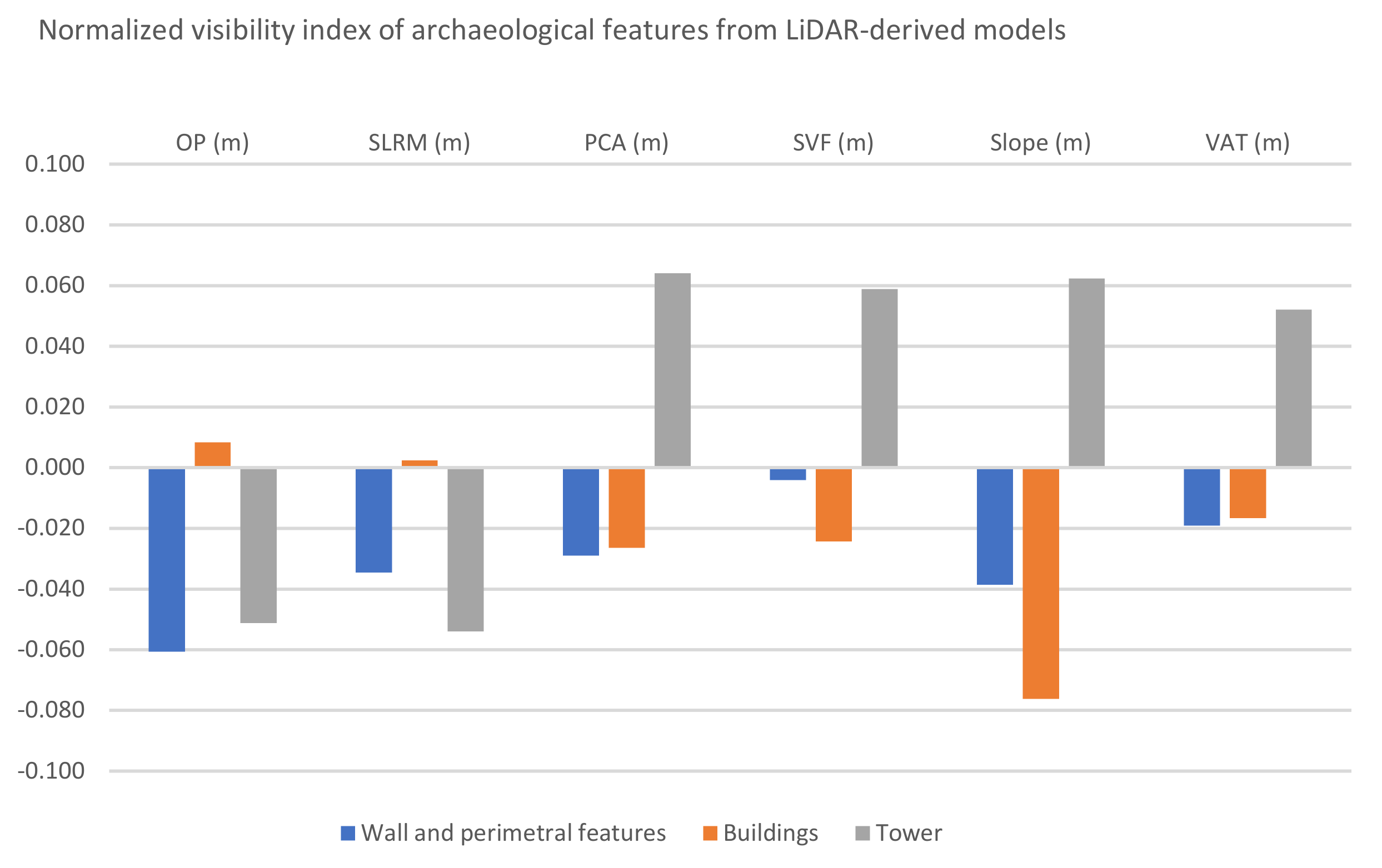
| ∑Lw | µLDM | −0.032 | −0.034 | −0.028 | −0.002 | −0.031 | −0.013 | ||||||||
| −3.20% | −3.4% | −2.8% | −0.20% | −3.10% | −1.3% | ||||||||||
| Buildings | B1 | 83 | 78.3 | 83.8 | 49 | 75 | 83.2 | 82 | −0.0291 | 0.0048 | −0.2576 | −0.0506 | 0.0012 | −0.0061 | |
| B2 | 14.7 | 13.5 | 13.8 | 10.7 | 11.8 | 12.4 | 13.9 | −0.0426 | −0.0316 | −0.1575 | −0.1094 | −0.0849 | −0.0280 | ||
| B3 | 16 | 14.7 | 14.6 | 11.6 | 12.3 | 11 | 12.4 | −0.0423 | −0.0458 | −0.1594 | −0.1307 | −0.1852 | −0.1268 | ||
| B4 | 17.9 | 19.2 | 20 | 17.7 | 16.3 | 15.3 | 15.8 | 0.0350 | 0.0554 | −0.0056 | −0.0468 | −0.0783 | −0.0623 | ||
| B5 | 22 | 21.3 | 21.3 | 19.9 | 20 | 19.5 | 20.5 | −0.0162 | −0.0162 | −0.0501 | −0.0476 | −0.0602 | −0.0353 | ||
| B6 | 14 | 13.5 | 13.1 | 13.4 | 13.6 | 12.9 | 12.9 | −0.0182 | −0.0332 | −0.0219 | −0.0145 | −0.0409 | −0.0409 | ||
| B7 | 7.9 | 7.5 | 7.5 | 7.6 | 7.5 | 7.1 | 7.6 | −0.0260 | −0.0260 | −0.0194 | −0.0260 | −0.0533 | −0.0194 | ||
| B8 | 19 | 21 | 21.8 | 18.4 | 18.1 | 17.1 | 18.8 | 0.0500 | 0.0686 | −0.0160 | −0.0243 | −0.0526 | −0.0053 | ||
| B9 | 48 | 49.5 | 49.1 | 46.9 | 46.1 | 46.1 | 48.5 | 0.0154 | 0.0113 | −0.0116 | −0.0202 | −0.0202 | 0.0052 | ||
| B10 | 9.6 | 6.9 | 9.1 | 8.4 | 8.6 | 7.9 | 8.8 | −0.1636 | −0.0267 | −0.0667 | −0.0549 | −0.0971 | −0.0435 | ||
| B11 | 15.6 | 22.9 | 15.1 | 22 | 23.6 | 20.9 | 21.8 | 0.1896 | −0.0163 | 0.1702 | 0.2041 | 0.1452 | 0.1658 | ||
| B12 | 32.9 | 31.1 | 31.1 | 31.8 | 26.6 | 26.1 | 30.3 | −0.0281 | −0.0281 | −0.0170 | −0.1059 | −0.1153 | −0.0411 | ||
| B13 | 64.8 | 66 | 58.7 | 64.1 | 59.3 | 0 | 61.6 | 0.0092 | −0.0494 | −0.0054 | −0.0443 | −1.0000 | −0.0253 | ||
| B14 | 31.2 | 30.9 | 31.7 | 30.8 | 29.3 | 30.6 | 26.5 | −0.0048 | 0.0079 | −0.0065 | −0.0314 | −0.0097 | −0.0815 | ||
| B15 | 14.1 | 14.7 | 14.9 | 13.7 | 13.4 | 13.4 | 13.4 | 0.0208 | 0.0276 | −0.0144 | −0.0255 | −0.0255 | −0.0255 | ||
| B16 | 26.1 | 25.9 | 25.3 | 24.4 | 24.6 | 24.1 | 25.2 | −0.0038 | −0.0156 | −0.0337 | −0.0296 | −0.0398 | −0.0175 | ||
| B17 | 11.7 | 15.9 | 15.8 | 14.4 | 15.1 | 11.5 | 14.7 | 0.1522 | 0.1491 | 0.1034 | 0.1269 | −0.0086 | 0.1136 | ||
| B18 | 12 | 13 | 12.4 | 11.9 | 12 | 12 | 12.6 | 0.0400 | 0.0164 | −0.0042 | 0.0000 | 0.0000 | 0.0244 | ||
| B19 | 10.6 | 12 | 10.8 | 11 | 10.4 | 9.4 | 10.4 | 0.0619 | 0.0093 | 0.0185 | −0.0095 | −0.0600 | −0.0095 | ||
| B20 | 17.9 | 16.7 | 17.4 | 17 | 15.3 | 14.6 | 15.1 | −0.0347 | −0.0142 | −0.0258 | −0.0783 | −0.1015 | −0.0848 | ||
| ∑Lw | µLDM | 0.0088 | −0.0002 | −0.0332 | −0.0259 | −0.0257 | −0.0135 | ||||||||
| 0.88% | −0.02% | −3.32% | −2.59% | −2.57% | −1.35% | ||||||||||
| Tower | T1 | 32.2 | 28.7 | 28.5 | 36.1 | 35.8 | 36 | 35.4 | −0.0575 | −0.0610 | 0.0571 | 0.0529 | 0.0557 | 0.0473 | |
| ∑Lw | µLDM | −0.0512 | −0.0540 | 0.0640 | 0.0589 | 0.0623 | 0.0520 | ||||||||
| −5.12% | −5.4% | 6.4% | 5.89% | 6.23% | 5.2% |
Publisher’s Note: MDPI stays neutral with regard to jurisdictional claims in published maps and institutional affiliations. |
© 2022 by the authors. Licensee MDPI, Basel, Switzerland. This article is an open access article distributed under the terms and conditions of the Creative Commons Attribution (CC BY) license (https://creativecommons.org/licenses/by/4.0/).
Share and Cite
Masini, N.; Abate, N.; Gizzi, F.T.; Vitale, V.; Minervino Amodio, A.; Sileo, M.; Biscione, M.; Lasaponara, R.; Bentivenga, M.; Cavalcante, F. UAV LiDAR Based Approach for the Detection and Interpretation of Archaeological Micro Topography under Canopy—The Rediscovery of Perticara (Basilicata, Italy). Remote Sens. 2022, 14, 6074. https://doi.org/10.3390/rs14236074
Masini N, Abate N, Gizzi FT, Vitale V, Minervino Amodio A, Sileo M, Biscione M, Lasaponara R, Bentivenga M, Cavalcante F. UAV LiDAR Based Approach for the Detection and Interpretation of Archaeological Micro Topography under Canopy—The Rediscovery of Perticara (Basilicata, Italy). Remote Sensing. 2022; 14(23):6074. https://doi.org/10.3390/rs14236074
Chicago/Turabian StyleMasini, Nicola, Nicodemo Abate, Fabrizio Terenzio Gizzi, Valentino Vitale, Antonio Minervino Amodio, Maria Sileo, Marilisa Biscione, Rosa Lasaponara, Mario Bentivenga, and Francesco Cavalcante. 2022. "UAV LiDAR Based Approach for the Detection and Interpretation of Archaeological Micro Topography under Canopy—The Rediscovery of Perticara (Basilicata, Italy)" Remote Sensing 14, no. 23: 6074. https://doi.org/10.3390/rs14236074