
Improved Central Attention Network-Based Tensor RX for Hyperspectral Anomaly Detection
1
College of Mechanical and Electrical Engineering, Daqing Normal University, Daqing 163712, China
2
School of Computer Science and Technology, Heilongjiang University, Harbin 150080, China
*
Author to whom correspondence should be addressed.
Remote Sens. 2022, 14(22), 5865; https://doi.org/10.3390/rs14225865
Submission received: 24 October 2022
/
Revised: 11 November 2022
/
Accepted: 17 November 2022
/
Published: 19 November 2022
(This article belongs to the Special Issue Artificial Intelligence Algorithm for Remote Sensing Imagery Processing Ⅱ)
Abstract
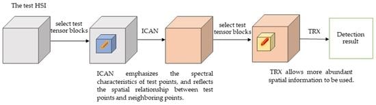
:Recently, using spatial–spectral information for hyperspectral anomaly detection (AD) has received extensive attention. However, the test point and its neighborhood points are usually treated equally without highlighting the test point, which is unreasonable. In this paper, improved central attention network-based tensor RX (ICAN-TRX) is designed to extract hyperspectral anomaly targets. The ICAN-TRX algorithm consists of two parts, ICAN and TRX. In ICAN, a test tensor block as a value tensor is first reconstructed by DBN to make the anomaly points more prominent. Then, in the reconstructed tensor block, the central tensor is used as a convolution kernel to perform convolution operation with its tensor block. The result tensor as a key tensor is transformed into a weight matrix. Finally, after the correlation operation between the value tensor and the weight matrix, the new test point is obtained. In ICAN, the spectral information of a test point is emphasized, and the spatial relationships between the test point and its neighborhood points reflect their similarities. TRX is used in the new HSI after ICAN, which allows more abundant spatial information to be used for AD. Five real hyperspectral datasets are selected to estimate the performance of the proposed ICAN-TRX algorithm. The detection results demonstrate that ICAN-TRX achieves superior performance compared with seven other AD algorithms.
1. Introduction
Hyperspectral images (HSIs) occupy hundreds of narrow bands in the visible and short-wave infrared region, so they are rich in spectral information [1,2,3,4]. Using this characteristic, HSIs have a strong ability to distinguish ground objects. Classification and target detection are two main applications of HSIs [5]. Target detection belongs to a special case of classification, which is a binary classification. According to whether the target information is known or unknown, there are two types of target detection, and the anomaly target is detected without any prior information [6]. In practical situations, it is challenging to obtain the spectrum of the targets beforehand. Therefore, anomaly detection (AD) has a broader application, such as mineral detection, environmental monitoring, food quality inspection, and search and rescue [7].
Hyperspectral AD mainly depends on the spectral characteristics of HSIs. In recent decades, many algorithms for AD have appeared. The Reed–Xiaoli (RX) algorithm [8] is basic and classic, and the result is derived from the Mahalanobis distance from the test point to the background. It relies on the assumption that the background obeys a multivariate Gaussian distribution. The background of HSIs is usually very complex. Local RX [9] is the local case of RX algorithm, and a sliding-dual window is used for detection. However, for real HSIs, the assumption of Gaussian distribution is usually inaccurate. Some improved algorithms provide new ideas for the estimation of background models, such as a weighted-RXD and a linear filter-based RXD [10]. In addition, many algorithms based on sparse theory do not require model estimation for the HSI data, and they have satisfactory detection results [11,12,13,14,15].
HSIs have both rich spectral information and redundant information. Dimension reduction (DR) is the primary preprocessing method for HSIs. Principal component analysis (PCA) is a famous dimension reduction (DR) algorithm and has been extensively applied [15,16]. It is a linear algorithm. However, HSIs inherent nonlinear features, and PCA may not be able to extract the effective features accurately. To overcome this difficulty, manifold learning is used for hyperspectral AD, and better results are achieved [17,18,19]. Recently, the application of deep learning (DL) theory has received extensive attention [20,21,22]. Hyperspectral AD algorithms using DL for feature extraction have also achieved satisfactory detection performance. Convolutional neural networks (CNN) [23], as typical thoroughly supervised models, improve the results when applied to classification and target detection. In a transferred CNN [24] for AD, reference-labeled samples are used as training datasets because of the lack of training samples. In transferred CNN based on tensor (TCNNT) [25], the test tensor block is treated as a convolutional kernel, so are the local neighboring tensor blocks. TCNNT has been improved into a supervised model. Stacked autoencoders (SAE) [26,27] and deep belief networks (DBNs) [28,29] are unsupervised, and they are more advantageous to hyperspectral AD. In the stacked autoencoders-based adaptive subspace model (SAEASM) [30], the deep features of differences are acquired using SAE architectures. In the fractional Fourier transform and deep belief networks (FDBN)-based AD algorithm [31], DBNs are used for DR and signal reconstruction.
Spectral characteristics play a major role in the above AD algorithms. However, with the progressing of remote sensing technology, HSIs also have better spatial characteristics, and the advantage of spectral characteristics combined with spatial characteristics is emerging [32]. Recently, some AD algorithms using the joint spectral–spatial characteristics have achieved better detection results than only considering the spectral characteristics, such as the spectral–spatial method based on low-rank and sparse matrix decomposition (LS-SS) [33], sparsity divergence index based on locally linear embedding (SDI-LLE) [19], and local summation anomaly detection (LSAD) [34]. In addition, tensor theory has also attracted attention in HSIs processing. To use tensor theory, HSIs are treated as a third-order data cube, which facilitates the simultaneous use of the spatial–spectral characteristics [35]. The coskewness detector (COSD) [36], the low-rank tensor decomposition-based anomaly detection (LTDD) [37], and the tensor decomposition-based algorithm (TenB) [38] mainly rely on tensor decomposition to eliminate redundancy and perform well. The test point and its neighboring pixels are regarded as a test tensor block. Some the methods based on subspace projection [39,40] have been applied to HSI processing and have achieved good results. For hyperspectral AD, the tensor-based adaptive subspace detection (TBASD) algorithm [41] can fully mine the spatial–spectral characteristics while ensuring the relative integrity of the spatial–spectral structure. The tensor RX (TRX) algorithm based on FrFT (FrFT-TRX) [42] uses TRX in the fractional Fourier domain (FrFD). TRX uses the test point tensor, instead of the test point vector, and can better mine spatial characteristics for hyperspectral AD. In the above algorithms involving tensor theory, all the neighboring pixels of a test point in a tensor block are treated equally without highlighting the test point, which is unreasonable. Though the neighboring pixels provide spatial information, the test point should be more important, and its spectral information should be the most important criterion.
Recently, HSIs processing has increasingly adopted self-attention mechanisms, such as bidirectional encoder representations from transformers (BERTHSI) [43] and the multilevel feature network with spectral–spatial attention model (MFNSAM) [44]. To emphasize the importance of a query pixel and ensure the correctness of spatial information extraction from the neighboring pixels of the query pixel at the same time, the central attention network (CAN) has been put forward for hyperspectral imagery classification and obtained superior classification performance [45].
In this paper, improved central attention network-based tensor RX (ICAN-TRX) is presented for hyperspectral AD. The ICAN-TRX algorithm consists of ICAN and TRX. In ICAN, the test tensor block as the value tensor is first reconstructed by DBN to make the anomaly points more prominent. Then, in the reconstructed tensor block, the central tensor is used as a convolution kernel to perform convolution operation with its tensor block, and the result tensor as the key tensor is transformed into the weight matrix. Finally, after the correlation operation between the value tensor and the weight matrix, the new test point is obtained. TRX is used in the new HSI after ICAN.
The highlights of this paper can be summarized in the following three aspects:
- Hyperspectral AD mainly depends on the spectral feature of a test point in HSI. Neighborhood points similar to the test point also contain discriminative information. In ICAN, the spectral information of a test point is emphasized, and spatial information reflects the similarity between the test point and its neighborhood points. The extraction of spectral–spatial features is more reasonable;
- In ICAN, the test point in the center of a test tensor block is used as a convolution kernel to perform convolution operation with the test tensor block, which reflects the similarity between the test point and its neighborhood points. The determination of this convolution kernel avoids the selection of training samples in CNN;
- Because the input of ICAN is the test tensor block, TRX is used after ICAN, which allows more abundant spatial information to be used for AD.
2. The Proposed Methods
2.1. DBN
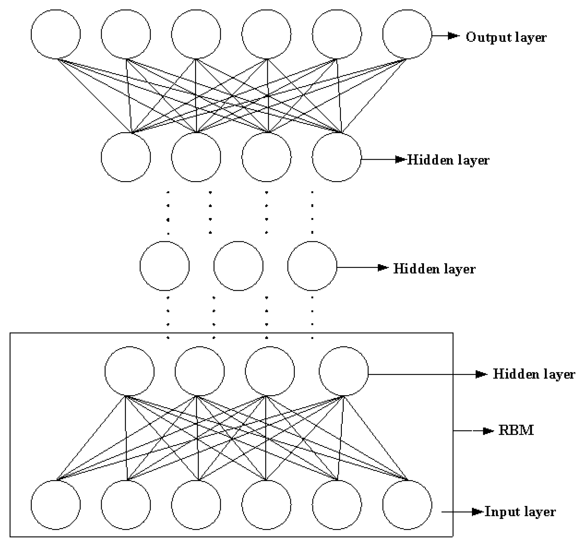
Deep belief networks (DBNs) consist of a multi-layer restricted Boltzmann machines (RBMs) and a layer of back propagation (BP) neural network. Its essence is a specially constructed neural network. In DBNs, the output of the lower level RBM is used as the input of the upper-level RBM, and the output information of the last level RBM network is used as the input data of the BP neural network, as shown in Figure 1.
The training process of DBNs is roughly divided into two steps. The first step is to read the data file, train each layer of the RBM, take the output of the first hidden layer as the input of the visible layer, and then use the output of the visible layer as the input of the next hidden layer for training layer by layer. The separate training of each layer can enable feature vectors to retain more feature information in different feature spaces. The second step is to set the BP neural network at the last layer, receive the output of the RBM as the input of the BP network, and adjust the entire DBNs by updating the neural network parameters from top to bottom to optimize the accuracy of the entire DBNs. Training times, number of samples, and number of layers are three important parameters in DBNs.
Hyperspectral AD is unsupervised target detection. DBNs are an auto-encoder and unsupervised DL model and are more suitable for AD. In this paper, we use the DBNs for the reconstruction of HSIs. Anomaly targets are usually sparse small targets, which have a small probability compared with the background, and their contributions to the DBNs reconstruction model are far less than the background points. Through the DBNs reconstruction, the anomaly points in HSIs are more prominent, which is more conducive to AD.
2.2. Improved Central Attention Module
In the central attention module [45], the test tensor centered on the test point is mapped along the spectral dimension into key and value tensors, respectively. The number of pixels of the two new tensors is equal to that of the test tensor. Every pixel of the key tensor is the key to the corresponding pixel of the test tensor, so is the value tensor. In the improved central attention module, the test tensor is used as the value tensor. For the key tensor, the test tensor is first reconstructed by DBN, and the central tensor in the reconstructed tensor is then used as a convolution kernel to perform convolution operation with the reconstructed tensor. This convolution takes place one time, and the key tensor is obtained. The corresponding weight matrix is transformed from the key tensor. The new tensor is the pointwise multiplication of the value tensor with the weight matrix. The output is a series of transforms of the central tensor in the new tensor. Next, a more detailed description is shown.
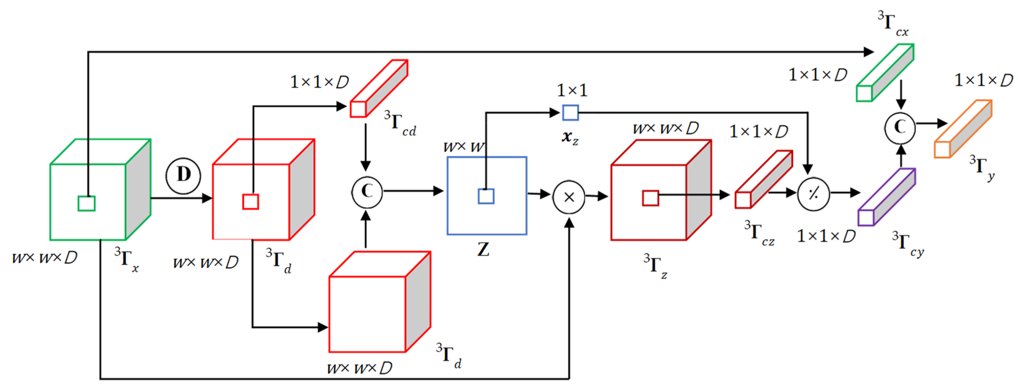
As shown in Figure 2, let ( is the window size of the test tensor, and D is the number of spectral bands) centered at the test point be the test tensor. For DBN reconstruction, the test tensor is first transformed into a pixelwise two-dimensional matrix () that is then reconstructed by DBN. The reconstruction matrix () is transformed into a tensor . The central tensor in is then used as a convolution kernel. It performs convolution operation with , and the convolution takes place one time.
where () is the activation function, is the bias parameter, and is the tensor convolution. The result tensor as the key tensor is transformed into the weight matrix Z.
Next, the test tensor is regarded as the value tensor. The tensor is the pointwise multiplication of and Z that is repeated along spectral dimension D times to adapt to the size of . The tensor is the pointwise division of the central tensor in and the central point in Z. Finally, is used as a convolution kernel and it performs convolution operation with The convolution takes place twice.
where () is the activation function, is the bias parameter, and is the tensor convolution. The tensor is the final output of the ICAN.
In the improved central attention module, the central tensor in the reconstructed tensor using DBNs corresponds to the test point and is used as a convolution kernel to perform convolution operation with the reconstructed tensor. In this convolution process, the spectral information of the test point is emphasized, and the similarity between the test point and its neighborhood points is also reflected in the spatial information.
2.3. Tensor RX for HSI
N(μr, Rr) represents a real-valued Gaussian distribution with mean μr and covariance matrix Rr. For AD of HSI, the binary hypothesis test can be written in a tensor form:
where ( is the window size of the test tensor and D is the number of spectral bands) is the test tensor, ( is the window size of the background tensor and ) is the homogeneous background tensor, is the tensor of the anomaly target, is a matrix of the corresponding abundance coefficients, and R is an unknown covariance matrix.
The noise vectors in the noise tensor are assumed to be independent identically distributed (IID), and the joint probability density functions (pdfs) of and under and can be expressed as follows:
where , and are:
The adaptive detector based on the generalized likelihood ratio test (GLRT) is used because of the unknown . Each unknown parameter is replaced by its maximum likelihood (ML) estimate [46]. The covariance matrix R is first assumed to be known, and the GLRT detector based on tensor can be written as follows:
where is the AD threshold. and represent the pdfs of under and , respectively. Because of the independence of the vectors in , and can be simplified, and the details can be found in [46]. According to the Rayleigh–Ritz theorem [46,47], we can obtain the AD result:
where , is the AD threshold. Equation (10) is replaced by Equation (11), which is the matrix form because of high computational complexity based on tensor.
where () is the second-order matrix corresponding to , , and () is the second-order matrix corresponding to and is the AD threshold.
2.4. ICAN-TRX for HSI
The proposed ICAN-TRX consists of ICAN and TRX. First, each test tensor of the test HSI is transformed by ICAN, and a new HSI is obtained. Then, TRX is used in the new HSI. Finally, the AD result is obtained after TRX. The detailed procedure of the proposed ICAN-TRX algorithm is listed in Algorithm 1.
| Algorithm 1: ICAN-TRX |
| Input: HSI and test tensor . |
| (1) is first transformed into a pixelwise two-dimensional matrix (), and DBN is employed for the reconstruction of Y. The reconstruction matrix () is transformed into a tensor . |
| (2) The central tensor in is used as a convolution kernel to convolve with by Equation (1), and the result tensor as the key tensor is transformed into the weight matrix Z . |
| (3) The tensor is the pointwise multiplication of as the value tensor and Z, and the tensor is the pointwise division of the central tensor in and the central point in Z. |
| (4) is used as a convolution kernel to convolve with by Equation (2) for the result , and the HSI transformed by ICAN is obtained. |
| (5) TRX is used in the HSI transformed by ICAN by Equation (11), and the final AD result is obtained. |
| Output: AD result. |
3. Experimental Results
3.1. Datasets
In this paper, ICAN-TRX is utilized on five HSIs to validate the effectiveness. These five HSIs are the same as the experimental HSIs in [42]. Table 1 lists the relevant data of the HSIs. Data L, data C, data P, and data T can be downloaded from the ABU dataset (http://xudongkang.weebly.com/) (accessed on 25 September 2017) and the detailed description can be seen in [48]. Data S are a classic airport data, and 126 bands after denoising are used for the AD experiment. The Airborne Visible/Infrared Imaging Spectrometer (AVIRIS) completed the collection of data L, data C, data T, and data S, and the Reflective Optics System Imaging Spectrometer (ROSIS-03) completed the collection of data P.
3.2. Experiment
To prove the advantages of the ICAN-TRX algorithm, seven comparative algorithms are used in this experimental part. Since the proposed ICAN-TRX algorithm relies on TRX, the RX or TRX-based algorithms are selected for comparison. GRX and LRX are classical spectral domain algorithms, and KRX is a classical transform domain algorithm. FrFE-RX and FrFE-LRX can be regarded as GRX and LRX algorithms based on the fractional Fourier domain, respectively. In the PCA-TRX algorithm, TRX is used on HSIs after PCA dimension reduction. In the FrFT-TRX algorithm, TRX is used on HSI after FrFT. In AD algorithms, the selection of parameters often determines the quality of detection results. In the eight test algorithms, the optimal parameters in a certain range are used, as listed in Table 2. In the GRX algorithm, no parameters need to be debugged. In the LRX algorithm, the setting of the dual-window sizes (Win, Wout) has a significant influence on the AD results. The parameter Win is the side length size of the inner window, and Wout is the side length size of the outer window. In this paper, the windows are all rectangular, and the window size is represented by the side length. In KRX, kernel parameter c and the dual-window sizes (Win, Wout) need to be debugged. The setting of the fractional order p in FrFE-RX affects the AD result. In FrFE-LRX, in addition to the fractional order p, the dual-window size (Win, Wout) also needs to be debugged. In PCA-TRX, dimension d after PCA and the spatial sizes (Wt, Wb) of the target and background tensor need to be debugged. In FrFT-TRX, the settings of the fractional order p and the spatial sizes (Wt, Wb) of the target and background tensor all affect the AD result. In the proposed ICAN-TRX, the settings of three parameters are essential for the AD result, and they are the spatial size Wa of the input tensor and the spatial sizes (Wt, Wb) of the target and background tensor. In addition, ne, be, and le are the parameters in the DBN reconstruction model, which are training times, number of samples, and number of layers.
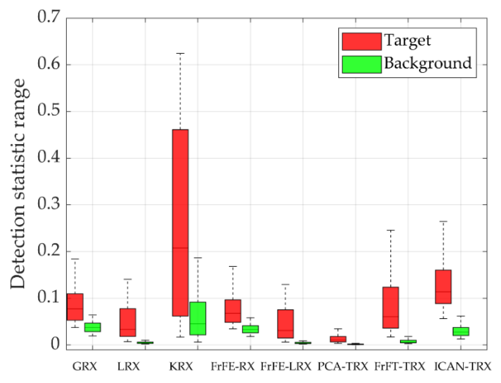
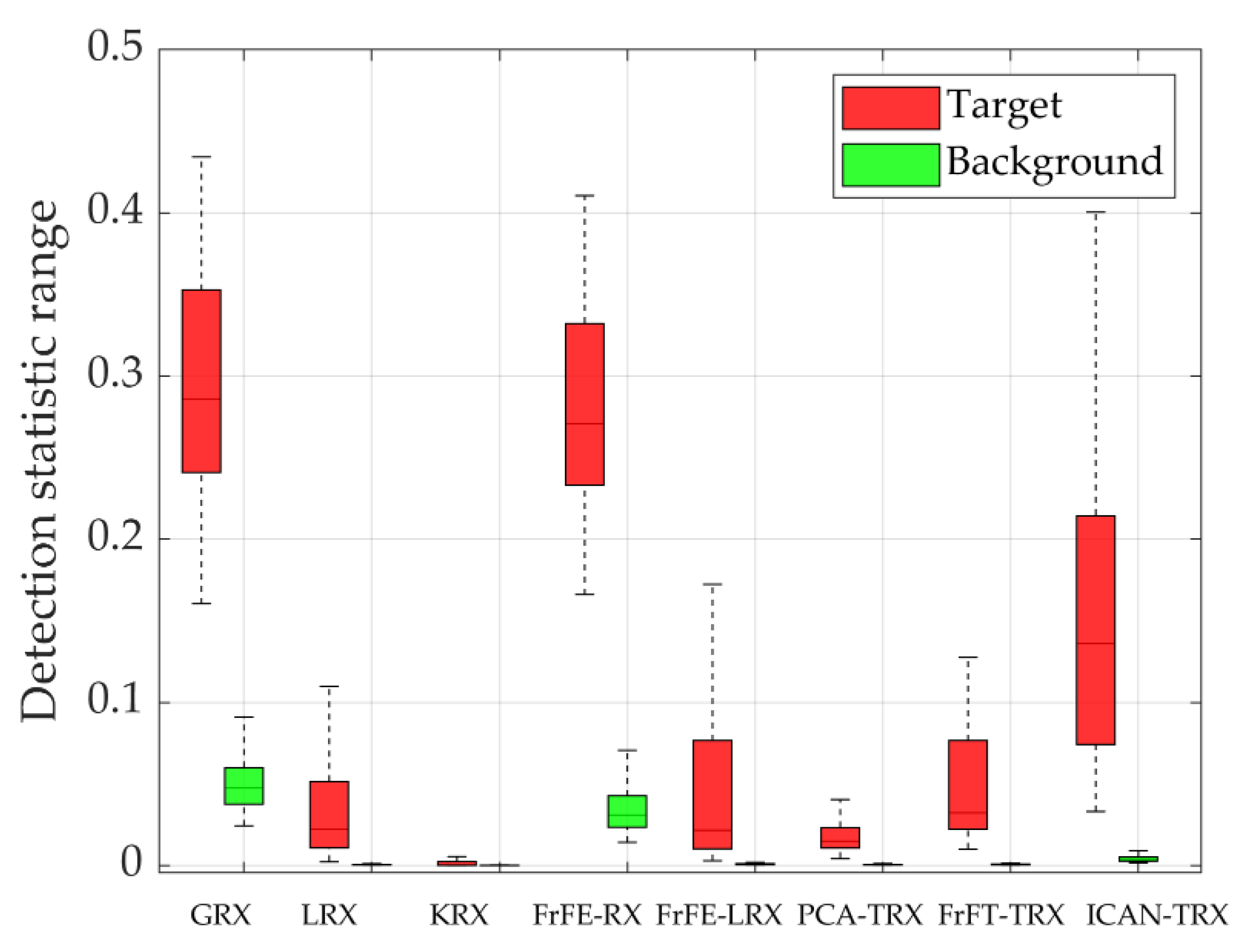
For the performance evaluation of the algorithms, this paper uses the two-dimensional diagrams of the AD results as the subjective evaluation, the receiver operating characteristic (ROC) curve, the area under the ROC curve (AUC), and the separability graph as the objective evaluation. For the separability graph in this paper, the highest and lowest 10% of the data are removed from each category.
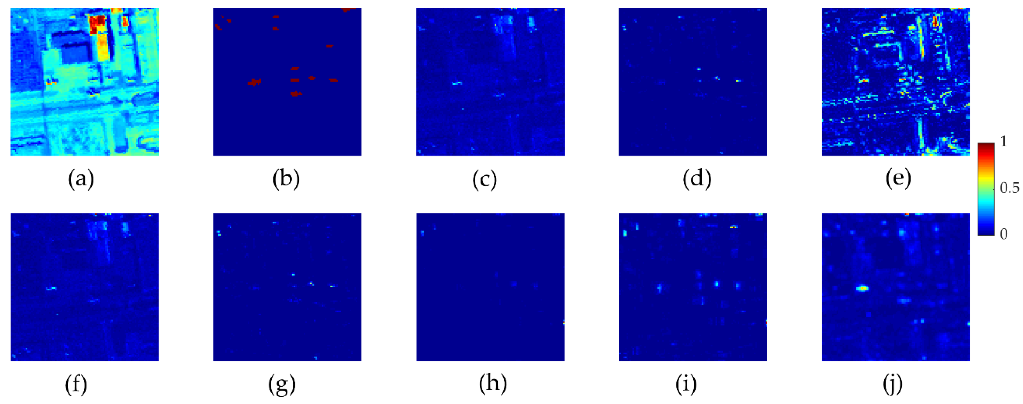
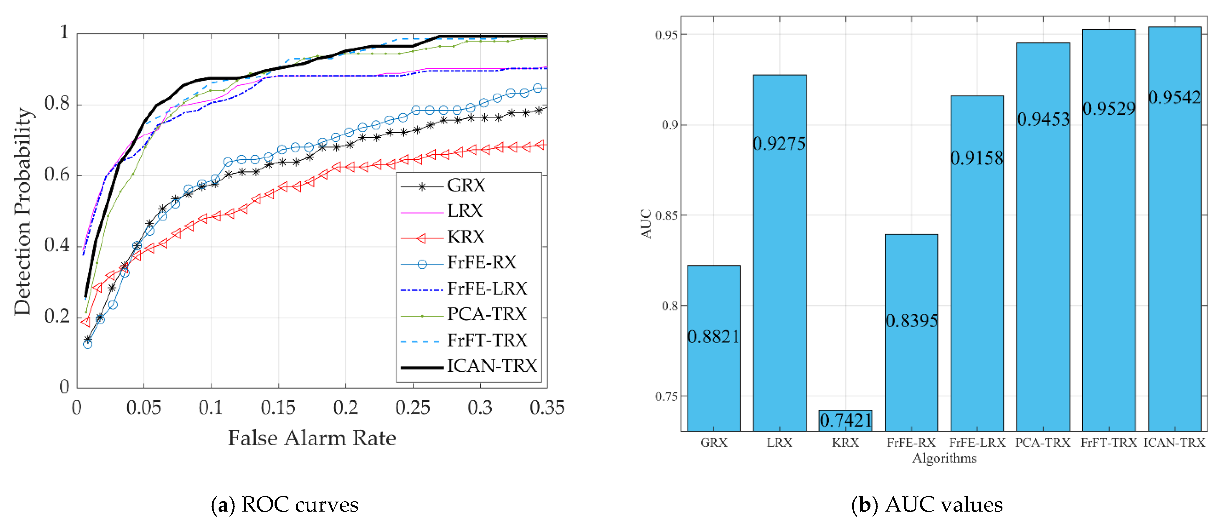
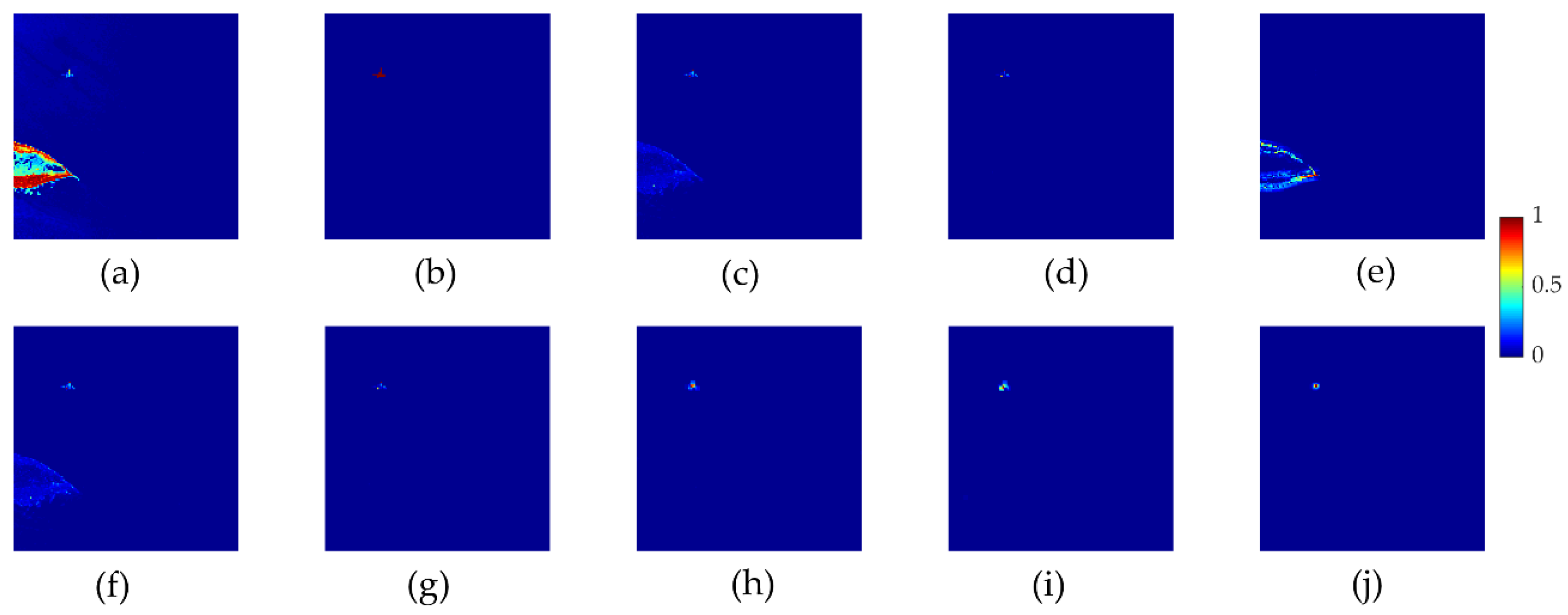
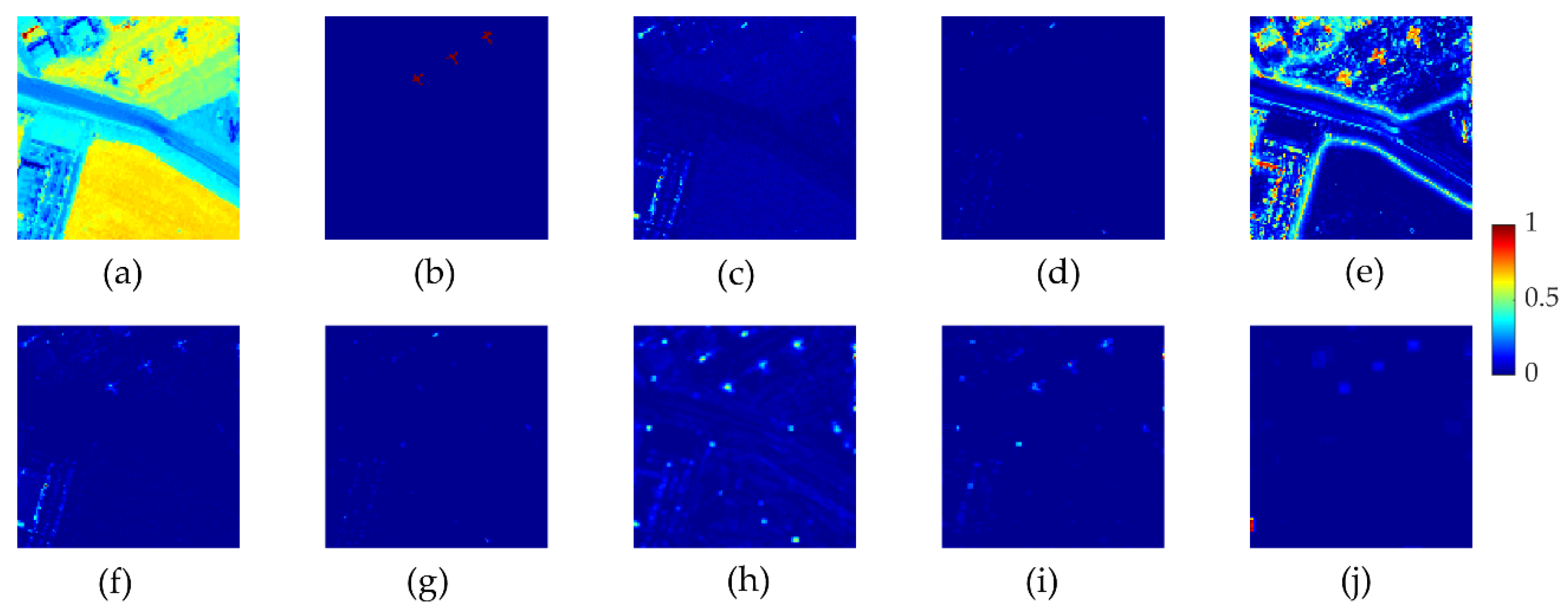
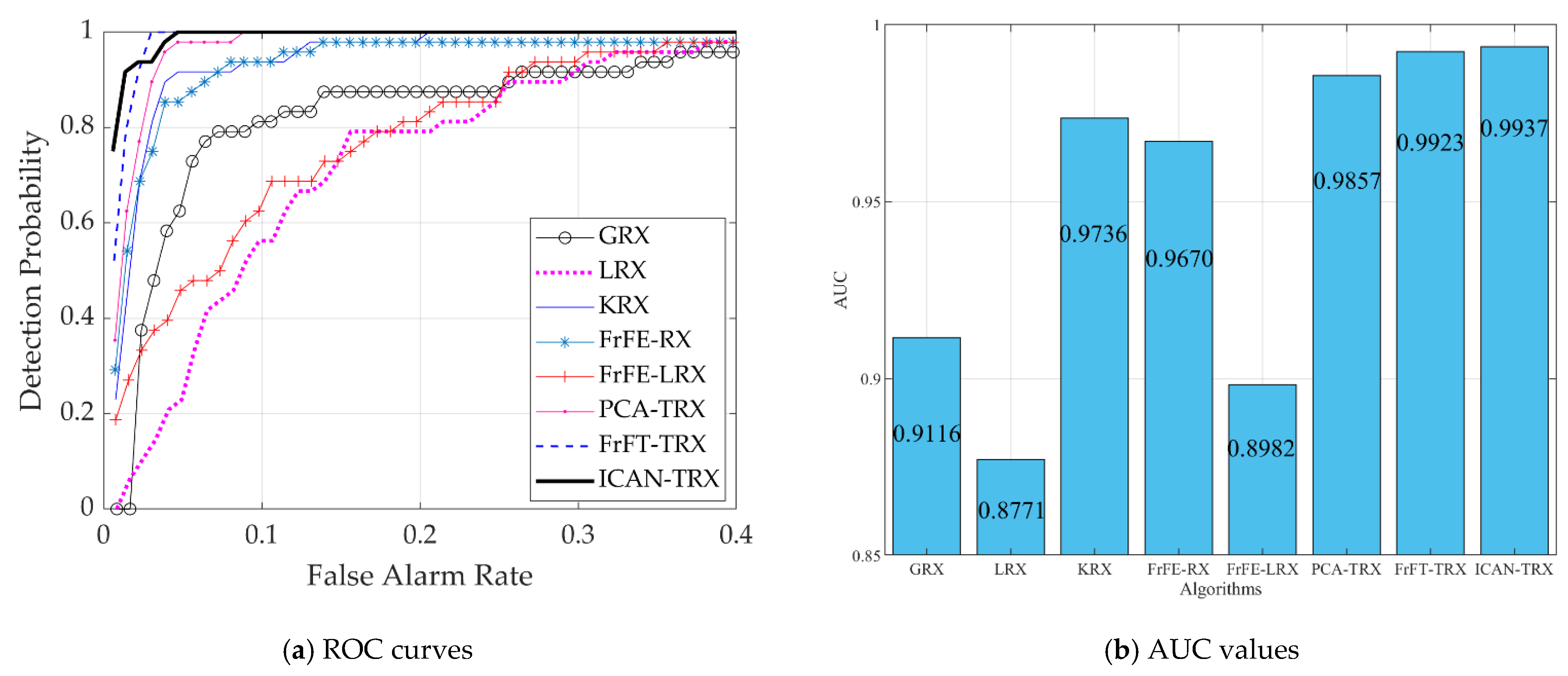
Figure 3 shows data L and two-dimensional diagrams of AD results for eight test algorithms. The anomaly targets in Figure 3j are more obvious than those in other comparison algorithms. Figure 4 shows the ROC curves and AUC values for data L. Figure 4a shows that the ROC curve of the proposed ICAN-TRX is superior to that of GRX, LRX, KRX, FrFE-RX, FrFE-LRX, and PCA-TRX, but close to that of FrFT-TRX. Combined with the AUC value in Figure 4b, it can be judged that the proposed ICAN-TRX algorithm has the best ROC curve and the largest AUC value. Figure 5 shows the separability graphs for data L. It can be seen that the distance between the target and the background of the ICAN-TRX algorithm is the largest among all the test algorithms, and its ability to compress the background is also acceptable.
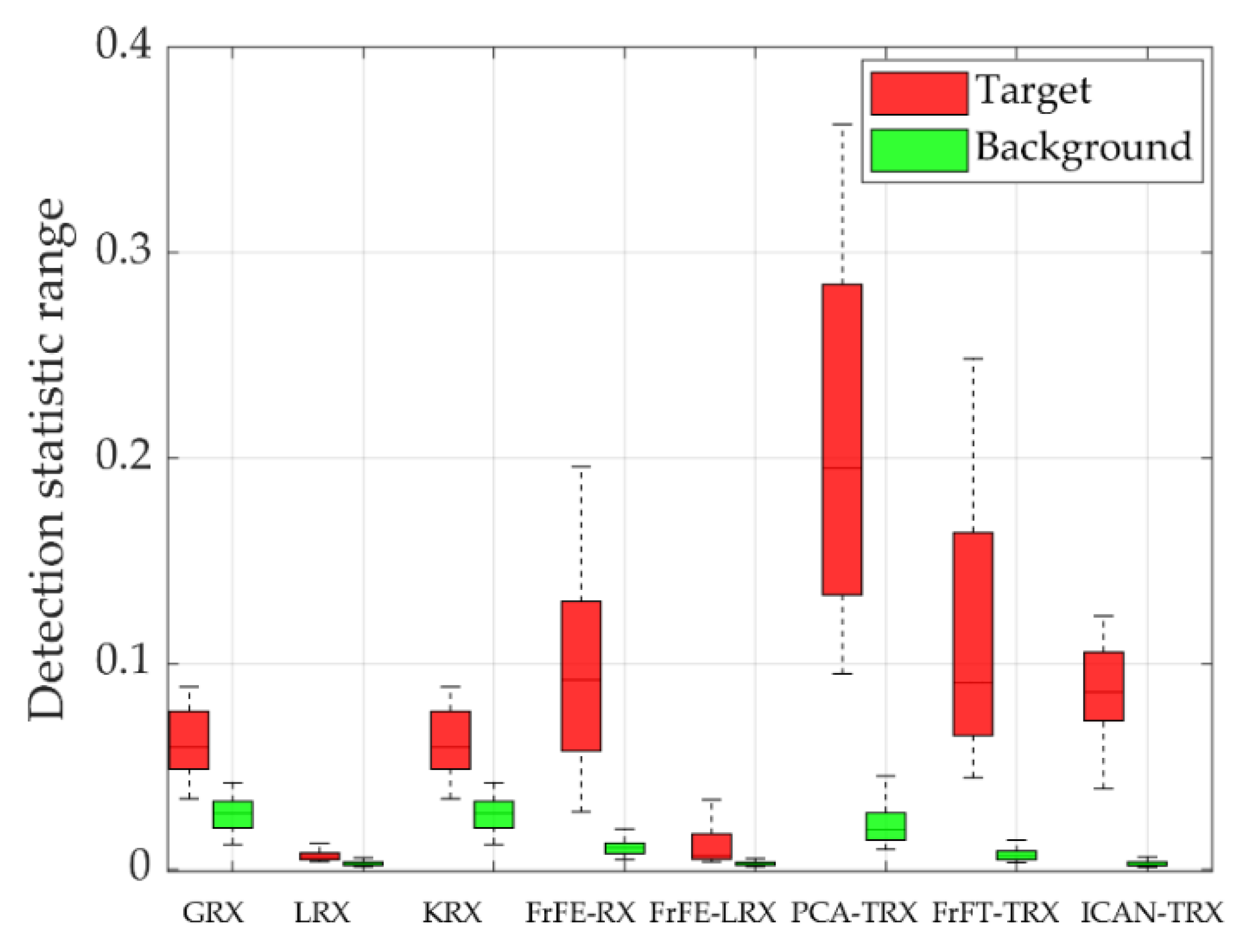
Figure 6 shows Data C and two-dimensional diagrams of AD results for eight test algorithms. From Figure 6, we can see that the anomaly targets in Figure 6h–j are more evident than those in the other five comparison algorithms. From Figure 7, it can be seen that the ROC curves and AUC values of FrFE-RX, FrFE-LRX, and FrFT-TRX are the same. Figure 8 shows the separability graphs for data C, and it can be judged that the distance between the target and the background of the ICAN-TRX algorithm is larger than LRX, KRX, and FrFE-LRX but less than GRX, FrFE-RX, PCA-TRX, and FrFT-TRX. However, the ability of ICAN-TRX to compress the background is slightly better than GRX, FrFE-RX, PCA-TRX, and FrFT-TRX.
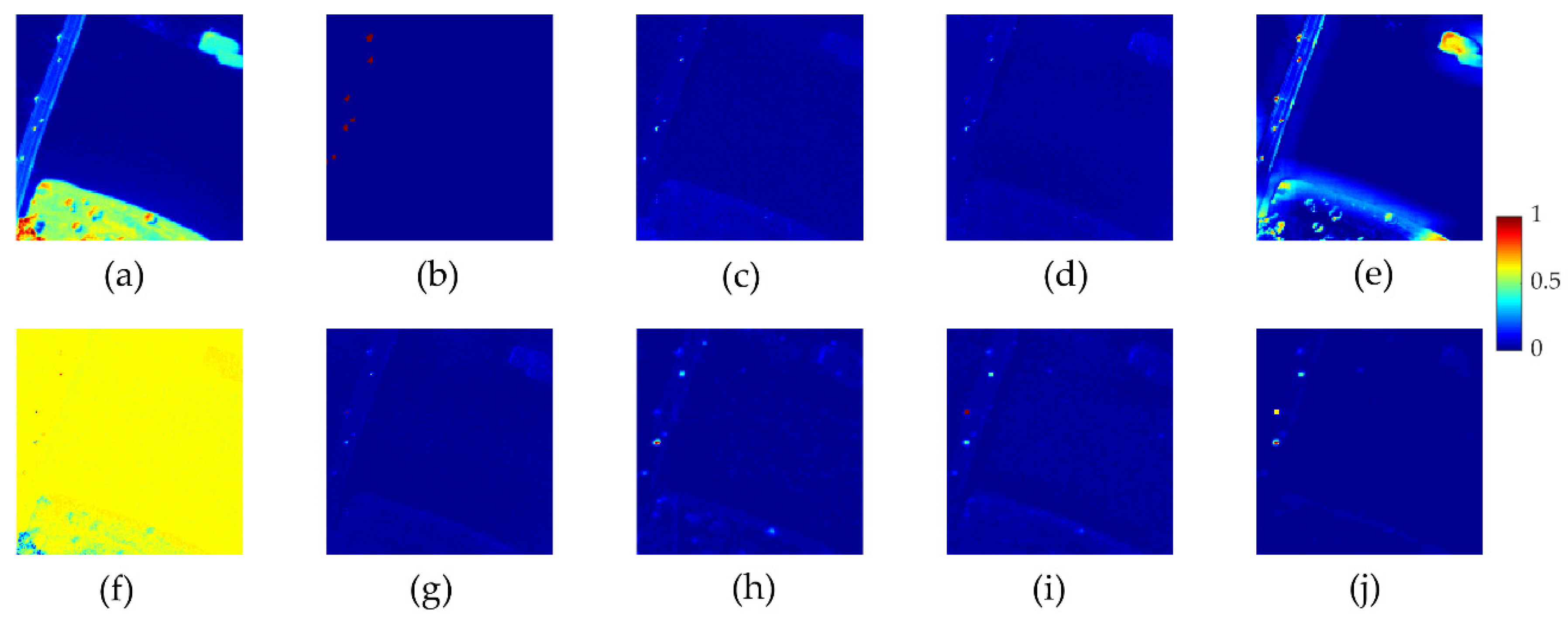
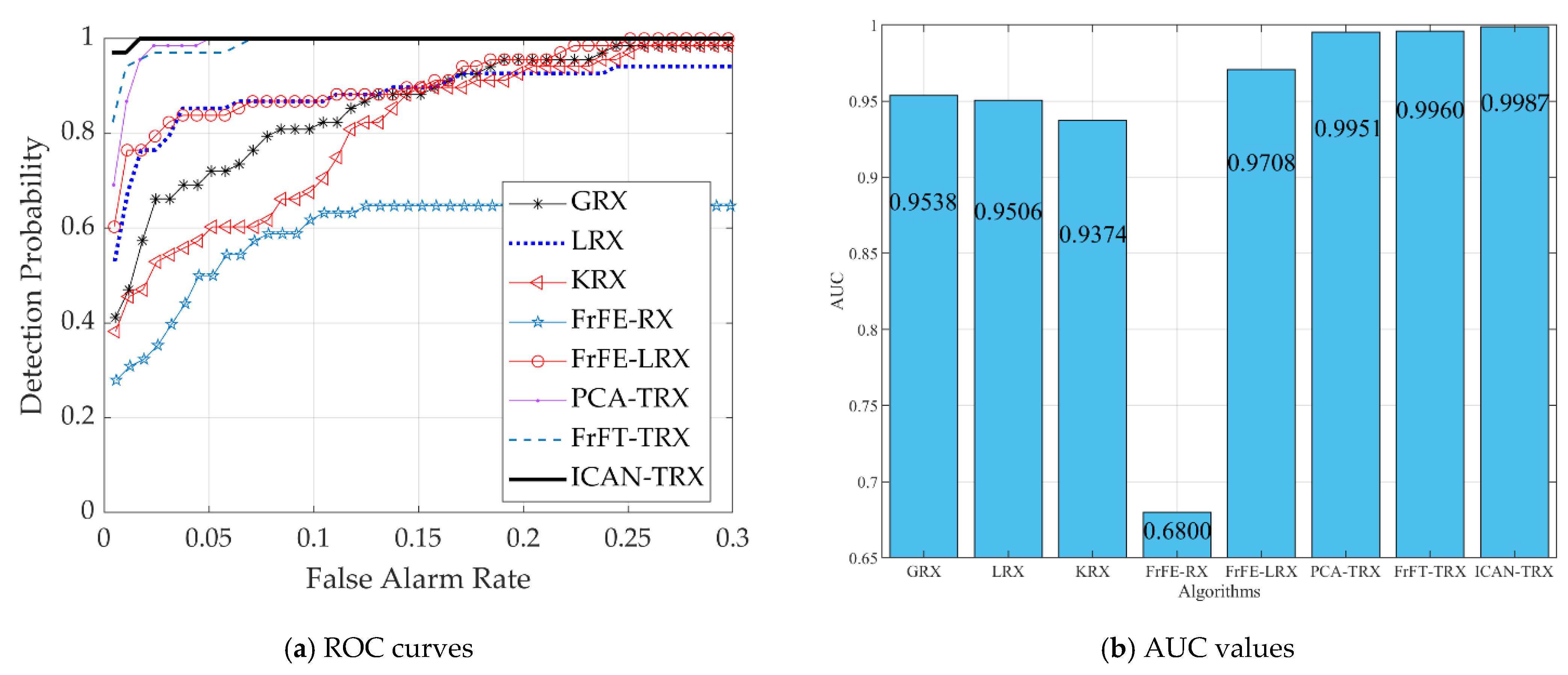
Figure 9 shows data P and two-dimensional diagrams of AD results for eight test algorithms. From Figure 9, we can find that the anomaly targets in Figure 9h–j are more striking than those in the other algorithms. The background in Figure 9j is more unitary than that in Figure 9h,i. It can be judged from Figure 10 that the proposed ICAN-TRX has the best ROC curve and the largest AUC value in the eight test algorithms. Figure 11 shows the separability graphs for data P. It can be judged that the distance between the target and the background of the ICAN-TRX algorithm is larger than GRX, KRX, FrFE-RX, and FrFE-LRX, and ICAN-TRX has the best ability to compress the background among all the test algorithms.
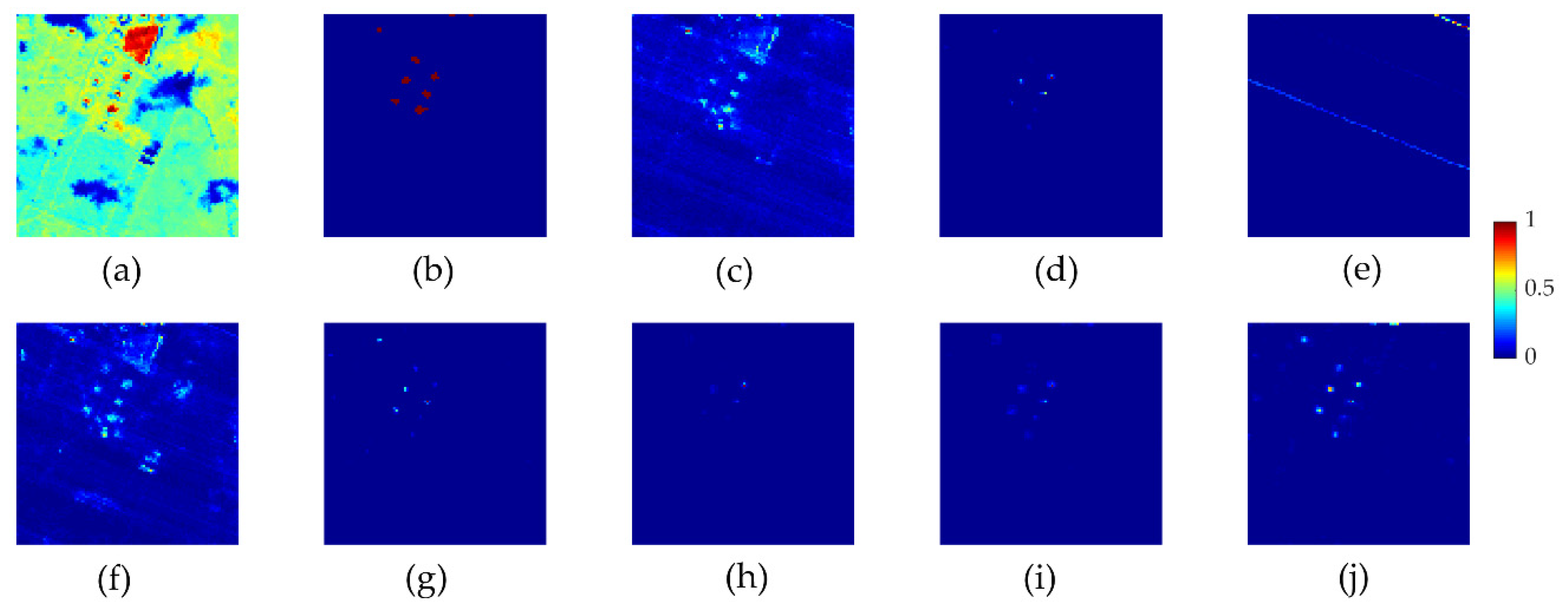
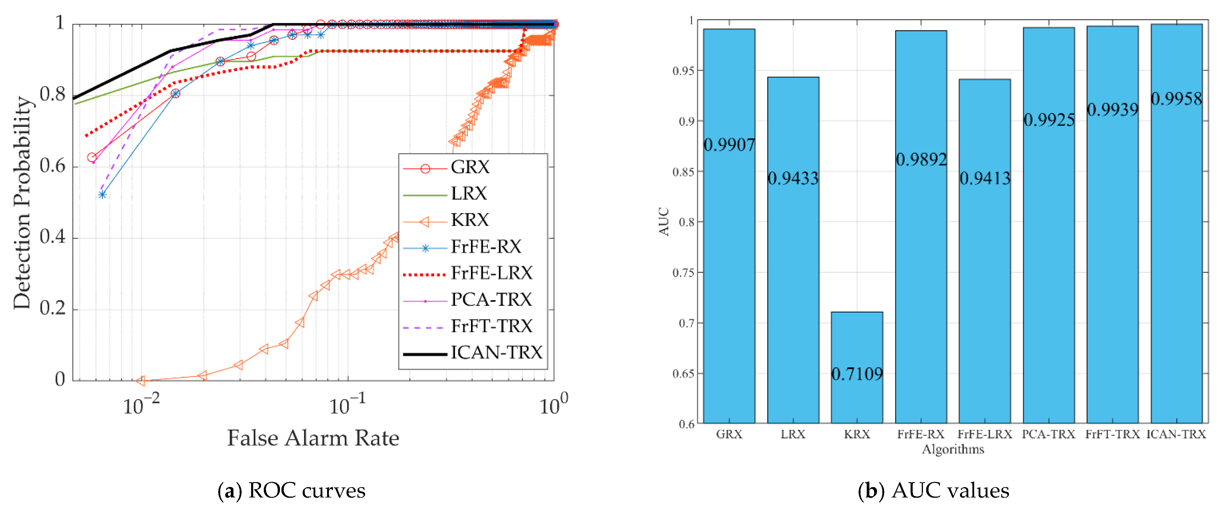
Figure 12 shows Data T and two-dimensional diagrams of AD results for eight test algorithms. As shown in Figure 12, the anomaly targets in Figure 12c,f,j are more evident than those in the other algorithms. However, some background points in Figure 12c,f are also evident. These background points are easily judged as anomaly targets, thus causing an increase in the false alarm rate. It can be judged from Figure 13 that the proposed ICAN-TRX has the best ROC curve and the largest AUC value in the eight test algorithms. As shown in Figure 14, the distance between the target and the background of the ICAN-TRX algorithm is larger than LRX, KRX, FrFE-LRX, PCA-TRX, and FrFT-TRX but smaller than GRX and FrFE-RX. However, the ability of ICAN-TRX to compress the background is better than GRX and FrFE-RX.
Figure 15 shows Data S and two-dimensional diagrams of AD results for eight test algorithms. As shown in Figure 15, the anomaly targets in Figure 15h–j are more evident than those in the other algorithms. However, some background points in Figure 15h,i are also evident and may be judged as anomaly targets, which causes an increase in the false alarm rate. From Figure 16, we can conclude that the proposed ICAN-TRX has the best ROC curve and the largest AUC value in the eight test algorithms. From Figure 17, we can see that the distance between the target and the background of the ICAN-TRX algorithm is larger than GRX, LRX, KRX, FrFE-RX, FrFE-LRX, and FrFT-TRX but smaller than PCA-TRX. However, the ability of ICAN-TRX to compress the background is better than PCA-TRX.
From the previous discussion and analysis, we can conclude that the detection performance of the proposed ICAN-TRX algorithm is generally better than that of the seven comparison algorithms. Table 3 lists the time consumption of the eight test algorithms for the five experimental HSIs. All experiments in this paper were completed by a computer with an Intel Core i7 CPU (central processing unit) and 16 GB of RAM (random-access memory). Matlab R2018b was used to implement the algorithm. The time consumption is not only related to the algorithm itself, but also the selection of parameters. From Table 3, we can see that the time consumption of ICAN-TRX is acceptable.
3.3. Parameter Analysis
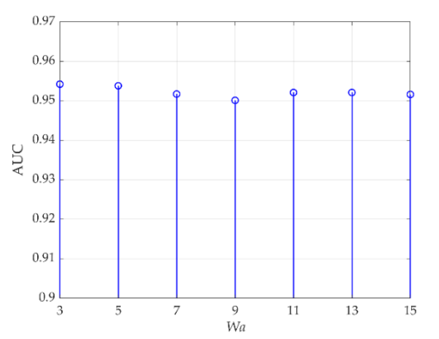
In the proposed ICAN-TRX algorithm, the changes in these three parameters, which are the spatial size Wa of the input tensor and the spatial sizes (Wt, Wb) of the target and background tensor, have a significant impact on the AD results. Compared with other parameters, the three parameters, ne, be, and le in DBNs, have very little impact on the AD results, so they are set to fixed values here, and will not be discussed. For data L, (ne, be, le) in the DBN reconstruction model are set to (10, 40, 2). First, Wa is set to 5, and AUC values changing with (Wt, Wb) are listed in Table 4. The optimal value is 0.9538 when (Wt, Wb) are set to (3, 41). Then, (Wt, Wb) is set to (3, 41), and AUC values changing with Wa are shown in Figure 18. When Wa is set to 3, the optimal AUC value 0.9542 is obtained.
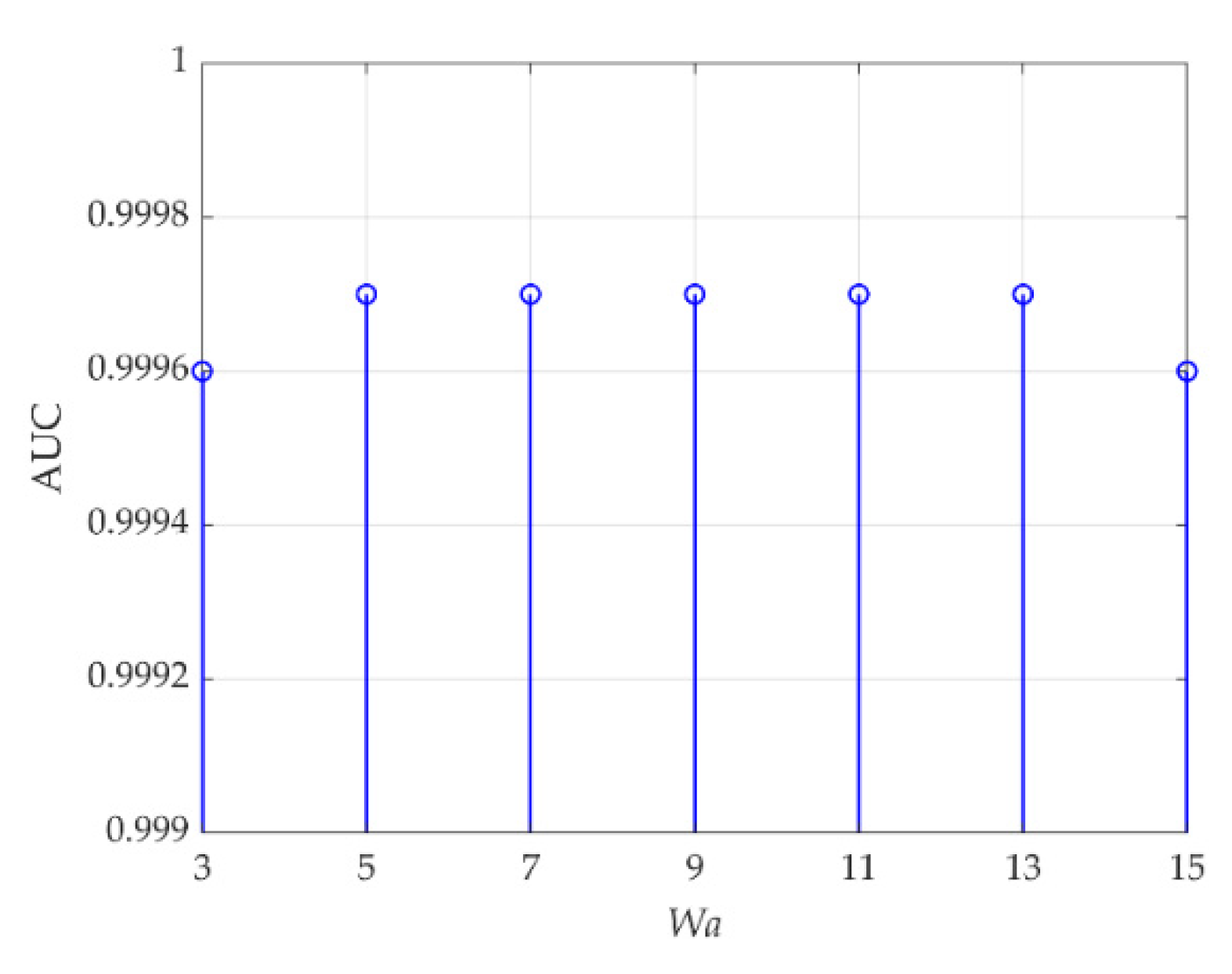
For data C, (ne, be, le) in the DBN reconstruction model are set to (6, 25, 2). The parameter Wa is first set to 5, and AUC values changing with (Wt, Wb) are shown in Table 5. The optimal value is 0.9997 when (Wt, Wb) are set to the dual-window sizes corresponding to bold values. Then, (Wt, Wb) is set to (5, 15), and Figure 19 reveals AUC values changing with Wa. When Wa is set to 5, 7, 9, 11, or 13, the optimal AUC value 0.9997 is obtained.
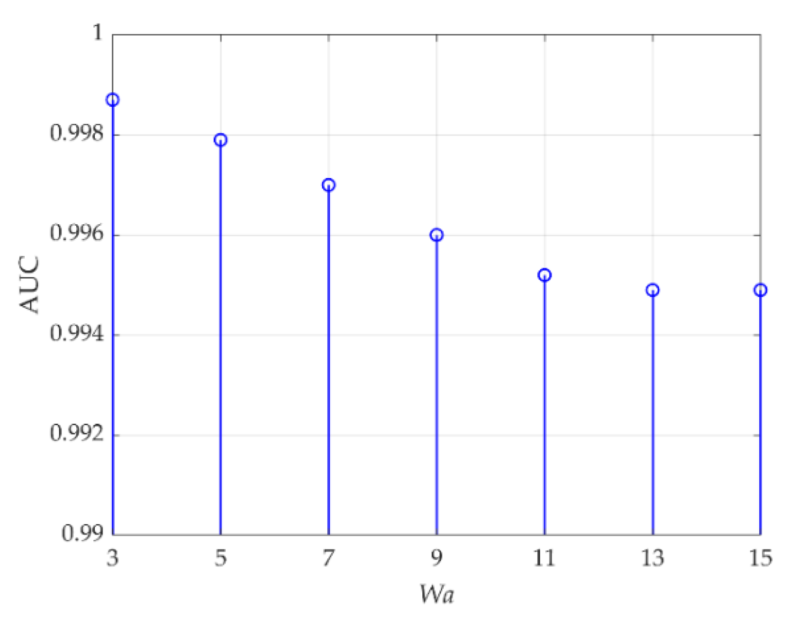
For data P, (ne, be, le) in the DBN reconstruction model are set to (10, 20, 2). The parameter Wa is first set to 5, and Table 6 reveals AUC values changing with (Wt, Wb). The optimal value is 0.9979 when (Wt, Wb) are set to (3, 35) or (3, 37). Then, (Wt, Wb) is set to (3, 35), and AUC values changing with Wa are shown in Figure 20. When Wa is set to 3, the optimal AUC value 0.9987 is obtained.
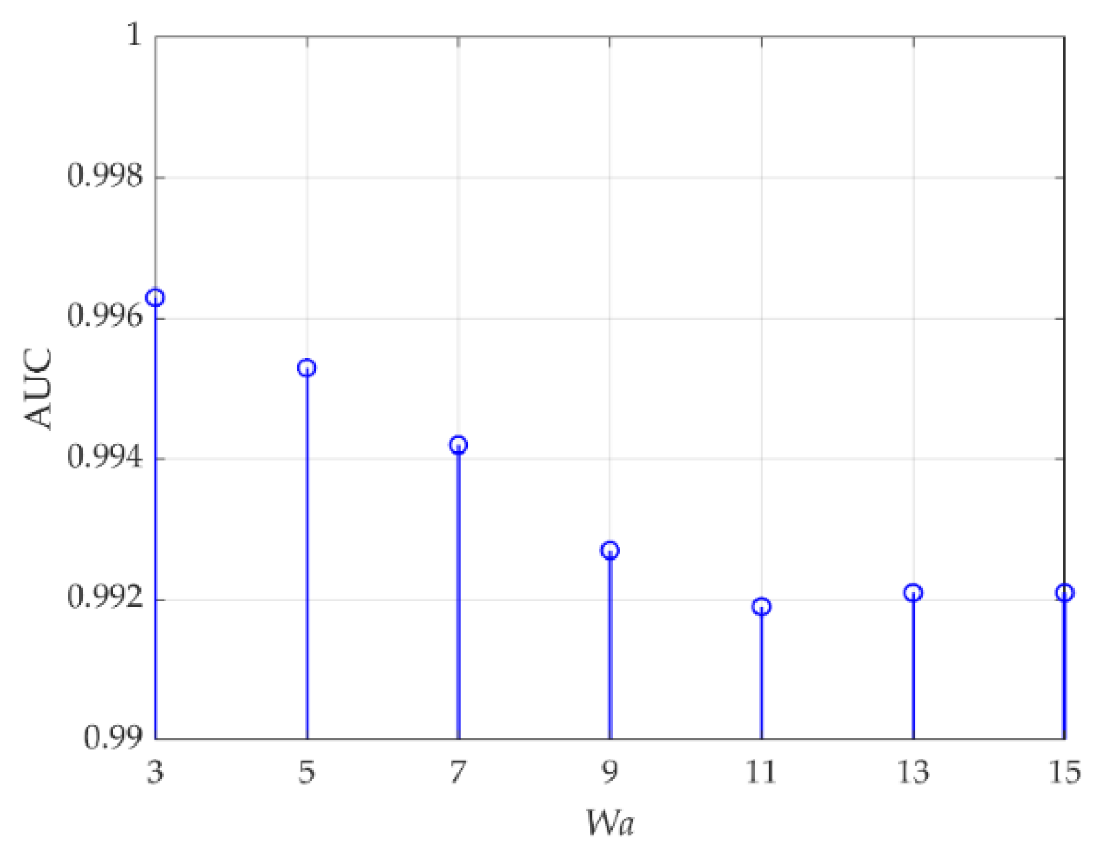
For data T, (ne, be, le) in the DBN reconstruction model are set to (10, 40, 2). The parameter Wa is first set to 5, and Table 7 reveals AUC values changing with (Wt, Wb). The optimal value is 0.9958 when (Wt, Wb) are set to (5, 9). Then, (Wt, Wb) is set to (5, 9), and AUC values changing with Wa are shown in Figure 21. When Wa is set to 3, the optimal AUC value 0.9963 is obtained.
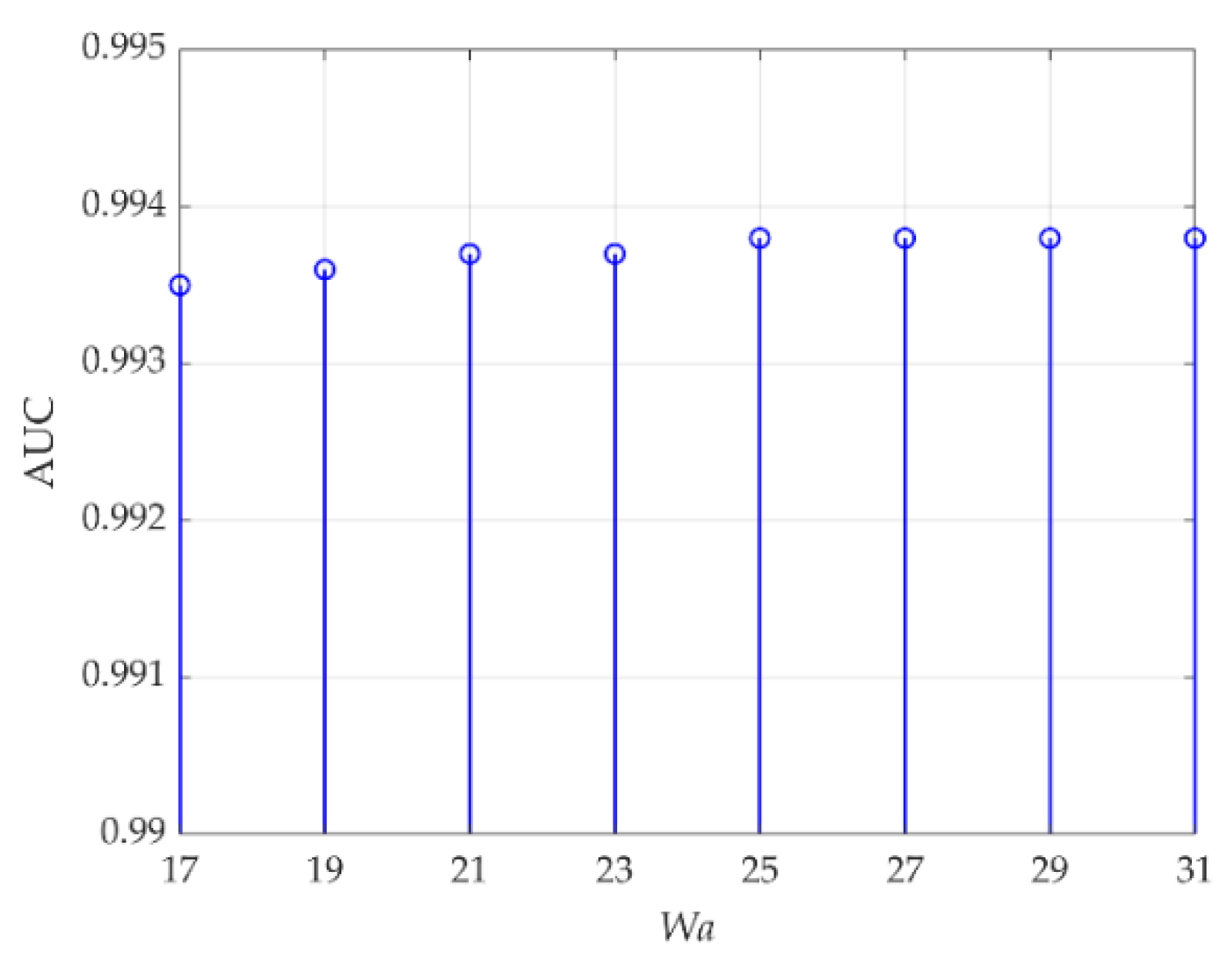
For data S, (ne, be, le) in the DBN reconstruction model are set to (5, 5, 2), respectively. The parameter Wa is first set to 21, and AUC values changing with (Wt, Wb) are listed in Table 8. The optimal value is 0.9937 when (Wt, Wb) are set to (11, 25). Then, (Wt, Wb) is set to (11, 25), and AUC values changing with Wa are shown in Figure 22. When Wa is set to 25, 27, 29, or 31, the optimal AUC value 0.9938 is obtained.
It can be seen from the above analysis that the values of the three parameters Wa, Wt, and Wb are directly related to the anomaly target sizes. In data L, data C, data P, and data T, the anomaly targets are all small, and the optimal values of Wa are 3 or 5. In data S, the anomaly targets are three aircraft whose sizes are relatively large, and the optimal value of Wa is 25, 27, 29, or 31. The optimal values of Wt and Wb in TRX are related to Wa and the characteristics of the experimental datasets, and they all need to be determined through repeated experiments.
4. Discussion
Hyperspectral AD mainly uses the spectral characteristics of HSIs, and spatial characteristics also play a crucial role in improving the detection results. In some AD algorithms using joint spectral–spatial characteristics, including tensor-based algorithms, all the neighboring pixels of a test point are treated equally without highlighting the test point. In the ICAN section of the proposed ICAN-TRX, the anomaly points in HSIs are more prominent through DBNs reconstruction, and the test point in the center of a test tensor block is used as a convolution kernel to perform convolution operation with the test tensor block. The spectral information of a test point is emphasized, and the similarity between the test point and its neighborhood points is also reflected. In TRX, more abundant spatial information is used, and the spatial sizes (Wt, Wb) of the target and background tensor are two important parameters affecting detection performance. In this paper, TRX is used after the ICAN, and the settings of Wt and Wb are also affected by the parameters of ICAN. In ICAN, the setting of the spatial size Wa of the input tensor is a crucial factor affecting the detection result and is mainly determined by the size of the anomaly target. However, there is no prior information for AD, so the setting of Wa is based on estimation and repeated experiments.
For data L, the optimal Wa and (Wt, Wb) are 3 and (3, 41), respectively. For data C, the optimal Wa is 5, 7, 9, 11, or 13, and the optimal (Wt, Wb) is (5, 15). For data P, the optimal Wa and (Wt, Wb) are 3 and (3, 35), respectively. For data T, the optimal Wa and (Wt, Wb) are 3 and (5, 9) respectively. For data S, the optimal Wa is 25, 27, 29, or 31 and the optimal (Wt, Wb) is (11, 25), respectively. For data L, C, P, and T, the values of Wa and Wt are equal or similar, and both are small sizes. This is mainly because the anomaly targets with small sizes contribute far less to the reconstruction of the DBN model than the background points. Through the DBNs reconstruction, the anomaly points in HSIs are more prominent, which is more conducive to AD. In data S, the sizes of anomaly targets are relatively large and not very sparse, so the contribution to DBNs reconstruction cannot be ignored. Some anomaly points may be considered as background points, which leads to a significant difference between the optimal Wa and Wt.
From the above discussion, we can see that the proposed algorithm requires more parameter adjustment for the detection of anomaly targets with large size and insufficient sparsity. To solve this problem, the DBNs reconstruction model should consider the spatial characteristics of anomaly targets, which may avoid reconstruction distortion. In addition, the adaptive selection of optimal parameters is the direction of improving the algorithm.
5. Conclusions
In some AD algorithms based on tensor, all the neighboring pixels of a test point in a tensor block are treated equally. Though the neighboring pixels provide spatial information, the spectral information of the test point should be the most important criterion. In this paper, an improved central attention network and tensor RX are combined for hyperspectral AD. In the section of ICAN, the anomaly points in HSIs are first more prominent through the DBNs reconstruction. Then, the spectral information of a test point in the center of the input tensor is emphasized. The similarity between the test point and its neighborhood points is also reflected through the convolution process. In the section of TRX, the spatial characteristics of the test point are used more comprehensively. The experimental verification on five real hyperspectral datasets shows that the overall detection performance of the proposed ICAN-TRX algorithm is better than that of the seven comparison algorithms. How to reasonably reserve the spatial characteristics of anomaly targets in the DBNs reconstruction model in the section of ICAN and adaptive selection of critical parameters are the subsequent work to improve the algorithm.
Author Contributions
Methodology, L.Z.; software, J.M.; validation, B.F. and F.L.; data curation, B.F.; writing—original draft preparation, L.Z. and J.M.; writing—review and editing, Y.S. and F.W.; funding acquisition, L.Z. All authors have read and agreed to the published version of the manuscript.
Funding
This research was funded by the National Natural Science Foundation of China under Grant (61901082), and Natural Science Foundation of Heilongjiang Province in China under Grant (LH2019F001).
Conflicts of Interest
The authors declare no conflict of interest.
References
- Plaza, A.; Benediktsson, J.A.; Boardman, J.W.; Brazile, J.; Bruzzone, L.; Camps-Valls, G.; Chanussot, J.; Fauvel, M.; Gamba, P.; Gualtieri, A.; et al. Recent Advances in Techniques for Hyperspectral Image Processing. Remote Sens. Environ. 2009, 113, S110–S122. [Google Scholar] [CrossRef]
- Landgrebe, D. Hyperspectral Image Data Analysis. IEEE Signal Process. Mag. 2002, 19, 17–28. [Google Scholar] [CrossRef]
- Cheng, G.; Han, J. A Survey on Object Detection in Optical Remote Sensing Images. ISPRS J. Photogramm. Remote Sens. 2016, 117, 11–28. [Google Scholar] [CrossRef] [Green Version]
- Yuan, Y.; Wang, Q.; Zhu, G. Fast Hyperspectral Anomaly Detection via High-Order 2-D Crossing Filter. IEEE Trans. Geosci. Remote Sens. 2015, 53, 620–630. [Google Scholar] [CrossRef]
- Ghamisi, P.; Yokoya, N.; Li, J.; Liao, W.; Liu, S.; Plaza, J.; Rasti, B.; Plaza, A. Advances in Hyperspectral Image and Signal Processing: A Comprehensive Overview of the State of the Art. IEEE Geosci. Remote Sens. Mag. 2017, 5, 37–78. [Google Scholar] [CrossRef] [Green Version]
- Chang, C.-I.; Chiang, S.-S. Anomaly Detection and Classification for Hyperspectral Imagery. IEEE Trans. Geosci. Remote Sens. 2002, 40, 1314–1325. [Google Scholar] [CrossRef] [Green Version]
- Matteoli, S.; Diani, M.; Corsini, G. A Tutorial Overview of Anomaly Detection in Hyperspectral Images. IEEE Aerosp. Electron. Syst. Mag. 2010, 25, 5–28. [Google Scholar] [CrossRef]
- Reed, I.S.; Yu, X. Adaptive Multiple-Band CFAR Detection of an Optical Pattern with Unknown Spectral Distribution. IEEE Trans. Acoust. 1990, 38, 1760–1770. [Google Scholar] [CrossRef]
- Molero, J.M.; Garzon, E.M.; Garcia, I.; Plaza, A. Analysis and Optimizations of Global and Local Versions of the RX Algorithm for Anomaly Detection in Hyperspectral Data. IEEE J. Sel. Top. Appl. Earth Obs. Remote. Sens. 2013, 6, 801–814. [Google Scholar] [CrossRef]
- Guo, Q.; Zhang, B.; Ran, Q.; Gao, L.; Li, J.; Plaza, A. Weighted-RXD and Linear Filter-Based RXD: Improving Background Statistics Estimation for Anomaly Detection in Hyperspectral Imagery. IEEE J. Sel. Top. Appl. Earth Obs. Remote. Sens. 2014, 7, 2351–2366. [Google Scholar] [CrossRef]
- Candes, E.J.; Romberg, J.; Tao, T. Robust Uncertainty Principles: Exact Signal Reconstruction from Highly Incomplete Frequency Information. IEEE Trans. Inf. Theory 2006, 52, 489–509. [Google Scholar] [CrossRef] [Green Version]
- Yuan, Z.Z.; Sun, H.; Ji, K.F.; Li, Z.Y.; Zou, H.X. Local Sparsity Divergence for Hyperspectral Anomaly Detection. IEEE Geosci. Remote Sens. Lett. 2014, 11, 1697–1701. [Google Scholar] [CrossRef]
- Li, W.; Du, Q. Collaborative Representation for Hyperspectral Anomaly Detection. IEEE Trans. Geosci. Remote Sens. 2015, 53, 1463–1474. [Google Scholar] [CrossRef]
- Li, J.; Zhang, H.; Zhang, L.; Ma, L. Hyperspectral Anomaly Detection by the Use of Background Joint Sparse Representation. IEEE J. Sel. Top. Appl. Earth Obs. Remote Sens. 2015, 8, 2523–2533. [Google Scholar] [CrossRef]
- Kang, X.; Xiang, X.; Li, S.; Benediktsson, J.A. PCA-Based Edge-Preserving Features for Hyperspectral Image Classification. IEEE Trans. Geosci. Remote Sens. 2017, 55, 7140–7151. [Google Scholar] [CrossRef]
- Meng, S.; Huang, L.-T.; Wang, W.-Q. Tensor Decomposition and PCA Jointed Algorithm for Hyperspectral Image Denoising. IEEE Geosci. Remote Sens. Lett. 2016, 13, 897–901. [Google Scholar] [CrossRef]
- Ma, L.; Crawford, M.M.; Tian, J. Anomaly Detection for Hyperspectral Images Based on Robust Locally Linear Embedding. J Infrared Millim. Terahertz Waves 2010, 31, 753–762. [Google Scholar] [CrossRef]
- Ma, L.; Crawford, M.M.; Tian, J. Anomaly Detection for Hyperspectral Images Using Local Tangent Space Alignment. In Proceedings of the IEEE International Geoscience and Remote Sensing Symposium, Honolulu, HI, USA, 25–30 July 2010; pp. 824–827. [Google Scholar]
- Zhang, L.; Zhao, C. Sparsity Divergence Index Based on Locally Linear Embedding for Hyperspectral Anomaly Detection. J. Appl. Remote Sens. 2016, 10, 025026. [Google Scholar] [CrossRef]
- Zhang, L.; Zhang, L.; Du, B. Deep Learning for Remote Sensing Data: A Technical Tutorial on the State of the Art. IEEE Geosci. Remote Sens. Mag. 2016, 4, 22–40. [Google Scholar] [CrossRef]
- Pan, B.; Shi, Z.; Xu, X. R-VCANet: A New Deep-Learning-Based Hyperspectral Image Classification Method. IEEE J. Sel. Top. Appl. Earth Obs. Remote Sens. 2018, 10, 1975–1986. [Google Scholar] [CrossRef]
- Hong, D.; Gao, L.; Yao, J.; Zhang, B.; Plaza, A.; Chanussot, J. Graph Convolutional Networks for Hyperspectral Image Classification. IEEE Trans. Geosci. Remote Sens. 2021, 59, 5966–5978. [Google Scholar] [CrossRef]
- Liu, P.; Zhang, H.; Eom, K.B. Active Deep Learning for Classification of Hyperspectral Images. IEEE J. Sel. Top. Appl. Earth Obs. Remote Sens. 2017, 10, 712–724. [Google Scholar] [CrossRef] [Green Version]
- Li, W.; Wu, G.; Du, Q. Transferred Deep Learning for Anomaly Detection in Hyperspectral Imagery. IEEE Geosci. Remote Sens. Lett. 2017, 14, 597–601. [Google Scholar] [CrossRef]
- Zhang, L.; Cheng, B. Transferred CNN Based on Tensor for Hyperspectral Anomaly Detection. IEEE Geosci. Remote Sens. Lett. 2020, 17, 2115–2119. [Google Scholar] [CrossRef]
- Tao, C.; Pan, H.; Li, Y.; Zou, Z. Unsupervised spectral–spatialfeature learning with stacked sparse autoencoder for hyperspectral imagery classification. IEEE Geosci. Remote Sens. Lett. 2015, 12, 2438–2442. [Google Scholar] [CrossRef]
- Ma, X.; Wang, H.; Geng, J. Spectral–Spatial Classification of Hyperspectral Image Based on Deep Auto-Encoder. IEEE J. Sel. Top. Appl. Earth Obs. Remote Sens. 2016, 9, 4073–4085. [Google Scholar] [CrossRef]
- Chen, Y.; Lin, Z.; Zhao, X.; Wang, G.; Gu, Y. Deep Learning-Based Classification of Hyperspectral Data. IEEE J. Sel. Top. Appl. Earth Obs. Remote Sens. 2014, 7, 2094–2107. [Google Scholar] [CrossRef]
- Chen, Y.; Zhao, X.; Jia, X. Spectral–Spatial Classification of Hyperspectral Data Based on Deep Belief Network. IEEE J. Sel. Top. Appl. Earth Obs. Remote Sens. 2015, 8, 2381–2392. [Google Scholar] [CrossRef]
- Zhang, L.; Cheng, B. A Stacked Autoencoders-Based Adaptive Subspace Model for Hyperspectral Anomaly Detection. Infrared Phys. Technol. 2019, 96, 52–60. [Google Scholar] [CrossRef]
- Zhang, L.; Cheng, B.; Lin, F. Hyperspectral Anomaly Detection via Fractional Fourier Transform and Deep Belief Networks. Infrared Phys. Technol. 2022, 125, 104314. [Google Scholar] [CrossRef]
- Plaza, A.; Martín, G.; Plaza, J.; Zortea, M.; Sánchez, S. Recent Developments in Endmember Extraction and Spectral Unmixing. In Optical Remote Sensing; Springer: Berlin/Heidelberg, Germany, 2011; pp. 235–267. [Google Scholar]
- Zhang, L.; Zhao, C. A Spectral-Spatial Method Based on Low-Rank and Sparse Matrix Decomposition for Hyperspectral Anomaly Detection. Int. J. Remote Sens. 2017, 38, 4047–4068. [Google Scholar] [CrossRef]
- Du, B.; Zhao, R.; Zhang, L.; Zhang, L. A Spectral-Spatial Based Local Summation Anomaly Detection Method for Hyperspectral Images. Signal Process. 2016, 124, 115–131. [Google Scholar] [CrossRef]
- Lin, T.; Bourennane, S. Survey of Hyperspectral Image Denoising Methods Based on Tensor Decompositions. EURASIP J. Adv. Signal Process. 2013, 2013, 186. [Google Scholar] [CrossRef] [Green Version]
- Geng, X.; Sun, K.; Ji, L.; Zhao, Y. A High-Order Statistical Tensor Based Algorithm for Anomaly Detection in Hyperspectral Imagery. Sci. Rep. 2015, 4, 6869. [Google Scholar] [CrossRef] [PubMed] [Green Version]
- Li, S.; Wang, W.; Qi, H.; Ayhan, B.; Kwan, C.; Vance, S. Low-Rank Tensor Decomposition Based Anomaly Detection for Hyperspectral Imagery. In Proceedings of the IEEE International Conference on Image Processing (ICIP), Quebec City, QC, Canada, 27–30 September 2015; pp. 4525–4529. [Google Scholar]
- Zhang, X.; Wen, G.; Dai, W. A Tensor Decomposition-Based Anomaly Detection Algorithm for Hyperspectral Image. IEEE Trans. Geosci. Remote Sens. 2016, 54, 5801–5820. [Google Scholar] [CrossRef]
- Capobianco, L.; Garzelli, A.; Camps-Valls, G. Target Detection with Semisupervised Kernel Orthogonal Subspace Projection. IEEE Trans. Geosci. Remote Sens. 2009, 47, 3822–3833. [Google Scholar] [CrossRef]
- Harsanyi, J.; Chang, C. Hyperspectral image classification and dimensionality reduction: An orthogonal subspace projection approach. IEEE Trans. Geosci. Remote Sens. 1994, 32, 779–785. [Google Scholar] [CrossRef] [Green Version]
- Zhang, L.; Cheng, B.; Deng, Y. A Tensor-Based Adaptive Subspace Detector for Hyperspectral Anomaly Detection. Int. J. Remote Sens. 2018, 39, 2366–2382. [Google Scholar] [CrossRef]
- Zhang, L.; Ma, J.; Cheng, B.; Lin, F. Fractional Fourier Transform Based Tensor RX for Hyperspectral Anomaly Detection. Remote Sens. 2022, 14, 797. [Google Scholar] [CrossRef]
- He, J.; Zhao, L.; Yang, H.; Zhang, M.; Li, W. HSI-BERT: Hyperspectral Image Classification Using the Bidirectional Encoder Representation from Transformers. IEEE Trans. Geosci. Remote Sens. 2020, 58, 165–178. [Google Scholar] [CrossRef]
- Pu, C.; Huang, H.; Yang, L. An Attention-Driven Convolutional Neural Network-Based Multi-Level Spectral–Spatial Feature Learning for Hyperspectral Image Classification. Expert Syst. Appl. 2021, 185, 115663. [Google Scholar] [CrossRef]
- Liu, H.; Li, W.; Xia, X.-G.; Zhang, M.; Gao, C.-Z.; Tao, R. Central Attention Network for Hyperspectral Imagery Classification. IEEE Trans. Neural Netw. Learn. Syst. 2022, 185, 1–15. [Google Scholar] [CrossRef] [PubMed]
- Liu, J.; Hou, Z.; Li, W.; Tao, R.; Orlando, D.; Li, H. Multipixel Anomaly Detection with Unknown Patterns for Hyperspectral Imagery. IEEE Trans. Neural Netw. Learn. Syst. 2022, 33, 5557–5567. [Google Scholar] [CrossRef] [PubMed]
- Horn, R.A.; Johnson, C.R. Matrix Analysis; Cambridge University Press: Cambridge, UK, 1985; p. 176. [Google Scholar]
- Kang, X.; Zhang, X.; Li, S.; Li, K.; Li, J.; Benediktsson, J.A. Hyperspectral Anomaly Detection with Attribute and Edge-Preserving Filters. IEEE Trans. Geosci. Remote Sens. 2017, 55, 5600–5611. [Google Scholar] [CrossRef]
Figure 1.
Graphical representation of DBNs.

Figure 2.
A diagram of ICAN.

Figure 3.
Data L and AD result diagrams: (a) The 100th band of data L. (b) The ground-truth map. (c) GRX. (d) LRX. (e) KRX. (f) FrFE-RX. (g) FrFE-LRX. (h) PCA-TRX. (i) FrFT-TRX. (j) ICAN-TRX.
Figure 3.
Data L and AD result diagrams: (a) The 100th band of data L. (b) The ground-truth map. (c) GRX. (d) LRX. (e) KRX. (f) FrFE-RX. (g) FrFE-LRX. (h) PCA-TRX. (i) FrFT-TRX. (j) ICAN-TRX.

Figure 4.
ROC curves and AUC values for data L.

Figure 5.
Separability graphs for data L.

Figure 6.
Data C and AD result diagrams: (a) The 100th band of data C. (b) The ground-truth map. (c) GRX. (d) LRX. (e) KRX. (f) FrFE-RX. (g) FrFE-LRX. (h) PCA-TRX. (i) FrFT-TRX. (j) ICAN-TRX.
Figure 6.
Data C and AD result diagrams: (a) The 100th band of data C. (b) The ground-truth map. (c) GRX. (d) LRX. (e) KRX. (f) FrFE-RX. (g) FrFE-LRX. (h) PCA-TRX. (i) FrFT-TRX. (j) ICAN-TRX.

Figure 7.
ROC curves and AUC values for data C.

Figure 8.
Separability graphs for data C.

Figure 9.
Data P and AD result diagrams: (a) The 100th band of data C. (b) The ground-truth map. (c) GRX. (d) LRX. (e) KRX. (f) FrFE-RX. (g) FrFE-LRX. (h) PCA-TRX. (i) FrFT-TRX. (j) ICAN-TRX.
Figure 9.
Data P and AD result diagrams: (a) The 100th band of data C. (b) The ground-truth map. (c) GRX. (d) LRX. (e) KRX. (f) FrFE-RX. (g) FrFE-LRX. (h) PCA-TRX. (i) FrFT-TRX. (j) ICAN-TRX.

Figure 10.
ROC curves and AUC values for data P.

Figure 11.
Separability graphs for data P.

Figure 12.
Data T and AD result diagrams: (a) The 100th band of data C. (b) The ground-truth map. (c) GRX. (d) LRX. (e) KRX. (f) FrFE-RX. (g) FrFE-LRX. (h) PCA-TRX. (i) FrFT-TRX. (j) ICAN-TRX.
Figure 12.
Data T and AD result diagrams: (a) The 100th band of data C. (b) The ground-truth map. (c) GRX. (d) LRX. (e) KRX. (f) FrFE-RX. (g) FrFE-LRX. (h) PCA-TRX. (i) FrFT-TRX. (j) ICAN-TRX.

Figure 13.
ROC curves and AUC values for data T.

Figure 14.
Separability graphs for data T.

Figure 15.
Data S and AD result diagrams: (a) The 100th band of data C. (b) The ground-truth map. (c) GRX. (d) LRX. (e) KRX. (f) FrFE-RX. (g) FrFE-LRX. (h) PCA-TRX. (i) FrFT-TRX. (j) ICAN-TRX.
Figure 15.
Data S and AD result diagrams: (a) The 100th band of data C. (b) The ground-truth map. (c) GRX. (d) LRX. (e) KRX. (f) FrFE-RX. (g) FrFE-LRX. (h) PCA-TRX. (i) FrFT-TRX. (j) ICAN-TRX.

Figure 16.
ROC curves and AUC values for data S.

Figure 17.
Separability graphs for data S.

Figure 18.
AUC values changing with Wa for data L.

Figure 19.
AUC values changing with Wa for data C.

Figure 20.
AUC values changing with Wa for data P.

Figure 21.
AUC values changing with Wa for data T.

Figure 22.
AUC values changing with Wa for data S.


Table 1.
Relevant data of five experimental HSIs.
| Data | Captured Place | Resolution | Sensor | Experimental Size | Fight Time |
|---|---|---|---|---|---|
| Data L | Los Angeles | 7.1 m | AVIRIS | 100 × 100 × 205 | 11/9/2011 |
| Data C | Cat Island | 17.2 m | AVIRIS | 150 × 150 × 189 | 9/12/2010 |
| Data P | Pavia | 1.3 m | ROSIS-03 | 150 × 150 × 102 | Unknown |
| Data T | Texas Coast | 17.2 m | AVIRIS | 100 × 100 × 204 | 8/29/2010 |
| Data S | San Diego | 3.5 m | AVIRIS | 120 × 120 × 126 | Unkown |
Table 2.
Parameter settings of LRX, KRX, FrFE-RX, FrFE-LRX, PCA-TRX, FrFT-TRX, and ICAN-TRX for the five experimental HSIs.
Table 2.
Parameter settings of LRX, KRX, FrFE-RX, FrFE-LRX, PCA-TRX, FrFT-TRX, and ICAN-TRX for the five experimental HSIs.
| Data | LRX (Win, Wout) | KRX (c,Win, Wout) | FrFE-RX p | FrFE-LRX (p, Win, Wout) | PCA-TRX (d, Wt, Wb) | FrFT-TRX (p, Wt, Wb) | ICAN-TRX (Wa, Wt, Wb) (ne, be, le) |
|---|---|---|---|---|---|---|---|
| Data L | (7, 9) | (10−5, 5, 9) | 0.2 | (0.2, 7, 9) | (10, 7, 9) | (1, 7, 9) | (3, 3, 41) (10, 40, 2) |
| Data C | (25, 77) | (10−2, 5, 7) | 0.2 | (0.2, 25, 77) | (10, 3, 37) | (0.2, 3, 37) | (5, 5, 15) (6, 25, 2) |
| Data P | (25, 81) | (10−1, 25, 29) | 1 | (1, 25, 77) | (20, 3, 37) | (1, 3, 37) | (3, 3, 35) (10, 20, 2) |
| Data T | (7, 9) | (10−2, 7, 9) | 1 | (1, 5, 7) | (8, 7, 9) | (0.2, 7, 9) | (5, 5, 9) (10, 40, 2) |
| Data S | (7, 9) | (10−2, 7, 9) | 0.9 | (0.9, 7, 9) | (9, 3, 31) | (0.9, 3, 31) | (21, 11, 25) (5, 5, 2) |
Table 3.
Time consumption (in seconds) of eight test algorithms for the five HSIs.
| Data | GRX | LRX | KRX | FrFE-RX | FrFE-LRX | PCA-TRX | FrFT-TRX | ICAN-TRX |
|---|---|---|---|---|---|---|---|---|
| Data L | 1.43 | 27.79 | 56.67 | 11.35 | 39.08 | 4.97 | 32.54 | 88.46 |
| Data C | 0.71 | 421.21 | 25.87 | 22.35 | 430.72 | 2.92 | 140.65 | 70.36 |
| Data P | 0.63 | 236.19 | 1418.01 | 11.86 | 218.95 | 5.56 | 44.78 | 39.36 |
| Data T | 0.58 | 26.95 | 20.92 | 10.96 | 38.06 | 5.64 | 33.13 | 33.80 |
| Data S | 0.59 | 15.05 | 26.21 | 9.37 | 24.89 | 1.80 | 33.61 | 75.66 |
Table 4.
AUC values changing with (Wt, Wb) for data L.
| Wt | Wb | |||||||
|---|---|---|---|---|---|---|---|---|
| 33 | 35 | 37 | 39 | 41 | 43 | 45 | 47 | |
| 3 | 0.9527 | 0.9530 | 0.9507 | 0.9529 | 0.9538 | 0.9531 | 0.9487 | 0.9436 |
| 5 | 0.9274 | 0.9298 | 0.9263 | 0.9304 | 0.9307 | 0.928 | 0.9207 | 0.9129 |
| 7 | 0.8746 | 0.8782 | 0.8814 | 0.8787 | 0.8815 | 0.8752 | 0.8629 | 0.8488 |
Table 5.
AUC values changing with (Wt, Wb) for data C.
| Wt | Wb | |||||||
|---|---|---|---|---|---|---|---|---|
| 11 | 13 | 15 | 17 | 19 | 21 | 23 | 25 | |
| 3 | 0.9994 | 0.9996 | 0.9997 | 0.9997 | 0.9997 | 0.9997 | 0.9996 | 0.9996 |
| 5 | 0.9995 | 0.9996 | 0.9997 | 0.9997 | 0.9997 | 0.9997 | 0.9996 | 0.9996 |
| 7 | 0.9995 | 0.9995 | 0.9996 | 0.9996 | 0.9996 | 0.9996 | 0.9996 | 0.9995 |
Table 6.
AUC values changing with (Wt, Wb) for data P.
| Wt | Wb | |||||||
|---|---|---|---|---|---|---|---|---|
| 33 | 35 | 37 | 39 | 41 | 43 | 45 | 47 | |
| 3 | 0.9977 | 0.9979 | 0.9979 | 0.9968 | 0.9959 | 0.9955 | 0.9956 | 0.9953 |
| 5 | 0.9959 | 0.9958 | 0.9954 | 0.9945 | 0.9934 | 0.9933 | 0.9932 | 0.9928 |
| 7 | 0.9915 | 0.9915 | 0.9912 | 0.9897 | 0.9885 | 0.9871 | 0.9872 | 0.9965 |
Table 7.
AUC values changing with (Wt, Wb) for data T.
| Wt | Wb | ||||
|---|---|---|---|---|---|
| 9 | 11 | 13 | 15 | 17 | |
| 3 | 0.9812 | 0.9839 | 0.9856 | 0.9798 | 0.9774 |
| 5 | 0.9958 | 0.9930 | 0.9882 | 0.9750 | 0.9648 |
| 7 | 0.9926 | 0.9911 | 0.9785 | 0.9650 | 0.9351 |
Table 8.
AUC values changing with (Wt, Wb) for data S.
| Wt | Wb | |||||
|---|---|---|---|---|---|---|
| 19 | 21 | 23 | 25 | 27 | 29 | |
| 9 | 0.9679 | 0.9777 | 0.9841 | 0.9875 | 0.9894 | 0.9888 |
| 11 | 0.9868 | 0.9907 | 0.9926 | 0.9937 | 0.9933 | 0.9910 |
| 13 | 0.9888 | 0.9915 | 0.9933 | 0.9934 | 0.9923 | 0.9869 |
Publisher’s Note: MDPI stays neutral with regard to jurisdictional claims in published maps and institutional affiliations. |
© 2022 by the authors. Licensee MDPI, Basel, Switzerland. This article is an open access article distributed under the terms and conditions of the Creative Commons Attribution (CC BY) license (https://creativecommons.org/licenses/by/4.0/).
Share and Cite
MDPI and ACS Style
Zhang, L.; Ma, J.; Fu, B.; Lin, F.; Sun, Y.; Wang, F. Improved Central Attention Network-Based Tensor RX for Hyperspectral Anomaly Detection. Remote Sens. 2022, 14, 5865. https://doi.org/10.3390/rs14225865
AMA Style
Zhang L, Ma J, Fu B, Lin F, Sun Y, Wang F. Improved Central Attention Network-Based Tensor RX for Hyperspectral Anomaly Detection. Remote Sensing. 2022; 14(22):5865. https://doi.org/10.3390/rs14225865
Chicago/Turabian StyleZhang, Lili, Jiachen Ma, Baohong Fu, Fang Lin, Yudan Sun, and Fengpin Wang. 2022. "Improved Central Attention Network-Based Tensor RX for Hyperspectral Anomaly Detection" Remote Sensing 14, no. 22: 5865. https://doi.org/10.3390/rs14225865
Note that from the first issue of 2016, this journal uses article numbers instead of page numbers. See further details here.