Analysis and Correction of the Rolling Shutter Effect for a Star Tracker Based on Particle Swarm Optimization

Abstract

The rolling shutter effect decreases the accuracy of the attitude measurement of star trackers when they work in rolling shutter exposure mode, especially under dynamic conditions. To solve this problem, a rolling shutter effect correction method based on particle swarm optimization is proposed. Firstly, a collinear reverse installation method between the star tracker and the satellite is proposed, which simplifies the relationship between the velocity of the star centroid and the star tracker angular velocity. Next, the centroid error model is obtained by the star centroid velocity. Based on the centroid error model and angular distance invariance, the loss function of the centroid error is proposed. Then, the particle swarm optimization algorithm is used to determine the star tracker angular velocity by minimizing the loss function. Finally, the simulation and experiments are carried out to verify the proposed method. The experimental results show that the convergence times of the algorithm are less than 50 and the root mean square error (RMSE) of the angular velocity is better than 0.02°/s when the angular velocity of the star tracker is no more than 5°/s.

1. Introduction

Attitude is an indispensable reference for spacecraft in orbit [1,2,3]. The accuracy and frequency of attitude measurement are one of important technical indicators of spacecraft [4]. As the most precise attitude measuring device [5], star trackers play an important role in aerospace, remote sensing and other fields [6,7,8]. With the development of semiconductor technology, the complementary metal oxide semiconductor (CMOS) active pixel sensor is widely used in star trackers because of its compact structure, high imaging quality and good cost-effectiveness [9].

There are two exposure modes in the image sensor, which are global shutter exposure and rolling shutter exposure [10]. The traditional star trackers use the global exposure mode, which scans and images the whole image plane at the same time. The manufacturing process of sensors with global exposure mode is complex, and the image signal-to-noise ratio (SNR) is lower in global exposure mode [11]. Different from the global exposure, the rolling shutter exposure adopts a method of scanning the image step by step [12]. The exposure and reading are carried out at the same time, which has a fast imaging speed. Each row of the image acquired in the rolling shutter exposure mode represents a different imaging moment [13], which can improve the attitude update rate.

However, when the star tracker rotates, the star image captured in rolling shutter exposure mode is distorted because of the rolling shutter effect [14]. The star vector obtained from the image will also be distorted simultaneously, which decreases the accuracy of attitude measurement. Therefore, rolling shutter effect correction is a prerequisite for obtaining accurate attitude measurement. There have been many studies about rolling shutter effect correction. Enright et al. [15] estimated the angular velocity by using a multi-frame star image, then deduced the centroid error and compensated the star position in reverse to complete the correction. However, the star spot is considered an ideal circular, which causes the estimated centroid error to not include the effect of dynamic tracking and star dispersion size. He Longdong et al. [16,17] proposed a centroid correction method for the rolling shutter effect based on time-domain constraints. In this method, the angular velocity is estimated by Kalman filter, which can reduce the interference of random noise and obtain the estimation results of the position and velocity of the navigation multiframe star image. This method assumes that the time interval between two frames of the star tracker is short enough to make the angular velocity keep constant. The assumption of constant angular velocity between frames is applicable in the low-frequency attitude measurement, but it cannot meet the requirement of high-frequency attitude measurement.

All of the studies mentioned above are based on a large number of star image data, which are not suitable for obtaining high-frequency attitude measurement. To solve the problem of demand for a large number of star image data in the process of rolling shutter distortion correction, some single-frame rolling shutter effect correction methods have been proposed. Hyosang Yoon [18] used a series of instantaneous attitudes to replace the attitude of the current frame, which reduces the influence of the rolling curtain effect on the attitude measurement, but this is not applicable to the attitude measurement at high speed. Schiattarella et al. [19]. proposed a mathematical model based on first-order approximation and calculated the angular velocity by using the length of the star trail. The method ignored the diffusion of stars, which is inaccurate when the length of the star streak is short. Li Yongyong et al. [20] proposed a rolling shutter effect correction method based on the angular distance information of a single-frame star image to improve the performance of the distortion correction algorithm high-frequency attitude measurement. This method can estimate the angular velocity from a single-frame image and can correct the distortion of the rolling shutter effect. However, this method assumed that the velocity of the star centroid in the n image plane does not change during exposure, which will cause a large error when the star tracker is in high dynamic. Moreover, this method is not suitable for high-frequency attitude measurement when the angular acceleration is not equal to zero.

In summary, recent studies about the single-frame correction of the rolling shutter effect are still relatively few in number, and they cannot meet the demand for obtaining high-frequency and accurate attitude in rolling shutter exposure mode. The particle swarm optimization algorithm is an optimization algorithm inspired by swarm intelligence [21]. Because of its effectiveness and simplicity, it has been applied and developed in various optimization problems [22,23]. To solve this problem, a rolling shutter effect correction method based on particle swarm optimization is proposed in this paper. In the proposed method, the collinear reverse installation method is utilized to simplify the loss function with respect to the star tracker angular velocity, and particle swarm optimization is used to minimize the loss function. The method only uses three stars centroid to estimate the angular velocity and ensure the accuracy and stability of the correction results.

2. Materials and Methods

2.1. Velocity Model

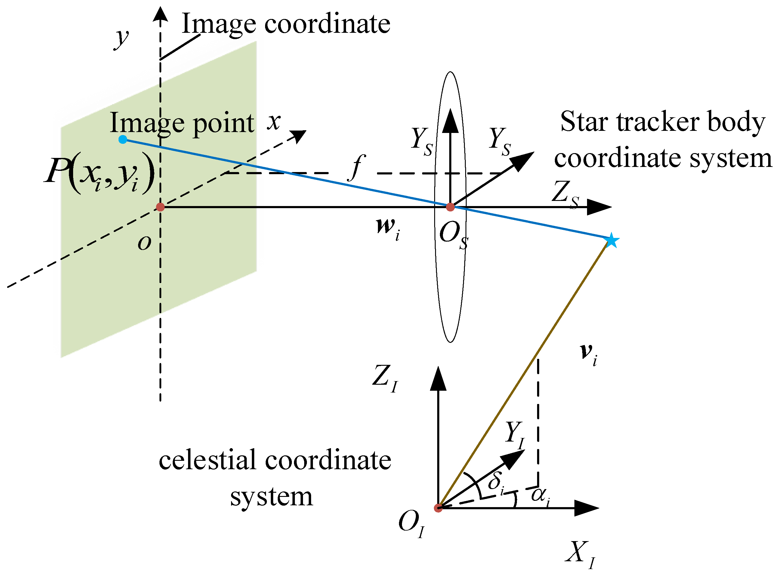
The star tracker is a high-accuracy vision device, which uses star positions to determine satellite attitude. Coordinate systems related to attitude measurement are shown in Figure 1, $o_I-x_I{y}_I{z}_I$ represents the celestial coordinate system. $o-xy$ represents the image plane coordinate system. $o_s-X_s{Y}_s{Z}_s$ represents the body coordinate system of the star tracker. The position vector of the navigation star $i$ in the celestial coordinate system is $v_i$, which is denoted as $\left({\alpha }_i,{\delta }_i\right)$, where ${\alpha }_i$ is ascension and ${\delta }_i$ is declination. The position vector of the navigation star $i$ in the body coordinate system of the star tracker is $w_i$ and the coordinates of the navigation star $i$ in the image plane coordinate system is denoted as $\left(x_i,y_i\right)$.

According to the transformation relationship between the spherical coordinate system and the rectangular coordinate system, the direction vector of the navigation star $i$ in the celestial coordinate system can be expressed as [24]:

$${\mathit{v}}_i=\left[\begin{array}{c}\cos {\alpha }_i\cos {\delta }_i\\ \sin {\alpha }_i\cos {\delta }_i\\ \sin {\delta }_i\end{array}\right]$$

(1)

According to the projection transformation relationship between the star tracker body coordinate system and the image plane coordinate system, the direction vector of the star $i$ in the body coordinate system of the star tracker can be expressed as [25]:

$${\mathit{w}}_i=\frac{1}{\sqrt{{\left(x_i-x_0\right)}^2+{\left(y_i-y_0\right)}^2+f^2}}\left[\begin{array}{l}-\left(x_i-x_0\right)\\ -\left(y_i-y_0\right)\\ f\end{array}\right]$$

(2)

where $f$ is the focal length of the star tracker, and $\left(x_0,y_0\right)$ is the coordinates of the principal point on the image plane. There is a coordinate transformation relationship between ${\mathit{w}}_i$ and ${\mathit{v}}_i$ [26]:

$${\mathit{w}}_i={\mathit{A}}_I^s{\mathit{v}}_i$$

(3)

where ${\mathit{A}}_I^s$ is the attitude transformation matrix from the celestial coordinate system $o_I-x_I{y}_I{z}_I$ to the body coordinate system of the star tracker $o_s-X_s{Y}_s{Z}_s$.

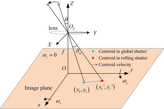
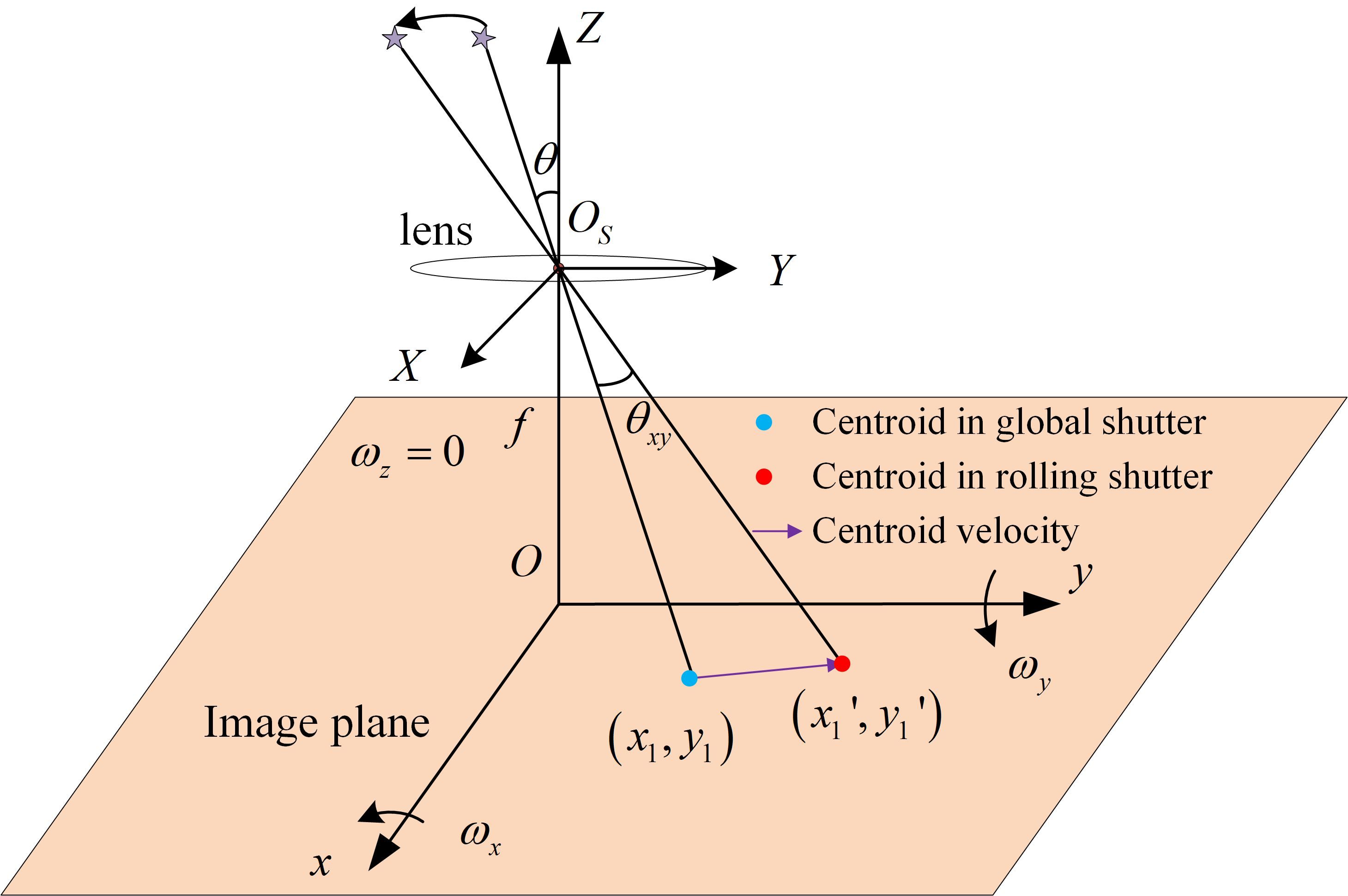
When the star tracker moves, the change of attitude makes the coordinates of the star in the imaging coordinate system change with time. The velocity of the star centroid on the image plane is determined by the angular velocity of the star tracker. The rotation model of the star tracker is shown in Figure 2, where ${\omega }_x$ is the angular velocity around the x-axis, ${\omega }_y$ is the angular velocity around the y-axis, ${\omega }_z$ is the angular velocity around the z-axis, $\left(x_0,y_0\right)$ is the centroid coordinate of star $i$ at the initial moment $t_0$, and $\left(x_1,y_1\right)$ is the centroid coordinate at the next moment $t_0+\Delta t$.

Suppose that the coordinate of the star position vector at the moment $t_0$ in the body coordinate system of the star tracker is ${\mathit{w}}_{i(t_0)}$ and the coordinate of the vector at moment $t_0+\Delta t$ in the body coordinate system of star tracker is ${\mathit{w}}_{i(t_0+\Delta t)}$, the transformation relationship between ${\mathit{w}}_{i(t_0)}$ and ${\mathit{w}}_{i(t_0+\Delta t)}$ can be expressed [27]:

$${\mathit{w}}_{i\left(t+\Delta t\right)}=C_{t_0}^{t_0+\Delta t}\times {\mathit{w}}_{t_0}$$

(4)

where $C_{t_0}^{t_0+\Delta t}$ is the transformation matrix from the body coordinate system of the star tracker at the moment $t_0$ and the body coordinate system of the star tracker at the moment $t_0+\Delta t$. Since the star direction vector does not change with time, $C_{t_0}^{t_0+\Delta t}$ can be obtained according to Equation (3):

$$C_t^{t+\Delta t}=A_{t+\Delta t}{A}_t^T$$

(5)

When $\Delta t$ is sufficiently small, $C_{t_0}^{t_0+\Delta t}$ can be represented as follows [28]:

$$C_t^{t+\Delta t}=\left[\begin{array}{ccc}1& {\omega }_z\Delta t& -{\omega }_y\Delta t\\ -{\omega }_z\Delta t& 1& {\omega }_x\Delta t\\ {\omega }_y\Delta t& -{\omega }_x\Delta t& 1\end{array}\right]$$

(6)

Substituting Equation (6) into Equation (4), the motion model of the star centroid can be simplified as follows:

$$\{\begin{array}{l}{x}_{i\left(t_1\right)}=x_{i\left(t_0\right)}+y_{i\left(t\right)}{\omega }_z\Delta t+f{\omega }_y\Delta t\\ y_{i\left(t_1\right)}=y_{i\left(t_0\right)}-x_{i\left(t\right)}{\omega }_z\Delta t-f{\omega }_x\Delta t\end{array}$$

(7)

According to Equation (7), when ${\omega }_z$ is not equal to zero, the star centroid velocity on the image plane changes nonlinearly. It is difficult to obtain the complete motion state of the star tracker directly from the image.

2.2. Installation Mode Design

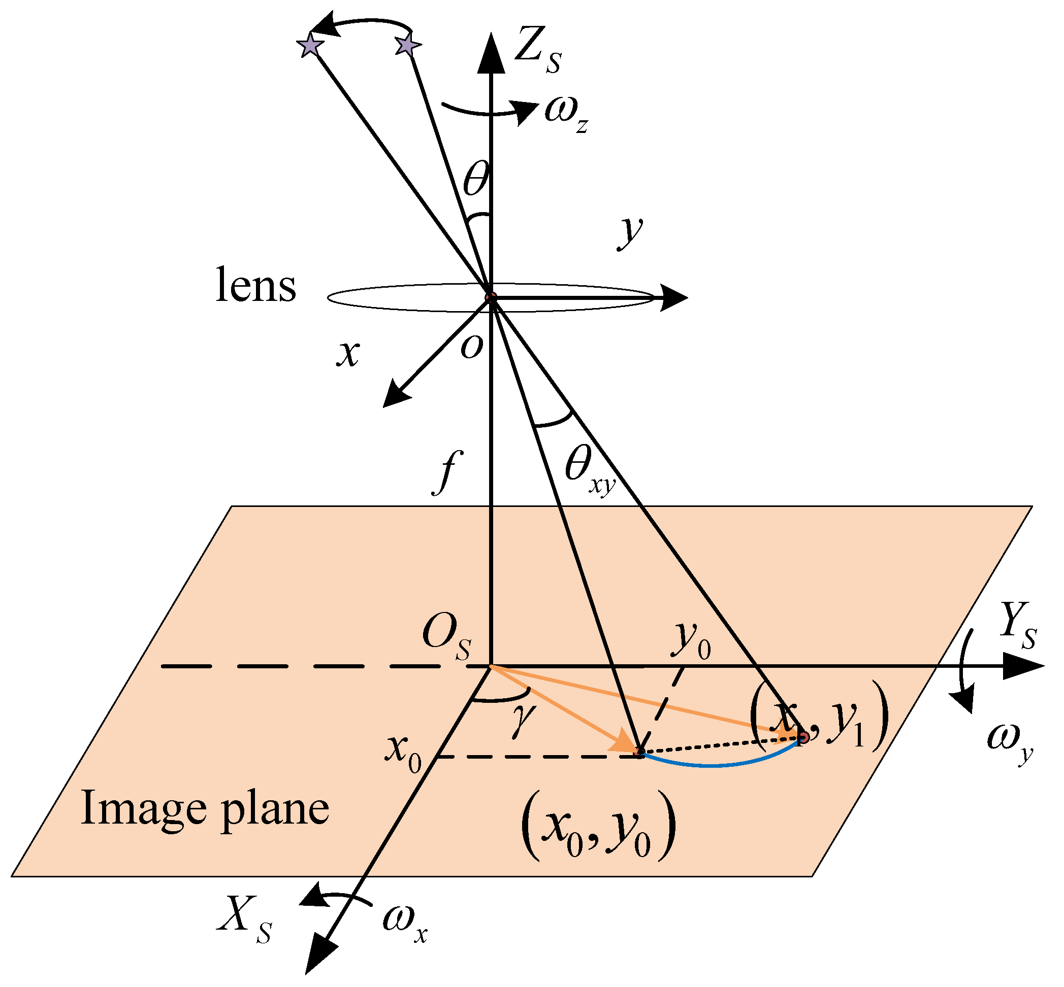
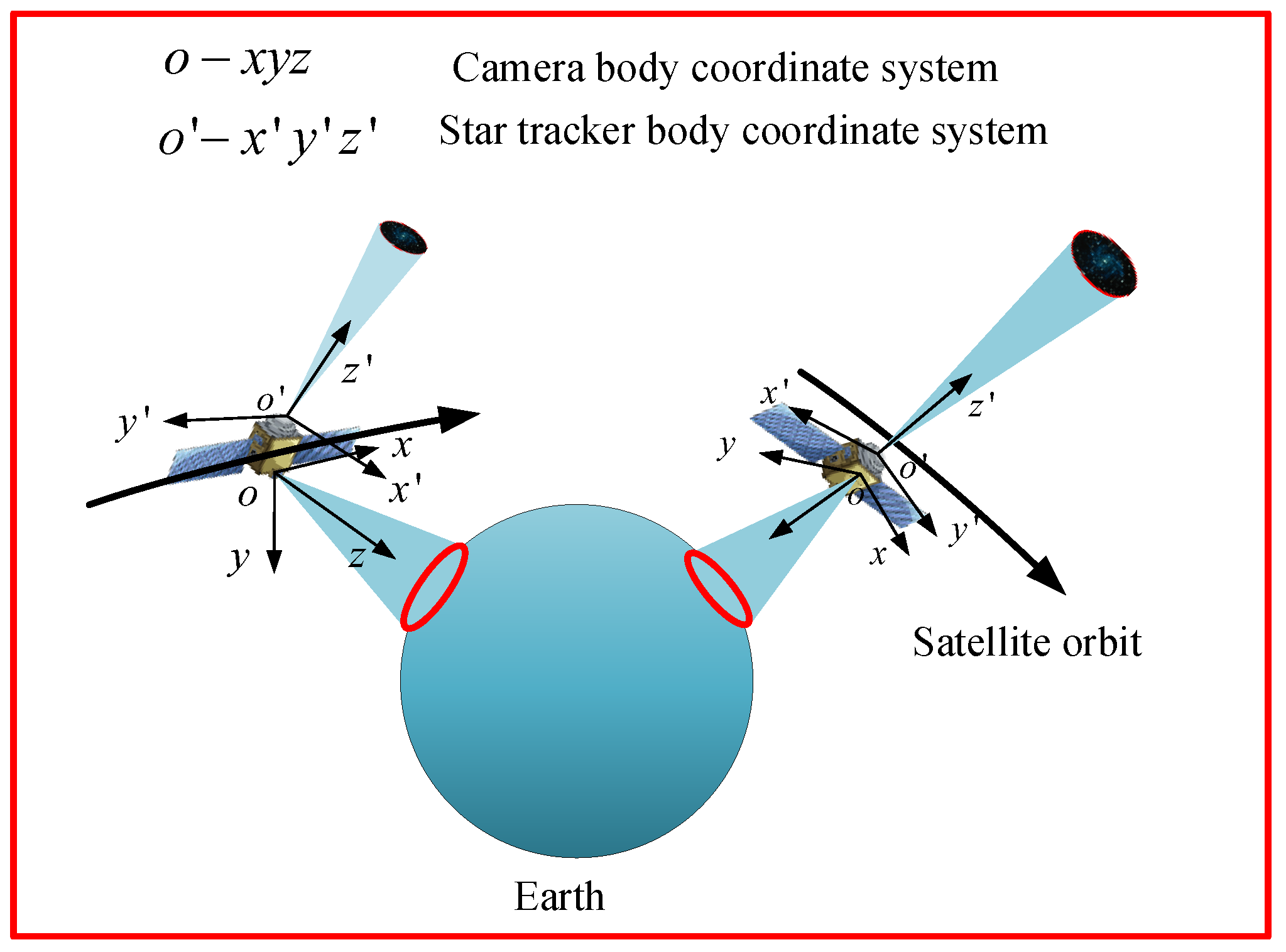
To simplify the relationship between the star centroid velocity and the star tracker angular velocity, the angular velocity around the optical axis of the star tracker ${\omega }_z$ should be zero according to the Equation (7). However, the star tracker angular velocity is due to the satellite angular velocity, which is normally planned according to the mission [29]. The relationship between the two angular velocities are related by the installation matrix [30]. The same satellite angular velocity will lead to different star tracker angular velocities with different installation directions. Therefore, the condition that ${\omega }_z$ is equal to zero can be achieved by changing the installation direction in a certain mission. In the field of remote sensing, most imaging tasks require the angular velocity of the optical axis of the space camera be kept at zero to ensure the high quality of the image [31,32,33]. Consequently, a specifical star tracker installation direction is proposed in this paper. As shown in Figure 3, the optical axis of the star tracker and the optical axis of the space camera are installed in the opposite direction. In this specific installation direction, ${\omega }_z$ is equal to zero when the satellite is imaging. This paper does not consider other cases where the ${\omega }_z$ is not zero.

Substituting ${\omega }_z$ equal to zero in Equation (7), the velocity of the star centroid on the image plane of the star tracker can be obtained as follows:

$$\left[\begin{array}{c}{v}_x\\ v_y\end{array}\right]=\left[\begin{array}{cc}0& f\\ -f& 0\end{array}\right]\left[\begin{array}{c}{\omega }_x\\ {\omega }_y\end{array}\right]$$

(8)

where $v_x$ and $v_y$ are the velocity of the star centroid in the x-direction and the y-direction, respectively.

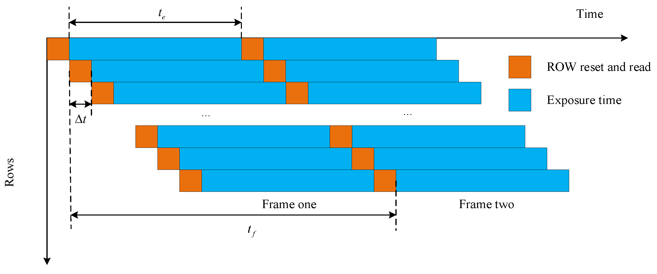
After determining the velocity of the satellite, the centroid distortion under rolling shutter exposure can be analyzed. Figure 4 shows the exposure process of the star tracker under rolling shutter exposure mode. Each row on the CMOS sensor starts to be exposed successively at a fixed interval. The exposure time of each row is the same, but the initial exposure time differs by a fixed value. The different rows in the image recorded information at different moments. The exposure time of each line is $t_e$, and there is a delay $\Delta t$ before the beginning of the exposure time between each row in rolling shutter exposure mode.

Compared to the global exposure mode, the error caused by the rolling shutter is shown as follows:

$$\{\begin{array}{l}\Delta x={\displaystyle {\int }_0^{t_d}f{\omega }_x\left(t\right)}dt\\ \Delta y={\displaystyle {\int }_0^{t_d}-f{\omega }_y}\left(t\right)dt\end{array}$$

(9)

where $\Delta x$ and $\Delta y$ are the centroid error in the $x$ direction and the $y$ direction, ${\omega }_x$ and ${\omega }_y$ is the angular velocity in the $x$ direction and the $y$ direction, $t_d$ is the duration between the reference time and the exposure time.

To further simplify Equation (9), the duration $t_d$ used in this paper is considered small enough to make the angular velocity remain constant. According to the research in [20], the relationship between $t_d$ and the reference moment can be expressed:

$$t_d=\frac{\Delta y}{\left(v_s-v_y\right)}$$

(10)

where $v_s$ is the scanning velocity of the image sensor, $v_y$ is the velocity of the star centroid in y-direction, and $\Delta y$ is the centroid error in the y-direction. In general, $v_y$ is much smaller than $v_s$. Thus, the exposure interval $t_0$ between two adjacent rows in rolling shutter imaging is constant. Substituting Equation (10) into Equation (9), the simplified expression of the centroid error can be obtained. However, due to the lack of the centroid error, the angular velocity of the star tracker still cannot be calculated directly.

2.3. Installation Mode Particle Swarm Optimization

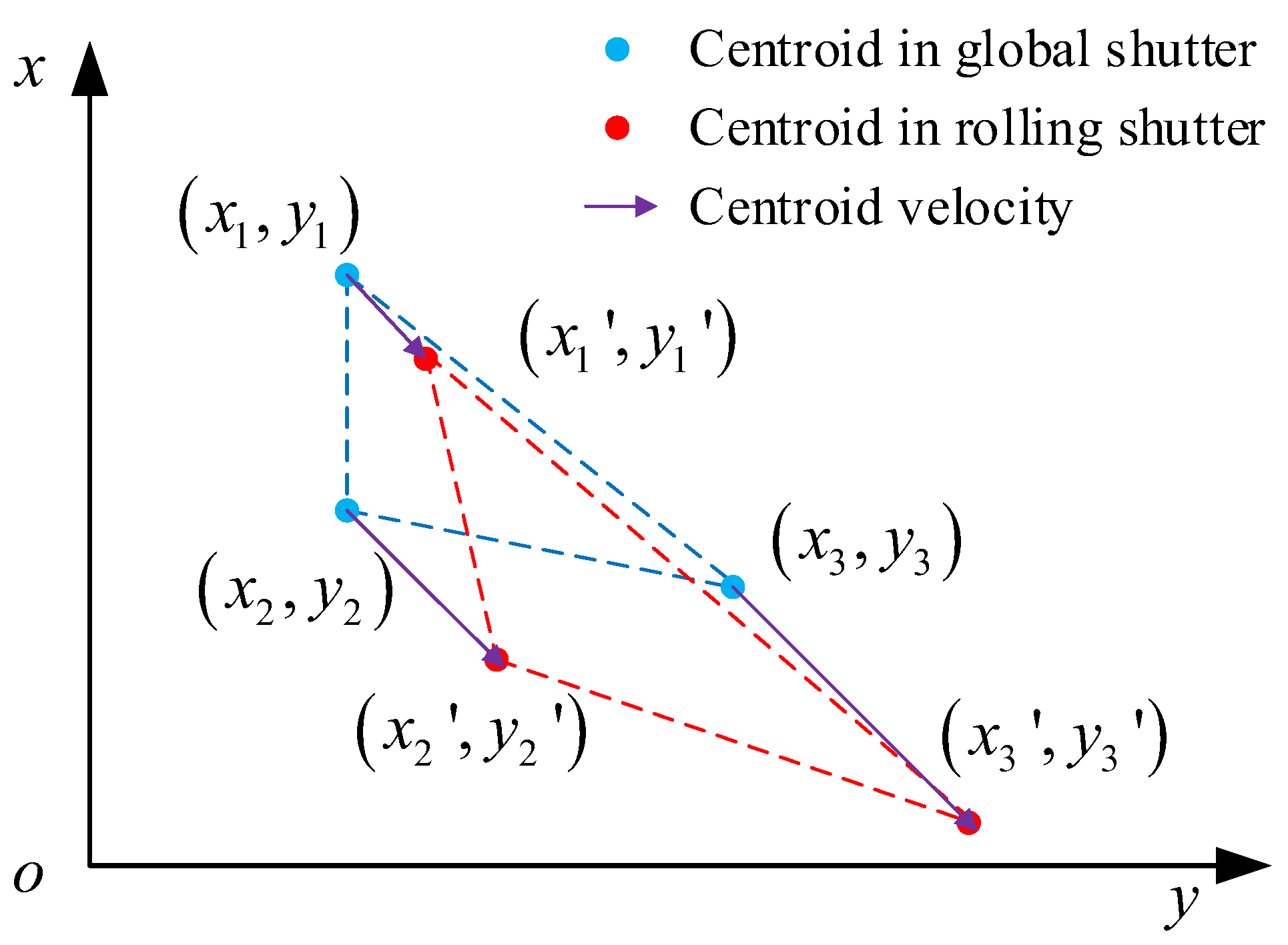
To calculate the angular velocity of the star tracker, the centroid error should be determined firstly. A method for calculating the centroid error based on the angular distance invariance and particle swarm optimization is introduced as follows. As shown in Figure 5, three adjacent star centroids are selected for calculation firstly. The $\left(x_i,y_i\right)$ denotes the centroid of star $i$ at the reference moment, $\left({x_i}^{\prime },{y_i}^{\prime }\right)$ denotes the star centroid of star $i$ at the image, and $\left(\Delta x_i,\Delta y_i\right)$ denotes the centroid error between the two star centroids, $i=1,2,3$.

The centroid error is caused by the motion of the star centroid from the beginning of the first line exposure to the end of the star exposure, which can be expressed:

$$\left[\begin{array}{l}\Delta x_i\\ \Delta y_i\end{array}\right]=\left[\begin{array}{cc}{y}_i{t}_0+T/2& 0\\ 0& y_i{t}_0+T/2\end{array}\right]\left[\begin{array}{c}{v}_x\\ v_y\end{array}\right]$$

(11)

where $v_x$ and $v_y$ are the velocity of star $i$ in the $x$ direction and the $y$ direction respectively, $t_0$ represents the exposure interval between lines of rolling shutter imaging, and $T$ is the exposure time. According to Equation (11), the velocity of the star can be solved after the centroid error $\left(\Delta x_i,\Delta y_i\right)$ and $y_i$ are determined.

To determine the velocity, a loss function with respect to $\left(\Delta x_1,\Delta y_1\right)$ is constructed as follows. According to Equation (11), the velocity of the star can be obtained:

$$\left[\begin{array}{c}{v}_x\\ v_y\end{array}\right]=\left[\begin{array}{cc}1/(y_1{t}_0+T/2)& 0\\ 0& 1/(y_1{t}_0+T/2)\end{array}\right]\left[\begin{array}{l}\Delta x_1\\ \Delta y_1\end{array}\right]$$

(12)

When the star tracker installation is the collinear reverse installation method, the velocity of the star centroid on the plane is constant according to Equation (8). Substituting Equation (12) into Equation (11), the star centroid error can be expressed:

$$\left[\begin{array}{c}\Delta x_i\\ \Delta y_i\end{array}\right]=\left[\begin{array}{cc}(y_i{t}_0+T/2)/(y_1{t}_0+T/2)& 0\\ 0& (y_i{t}_0+T/2)/(y_1{t}_0+T/2)\end{array}\right]\left[\begin{array}{l}\Delta x_1\\ \Delta y_1\end{array}\right]$$

(13)

According to the relationship between $\left(x_i,y_i\right)$ and $\left({x_i}^{\prime },{y_i}^{\prime }\right)$, $\left(x_i,y_i\right)$ can be expressed:

$$\left[\begin{array}{c}{x}_i\\ y_i\end{array}\right]=\left[\begin{array}{c}{x_i}^{\prime }\\ {y_i}^{\prime }\end{array}\right]-\left[\begin{array}{c}\Delta x_i\\ \Delta y_i\end{array}\right]$$

(14)

Substituting Equation (13) into Equation (14), the centroid of star $i$ at the reference moment can be expressed by $\left(\Delta x_1,\Delta y_1\right)$. After the derivation of the centroid of star $i$ at the reference moment is completed, the loss function is constructed as follow.

At the reference moment, the direction vector of the star $i$ in $o_s-X_s{Y}_s{Z}_s$ can be obtained by Equation (2) after the star centroid is determined by Equation (13). The angular distance between star $i$ and star $j$ in the body coordinate system of the star tracker is defined as:

$${\theta }_{ij}=\arccos \frac{{\mathit{w}}_i\cdot {\mathit{w}}_j}{\left|{\mathit{w}}_i\right|\cdot \left|{\mathit{w}}_j\right|}$$

(15)

According to the angular distance invariance, the angular distance between two stars is constant. The angle distance between the identified stars can be obtained from the star catalog. Considering the actual engineering application conditions, this paper assumes that the stars in images have already been identified. Therefore, the loss function is designed based on the angular distance difference. According to Equations (13) and (14), if $\Delta x_1$ and $\Delta y_1$ can be determined, all of the star centroids in the image can be obtained. Thus, $\Delta x_1$ and $\Delta y_1$ are selected to the dependent variable of the loss function. The loss function is defined as:

$$J\left(\Delta x_1,\Delta y_1\right)={\displaystyle \sum {\Vert {\theta }_{ij}-{{\theta }_{ij}}^{\prime }\Vert }_2}$$

(16)

where ${\theta }_{ij}$ is the angular distance between star $i$ and star $j$ obtained from star catalog, and ${{\theta }_{ij}}^{\prime }$ is angular distance calculated by using $\Delta x_1$ and $\Delta y_1$. To minimize this loss function, this paper uses the particle swarm optimization algorithm.

The particle swarm optimization algorithm is a population-based random search method, which uses the foraging behavior of birds. The particle swarm optimization algorithm uses a certain number of particles that represents the potential solution and changes the position of these particles by the equations listed below:

$$\begin{array}{l}{V}_{n+1}^i=w{V}_n^i+c_1{r}_1\left(P_n^i-X_n^i\right)+c_2{r}_2\left(G_n^i-X_n^i\right)\\ X_{n+1}^i=X_n^i+V_{n+1}^i\end{array}$$

(17)

where $V_n^i$ represents the speed of the $i$th particle in $n$ generation, $X_n^i$ represents the position of the $i$th particle in $n$ generation, $P_n^i$ represents the previous best position of the $i$th particle in $n$ generation, $G_n^i$ represents the best position of all the particles in $n$ generation, $w$ represents the inertia weight, $c_1$ and $c_2$ are acceleration constants, and $r_1$ and $r_2$ represents a random number uniformly distributed in the range $\left[0,1\right]$. According to [34], the inertia weight $w$ is set as:

$$w_g=w_{\min }+\frac{N-g}{N}\left(w_{\max }-w_{\min }\right)$$

(18)

where $w_g$ is the inertia weight in Nth generation, $N$ is the total number of generation, $w_{\max }$ is equal to 0.9, and $w_{\min }$ is equal to 0.4. The acceleration constants $c_1$ and $c_2$ are set to integer 2. The Algorithm 1 proposed in this paper is shown as follow:

Algorithm 1 Standard PSO pseudocode

1: Algorithm input: particle number $N_0$, the maximum number of iterations N, inertia angular velocity ${\omega }_0$

2: Algorithm output: optimal angular velocity $G_0$, the loss function $J$

3: Randomly generate velocity solutions

4: g = 0

5: while g < N do

6:                 for i = 1 to $N_0$ do

7:                         $V_{n+1}^i=w{V}_n^i+c_1{r}_1\left(P_n^i-X_n^i\right)+c_2{r}_2\left(G_n^i-X_n^i\right)$

8:                         $X_{n+1}^i=X_n^i+V_{n+1}^i$

9:                 end for

10:               computer fitness function value $J(X_{n+1})$

11:               $P_{i,n+1}=\{\begin{array}{l}\begin{array}{cc}{P}_{i,n}& f\left(P_{i,n}\right)<f\left(X_{i,n+1}\right)\end{array}\\ \begin{array}{cc}{X}_{i,n+1}& f\left(P_{i,n}\right)\ge f\left(X_{i,n+1}\right)\end{array}\end{array}$

12:               Find the best solution $G_0$ in all the particles in the iteration

13:               if $f\left(G_0\right)<f\left(G_n\right)$

14:                         $G_{n+1}=G_0$

15:               else

16:                         $G_{n+1}=G_n$

17:               n = n + 1

18: end

3. Results

In the previous sections, we analyzed the star centroid velocity model of the star tracker in the collinear installation, derived the star centroid error in the rolling shutter espouse mode, and proposed an angular velocity estimation algorithm based on particle swarm optimization to complete the error compensation. In this section, numerical simulations and field experiments are employed to verify the proposed method.

3.1. Simulation of Star Centroid Velocity with Collinear Installation

To simplify the relationship between the star centroid velocity and the angular velocity of a star tracker, a collinear reverse installation method is proposed in Section 2.2. However, there will be a control error between the actual angular velocity and the set value. The control error will cause the angular velocity around the optical axis of the star tracker ${\omega }_z$ is not equal to zero. This paper simulates the effect caused by the small value of ${\omega }_z$. The parameters used in the simulation are shown in the

Table 1. Parameters used in simulation.

Parameter	Value
Focal length	42 mm
Field of view	$18°\times 18°$
Resolution	$2048\times 1280$
Pixel length	5.5 μm
Exposure time	100 ms
Star magnitude limit	5.2 Mv

.

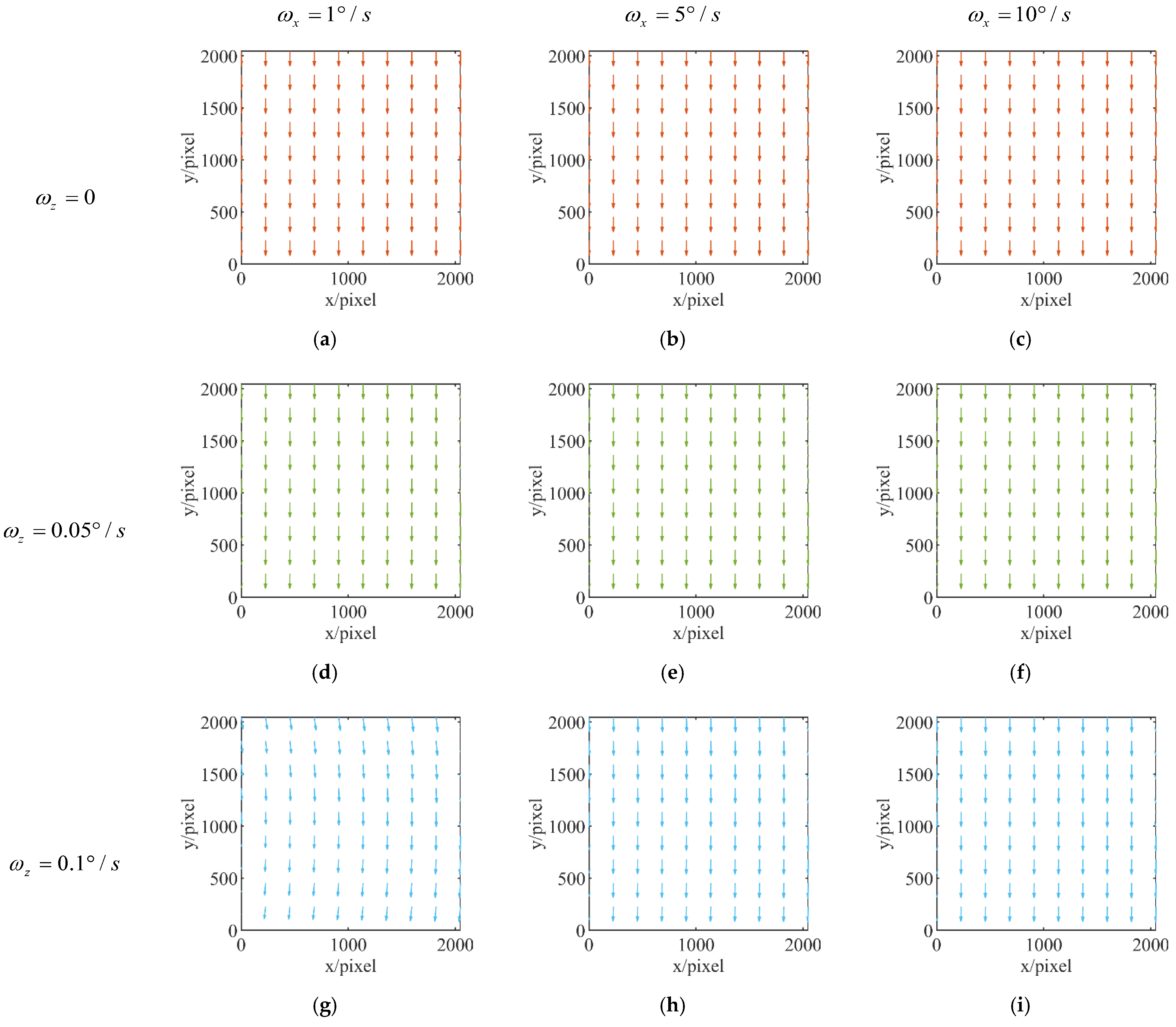
In the simulation, the angular velocity around the x axis of the star tracker ${\omega }_x$ is set to 1°/s, 5°/s, and 10°/s respectively and the angular velocity around the z axis of the star tracker ${\omega }_z$ is set to 0, 0.05°/s, and 0.1°/s. As shown in Figure 6, the velocity of the star centroid is simulated.

As shown in Figure 6, the direction of star centroid velocity remains straight when ${\omega }_z$ is equal to zero, and there is little effect on the velocity direction when ${\omega }_z$ is not equal to zero. To analyze the specific effect of ${\omega }_z$ on star centroid velocity, we analyze the magnitude and direction of the velocity when ${\omega }_z$ is equal to 1°/s. As shown in Figure 7a, the direction of the velocity caused by ${\omega }_z$ is symmetrical about the center of the field of view, and the velocity vector at the edge of the field of view has a larger magnitude than the velocity vector at the center of the field of view. The maximum velocity does not exceed 1.5 pixel/s. The star centroid is determined by the velocity and exposure time. The angular velocity error caused by the satellite control system is less than 0.01°/s [35]. Without considering the installation direction error, the angular velocity component in the z-direction is smaller than 0.01°/s during the imaging process, and the exposure time of the star tracker is no more than 200 ms. The influence of the velocity component in the z-direction is considered small enough to be ignored in this paper.

3.2. Simulation Experiment

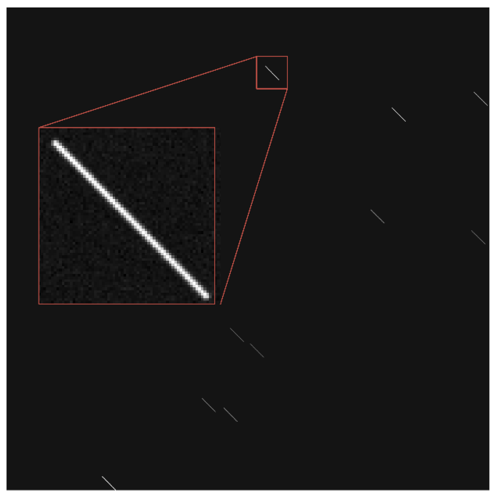
To verify the effectiveness of the proposed algorithm, a simulation experiment was carried out. The star tracker parameters used in the simulation are shown in Table 1. Before completing the simulation, the star images obtained in the rolling shutter exposure mode are synthesized firstly. A discussion of star images in the rolling shutter exposure mode can be found in [36]. Random Gaussian noise with a mean value of 0.25 and a variance of 0.001 was added to the background noise of the synthesized star images. A synthesized star image is shown in Figure 8.

Star images are synthesized at angular velocities of 0.5°/s, 1°/s, 1.5°/s, 2°/s, 2.5°/s, 3°/s, and 5°/s, respectively. The centroid extraction and star identification are carried out and the theoretical angular distance value is obtained from the star catalog after star identification. Then, the proposed algorithm is tested by the image captured in the field experiment.

3.2.1. Convergence Simulation

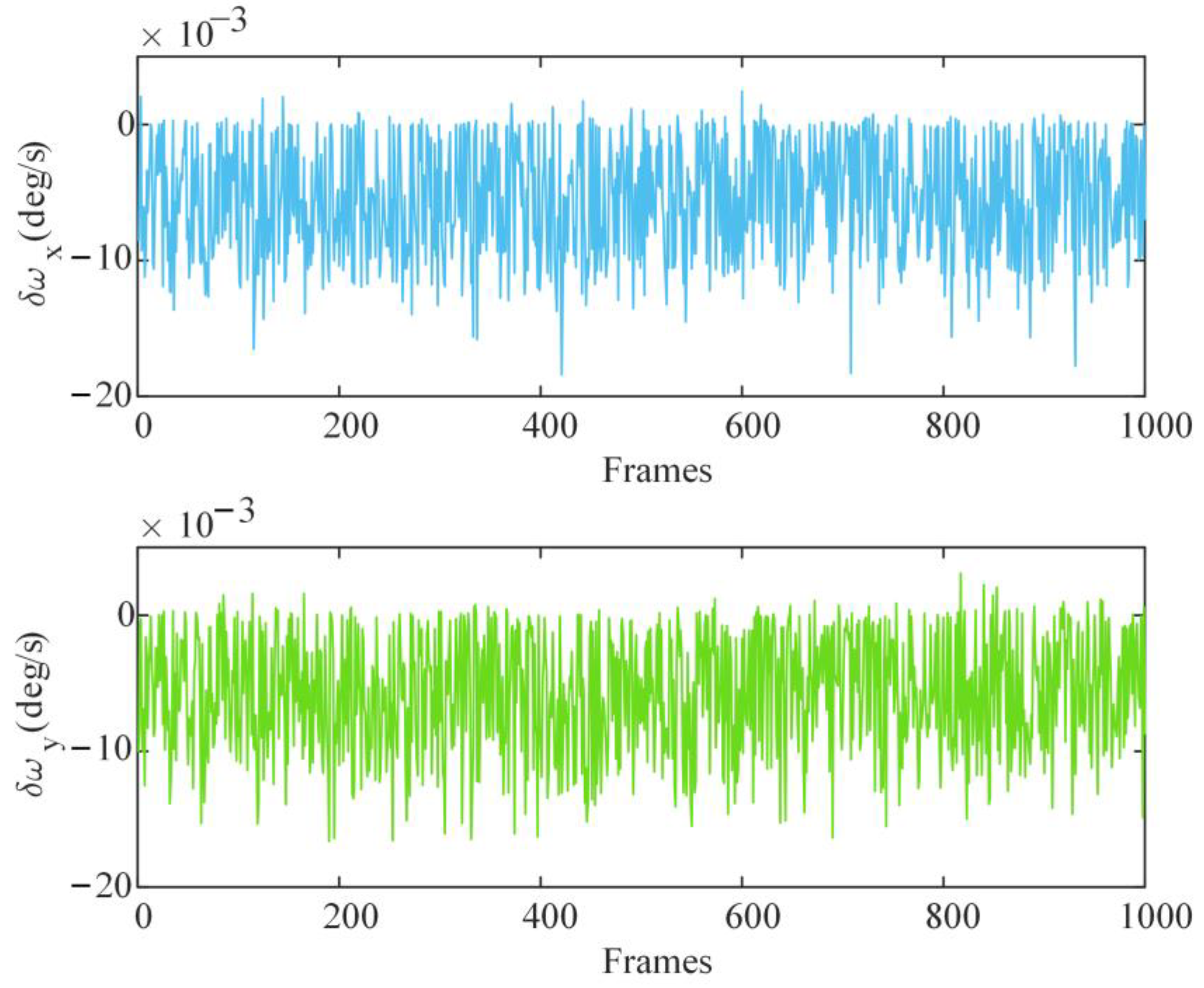
The images that are synthesized when ${\omega }_x$ and ${\omega }_y$ are set to 1°/s are used to test the convergence of the algorithm. The results of the angular velocity error obtained by the algorithm is shown in Figure 9. The velocity error is no more than 0.002°/s.

The convergence times of generations in the above experiment are counted as shown in Figure 10. Most of the convergence times are less than 10, which will not cause excessive time consumption.

3.2.2. Robustness of the Algorithm under Different Angular Velocities and Different Position Noise

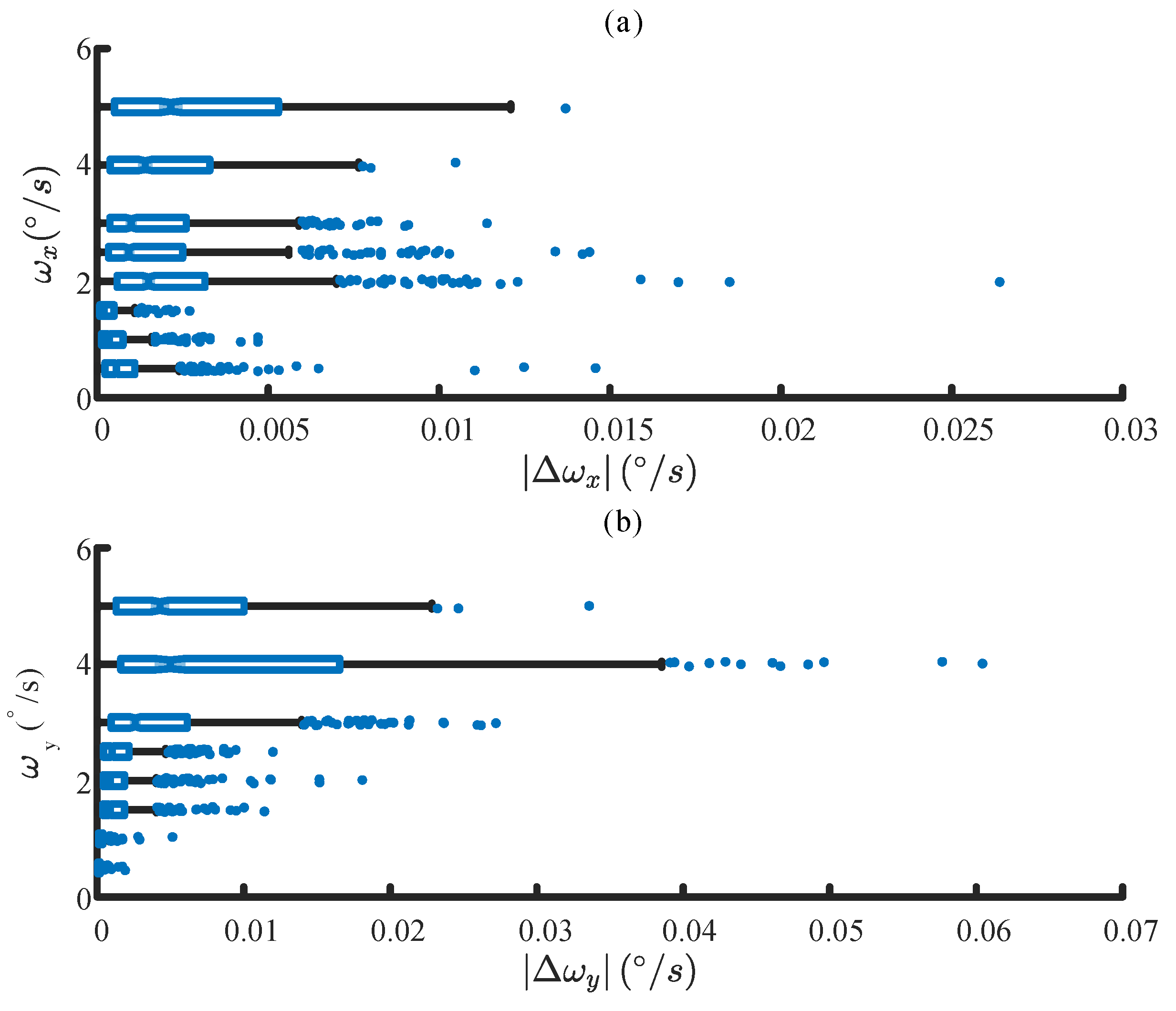
To test the robustness of the algorithm under different angular velocities, the star images synthesized under different angular velocities are tested. The number of experiments per angular velocity is set to 500. A box chart of the absolute value of the angular velocity estimation error is shown in Figure 11. As the angular velocity increases, the absolute value of the velocity error increases, and the number of outliers decreases. Comparing the accuracy of the estimated angular velocity in two directions, the accuracy of velocity in the x-direction is greater than that in the y-direction. All the maximum values of the absolute velocity error in both directions are less than 0.1°/s, which maintains a high accuracy of angular velocity estimation.

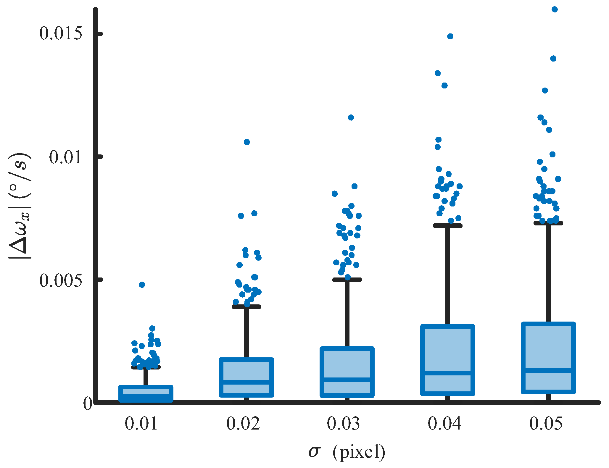
In the actual measurement environment, the performance of a star tracker will be affected by detector noise. To test the robustness of the algorithm under different noise conditions, star images synthesized under different position noise were tested. The star images used in the noise test were synthesized when ${\omega }_x$ were equal to 3°/s and when ${\omega }_y$ was zero. Gaussian position noise was added during the synthesis of the star maps. The Gaussian noise was added to the star centroid in the process of star image generation. The mean of the noise was set to zero, and the variance $\sigma$ was set from 0.01 pixels to 0.05 pixels. The number of experiments per variance is set to 500. The box chart of the absolute value of the angular velocity estimation error is shown in Figure 12. As the variance of position noise increases, the accuracy of angular velocity estimation decreases. The maximum value of outliers is also positively correlated with noise variance. When the position noise variance is less than 0.05 pixels, the fourth quartile of velocity estimation error is smaller than 0.01°/s.

3.3. Field Experiment

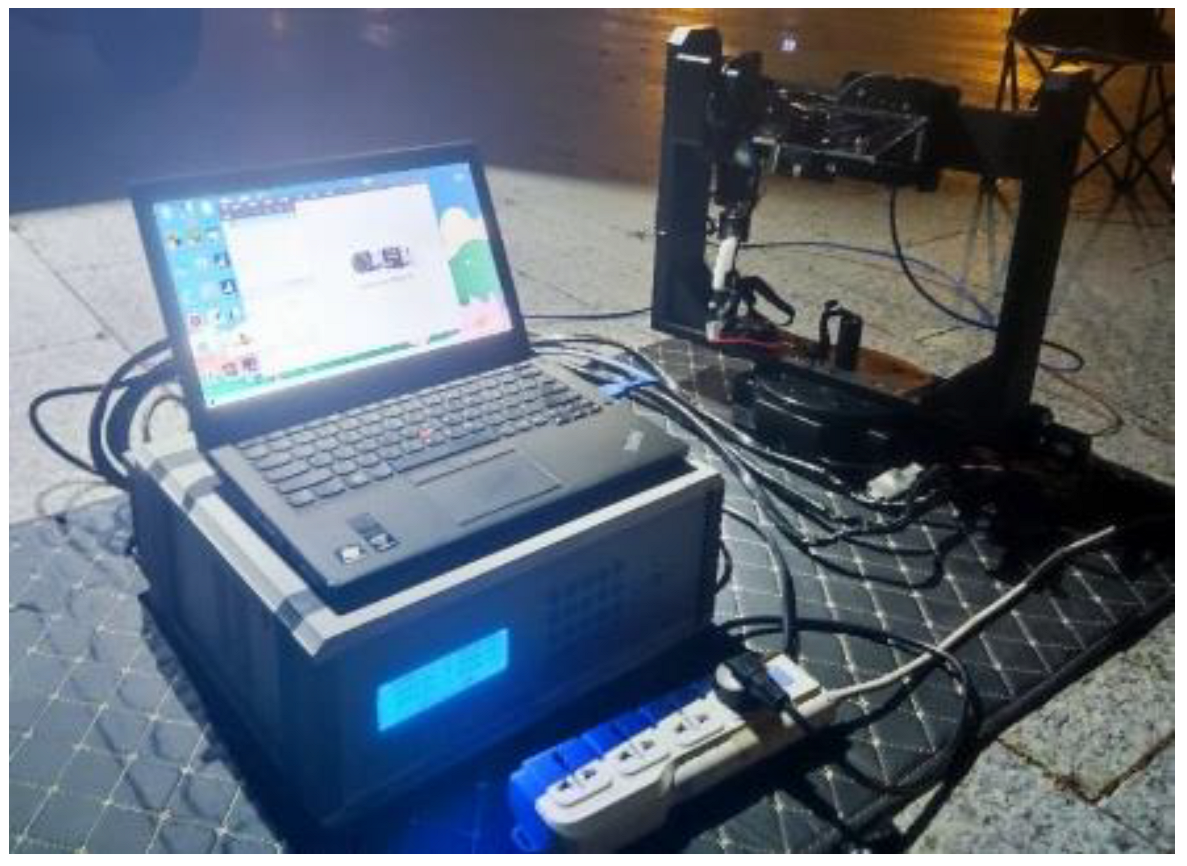
To verify the effectiveness of the proposed algorithm, a field experiment was carried out, and the experimental system is shown in Figure 13, which consists of a turntable and a rolling shutter camera whose parameters is shown in Table 1. A total of 500 frames of star images were collected at the angular velocity of 0.5°/s, 1°/s, 3°/s, and 5°/s respectively. The centroid extraction and star identification were carried out after image preprocessing, and the theoretical angular distance value was obtained from the star catalog after star identification. Then, the proposed algorithm was tested by the image captured in the field experiment.

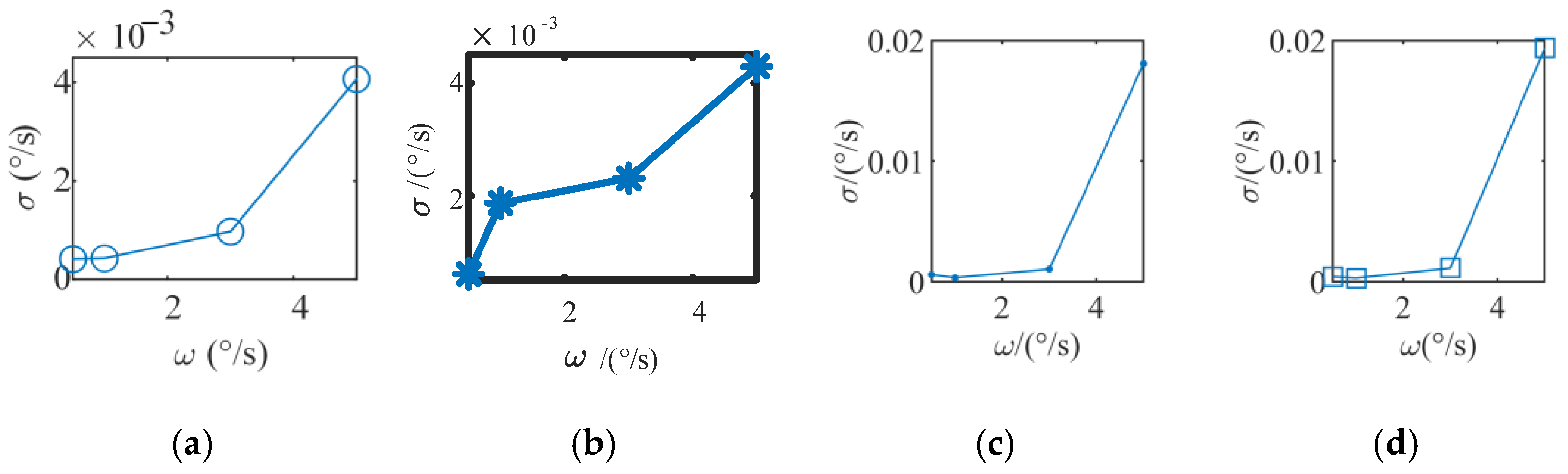
To test the robustness of the algorithm under different angular velocities, the star images taken under angular velocities are tested. There are three different kinds of images captured in field experiments. The first kind of image is obtained when only ${\omega }_x$ exists. The second one is obtained when only ${\omega }_y$ exists. The last one is obtained when ${\omega }_x$ is equal to ${\omega }_y$. To quantify the calculation results, the root mean square error (RMSE) of the angular velocity is calculated by:

$$\sigma =\sqrt{\frac{{\displaystyle \sum _{i=1}^n{\left({\omega }^{\prime }-\omega \right)}^2}}{n}}$$

(19)

The RMSE of the angular velocity error is shown in Figure 14. When the angular velocity is less than 5°/s, the maximum RMSE does not exceed 0.02°/s.

4. Discussion

In this paper, the accuracy of the proposed algorithm was tested by simulation and experiment. In this paper, some factors are ignored, which objectively exist in practical application. In Section 3.1, the centroid error caused by control error is simulated. Due to the existence of control error, ${\omega }_z$ will not be zero when the satellite is working. However, according to Equation (7), the centroid velocity component due to ${\omega }_z$ is proportional to the position of the star centroid in the image plane. The length of the image sensor is far less than the focal length of the star tracker, which makes the star centroid velocity caused by the control error small enough to be ignored. However, the angular velocity in the z-direction caused by the installation direction error can produce considerable centroid error, which means that the premise of the proposed algorithm is high installation accuracy.

In Section 3.2, the accuracy of the algorithm is analyzed. As shown in Figure 11, the accuracy of ${\omega }_x$ will be slightly higher than that of ${\omega }_y$. This is because $\Delta y$ is more constrained than $\Delta x$, which is directly related to ${\omega }_x$. The accuracy of angular velocity estimation is related to the accuracy of dynamic star map extraction. The extraction of a dynamic star map is a comprehensive and complex problem. In this paper, centroid position noise is used to represent the errors introduced in dynamic star map extraction. The robustness of the algorithm to position noise is tested in the simulation experiment. Figure 12 shows the good robustness of the position noise of the proposed algorithm. It is worth mentioning that the method proposed in this paper only needs three adjacent star coordinates, which is ideal for high-frequency attitude measurement. At the same time, the small number of stars used means that the accuracy of velocity estimation is highly dependent on the accuracy of star extraction. How to obtain high precision centroid results by star point trailing will be studied later.

5. Conclusions

In this paper, a method of angular velocity estimation using the particle swarm optimization algorithm for a high-dynamic star tracker in rolling shutter exposure. According to the feature that the optical axis does not rotate during satellite imaging, a collinear installation method for star trackers is proposed to simplify the velocity variation of star centroid motion. Then, a loss function is proposed based on angular distance invariance, and the particle swarm optimization algorithm is adopted to solve the loss function. Experimental results show that the proposed algorithm can converge quickly within 50 times and that the RMSE of angular velocity is better than 0.02°/s and under the angular velocity is no more than 5°/s. The results present in this article lay a foundation for further improving the measurement accuracy and frequency of star trackers. In this paper, it is assumed that the satellite does not rotate around the optical axis of the camera, which is applicable to most application scenarios. The assumption limits the application scenarios of the algorithm. How to improve the application scope of the algorithm will be the next research focus.

References

- Wang, J.D.; Du, L.; Li, Y.C.; Lyu, G.X.; Chen, B. Attitude and Size Estimation of Satellite Targets Based on ISAR Image Interpretation. IEEE Trans. Geosci. Remote Sens. 2022, 60, 5109015. [Google Scholar] [CrossRef]
- Fan, Q.Y.; Chen, C.Y.; Wang, G.Y.; Wei, X.G. Parameters Estimation of Nutational Satellite Based on Sun Sensor. IEEE Trans. Instrum. Meas. 2022, 71, 7000508. [Google Scholar] [CrossRef]
- Kouyama, T.; Kanemura, A.; Kato, S.; Imamoglu, N.; Fukuhara, T.; Nakamura, R. Satellite Attitude Determination and Map Projection Based on Robust Image Matching. Remote Sens. 2017, 9, 90. [Google Scholar] [CrossRef] [Green Version]
- Yan, G.M.; Chen, R.T.; Weng, J. A super-fast optimal attitude matrix in attitude determination. Meas. Sci. Technol. 2021, 32, 095012. [Google Scholar] [CrossRef]
- Ding, J.; Dai, D.; Tan, W.; Wang, X.; Qin, S. Implementation of a real-time star centroid extraction algorithm with high speed and superior denoising ability. Appl. Opt. 2022, 61, 3115–3122. [Google Scholar] [CrossRef] [PubMed]
- Ni, Y.M.; Wang, X.S.; Dai, D.K.; Tan, W.F.; Qin, S.Q. Adaptive section non-uniformity correction method of short-wave infrared star images for a star tracker. Appl. Opt. 2022, 61, 6992–6999. [Google Scholar] [CrossRef]
- Wang, Y.L.; Wang, M.; Zhu, Y.; Long, X.X. Low frequency error analysis and calibration for multiple star sensors system of GaoFen7 satellite. Geo-Spat. Inf. Sci. 2022. [Google Scholar] [CrossRef]
- McKee, P.; Nguyen, H.; Kudenov, M.W.; Christian, J.A. StarNAV with a wide field-of-view optical sensor. Acta Astronaut. 2022, 197, 220–234. [Google Scholar] [CrossRef]
- Hancock, B.R.; Stirbl, R.C.; Cunningham, T.J.; Pain, B.; Wrigley, C.J.; Ringold, P.G. CMOS active pixel sensor specific performance effects on star tracker/imager position accuracy. In Proceedings of the Conference on Functional Integration of Opto-Electro-Mechanical Devices and Systems, San Jose, CA, USA, 24–25 January 2001; pp. 43–53. [Google Scholar]
- Liang, C.K.; Chang, L.W.; Chen, H.H. Analysis and compensation of rolling shutter effect. IEEE Trans. Image Process. 2008, 17, 1323–1330. [Google Scholar] [CrossRef] [Green Version]
- He, Z.-Y.; Wei, P. New method for 2D velocity measurement based on electronic rolling shutter. In Proceedings of the International Conference on Photoelectronic Detection and Imaging, Beijing, China, 9–12 September 2007. [Google Scholar]
- Rengarajan, V.; Balaji, Y.; Rajagopalan, A.N.; Ieee. Unrolling the Shutter: CNN to Correct Motion Distortions. In Proceedings of the 30th IEEE/CVF Conference on Computer Vision and Pattern Recognition (CVPR), Honolulu, HI, USA, 21–26 July 2017; pp. 2345–2353.
- Wei, M.S.; Xing, F.; You, Z. An implementation method based on ERS imaging mode for sun sensor with 1 kHz update rate and 1″ precision level. Opt. Express 2013, 21, 32524–32533. [Google Scholar] [CrossRef]
- Zhang, B.-Y.; Kong, D.-Z.; Liu, J.-G.; Wu, X.-X.; Dong, D.-Y. Compensation of star image motion for a CMOS image sensor with a rolling shutter. Chin. Opt. 2020, 13, 1276–1284. [Google Scholar] [CrossRef]
- Enright, J.; Dzamba, T. Rolling Shutter Compensation for Star Trackers. In Proceedings of the AIAA Guidance, Navigation, and Control Conference, Minneapolis, MN, USA, 13–16 August 2012. [Google Scholar]
- He, L.; Zhao, R.; Ma, Y.; Hou, Y.; Zhu, Z.; Zeng, S. Navigation Stars Correction Method of Rolling Shutter Exposure Star Tracker Based on Time Domain Constraint. Acta Photonica Sin. 2021, 50, 128. [Google Scholar] [CrossRef]
- He, L.; Ma, Y.; Zhao, R.; Hou, Y.; Zhu, Z. High Update Rate Attitude Measurement Method of Star Sensors Based on Star Point Correction of Rolling Shutter Exposure. Sensors 2021, 21, 5724. [Google Scholar] [CrossRef] [PubMed]
- Yoon, H. Single-Frame Rolling Shutter Corrector for Star Trackers. J. Spacecr. Rocket. 2019, 56, 292–297. [Google Scholar] [CrossRef]
- Schiattarella, V.; Spiller, D.; Curti, F. Star identification robust to angular rates and false objects with rolling shutter compensation. Acta Astronaut. 2020, 166, 243–259. [Google Scholar] [CrossRef]
- Li, Y.; Wei, X.; Li, J.; Wang, G. Error Correction of Rolling Shutter Effect for Star Sensor Based on Angular Distance Invariance Using Single Frame Star Image. IEEE Trans. Instrum. Meas. 2022, 71, 7003213. [Google Scholar] [CrossRef]
- Boussaid, I.; Lepagnot, J.; Siarry, P. A survey on optimization metaheuristics. Inf. Sci. 2013, 237, 82–117. [Google Scholar] [CrossRef]
- Dokeroglu, T.; Sevinc, E.; Kucukyilmaz, T.; Cosar, A. A survey on new generation metaheuristic algorithms. Comput. Ind. Eng. 2019, 137, 106040. [Google Scholar] [CrossRef]
- Hussain, K.; Salleh, M.N.M.; Cheng, S.; Shi, Y.H. Metaheuristic research: A comprehensive survey. Artif. Intell. Rev. 2019, 52, 2191–2233. [Google Scholar] [CrossRef] [Green Version]
- Zhao, S.; Wang, X.; Tan, W.; Dai, D.; Qin, S. Error coupling analysis of the laboratory calibration method for a star tracker. Appl. Opt. 2021, 60, 2372–2379. [Google Scholar] [CrossRef]
- Zhang, C.F.; Niu, Y.X.; Zhang, H.; Lu, J.Z. Optimized star sensors laboratory calibration method using a regularization neural network. Appl. Opt. 2018, 57, 1067–1074. [Google Scholar] [CrossRef] [PubMed]
- Zhang, H.; Niu, Y.; Lu, J.; Zhang, C.; Yang, Y. On-orbit calibration for star sensors without priori information. Opt. Express 2017, 25, 18393–18409. [Google Scholar] [CrossRef] [PubMed]
- Han, J.; Yang, X.; Xu, T.; Fu, Z.; Chang, L.; Yang, C.; Jin, G. An End-to-End Identification Algorithm for Smearing Star Image. Remote Sens. 2021, 13, 4541. [Google Scholar] [CrossRef]
- Song, J.N.; Zhang, Z.X.; Iwasaki, A.; Wang, J.H.; Sun, J.; Sun, Y. An Augmented H-infinity Filter for Satellite Jitter Estimation Based on ASTER/SWIR and Blurred Star Images. IEEE Trans. Aerosp. Electron. Syst. 2021, 57, 2637–2646. [Google Scholar] [CrossRef]
- Wang, F.; Xi, R.; Yue, C.; Li, H.; Cao, X. Conceptual rotational mode design for optical conical scanning imaging small satellites. Sci. China Technol. Sci. 2020, 63, 1383–1395. [Google Scholar] [CrossRef]
- Fang, J.C.; Ning, X.L. Installation Direction Analysis of Star Sensors by Hybrid Condition Number. IEEE Trans. Instrum. Meas. 2009, 58, 3576–3582. [Google Scholar] [CrossRef]
- Han, J.L.; Yang, X.B.; Yue, W.; Xu, T.T.; Wang, S.E.; Chang, L.; Yang, C.L. Image Motion of Remote Sensing Camera with Wide Field of View Over the Antarctic and Arctic. IEEE J. Sel. Top. Appl. Earth Obs. Remote Sens. 2021, 14, 3475–3484. [Google Scholar] [CrossRef]
- Xu, T.; Yang, X.; Wang, S.; Han, J.; Chang, L.; Yue, W. Imaging Velocity Fields Analysis of Space Camera for Dynamic Circular Scanning. IEEE Access 2020, 8, 191574–191585. [Google Scholar] [CrossRef]
- Jiang, L.; Yang, X. Study on Enlarging the Searching Scope of Staring Area and Tracking Imaging of Dynamic Targets by Optical Satellites. IEEE Sens. J. 2021, 21, 5349–5358. [Google Scholar] [CrossRef]
- Li, D.; Xu, J.; Zhu, B.; He, H. A calibration method of DVL in integrated navigation system based on particle swarm optimization. Measurement 2022, 187, 110325. [Google Scholar] [CrossRef]
- Majumder, C.G.; Siva, M.S.; Kumar, A.; Philip, N.K.; Ieee. Control Algorithms for Improved High Pointing accuracy and Rate Stability in Agile Imaging Spacecrafts. In Proceedings of the 3rd Indian Control Conference (ICC), Indian Inst Technol Guwahati Campus, Guwahati, India, 4–6 January 2017; pp. 93–98. [Google Scholar]
- Li, Y.; Wei, X.; Li, J.; Wang, G. Imaging modeling and error analysis of the star sensor under rolling shutter exposure mode. Opt. Express 2021, 29, 15478–15496. [Google Scholar] [CrossRef] [PubMed]
Figure 1.
Coordinate system in attitude determination.
Figure 2.
Rotation diagram of star tracker.
Figure 3.
Schematic diagram of the proposed installation direction.
Figure 4.
Schematic diagram of rolling shutter exposure mode.
Figure 5.
Schematic diagram of centroid error of in rolling shutter exposure.
Figure 6.
Velocity vector distribution diagram for different angular velocities. (a–c) The distribution of the velocity vector when is equal to 0. (d–f) The distribution of the velocity vector when is equal to 0.05°/s. (g–i) The distribution of the velocity vector when is equal to 0.1°/s.
Figure 7.
Velocity magnitude and direction distribution. (a) Velocity vector direction distribution diagram. (b) Velocity vector magnitude distribution diagram.
Figure 8.
A star image with a trailing trail in rolling shutter exposure mode.
Figure 9.
Velocity error distribution diagram.
Figure 10.
Statistical graph of convergence times.
Figure 11.
Absolute value of the angular velocity estimation error under different angular velocities: (a) the error when is equal to zero, and (b) the error when is equal to zero.
Figure 12.
Absolute value of the angular velocity estimation error under noise variance.
Figure 13.
Diagram of field experiment system.
Figure 14.
Average velocity error at different angular velocities: (a) the angular error with the when is equal to zero; (b) the angular error with the when is equal to zero; (c) the angular error with the when is equal to ; (d) the angular error with the when is equal to .