
Using Optical Flow Trajectories to Detect Whitecaps in Light-Polluted Videos

1
College of Engineering, Ocean University of China, Qingdao 266100, China
2
Shandong Province Key Laboratory of Ocean Engineering, Ocean University of China, Qingdao 266100, China
*
Author to whom correspondence should be addressed.
Remote Sens. 2022, 14(22), 5691; https://doi.org/10.3390/rs14225691
Submission received: 18 August 2022
/
Revised: 29 October 2022
/
Accepted: 4 November 2022
/
Published: 10 November 2022
(This article belongs to the Section Ocean Remote Sensing)
Abstract
:Whitecap formation is an important factor in the exchange of momentum, heat, and gas on the ocean surface. The long-term measurement of whitecaps is necessary to deepen our understanding of the mechanisms of ocean surface motion. However, traditional detection methods are highly sensitive to illumination. Under various illumination conditions, significant light pollution may be introduced into images. The poor performance caused by using images degraded with light pollution is not conducive to automated long-term whitecap measurement. In this study, we propose a two-step method for the detection of whitecaps under various illumination conditions. An abnormal detection method based on previous whitecap detection methods for the accurate detection of whitecaps in light-polluted areas is proposed as the first step. Using the detection results, we propose a post-processing method based on optical flow trajectories at two sampling rates to separate actual whitecap components in images containing false positives. Experiments show that the method proposed in this study can more accurately detect whitecaps in images with light pollution when compared to existing methods.
1. Introduction
Wave-breaking is the main mechanism of wave energy dissipation, which plays a crucial role in the energy balance of surface waves. Whitecaps are formed when breaking waves entrain air at the surface, forming a submerged bubble plume that appears as a patch of highly reflective foam at the sea surface. Whitecaps enhance the transport of gases across the air–sea interface [1,2], are an important source of primary marine aerosols [3], and alter the ocean albedo [4,5].
At present, whitecap observation methods include the use of monocular cameras [6,7,8,9,10], stereo cameras [11], infrared cameras [12,13,14], and satellites [15,16,17,18], among other methods. Monocular cameras have been widely used to detect the whitecap coverage W over the past 20 years due to their low cost and high flexibility. The most widely used whitecap detection method based on the use of a monocular camera is the automated whitecap extraction (AWE) method based on the percentage increase in the number of pixels (PIP) function proposed by Callaghan [19]. Compared with the earlier algorithms [20,21,22], Callaghan’s method can automatically obtain the threshold for every single grayscale image if whitecaps exist in the picture, while earlier algorithms prefer to use one threshold when analyzing a short video. Inspired by AWE, adaptive thresholding segmentation (ATS) [23] has been proposed as an improved global threshold segmentation method, which reduces the multiple time derivation and smoothing operations used in AWE, effectively improving the speed of whitecap detection. More recently, the use of deep learning methods for whitecap analysis has been discussed [24,25,26]; however, some of them are only concerned with wave-breaking events, not the whitecap itself.
Whitecaps have particular spatial and temporal characteristics. For further understanding of the movement of a single whitecap and the statistical properties of whitecaps, whitecap detection in continuous sequences is particularly important. In order to obtain convergent whitecap coverage, hundreds of images within 20 min need to be available [19], as well as continuous motion tracking. However, due to the optical characteristics of cameras, images under varying illumination conditions may differ, resulting in significant errors. As for AWE and ATS, their whitecap detection performance is accurate under uniform illumination conditions; however, in case of uneven illumination, the global threshold method will lead to misjudgment. In order to retrieve whitecaps automatically in uneven lighting conditions, IBCV has been proposed [23]. This method aims to maximize the inter-class variance when obtaining the segmentation threshold. As IBCV shares different ideas with other methods, IBCV only performs better in uneven illumination conditions and is completely inapplicable under other conditions. Liu [27] has introduced a pre-processing method, the top-hat transform, which suppresses the background pixels under uneven lighting in a single image, allowing whitecap pixels to be enhanced. An adaptive thresholding method has also been applied [28] for whitecap detection. The image was split into 64 × 64 overlapping sub-images, and the Otsu method was used to obtain the optimal threshold for every sub-image. A contour identification method is used in the method in order to distinguish actual whitecap contours. A semantic whitecap extraction model has been proposed [26], allowing the error result in uneven illumination conditions to be eliminated.
In addition to uneven illumination, sun glints can also influence the captured image, serving as the main source of light pollution. In most analyses, these images are discarded. The easiest solution is to add a polarizer to the camera, which removes certain incident light [29]. Considering that most whitecap images are derived from ship-borne cameras or fixed cameras on offshore platforms, the vibrations induced by waves may come from any direction and cannot be avoided, and therefore fixed polarizers are not effective at all times. Careful positioning of the camera can help to avoid contamination from the effects of sun glints and uneven illumination caused by sky reflection [19]. For long-term monitoring, frequent camera adjustments lead to increased costs and reduced automation as, in the analysis of whitecap coverage, it is necessary to remove the perspective effect, while a change of angle would also lead to a change in the field of view, and the camera’s extrinsic parameter matrix must also be re-calculated according to the angle [30]. With the movement of clouds and the sun, light pollution also occurs in short-term videos, such that accurate whitecap detection under light pollution conditions is generally necessary.
Sun glints occur in many imagery methods applied to sea surface monitoring. Two sun glint removal techniques are commonly used—(1) a radiative transfer model coupled with a statistical model of surface water, in order to predict water leaving reflectance [31,32]; and (2) using near-infrared (NIR) wavelengths, which exhibit maximum absorption and minimal water-leaving radiance over clear waters [33,34]—as a proxy for the amount of sun glint in a pixel, as well as for finding the spatial variation of glint intensity across the image. However, these methods require additional equipment to measure radiance, and are most often used with satellite images, which typically have a spatial resolution higher than 100 m per pixel, making them unsuitable for high spatial resolution scenes of offshore structure-based or ship-borne cameras. A sun glint correction method for a UAV platform has been proposed [35], and the use of simultaneous multi-channel polarimetric cameras has been shown to be capable of minimizing the influence of sun glints in the case of a detailed analysis of sea surface polarization patterns under different sea states and solar zenith angles [36]; however, these approaches also require additional equipment.
It should be emphasized that our goal is not to remove sun glints but, instead, to reliably detect whitecaps even in highly light-polluted images. As the whitecap alters the albedo of the sea surface, in most cases, the light pollution area will not contain the whitecap; conversely, the whitecap area will not have obvious light pollution. This is why the whitecap can still be observed by the naked eye in the presence of light pollution. In the absence of additional equipment, the difference in spatial and temporal properties between sun glints and whitecaps can be utilized. Contours with tracked time shorter than 2/3 second have been directly removed in an earlier study [37], where sun glints may behave similarly to whitecaps when the wave is slight or moderate. A UNet-based sun glint and whitecap separation method [38] has been proposed, but no detailed comparison is available. Distinguishing whitecaps and light pollution using statistical methods is acceptable in some cases; for example, using the average grayscale value X and standard deviation value of an abnormal pixels [39] to find a new threshold, where the abnormal pixels are those which have values higher than a manually determined threshold. The new threshold can be calculated as , as determined by experience, and whitecaps should have a higher grayscale value than the new threshold. This method shares the same idea as an efficient method to separate the diffuse and specular reflection components in a single image [40]; however, this method requires a significant difference in brightness between the whitecap and the sun glint in the image, which is not always fully satisfied in images.
Although existing whitecap detection algorithms can achieve automatic detection under ideal conditions, it is still challenging to detect whitecaps reliably due to the various illumination conditions. Therefore, we propose an automated whitecap detection method under complex illumination conditions with varying levels of light pollution. First, the automated whitecap detection algorithm is improved on the basis of existing approaches, allowing the proposed method to obtain all abnormal pixels in a single image, including whitecaps and light pollution. Then, the sea surface abnormal image sequence and a down-sampled abnormal image sequence are used for optical flow trajectory analysis in order to remove misjudgments due to illumination effects.
2. Materials and Methods
2.1. Instrumentation
The video data used in this study were captured using a rotatable camera installed on the external platform of an offshore wind turbine located in Jiangsu, China. The principal objective of the camera is to obtain real-time sea conditions in the offshore wind farm area. In the image data used in this study, the roll angle of the camera was set as 0 in order to obtain the largest field of view on the sea surface. The external platform was 12.89 m above mean sea level. The wind direction and wind speed were obtained from anemometers, which were also mounted on the external platform. The in situ wave data were retrieved from a WaveGuide 5 Direction WG5-DR-CP, developed by Radac. The radar was sampled at 10 Hz, and the accuracy of the measured wave height was ±1 cm.
The wave data were processed using the Standard Wave Analysis Program (SWAP). According to the WaveGuide Direction, the real height difference between the external platform and current sea surface was obtained. This was used to calculate the extrinsic parameter matrix of the camera, which is necessary for the image to be restored to the world coordinate system (WCS). Figure 1a shows the location of the offshore platform and the installation position of the equipment. In order to verify the effectiveness of proposed method, we captured video under various illumination conditions and sea states at different times. Figure 1b shows the wind speed and significant wave height under different sea states in 2021. The wind speed was in the range of 1–12 m/s, and the significant wave height was in the range of 0.2–2.5 m. Both and were taken as 10-minute averages.
All video data were stored on the recorder, then transmitted to the shore-based station. The camera was a HIKVISION 2MP Dome DS-2DE2204IW-DE3/W/XM, using a 1/2.8 inch CMOS with a focal length variation range of 2.8–12 mm, horizontal FOV in the range of 25–100, vertical FOV of 14.1–56.3, and diagonal FOV of 28.7–114.7. In the video clips captured in our study, both the focal length and the roll angle were fixed. Figure 2b shows a typical image captured by the camera. The camera was calibrated [41] before installation, and the images were converted to the world coordinate system, as shown in Figure 2b, where the WCS and the pixel coordinate system (PCS) are shown in Figure 2a. , , and are the axes of the image coordinate system (ICS); u and v are the axes of the PCS; , , and are the axes of the WCS; is the origin point of WCS; is the projection of in PCS; and is the height difference between the external platform and the current tide level. In the subsequent study, the size of images we selected is 200 × 200, and the spatial size under WCS is about 14 × 14 , which is related to the current tide level because the change in the tide level would cause the change of , thereby changing the actual spatial size.
2.2. Method
The goal of the proposed method is to automatically detect whitecaps on the sea surface under different illumination conditions. Existing whitecap detection algorithms are not satisfactory when dealing with images under variable illumination conditions, as directly using a global threshold segmentation or adaptive threshold segmentation without any pre-processing of the image will result in obvious misjudgments and misdetection. Even with a proper pre-processing method, the error cannot be eliminated completely. Furthermore, a variety of post-processing methods have been proposed to remove the error area, but, basically, the judgment criteria are only applicable in a few cases and cannot be applied to changing illumination conditions.
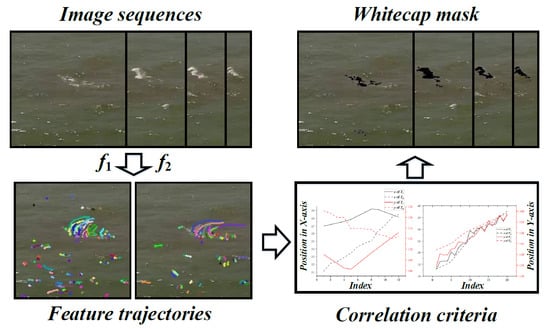
To be more precise, when only a single image is used for whitecap detection detection, it is difficult to distinguish whitecap from light pollution areas, and this is because a sun glint area behaves similarly to a whitecap. Such images could be found in Section 2.2.2, Section 3.3 and Section 3.4. Even experienced personnel find it difficult to select accurate whitecap areas from a single image when there are no other images from adjacent moments, not to mention the simple use of shape differentiation [28] or the use of brightness differences to differentiate [39]. Hence, we solve the above problems in two steps. The specific process is shown in Figure 3. First, the abnormal detection method, motivated by a previous whitecap detection method, is used for every single image in the video. The abnormal areas include whitecaps and light pollution points (where, generally, light pollution indicates sun glints). We select the channel most sensitive to abnormal pixels in the image, apply the top-hat transform to enhance the distinction between abnormal foreground and background, and use global threshold segmentation on the processed image to obtain the abnormal pixels in the image. After acquiring the most accurate abnormal areas possible, optical flow trajectories of the same features at different sampling rates are analyzed using optical flow in order to obtain the whitecaps in each image from the abnormal videos using the feature motion trajectories of light pollution and whitecaps to distinguish spurious whitecaps in the image.
2.2.1. Abnormal Detection Method
Under different illumination conditions, the brightness difference between a whitecap and the sea surface may differ greatly. Additionally, during the lifetime of a whitecap, its brightness may change [42], leading to some whitecaps potentially being ignored. Therefore, abnormal pixels are obtained under different illumination conditions for every single image in a video clip automatically. This method is abbreviated as AD (abnormal detection) in the following.
Considering that the abnormal pixels have high intensity in all channels in RGB images and light pollution points of sea surface images would have a strong specular reflection, we consider light pollution to be in the form of sun glints. The commonly used channel in specular component detection [40,43] was chosen, instead of grayscale images, as is more sensitive to sun glint points.
where R, G, and B denote the intensities of the three respective channels. In the case of different weather and different illuminations, the overall brightness and regional brightness of the image will change significantly. At this time, using a global threshold without any pre-processing is likely to cause errors. The top-hat transform has the ability to suppress the background of the image, thus enhancing the whitecaps and sun glints, which are considered as the foreground:
where denotes the top-hat transform of image I, and denotes a morphological opening applied to I, where b is the kernel used in the transform. By using a small circular kernel, background and foreground separation at different overall brightnesses can be accomplished. Figure 4a shows the effect of the top-hat transform. Background pixels are suppressed, whether they are relatively bright or dark, and abnormal pixels are enhanced, regardless of the intensity of those pixels in the original image. Figure 4b shows the intensity distribution difference after the transform, where the difference between the two histograms also confirms our observations. The histogram after the transform is smoother, and the intensity values of the background are suppressed, such that the bright background is also removed.
After the pre-processing, we can utilize the knee point in the histogram as the desired threshold T. An effective method to determine the knee point is defined as:
where denotes the variance in the number of pixels of intensity p satisfying in the statistical histogram. This method can be used in the image after the top-hat transform in order to find the threshold faster, as the threshold is closer to the origin on the x-axis and, so, the number of iterations is significantly reduced. Note that, under certain illumination conditions, there may be a small part of the sea surface that is identified as an abnormal area; however, this will not affect the subsequent analysis. Such cases could be found in Section 3.5.
2.2.2. Whitecap Separation Method
As mentioned in the previous section, with a single image, whitecaps and sun glints may have very similar appearances, as shown in Figure 5, not only in RGB space. There is only one whitecap marked, but the rest of the sun glint components are difficult to distinguish from the whitecap with limited information. In the three commonly used color spaces, the whitecap and sun glints exhibit similar color performance. An analysis of such cases could be found in Section 3.4.
Considering that the temporal and spatial characteristics of whitecaps and sun glints are different from those found in observation, they may be used to distinguish whitecaps and highlights. The specular reflection of the sea surface results in sun glints [44]. In areas where whitecaps are generated, the sea surface will not be as smooth as elsewhere, and the specular reflection component is greatly weakened, as shown in Figure 6. For sun glints, it is very related to the slope of sea surface and the distance from the camera. The overall oscillatory motion on the ocean surface is a combination of a large variety of waves [45], and the slope changes significantly at certain points on the sea surface. This makes the appearance of sun glints relatively random. With the movement of waves and currents on the sea surface, a whitecap will maintain a noticeable movement on the sea surface. Additionally, before dissipating, the whitecap areas mainly show diffuse reflection characteristics. The illumination conditions can change rapidly, and maximizing utilization of the limited available video data is important for further whitecap analysis. Instead of using a simple rule of thumb to remove suspicious components, we intend to detect whitecaps as accurately as possible through the use of spatial and temporal information. This method is abbreviated as WS (whitecap separation) in the following.
Previous methods have focused on determining the whitecap component in the image from the contour [28] itself or its duration [37], while our proposed method does not care about the contour shape, as its contour performance is quite different during the whitecap lifetime, and many kinds of shapes are possible. In practice, some specific shape contours are removed, which makes the judgment mostly dependent on experience. The proposed method is based on the analysis of optical flow trajectories at different sampling frequencies in order to determine whitecap components. Velocity measurement methods in computer vision, including particle image velocity (PIV), and optical flow methods have been applied in whitecap research [37,46], demonstrating their feasibility. In those studies, the known whitecaps were tracked to analyze the wave-breaking or the movement of whitecaps over their lifetime. Such methods are based on the prior knowledge that features in neighbor frames may correspond to each other. To track features, we utilize the L-K optical flow method [47] and use sparse optical flow to analyze all possible features.
The L-K optical flow method is based on three assumptions. (1) The brightness is constant, and the pixels of the target image in the scene do not appear to change as they move from frame to frame. For grayscale images (as well as for color images), this means that the grayscale value of the pixel does not change as the frame is tracked. (2) Temporal persistence: the movement of the camera on the image changes slowly over time. In practice, this means that changes in time do not cause drastic changes in the pixel position, such that the gray value of a pixel can be used to obtain the corresponding partial derivative with respect to the position. (3) Spatial consistency: neighboring points on the same surface in the scene have similar motions, such that their projected distances onto the image plane are also relatively close.
For speed and robustness, the input is defined as below.
where is an arbitrary point in the binary image (called a mask) obtained by threshold segmentation. The mask has the same size as the original image, and the input image retains the RGB value of the original image at if the mask value is not zero. Using the pyramid L-K optical flow function in OpenCV for calculation, a two-layer pyramid is designed, its features are obtained by the Shi–Tomasi corner detection method, and the maximum number of corner points is set to 100. The pixel corresponding to the local maximum of the first derivative (gradient of gray value) is the corner point; a detailed description of the method can be found in [48]. Figure 7 shows that when using the Shi–Tomasi corner detection method, the abnormal areas obtained by AD are used as input, and the detected corner points are distributed within the abnormal areas and on the boundary of the abnormal areas. Figure 8 shows a typical optical flow trajectory tracking case. An optical flow trajectory is a collection of the corresponding feature point positions in every frame over time, such as , where the subscript means the frame, and the maximum is 25, while represent the position on both axis. The motion trajectory between two adjacent positions is a line segment between the two points, and the smallest unit is a pixel. The optical flow trajectories are drawn in the latest image so we can see the complete trajectory of each feature point. When we utilized the image restored to WCS, the motion in the pixels also represents the motion in the plane.
Whitecaps have obvious spatial and temporal stability from the active stage to the mature stage and eventually perish [42,49,50]. Therefore, their features are distinct, and multiple stable feature points can be found in a certain whitecap contour, all of which have similar motion trajectories. According to the previous analysis, the sun glint area may not have a stable optical flow trajectory. In this way, it appears that whitecaps can be separated using optical flow trajectory analysis at a certain sampling rate. However, for sun glint areas, there may also be optical flow trajectories, and such cases are not uncommon. This is because the time interval between two neighboring frames is short, and the position and intensity of sun glint pixels may not change.
Both cases are shown in Figure 8. The time interval between each two images in the figure is 0.64 s, and 4 images are actually used to determine the optical flow trajectories between each two images. We only show the first and last two images because we want to show as much as possible the movement characteristics of the whitecap in space and time. In addition to a clearly moving whitecap, which are marked by red boxes, there are also many scattered sun glint areas, and some of them have similarities to the whitecap. In Figure 8b,c, some sun glint areas produce optical flow trajectories, and even in certain sun glint areas, multiple similar optical flow trajectories can be found.
Since, under a certain sampling rate, the sun glint areas may also result in optical flow trajectories, we propose to complete the whitecap separation through the optical flow trajectories under different sampling rates. For the more random sun glints, the corresponding feature points under different sampling rates will be quite different, which is manifested in the difference in the position of a single feature point and the difference in the overall trajectory shape on the optical flow trajectory. This phenomenon can be seen from the comparison in Figure 8b,c. Under the two sampling rates, the number of optical flow trajectories and the starting and ending positions of a single optical flow are not completely consistent. For every optical flow trajectory, the following judging criteria were designed:
(1) If stable optical flow trajectories are found at both high sampling rates and low sampling rates , we use the correlation coefficient as the criterion:
where subscript l represents sampling at , subscript h represents sampling at , T denotes the optical flow trajectory of a feature, subscript i denotes the point in T, and n is the number of points in the trajectory. is interpolated to have the same number of points as . If is higher than the design threshold, we consider the contour that obtained the trajectory point as a whitecap. Here, we set the threshold at 0.95, which means that the optical flow trajectories and are very similar.
(2) If a stable optical flow trajectory is found at only or , contours with such trajectories are simply discarded, as the feature correspondence fails.
It is difficult for us to obtain data with a higher frame rate than the original video, so the other sampling rates are derived from downsampling. For our proposed method, a variety of conditions are verified in Section 3.
3. Results
The light pollution in an image will be very different under different illumination conditions. According to the behavior and shape of the light pollution area, the performance of the proposed method under various conditions was analyzed. As mentioned above, we used videos converted to WCS. For convenience, we selected a fixed rectangular area in the videos as our region of interest (ROI), which did not change in a certain video but may differ between two videos.
3.1. Results for AD
In previous methods, images that were not pre-processed were used for whitecap detection, leading to performance that varies greatly under different illumination conditions. Here, we compare the accuracy of whitecap detection under various illumination conditions.
As shown in Figure 9, the AWE, ATS, and sub-image Otsu methods were selected for comparison with our method.
The source video of these four images was used to confirm the exact location of the whitecaps. We selected five volunteers to mark whitecaps and used the average value as the real W. The comparison between W obtained by different methods is shown in Table 1. In the first row of the figure, every method could obtain most of the whitecap areas. For AWE, the brightness of the water surface close to the whitecap is relatively high, resulting in obvious misjudgments. However, in both the ATS and sub-image Otsu(SOtsu) methods, there are missed detections. It should be noted that in Table 1, although ATS has the best effect in the first case, it is based on the fact that ATS falsely detected some whitecaps and also missed some other whitecaps. For the proposed method, the whitecaps are not missed, but only the edge of whitecaps with lower intensities are missed.
In the second row, there is almost no bright area on the water surface caused by illumination, and there is a whitecap with a significant difference in brightness from the overall water surface. In this case, all methods obtained the whitecap accurately, although AWE still obtained some misjudgments and SOtsu missed a small whitecap. Whether from the image or from the detection results, the effect of AWE and our proposed method is basically the same in this case.
In the third row, the brightness difference between the whitecap and the water surface was significantly smaller than in others. For AWE, although most of the whitecaps were obtained, many bright areas on the water surface were also misjudged. However, the threshold obtained by ATS is higher than that of AWE, and only a small part of the whitecap was obtained. This is also reflected in each case regarding the higher threshold of ATS compared to AWE, and this is the reason why the false-positive area with ATS is smaller than that of AWE. Smaller differences in brightness caused the SOtsu method to fail. In this case where the brightness difference between the whitecap and the water surface is small, through reasonable preprocessing, our method can identify the whitecap more accurately.
The last row shows the existence of many sun glints and high-brightness areas on the sea surface. In terms of the ability to detect abnormal areas, the performance of the other methods cannot be used for comparison, as this condition is not within the scope of whitecap detection; however, this condition occurs frequently. It is shown here, as minimizing the possibility of detecting high-brightness areas on the sea surface will help to speed up the performance of subsequent analyses. As can be seen in both Figure 9 and Table 1, our method is able to obtain the minimal possible abnormal sea surface. The processing time of these methods is compared in Section 3.6.2. According to the above analysis, the improved abnormal detection method proposed in this study can accurately detect whitecap and light pollution areas under different illumination conditions.
3.2. Results for WS without Sun Glint
We selected videos without light pollution conditions and applied our method in order to detect whitecaps. The original images, the optical flow trajectories under and , and the whitecap detection results are depicted in Figure 10.
In the figure, the first three and last three columns are from two different videos, which we denote by and , respectively. In the two cases, due to the different illumination conditions, the color of the sea surface is quite different, and whitecaps with different lifetimes have significant intensity differences in the same image. In , the features found were concentrated on whitecaps, with a few features on the sea surface; that is, small areas on the sea surface had relatively high brightness after the top-hat transform and were identified as abnormal areas instead of being suppressed as the background. As shown in the figure, their trajectories were not well-preserved, and thus, those features were not expected to influence further analysis. Considering the feature points of the whitecap, the number of feature points is proportional to its size; that is, the larger the whitecap, the higher the number of feature points. The whitecap marked in was undergoing a transition from the generating stage to active stage, so the whitecap area increased significantly, and feature points inside the whitecap also gradually increased. In , W is much higher than in , leading to many more feature points. All of the features were within whitecaps, as the difference between the whitecaps and the water surface was distinct. It should be noted that trajectories are not distinguished by color in order to make the difference between the trajectories more obvious, and random colors were selected for drawing.
For each whitecap, a stable optical flow trajectory can be maintained at two sampling rates. Thus, the corresponding and have high similarity. Ideally, the trajectories should be exactly the same at both sample rates, as every feature point is exactly the same. However, in the actual feature point trajectory iteration process, different feature points may be discarded or retained at different sampling rates. Therefore, we may use a spatial neighbor feature instead of the same feature. In the Shi–Tomasi corner detection method, we set the maximum number of detected corners to 100 and set the minimum distance between every two corners to 5 pixels. Both designs are based on a compromise between detection accuracy and processing speed. Both neighbor feature trajectories of and are shown in Figure 11, where and can be found in the third and sixth columns. We applied correlation analysis to the sub-trajectories in the x- and y-axes, respectively, where, in , the subscripts x and y represent the respective sub-trajectory axes.
appears as solid lines, while dashed lines represent . Changes in are not as frequent as those in , which is expected as . However, and were found to be highly correlated after linear interpolation. In addition, for a certain trajectory, too few trajectory points or the loss of features in the trajectory iterative process at may lead to the interruption of whitecap tracking. Our solution to this was as follows: once a confirmed whitecap trajectory was found, the corresponding was treated as the trajectory of the whitecap, which continued to be tracked until was lost. This is also due to consideration of the analysis speed, as if all trajectories are compared in every frame, the efficiency would be reduced. As shown in Figure 10, all whitecaps were detected in , while a few small whitecaps in were rejected, as the whitecap features were lost due to low quality.
3.3. Result of WS with Random Sun Glint
In this section, the video shown in Figure 8 was used for analysis. We used images under the WCS, while the images in Figure 8 are under the PCS. In these images, except for the whitecap, there are many sun glint pixels, which appeared and disappeared randomly, such that a stable optical flow trajectory would not exist for light pollution features. The images converted to WCS, trajectories, and whitecap detection results are provided in Figure 12. The longest trajectory lengths produced by the whitecaps and sun glints in the corresponding column are recorded in Table 2.
First, we examined the optical flow trajectory of the whitecap. In the first column of Figure 12, the whitecap is in the generating stage. Obviously, there are no and , which could be considered as neighbor feature trajectories. More precisely, the feature trajectory of the whitecap at does not build at this time. With the movement of the whitecap, the whitecap evolves into the active stage. In the second and third columns, with the update of the trajectory, stable and appear, and the length of the trajectory increases with time, as shown in Table 2, until the maximum length of 25 is reached, which indicates the existence of stable trajectories. In the last two columns, the whitecap gradually evolves from the active stage to the mature stage. In , trajectories from the active stage to the mature stage are preserved. The rapid evolution of the whitecap is hard to track at , and thus, loss of features and re-establishment of trajectories occurs, while is much shorter than in the same column. However, this does not affect the analysis, as only the last segment of trajectories at the same time period was used in the calculation of , and we only utilized , which has more points than interpolated . We assumed that interpolated has a points and has b points, where , and we used the last a points of interpolated and . What may be misleading is why the first column did not find and , which satisfy the judgment criteria, but a whitecap was still marked in Figure 12d. When we marked the whitecap in images, we assumed that we found trajectories satisfying our judgment criteria at time t, and has b points. We started processing from the image at the first point of the trajectory; that is, the image captured at time , as the number of video frames is and the contour containing the trajectory point is the whitecap.
Regarding the sun glint points, as the sun glint basically appears at random locations in such cases as in Figure 12b, except for the whitecap , there are some features brought by sun glints, some of which create light flow trajectories of a certain length. We counted the length of the longest trajectory produced by whitecaps and by sun glints in Figure 12.
Using images to describe the trajectory length is not intuitive; we describe it in more detail from the perspective of the maximum trajectory length. Based on the data in Table 2, in the first four images, is gradually increased from 4 to 25 at and from 2 to 6 at . is not stable, which also proves the random appearance of the sun glints because the length of a stable feature trajectory should be gradually accumulated. It can also be seen in Figure 12 that the trajectory of sun glints in different images vary greatly. In the fifth image, also decreases at a low sampling rate due to the transition from the active stage to the mature stage of the whitecap, but increases again in the next image. However, there is still no significant regularity in . It is also worth mentioning that the of the fourth picture at reaches 17, and with a sampling rate 25 Hz, its duration exceeds 0.67 s. According to the previous detection method [37], this area will be treated as a whitecap. Such a case is analyzed in Section 3.4.
3.4. Results for WS with Sun Glint in Certain Shapes
The condition considered in the previous section is a relatively simple case of sun glints. In more complex cases, due to the peaks and troughs of the waves, the sun glints appear to have a specific slope on the sea surface and persist with the movement of the waves. Under these conditions, the behavior and trajectories of sun glints are shown in Figure 13.
The case shown in the first three columns is denoted by , while that in the last three columns is denoted by . The marked sun glint area is similar to a whitecap in the mature stage in , but its intensity changes in a wide range, and the shape change is quite different from that of a whitecap. There is a stable trajectory at , but its corresponding does not exist. This is because, as the sampling rate decreases, the feature points that can be continuously found at are already regarded as error points in , as the feature quality threshold designed in the method will reject features with lower similarity. Hence, there are less feature points at than at . Inside the red box of , the sun glints and mature whitecaps are very hard to distinguish. On one hand, this is due to the image degradation caused by the conversion to WCS. On the other hand, the two do present very similar behaviors. The whitecap is marked in the yellow box; under the optical flow trajectory at a certain sampling rate, both whitecaps and sun glints exhibit similar persistent trajectories.
The number of trajectories and the trajectory lengths in the marked area in were compared at and , as shown in Figure 14a. In the figure, the length of the trajectories in the marked area at is longer, which is reasonable: about half of were longer than 10, and about a quarter of were longer than 16. In addition, at , a quarter of had more than 5 points. For a trajectory with a feature points at sampling rate f, the tracked time can be calculated as . In this condition, regardless of whether we use or to track the feature, if the feature lasts longer than 2/3 s, the method using tracked time [37] would fail. In the following content, we will also call it the single optical flow method, abbreviated as SOF. Correspondingly, the whitecap separation method proposed could be summarized as a method of judgment using the correlation coefficient of optical flow trajectory, which would be abbreviated as OFTC.
Figure 14.
(a) Histogram of trajectory point numbers. (b) Whitecap neighbor feature optical flow trajectories of . (c) Sun glint neighbor feature optical flow trajectories of . (d) Sun glint neighbor feature optical flow trajectories of images in Figure 15.
Figure 14.
(a) Histogram of trajectory point numbers. (b) Whitecap neighbor feature optical flow trajectories of . (c) Sun glint neighbor feature optical flow trajectories of . (d) Sun glint neighbor feature optical flow trajectories of images in Figure 15.

The whitecap trajectory and the sun glint trajectory of are shown in the figure. The correlation coefficients of the whitecap trajectory are 0.9828 and 0.9747, respectively, while the correlation coefficients of the sun glint trajectory are 0.7162 and −0.6462, respectively. The detection result of could be found in Figure 16b.
We believe that the use of optical flow trajectories at a certain sampling frequency, although temporal and spatial information is used, still lacks reliable judgment criteria. From the results in the previous section and this section, it can be seen that even the sun glint area would have a stable optical flow trajectory, and the correlation coefficient analysis at two sampling rates can solve this problem to a certain extent. Combining Figure 13 and Table 3, although there is no whitecap in , there are many light pollution areas. Obvious false detections could be found under ATS or AD. Furthermore, using SOF to remove false positives cannot remove the sun glint areas in the red box of . This is also the result of Figure 14a, as a considerable part of the feature points have long-duration optical flow trajectories. In , the information that can be obtained from the images is that the trajectories of the whitecaps and the sun glint areas are very similar, so in the actual detection results, the SOF method cannot obtain the results well.
Under WCS, the image is obviously degraded. In order to better demonstrate the sun glint with certain shape conditions, the videos under PCS were selected for the analysis, in which it is easier to distinguish between sun glints and whitecaps. In Figure 15, it is important to note that there was no whitecap in these images.
We also divided the images under PCS into two cases, and , corresponding to the first three columns and the last three columns of Figure 15, in the false detection areas by tracking the time method marked in Figure 15d. Stable optical flow trajectories can be observed at both sampling rates. We selected the last three images with more obvious trajectories, whose correlation analysis is shown in Figure 14d. The correlation coefficients were = 0.9733 and = 0.4886, respectively. The optical flow method itself depends on the brightness, and the brightness of the sun glint area varies greatly; thus, the neighbor features could be found and the stable trajectories were built, but the feature trajectories at the two sampling rates were very different. It is manifested in the results that optical flow trajectories lasts for a long time, causing significant errors. However, such errors can be removed by the proposed judgment criteria 1.
Similar to under WCS, we also compared the detection results under PCS. Due to the absence of degradation and the larger field of view, using PCS images is more likely to generate neighbor light pollution feature points on the sea surface and produce stable trajectories. The ATS and AD detection results of can refer to Figure 9, but in Figure 9, we used the third image of , and the result of AD would be higher than the second image we used here. Even though AD marked the smaller possible areas, SOF still produced significant false positives. The optical flow at two sampling rates gives more abundant information, allowingg the OFTC method to handle this condition better.
3.5. Ablation Study
It is obvious that, in the presence of sun glints, it is essential to use the optical flow method to remove misjudgments. Regardless of whether there is a whitecap in the image, only using the abnormal detection method may lead to obvious misjudgments. The images that were analyzed before are shown in Figure 16a. The top-hat transform results and the abnormal detection results indicate that the proposed abnormal detection method can identify abnormal points in the image. If the misjudgment removal method is not used, we could not retrieve a reliable W.
In Figure 16b, most of the abnormal pixels originate from light pollution. After the process of the proposed method, W can be obtained correctly. The same result can be found in Figure 12.
Even in the absence of sun glints, as mentioned above, sea surface areas with relatively high brightness in the image may also be considered abnormal areas. If the bright sea surface area is large, it can be removed using various uneven illumination correction methods; however, the smaller area itself has a similar image performance to the whitecap, and it is likely to be considered an abnormal area using the threshold segmentation method. In this case, an accurate W cannot be obtained with only a single image; the results of such cases are shown in Figure 17b. Such conditions occur very frequently. In a sea surface scene, such conditions usually last for several hours on sunny days, which is very unfavorable for long-term whitecap detection. Fortunately, it is simpler to use optical flow processing under sun glint conditions as, for sun glint points, even if the brightness of the point changes due to motion, the brightness is always much higher than the brightness of most points in the image, making the trajectory more likely to be found at high sampling rates. The general high-brightness area is only slightly brighter than other points. As time goes by, this area is not likely to exist in the following images, and the features are lost.
Considering the detection results shown in the second row in Figure 9, for example, all whitecaps were found and there were no high-brightness sea surface areas or sun glints in the image. Therefore, the whitecap detection can be accomplished without the use of subsequent processing. The trajectories after the optical flow process are shown in Figure 17c. With Figure 10, we found that the detection results would not be affected if we added the optical flow method. The process is not required under such conditions; however, there is no good way to automatically determine whether the image contains sun glints and high-brightness sea surface areas. According to a previous statistical analysis of whitecaps [51], we can estimate the approximate range of W at the current wind speed based on statistical information. However, this method is still not stable because there may still be a notable difference from the empirical curve in actual situations.
3.6. Comparison with Previous Method
3.6.1. Accuracy Comparison
Due to in situ storage limitations at sea and the filtering of available video data, our data are mainly derived from in the range of 5–10 m/s; this can be observed from Figure 1b. In the existing dataset, firstly, we consider the use of videos without light pollution to obtain the widely used 20-min whitecap coverage W [19,52,53]. Both W obtained using ATS and using AD are displayed. We used ATS and AD in the same dataset, and the results showed that the differences were not significant. In Figure 18, we added the experience curve proposed by Scanlon [52], and most of the W we obtained is below the convex curve. Although we cannot confirm that the statistical characteristics of the whitecap in the current sea area and utilized in Scanlon’s work are the same, we could use it as a rough distinction criterion. In our dataset, the value of W at the most time should be lower than that obtained from the curve at a certain or close to it.
It needs to be explained that since the camera is not toward the nadir, it is inevitable that, at certain moments, part of the whitecap will be obscured by the wave crest that is closer to the camera, which may result in a smaller W obtained. In our verification, we found the phenomenon has a very limited impact on results. On the one hand, we used a 20-min average of the whitecap coverage, and errors in a small number of images are tolerable. On the other hand, the occlusion is not particularly severe due to the used part in the original image, as shown by the orange box in Figure 2b.
Furthermore, we selected the videos under different light pollution conditions and plotted W obtained by (1) the SOF method, (2) the proposed OFTC method, and (3) the whitecap extraction method using single image in Figure 18. It is obvious that in the results without using video data, W has a great error due to the influence of illumination and has little relationship with wind speed. The method using tracked time can obtain results close to the optical flow correlation coefficient method in some cases, such as case A in the figure. However, in case B, the single optical flow method still cannot obtain reliable results. This actually has much to do with the shape of light pollution. As previously introduced in Section 3.3 and Section 3.4, case A and case B are obtained from videos of different light pollution shapes, and if the shape of a sun glint area is similar to a whitecap shape, the performance of SOF will be greatly attenuated. In the results of case B, the W obtained by the SOF method is also several times higher than the statistical data. Since the ordinate of Figure 18 is logarithmic, a slightly larger value also represents a difference of several times, not to mention that the SOF results in case B are significantly far from the statistical value. While the results obtained by the OFTC method are relatively more reliable, our proposed method can guarantee almost the same accuracy as previous methods in the case of random light pollution and can still stably extract the whitecap of the sea surface in the case of specific-shaped light pollution.
3.6.2. Processing Time Comparison
According to the above analysis, we believe that, under various illumination conditions and with only video data available, the proposed post-processing method should be widely used rather than only relying on single-image information. Videos under different illumination conditions were selected for process time analysis. All codes used were written in Python. Figure 19 shows the processing times of the abnormal detection method and the abnormal detection method + whitecap separation method compared to those of methods available in the literature.
Due to the multiple derivation and smoothing operations of AWE, its algorithm efficiency is relatively low, while ATS, the sub-image Otsu method, and the proposed abnormal detection method can be processed quickly. After fixing the image size, these methods are not concerned with the content of the image, which makes their process efficiency basically fixed. However, after adding post-processing, the processing speed will be significantly reduced. First, the optical flow trajectory acquisition under two sampling rates will lead to reduced performance. In addition, the neighbor feature correspondence and correlation were calculated after the trajectory, which also reduces the processing speed. The video we selected include sea states with relatively low W, relatively high W, whitecaps and sun glint points, as well as whitecaps and large sun glint areas, corresponding to 0–500, 500–1000, 1000–1500 frames, and >1500 frames, respectively. Images from this video are shown above, for example, in Figure 8 and Figure 9. In these cases, the number of feature points in the images differ, resulting in different feature trajectories that need to be judged. Therefore, it can be seen that the processing time after 500 frames was significantly longer than that before 500 frames. Except for relatively low W, there will be many abnormal areas in the images causing many feature points, especially in the case of large sun glint areas, and therefore, the required processing time increased significantly. In the first stage of processing (about 25 frames), AD+WS ran significantly faster than in the subsequent frames, as the whitecap that is not detected in the current frame needs to be fully considered. In this way, there will not be a single whitecap that goes undetected. Before 25 frames, the program only needs to store the pictures into the queue while, after 25 frames, it starts to perform enqueue and dequeue operations and detects the whitecap(s) in each frame, which would take a relatively greater amount of time. However, in general, the time required for AD+WS is acceptable, and the detection could be completed in real-time.
4. Discussion
In previous work on whitecap detection, the inefficiency of manual marking led to research on the automated detection of whitecaps. Notably, in the automated extraction process, due to the influence of illumination, failure to perform error correction due to light pollution can lead to significant detection errors. Currently popular single-image post-processing approaches are generally based on contours, but this relies on strong prior knowledge. From the data in this study, we can state that there are obvious differences in the shapes of whitecaps; therefore, utilizing contours to determine the presence of a whitecap is difficult. Another type of method is based on brightness difference. Although there is a certain brightness difference between light pollution and certain whitecaps, whitecaps in different lifetimes also have obvious brightness differences. In general, the information that can be utilized to separate whitecaps from light pollution areas in a single image is very limited, and manual marking is difficult to achieve under such a condition. Furthermore, in previous studies, few illumination conditions are considered, and whether the method can be used under various illuminations could not be proved.
Therefore, the detection of whitecaps should not only be limited to a single image; instead, the presence or absence of whitecaps should be confirmed using video data. Whitecaps are an important part of the air–sea exchange, and they can last on the sea surface for some time. Moreover, whitecaps are displaced with the waves and currents, which is significantly different from the sun glints we observed. Manual marking can often obtain accurate whitecaps in a video sequence, but when the video sequence is not available and the illumination pollution is strong, recognizing whitecaps can be difficult even for humans. Considering the movement of a whitecap, a method using the tracked time to judge the whitecap was proposed, but only judging by time can lead to some long-lasting light-pollution areas also being marked as whitecaps.
The abnormal detection method proposed in the study was motivated by previous research [19,23,27,43]. Using the channel makes our method more sensitive to the points with specular reflection in the image, and using the top-hat transform also makes it possible to suppress the larger bright background in the image. Furthermore, a new histogram-based threshold determination method is used, which simplifies the search process and improves the robustness of the approach, compared to previous ones requiring derivation and smoothing operations. Under different illumination conditions, the whitecap detection accuracy is higher, and the determination of abnormal points under strong illumination pollution is more accurate. Under different illumination conditions, the proposed abnormal detection method was shown to be able to detect whitecaps more accurately in images without light pollution than previous whitecap detection methods. In the images containing light pollution, our method could detect all possible areas that may contain whitecaps. Compared with the previous whitecap detection method, we reduced the candidate area as much as possible to improve the speed of subsequent analysis.
In the analysis of whitecaps under different illumination conditions, the post-processing method proposed in this study does not concern the shape of the contour and only judges whether the contour is a whitecap or not by assessing the correlation of the motion trajectories of neighboring feature points under the high and low sampling rates, making the proposed method much less dependent on experience. Compared with the tracked time method, the illumination pollution component can be removed more accurately. In addition, compared with previous research, the premise of this method is the use of a high video sampling rate, while the low sampling rate used in this paper is the same as the sampling rate in most previous studies. It should be noted that this study is still based on prior knowledge, as the randomness of sun glints appearing and disappearing allows us to find different feature trajectories for the same sun glint features at different sampling rates, while whitecap features are obviously spatially and temporally continuous.
The method proposed in this study also has limitations. First, for a large W, the abnormal detection method will fail, which is the same as observed in previous whitecap detection methods based on thresholds retrieved from histograms. In post-processing, illumination pollution can be removed in most cases; however, the brightness uniformity of some sun glint areas is good and the sun glint area features last for a long time in a manner closely related to the current wave shape and sea state. In future work, we will focus on solving this problem. It is also worth mentioning that using the motion detection method of computer vision to analyze the movement of whitecaps is also a problem worthy of study, which can be used to distinguish the lifetime of a certain whitecap [14,46,50,54], and deepen the understanding of the role of whitecaps in different lifetimes [52,55,56]. The method proposed in this study, while removing illumination pollution, actually includes many trajectories of whitecap movement over time. Tracking specific whitecaps and analyzing the movement of whitecaps in different stages could be a main research direction in future work.
Author Contributions
Conceptualization, M.L. and X.H.; methodology, X.H.; software, X.H.; validation, C.H.; formal analysis, M.L. and Q.Y.; investigation, C.H. and A.M.; resources, Q.Y. and A.M.; data curation, Q.Y.; writing—original draft preparation, X.H.; writing—review and editing, M.L., Q.Y. and S.C.; visualization, C.H. and A.M.; supervision, M.L.; project administration, M.L.; funding acquisition, M.L. and S.C. All authors have read and agreed to the published version of the manuscript.
Funding
This research was funded by the Shandong Provincial Key Research and Development Program (SPKR&DP-MSTIP; 2019JZZY010902), The Major Scientific and Technological Innovation Project of Shandong Province (2021ZLGX04) and The Taishan Scholars Program of Shandong Province: No. ts20190914.
Data Availability Statement
Data underlying the results presented in this paper are not publicly available at this time, but may be obtained from the authors upon reasonable request.
Conflicts of Interest
The authors declare no conflict of interest.
References
- Monahan, E.C.; Spillane, M.C. The role of oceanic whitecaps in air-sea gas exchange. In Gas Transfer at Water Surfaces; Springer: Berlin/Heidelberg, Germany, 1984; pp. 495–503. [Google Scholar]
- Wanninkhof, R.; Asher, W.E.; Ho, D.T.; Sweeney, C.; McGillis, W.R. Advances in quantifying air-sea gas exchange and environmental forcing. Annu. Rev. Mar. Sci. 2009, 1, 213–244. [Google Scholar] [CrossRef] [PubMed] [Green Version]
- Mårtensson, E.; Nilsson, E.; de Leeuw, G.; Cohen, L.; Hansson, H.C. Laboratory simulations and parameterization of the primary marine aerosol production. J. Geophys. Res. Atmos. 2003, 108. [Google Scholar] [CrossRef] [Green Version]
- Stabeno, P.; Monahan, E. The influence of whitecaps on the albedo of the sea surface. In Oceanic Whitecaps; Springer: Berlin/Heidelberg, Germany, 1986; pp. 261–266. [Google Scholar]
- Koepke, P. Effective reflectance of oceanic whitecaps. Appl. Opt. 1984, 23, 1816–1824. [Google Scholar] [CrossRef] [PubMed] [Green Version]
- Bobak, J.P.; Asher, W.E.; Dowgiallo, D.J.; Anguelova, M.D. Aerial radiometric and video measurements of whitecap coverage. IEEE Trans. Geosci. Remote Sens. 2011, 49, 2183–2193. [Google Scholar] [CrossRef]
- Callaghan, A.H.; Deane, G.B.; Stokes, M.D. Two regimes of laboratory whitecap foam decay: Bubble-plume controlled and surfactant stabilized. J. Phys. Oceanogr. 2013, 43, 1114–1126. [Google Scholar] [CrossRef]
- Schwendeman, M.; Thomson, J. Observations of whitecap coverage and the relation to wind stress, wave slope, and turbulent dissipation. J. Geophys. Res. Ocean. 2015, 120, 8346–8363. [Google Scholar] [CrossRef]
- Liu, M.; Yang, B.; Jia, N.; Zou, Z. Dependence of estimating whitecap coverage on currents and swells. J. Ocean. Univ. China 2021, 20, 512–520. [Google Scholar] [CrossRef]
- Pivaev, P.D.; Kudryavtsev, V.N.; Korinenko, A.E.; Malinovsky, V.V. Field observations of breaking of dominant surface waves. Remote Sens. 2021, 13, 3321. [Google Scholar] [CrossRef]
- Peach, J.; Callaghan, A.; Bergamasco, F.; Benetazzo, A.; Barbariol, F. Detection and Tracking of Individual Surface Breaking Waves From a Fixed Stereo Video System; Technical Report; Copernicus Meetings: Vienna, Austria, 2022. [Google Scholar]
- Buscombe, D.; Carini, R.J. A data-driven approach to classifying wave breaking in infrared imagery. Remote Sens. 2019, 11, 859. [Google Scholar] [CrossRef] [Green Version]
- Dierssen, H.M. Hyperspectral measurements, parameterizations, and atmospheric correction of whitecaps and foam from visible to shortwave infrared for ocean color remote sensing. Front. Earth Sci. 2019, 7, 14. [Google Scholar] [CrossRef]
- Potter, H.; Smith, G.B.; Snow, C.M.; Dowgiallo, D.J.; Bobak, J.P.; Anguelova, M.D. Whitecap lifetime stages from infrared imagery with implications for microwave radiometric measurements of whitecap fraction. J. Geophys. Res. Ocean. 2015, 120, 7521–7537. [Google Scholar] [CrossRef]
- Santos-Ferreira, A.M.; da Silva, J.C.; Magalhaes, J.M.; Amraoui, S.; Moreau, T.; Maraldi, C.; Boy, F.; Picot, N.; Borde, F. Effects of Surface Wave Breaking Caused by Internal Solitary Waves in SAR Altimeter: Sentinel-3 Copernicus Products and Advanced New Products. Remote Sens. 2022, 14, 587. [Google Scholar] [CrossRef]
- Anguelova, M.D.; Webster, F. Whitecap coverage from satellite measurements: A first step toward modeling the variability of oceanic whitecaps. J. Geophys. Res. Ocean. 2006, 111. [Google Scholar] [CrossRef] [Green Version]
- Anguelova, M.D.; Bettenhausen, M.H. Whitecap fraction from satellite measurements: Algorithm description. J. Geophys. Res. Ocean. 2019, 124, 1827–1857. [Google Scholar] [CrossRef]
- Ren, D.; Hua, F.; Yang, Y.; Sun, B. The improved model of estimating global whitecap coverage based on satellite data. Acta Oceanol. Sin. 2016, 35, 66–72. [Google Scholar] [CrossRef]
- Callaghan, A.H.; White, M. Automated processing of sea surface images for the determination of whitecap coverage. J. Atmos. Ocean. Technol. 2009, 26, 383–394. [Google Scholar] [CrossRef]
- Massouh, L.; Le Calve, O. Measurement of whitecap coverage during FETCH 98 experiment. J. Aerosol Sci. 1999, 30, 177–178. [Google Scholar] [CrossRef]
- Lafon, C.; Piazzola, J.; Forget, P.; Le Calve, O.; Despiau, S. Analysis of the variations of the whitecap fraction as measured in a coastal zone. Bound.-Layer Meteorol. 2004, 111, 339–360. [Google Scholar] [CrossRef]
- Sugihara, Y.; Tsumori, H.; Ohga, T.; Yoshioka, H.; Serizawa, S. Variation of whitecap coverage with wave-field conditions. J. Mar. Syst. 2007, 66, 47–60. [Google Scholar] [CrossRef]
- Bakhoday-Paskyabi, M.; Reuder, J.; Flügge, M. Automated measurements of whitecaps on the ocean surface from a buoy-mounted camera. Methods Oceanogr. 2016, 17, 14–31. [Google Scholar] [CrossRef]
- Eadi Stringari, C.; Veras Guimarães, P.; Filipot, J.F.; Leckler, F.; Duarte, R. Deep neural networks for active wave breaking classification. Sci. Rep. 2021, 11, 3604. [Google Scholar] [CrossRef] [PubMed]
- Saez, F.J.; Catalan, P.A.; Valle, C. Wave-by-wave nearshore wave breaking identification using U-Net. Coast. Eng. 2021, 170, 104021. [Google Scholar] [CrossRef]
- Wang, Y.; Sugihara, Y.; Zhao, X.; Nakashima, H.; Eljamal, O. Deep Learning-Based Image Processing for Whitecaps on the Ocean Surface. J. Jpn. Soc. Civ. Eng. Ser. B2 (Coast. Eng.) 2020, 76, 163–168. [Google Scholar] [CrossRef]
- Liu, X.; Zhang, S.; Li, M.; Dang, C. Study on Comparison, Improvement and Application of Whitecap Automatic Identification Algorithm. Semicond. Optoelectron. 2017, 38, 758–761. [Google Scholar]
- Al-Lashi, R.S.; Webster, M.; Gunn, S.R.; Czerski, H. Toward omnidirectional and automated imaging system for measuring oceanic whitecap coverage. J. Opt. Soc. Am. A 2018, 35, 515–521. [Google Scholar] [CrossRef]
- Zhao, H.; Ji, Z.; Zhang, Y.; Sun, X.; Song, P.; Li, Y. Mid-infrared imaging system based on polarizers for detecting marine targets covered in sun glint. Opt. Express 2016, 24, 16396–16409. [Google Scholar] [CrossRef]
- Remondino, F.; Fraser, C. Digital camera calibration methods: Considerations and comparisons. Int. Arch. Photogramm. Remote Sens. Spat. Inf. Sci. 2006, 36, 266–272. [Google Scholar]
- Ottaviani, M.; Spurr, R.; Stamnes, K.; Li, W.; Su, W.; Wiscombe, W. Improving the description of sunglint for accurate prediction of remotely sensed radiances. J. Quant. Spectrosc. Radiat. Transf. 2008, 109, 2364–2375. [Google Scholar] [CrossRef]
- Wang, M.; Bailey, S.W. Correction of sun glint contamination on the SeaWiFS ocean and atmosphere products. Appl. Opt. 2001, 40, 4790–4798. [Google Scholar] [CrossRef]
- Mustard, J.F.; Staid, M.I.; Fripp, W.J. A semianalytical approach to the calibration of AVIRIS data to reflectance over water: Application in a temperate estuary. Remote Sens. Environ. 2001, 75, 335–349. [Google Scholar] [CrossRef]
- Martin, J.; Eugenio, F.; Marcello, J.; Medina, A. Automatic sun glint removal of multispectral high-resolution WorldView-2 imagery for retrieving coastal shallow water parameters. Remote Sens. 2016, 8, 37. [Google Scholar] [CrossRef] [Green Version]
- Muslim, A.M.; Chong, W.S.; Safuan, C.D.M.; Khalil, I.; Hossain, M.S. Coral reef mapping of UAV: A comparison of sun glint correction methods. Remote Sens. 2019, 11, 2422. [Google Scholar] [CrossRef]
- Wang, G.; Wang, J.; Zhang, Z.; Cui, B. Performance of eliminating sun glints reflected off wave surface by polarization filtering under influence of waves. Optik 2016, 127, 3143–3149. [Google Scholar] [CrossRef]
- Kleiss, J.M.; Melville, W.K. The analysis of sea surface imagery for whitecap kinematics. J. Atmos. Ocean. Technol. 2011, 28, 219–243. [Google Scholar] [CrossRef]
- Vrecica, T.; Paletta, Q.; Lenain, L. Deep learning applied to sea surface semantic segmentation: Filtering sunglint from aerial imagery. In Proceedings of the ICML 2021 Workshop on Tackling Climate Change with Machine Learning, Online, 23 July 2020. [Google Scholar]
- Yurovsky, Y.Y.; Kudryavtsev, V.N.; Grodsky, S.A.; Chapron, B. Ka-band radar cross-section of breaking wind waves. Remote Sens. 2021, 13, 1929. [Google Scholar] [CrossRef]
- Shen, H.L.; Zheng, Z.H. Real-time highlight removal using intensity ratio. Appl. Opt. 2013, 52, 4483–4493. [Google Scholar] [CrossRef] [Green Version]
- Zhang, Z. A flexible new technique for camera calibration. IEEE Trans. Pattern Anal. Mach. Intell. 2000, 22, 1330–1334. [Google Scholar] [CrossRef] [Green Version]
- Monahan, E.C.; Wodlf, D.; Wu, J. Comments on “Variations of whitecap coverage with wind stress and water temperature”. J. Phys. Oceanogr. 1989, 19, 706–711. [Google Scholar] [CrossRef]
- Kim, H.; Jin, H.; Hadap, S.; Kweon, I. Specular reflection separation using dark channel prior. In Proceedings of the IEEE Conference on Computer Vision and Pattern Recognition, Portland, OR, USA, 23–28 June 2013; pp. 1460–1467. [Google Scholar]
- Kay, S.; Hedley, J.D.; Lavender, S. Sun glint correction of high and low spatial resolution images of aquatic scenes: A review of methods for visible and near-infrared wavelengths. Remote Sens. 2009, 1, 697–730. [Google Scholar] [CrossRef] [Green Version]
- Toffoli, A.; Bitner-Gregersen, E.M. Types of ocean surface waves, wave classification. Encycl. Marit. Offshore Eng. 2017, 1–8. [Google Scholar] [CrossRef]
- Yang, X.; Potter, H. A Novel Method to Discriminate Active from Residual Whitecaps Using Particle Image Velocimetry. Remote Sens. 2021, 13, 4051. [Google Scholar] [CrossRef]
- Lucas, B.D.; Kanade, T. An iterative image registration technique with an application to stereo vision. In Proceedings of the 7th International Joint Conference on Artificial Intelligence (IJCAI ’81), Vancouver, BC, Canada, 24–28 August 1981; Volume 81. [Google Scholar]
- Shi, J. Good features to track. In Proceedings of the 1994 IEEE Conference on Computer Vision and Pattern Recognition, Seattle, WA, USA, 21–23 June 1994; pp. 593–600. [Google Scholar]
- Callaghan, A.H.; Deane, G.B.; Stokes, M.D.; Ward, B. Observed variation in the decay time of oceanic whitecap foam. J. Geophys. Res. Ocean. 2012, 117. [Google Scholar] [CrossRef]
- Scanlon, B.; Ward, B. Oceanic wave breaking coverage separation techniques for active and maturing whitecaps. Methods Oceanogr. 2013, 8, 1–12. [Google Scholar] [CrossRef]
- Vlahos, P.; Monahan, E.C. Recent Advances in the Study of Oceanic Whitecaps: Twixt Wind and Waves; Springer Nature: Berlin/Heidelberg, Germany, 2020. [Google Scholar]
- Scanlon, B.; Ward, B. The influence of environmental parameters on active and maturing oceanic whitecaps. J. Geophys. Res. Ocean. 2016, 121, 3325–3336. [Google Scholar] [CrossRef] [Green Version]
- Brumer, S.E.; Zappa, C.J.; Brooks, I.M.; Tamura, H.; Brown, S.M.; Blomquist, B.W.; Fairall, C.W.; Cifuentes-Lorenzen, A. Whitecap coverage dependence on wind and wave statistics as observed during SO GasEx and HiWinGS. J. Phys. Oceanogr. 2017, 47, 2211–2235. [Google Scholar] [CrossRef]
- Mironov, A.S.; Dulov, V.A. Detection of wave breaking using sea surface video records. Meas. Sci. Technol. 2007, 19, 015405. [Google Scholar] [CrossRef]
- Monahan, E.C.; Zietlow, C.R. Laboratory comparisons of fresh-water and salt-water whitecaps. J. Geophys. Res. 1969, 74, 6961–6966. [Google Scholar] [CrossRef]
- Anguelova, M.D.; Hwang, P.A. Using energy dissipation rate to obtain active whitecap fraction. J. Phys. Oceanogr. 2016, 46, 461–481. [Google Scholar] [CrossRef]
Figure 1.
(a) Instrumentation; (b) wind speed and significant wave height data in video clips analyzed in this study.
Figure 1.
(a) Instrumentation; (b) wind speed and significant wave height data in video clips analyzed in this study.

Figure 2.
(a) The spatial location of the WCS and the PCS. (b) The original image taken by the camera and the image restored to WCS. The orange box marks the area restored to WCS, and the orange points in two images are the corresponding positions of the origin coordinate in the WCS. The spatial size of the image under the WCS is 50.00 m × 85.69 m, with the same spatial resolution in both axes.

Figure 3.
Flowchart of the proposed method.

Figure 4.
(a) The original grayscale image and the image after top-hat transformation; (b) histogram of image before and after the top-hat transform. The dashed line represents the threshold found by the knee point determination method.
Figure 4.
(a) The original grayscale image and the image after top-hat transformation; (b) histogram of image before and after the top-hat transform. The dashed line represents the threshold found by the knee point determination method.

Figure 5.
(a) Image containing sun glints and whitecap in RGB color space; (b) image containing sun glints and whitecap in HSV color space; and (c) image containing sun glints and whitecap in LAB color space (the display colors of this image have been modified to enhance the difference).
Figure 5.
(a) Image containing sun glints and whitecap in RGB color space; (b) image containing sun glints and whitecap in HSV color space; and (c) image containing sun glints and whitecap in LAB color space (the display colors of this image have been modified to enhance the difference).

Figure 6.
Schematic diagram of water surface reflection. In the case of A, C, D, and E, specular reflection is dominant, and A, D, and E may all have sun glints in the result. In case B, diffuse reflection is dominant due to the occurrence of whitecaps.
Figure 6.
Schematic diagram of water surface reflection. In the case of A, C, D, and E, specular reflection is dominant, and A, D, and E may all have sun glints in the result. In case B, diffuse reflection is dominant due to the occurrence of whitecaps.

Figure 7.
(a) Original image; (b) input image for Shi–Tomasi corner detection. (c) The features found by Shi–Tomasi corner detection.
Figure 7.
(a) Original image; (b) input image for Shi–Tomasi corner detection. (c) The features found by Shi–Tomasi corner detection.

Figure 8.
(a) Original video. (b) The corresponding optical flow trajectory at one sampling rate. The interval between two images is 0.64 s. (c) The corresponding optical flow trajectory at the other sampling rate.
Figure 8.
(a) Original video. (b) The corresponding optical flow trajectory at one sampling rate. The interval between two images is 0.64 s. (c) The corresponding optical flow trajectory at the other sampling rate.

Figure 9.
(a) Original images; (b) whitecap obtained using AWE; (c) whitecap obtained using ATS; (d) whitecap obtained using the sub-image Otsu method; and (e) whitecap obtained using the proposed method.
Figure 9.
(a) Original images; (b) whitecap obtained using AWE; (c) whitecap obtained using ATS; (d) whitecap obtained using the sub-image Otsu method; and (e) whitecap obtained using the proposed method.

Figure 10.
(a) Original images where the interval between two images is 0.16 s; (b) at 25 Hz. Within , the trajectories were updated 4 times; (c) at 6.25 Hz. Within , the trajectories were only updated 1 time; and (d) whitecap retrieval result using our method under no sun glint conditions. Whitecap areas are shown as black pixels.

Figure 11.
(a) Neighbor feature trajectories at and in with the horizontal ordinate Index represents the ith point in this optical flow trajectory, . (b) Neighbor feature trajectories at and in with .
Figure 11.
(a) Neighbor feature trajectories at and in with the horizontal ordinate Index represents the ith point in this optical flow trajectory, . (b) Neighbor feature trajectories at and in with .

Figure 12.
(a) Original images under WCS. is not fixed, as the entire whitecap lifetime is to be displayed; (b) at 25 Hz; (c) at 6.25 Hz; and (d) whitecap retrieval results using our method under no sun glint conditions. Whitecap areas are shown as black pixels.
Figure 12.
(a) Original images under WCS. is not fixed, as the entire whitecap lifetime is to be displayed; (b) at 25 Hz; (c) at 6.25 Hz; and (d) whitecap retrieval results using our method under no sun glint conditions. Whitecap areas are shown as black pixels.

Figure 13.
(a) Original images for two videos. Three images were taken from each video. s; (b) ; and (c) .
Figure 13.
(a) Original images for two videos. Three images were taken from each video. s; (b) ; and (c) .

Figure 15.
(a) Original images; (b) ; (c) ; and (d) false-positive areas caused by using only tracked time.
Figure 15.
(a) Original images; (b) ; (c) ; and (d) false-positive areas caused by using only tracked time.

Figure 16.
(a) The top-hat transform and abnormal detection results of sun glints in Figure 15 and ; and (b) the whitecap separation process, from the original image to top-hat transform result and abnormal detection result and, finally, to the whitecap separation result in .
Figure 16.
(a) The top-hat transform and abnormal detection results of sun glints in Figure 15 and ; and (b) the whitecap separation process, from the original image to top-hat transform result and abnormal detection result and, finally, to the whitecap separation result in .

Figure 17.
(a) The high-brightness sea surface, considered as abnormal with, ; (b) the abnormal area of (a), marked with black pixels; and (c) whitecap trajectories without any illumination pollution at and of the second row in Figure 9. .
Figure 17.
(a) The high-brightness sea surface, considered as abnormal with, ; (b) the abnormal area of (a), marked with black pixels; and (c) whitecap trajectories without any illumination pollution at and of the second row in Figure 9. .

Figure 18.
W obtained by different methods. No sun glint ATS represents W obtained using the ATS method without light pollution, no sun glint AD represents W obtained using the AD we proposed without light pollution, AD represents W obtained by whitecap extraction method using only a single image, SOF represents W obtained by single optical flow method, and OFTC represents W obtained by the optical flow trajectories correlation method.

Figure 19.
Comparison of processing time of different methods. Note: AD, proposed abnormal detection method; AD+WS, proposed abnormal detection method + proposed whitecap separation method; SOtsu, sub-image Otsu method.
Figure 19.
Comparison of processing time of different methods. Note: AD, proposed abnormal detection method; AD+WS, proposed abnormal detection method + proposed whitecap separation method; SOtsu, sub-image Otsu method.


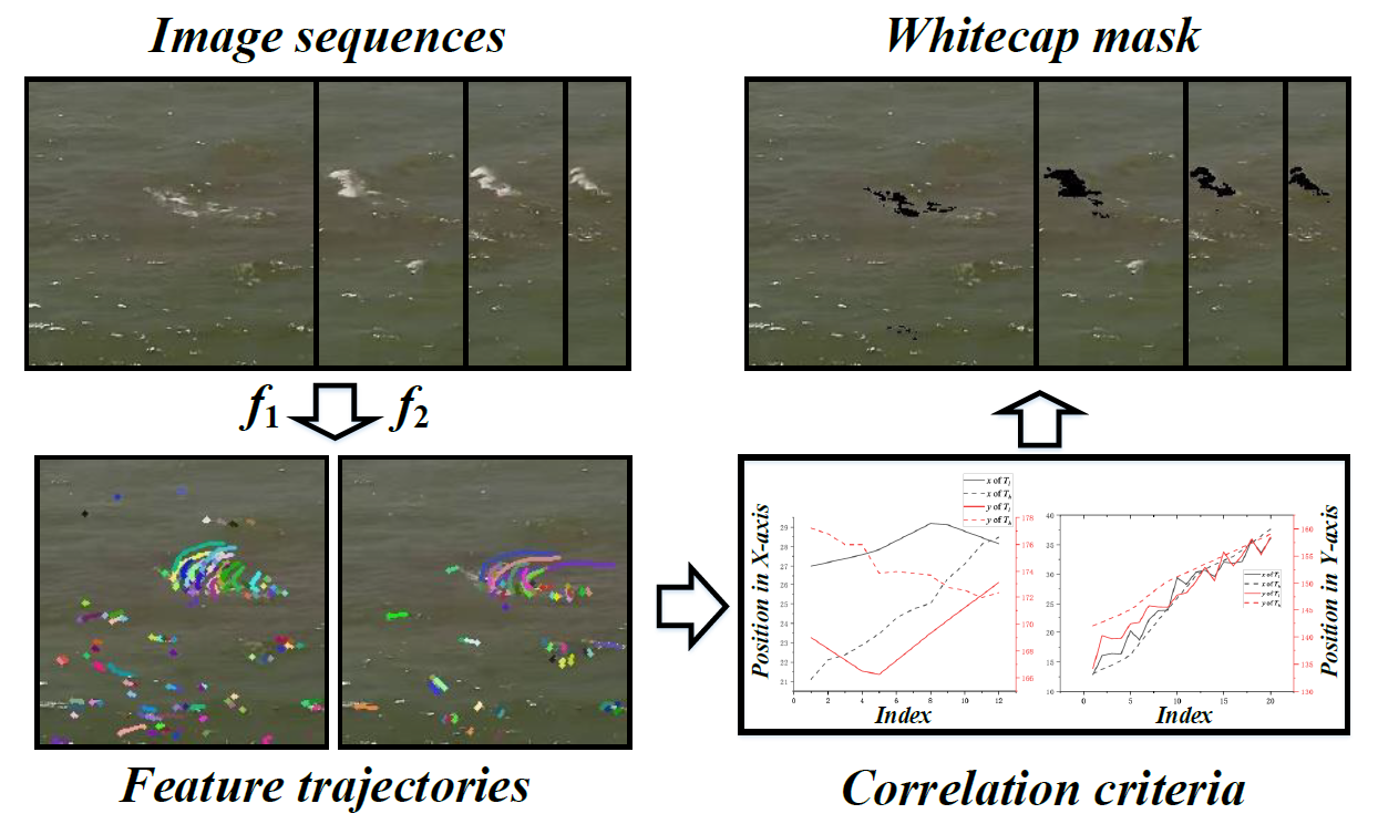
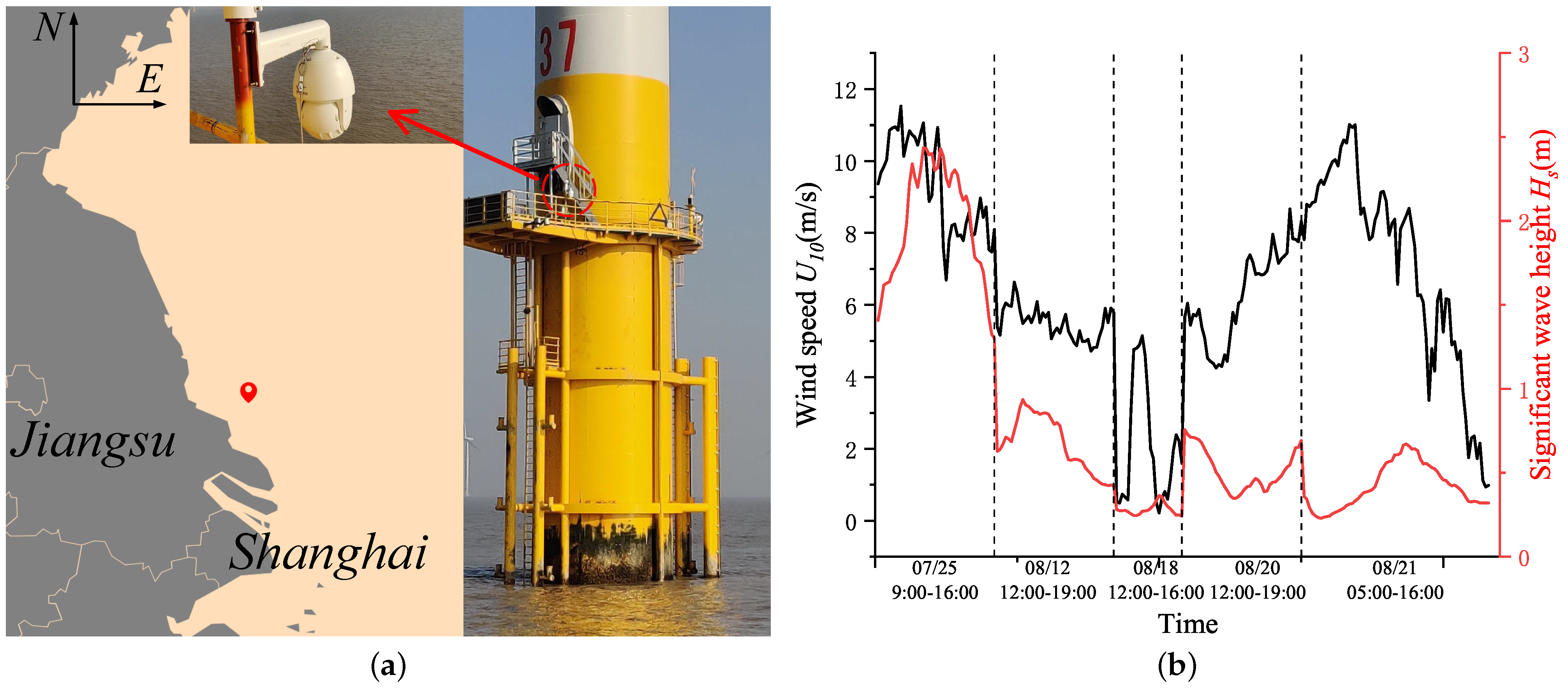
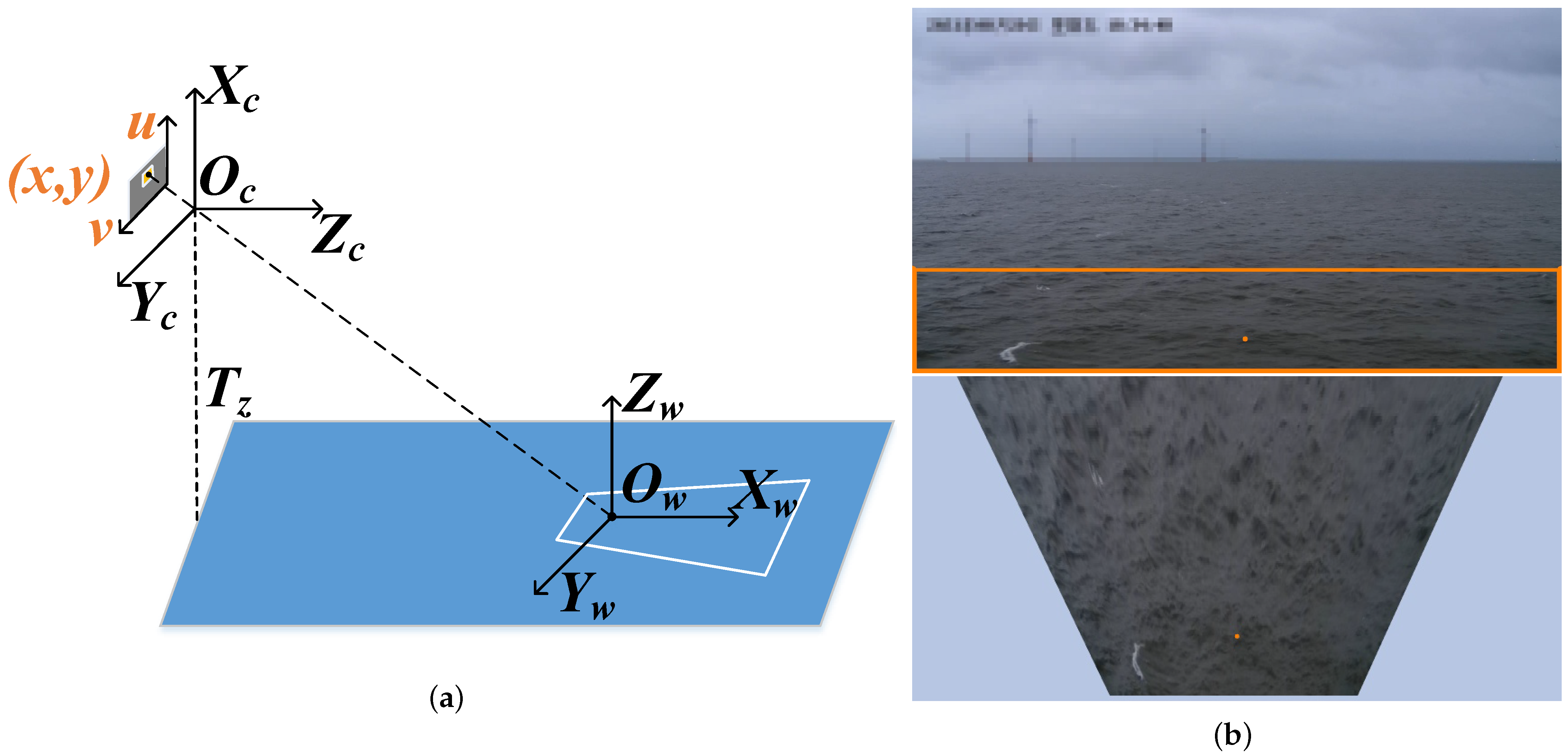
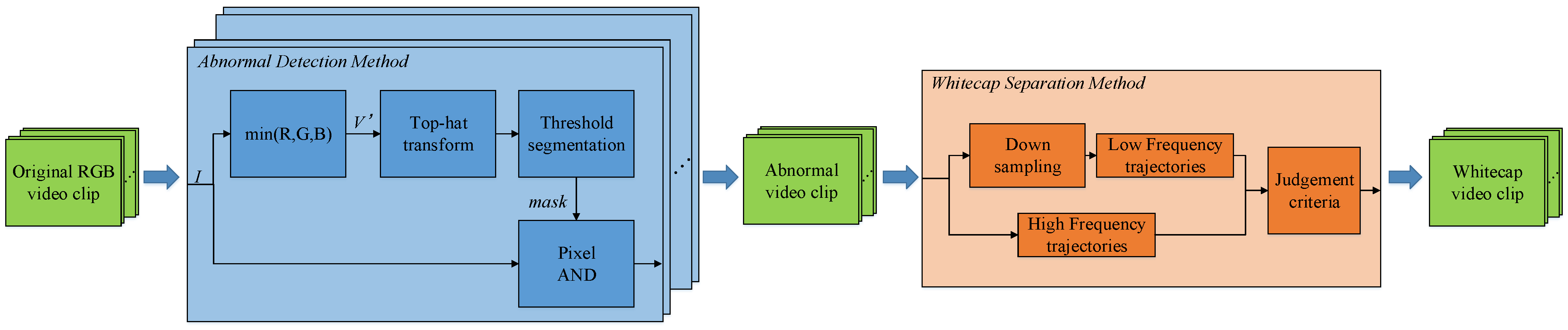
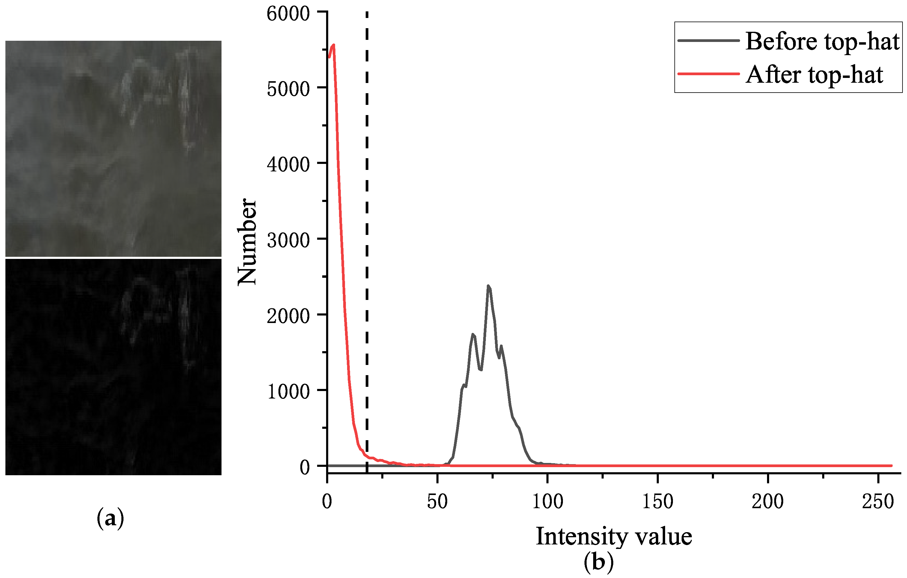
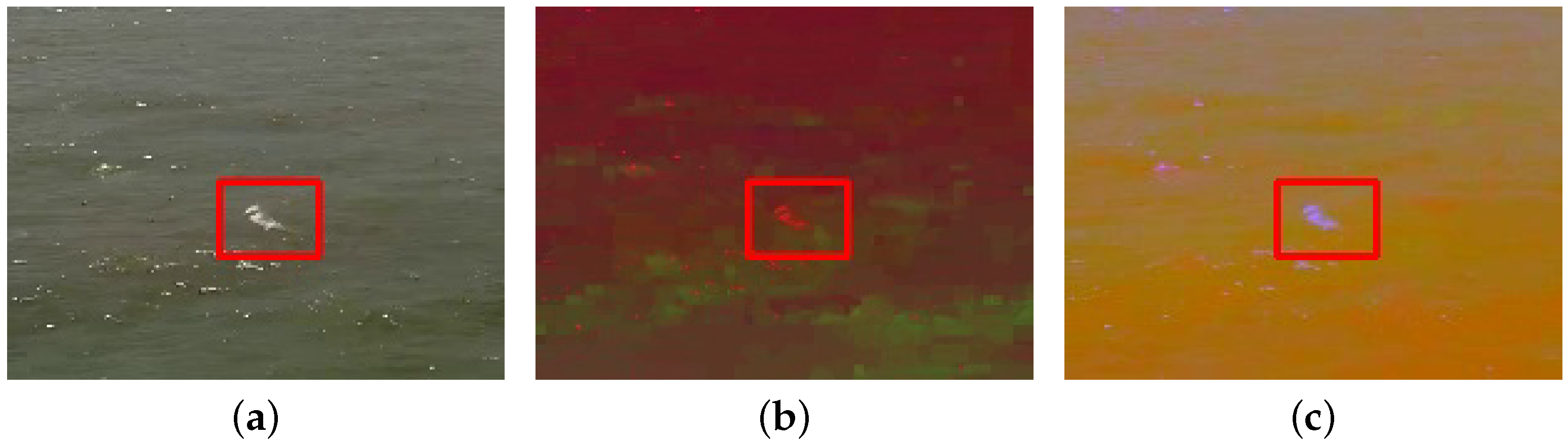
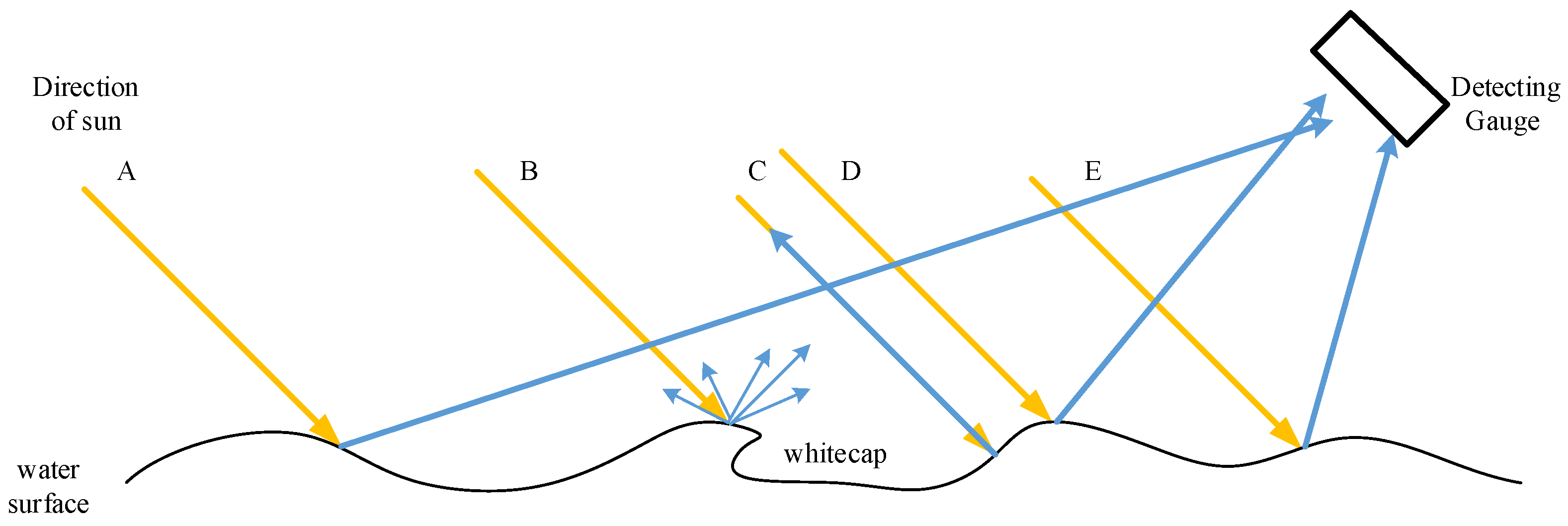
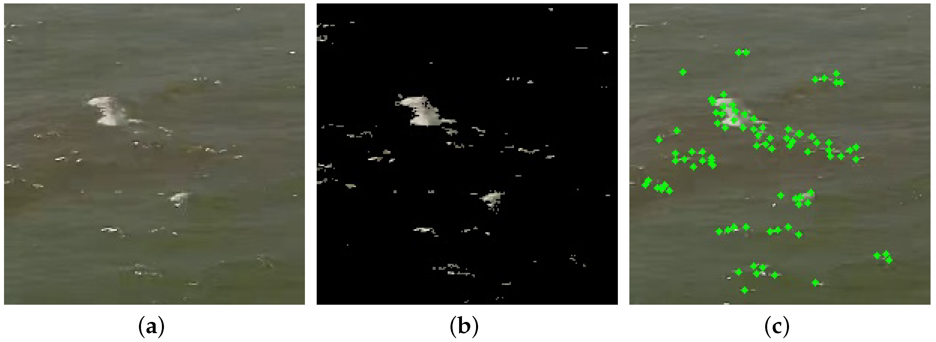
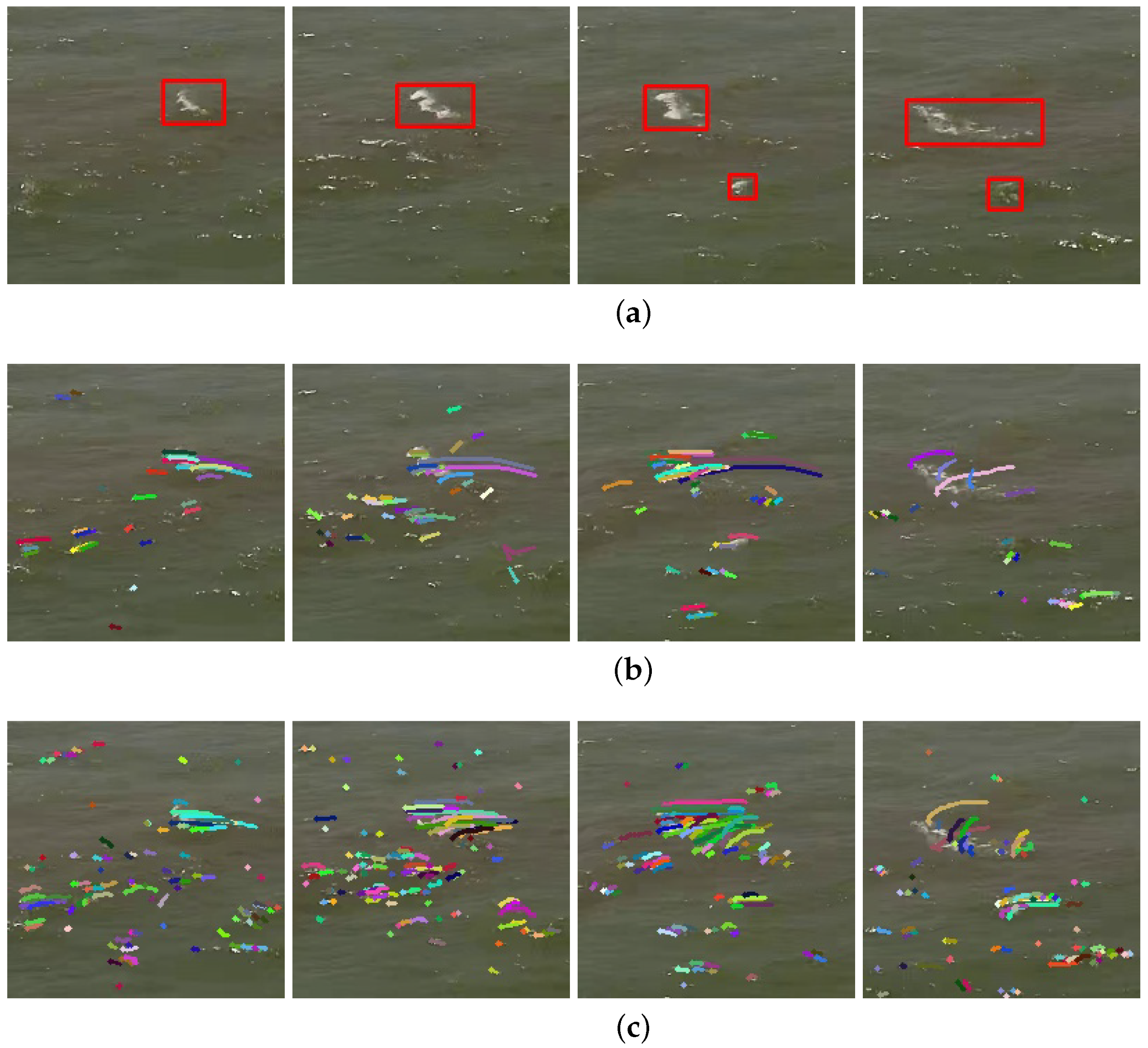
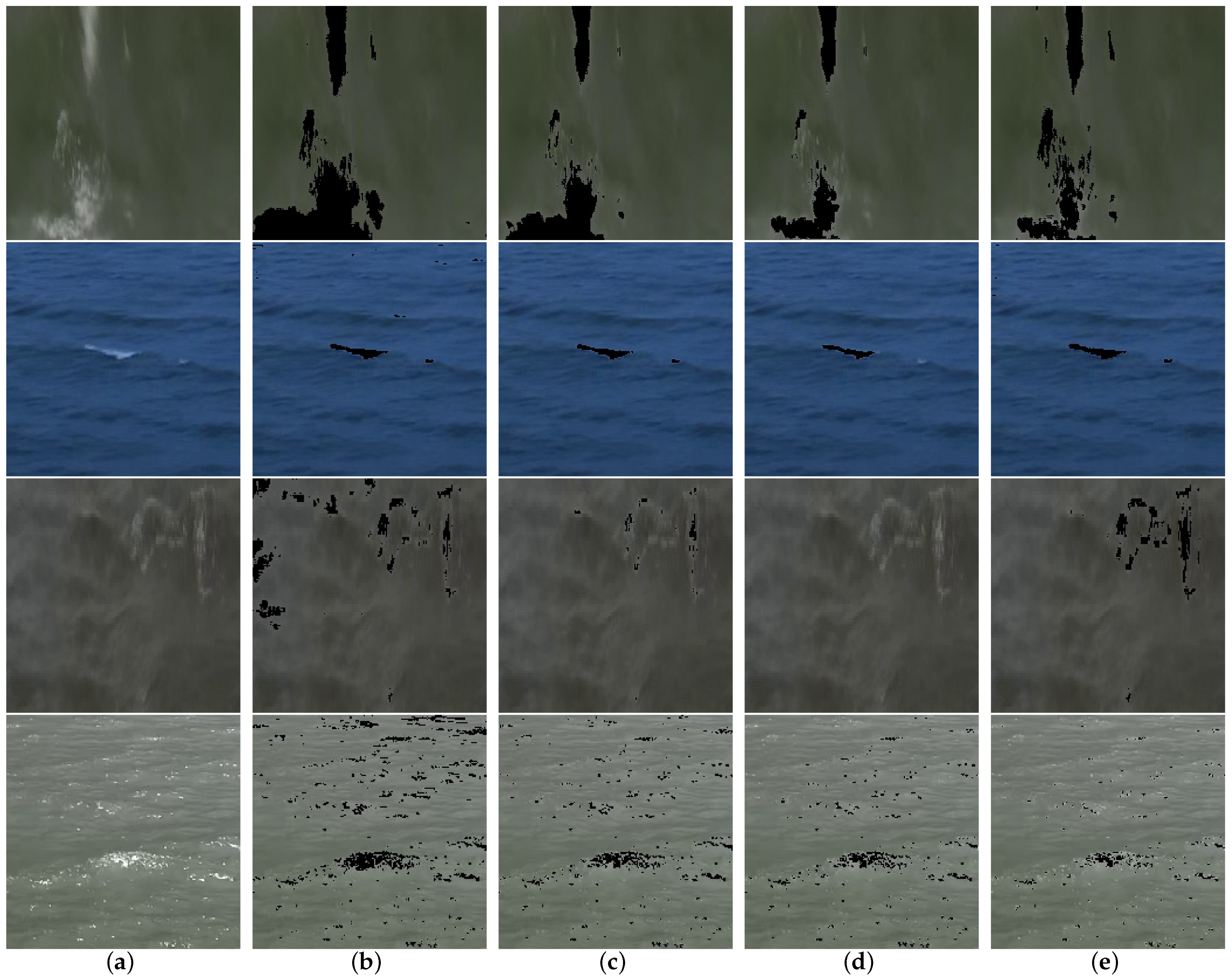
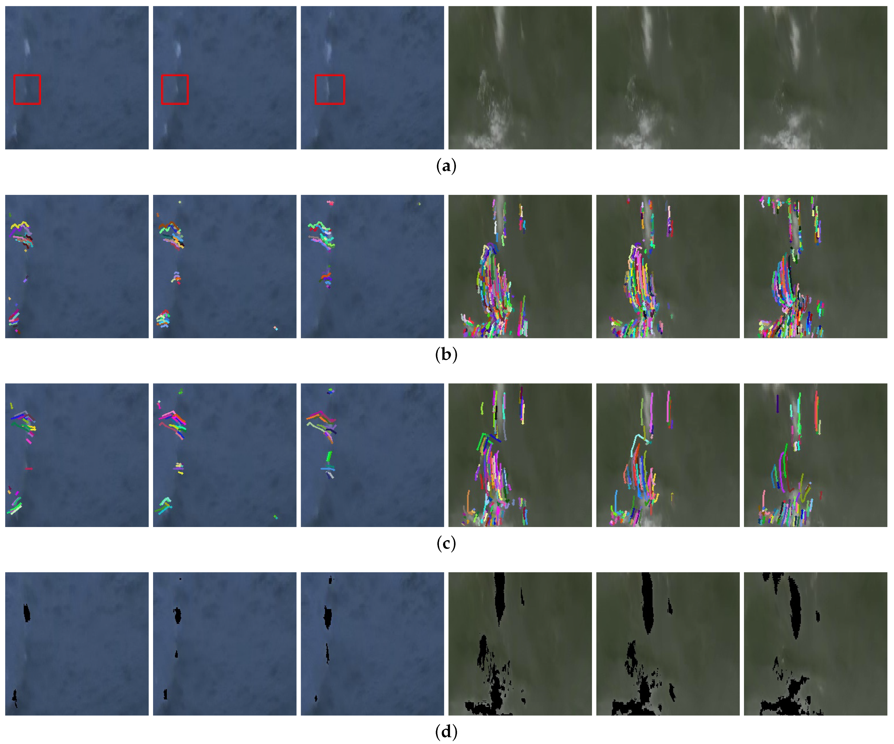
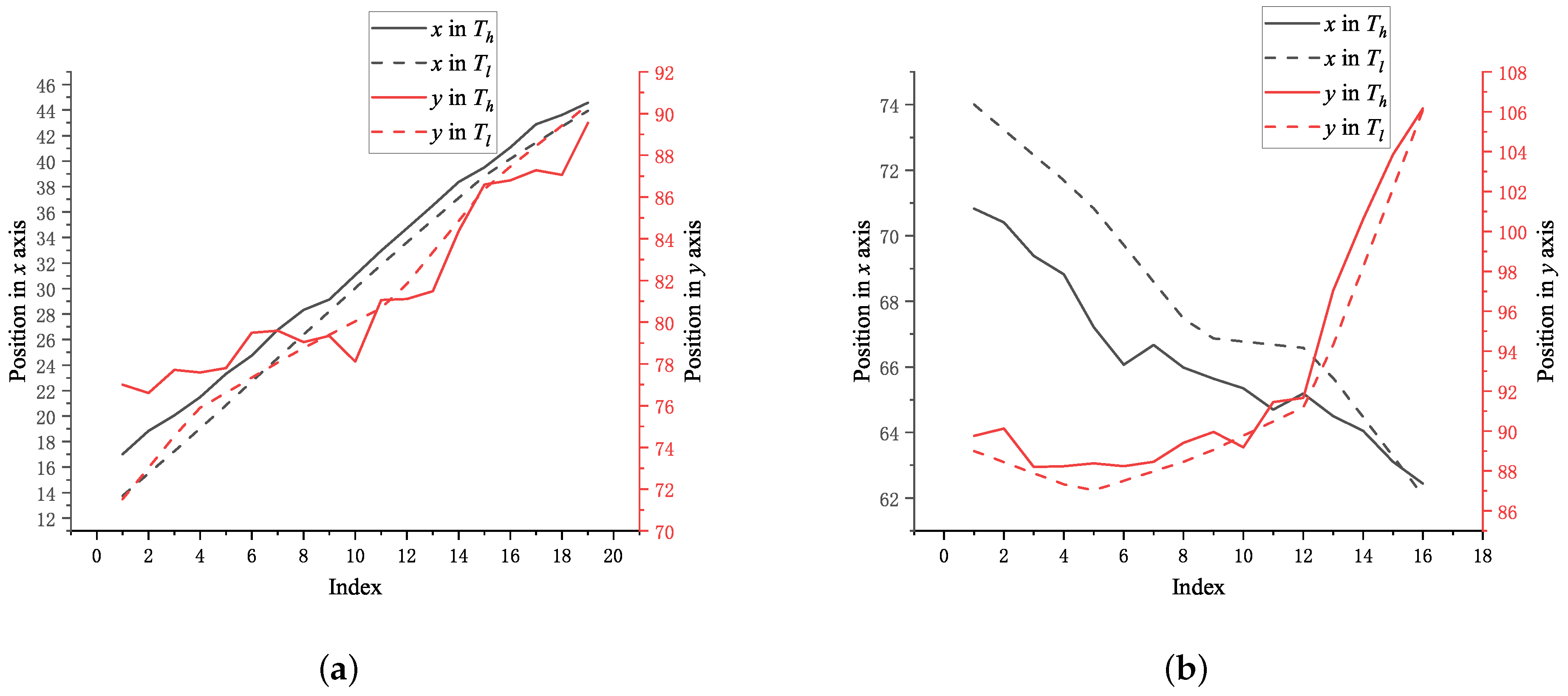
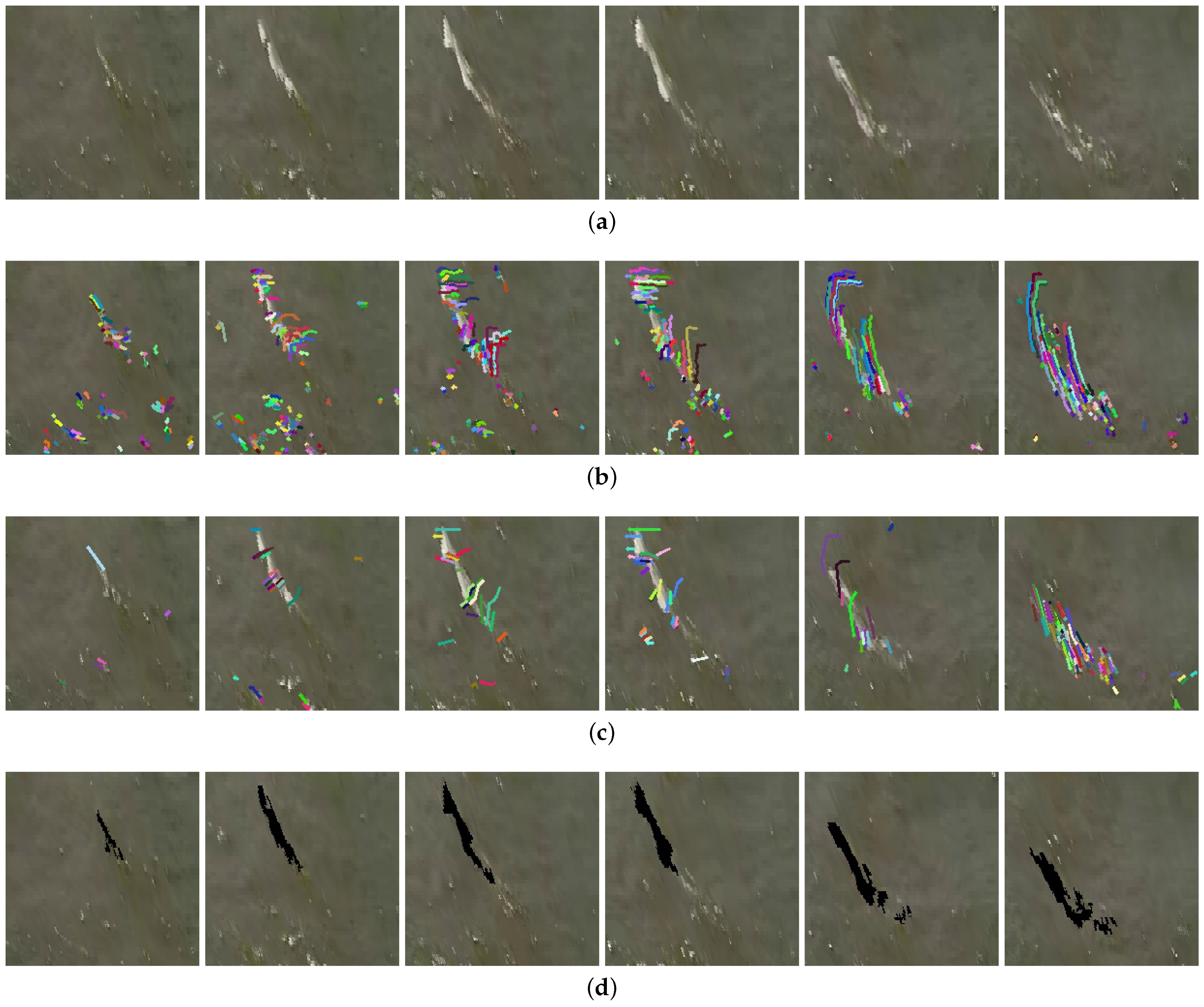
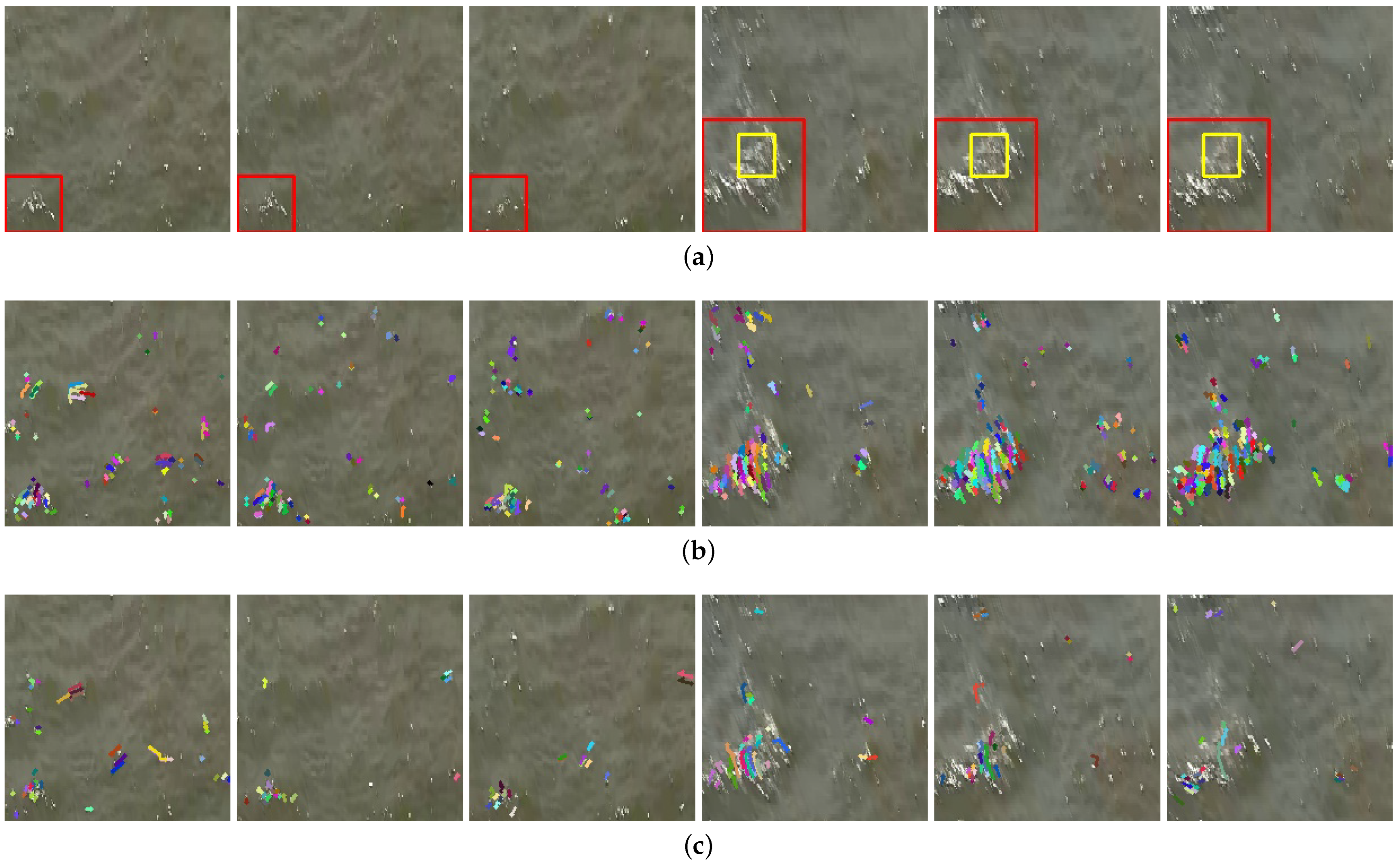
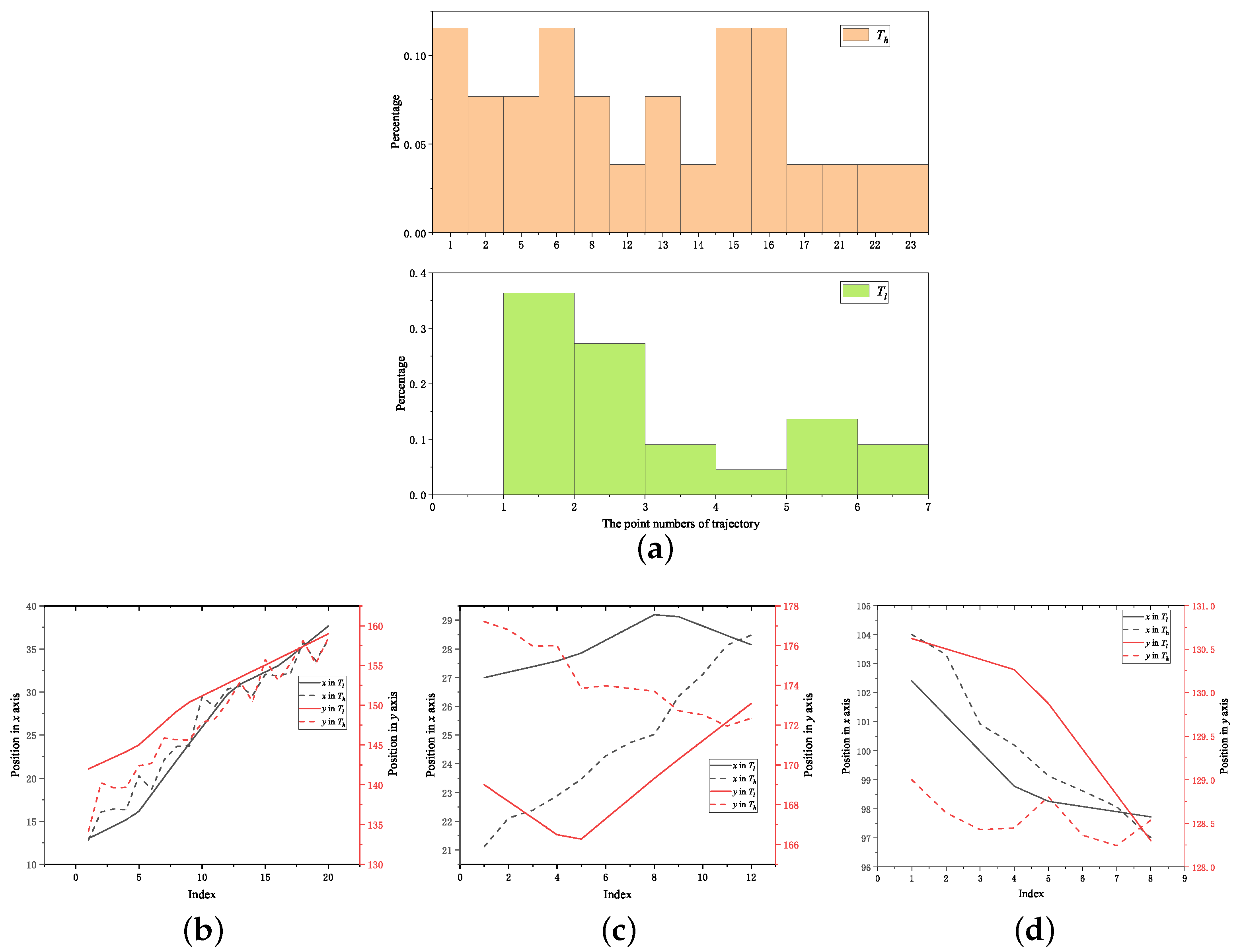
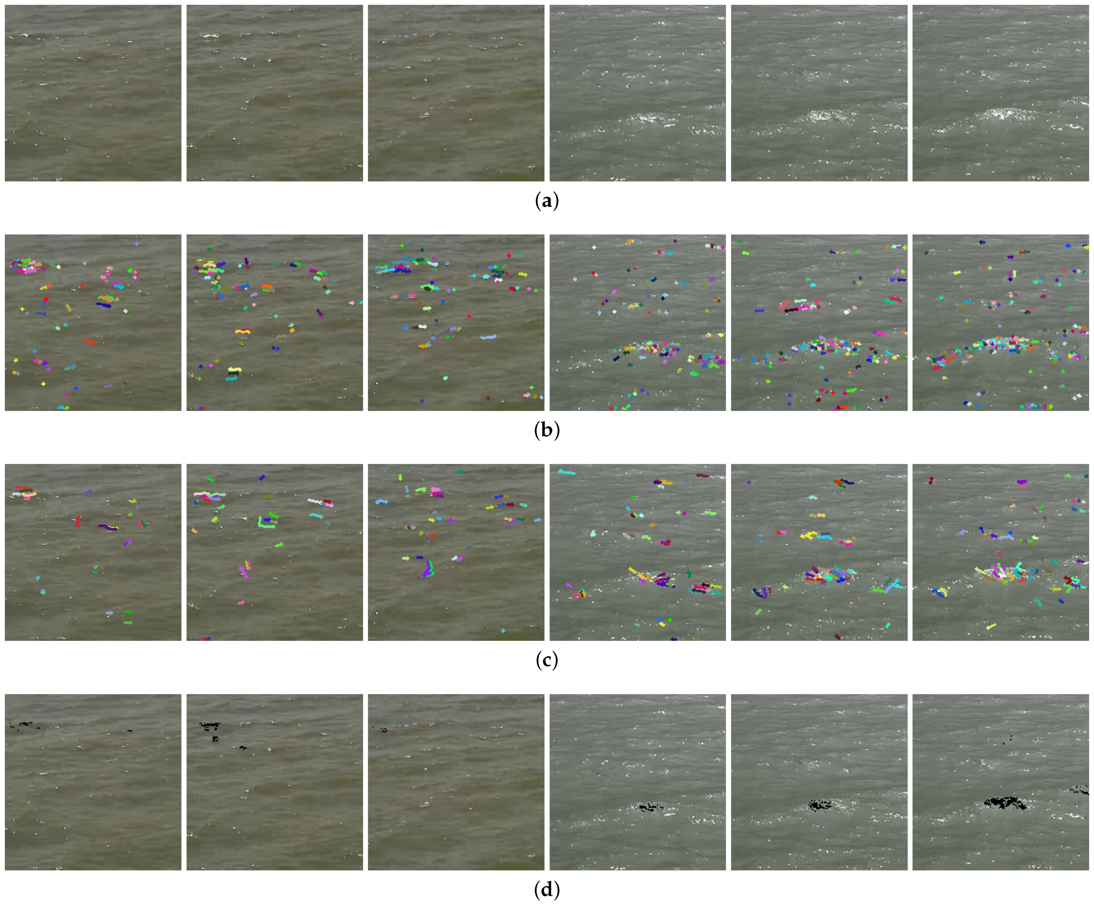
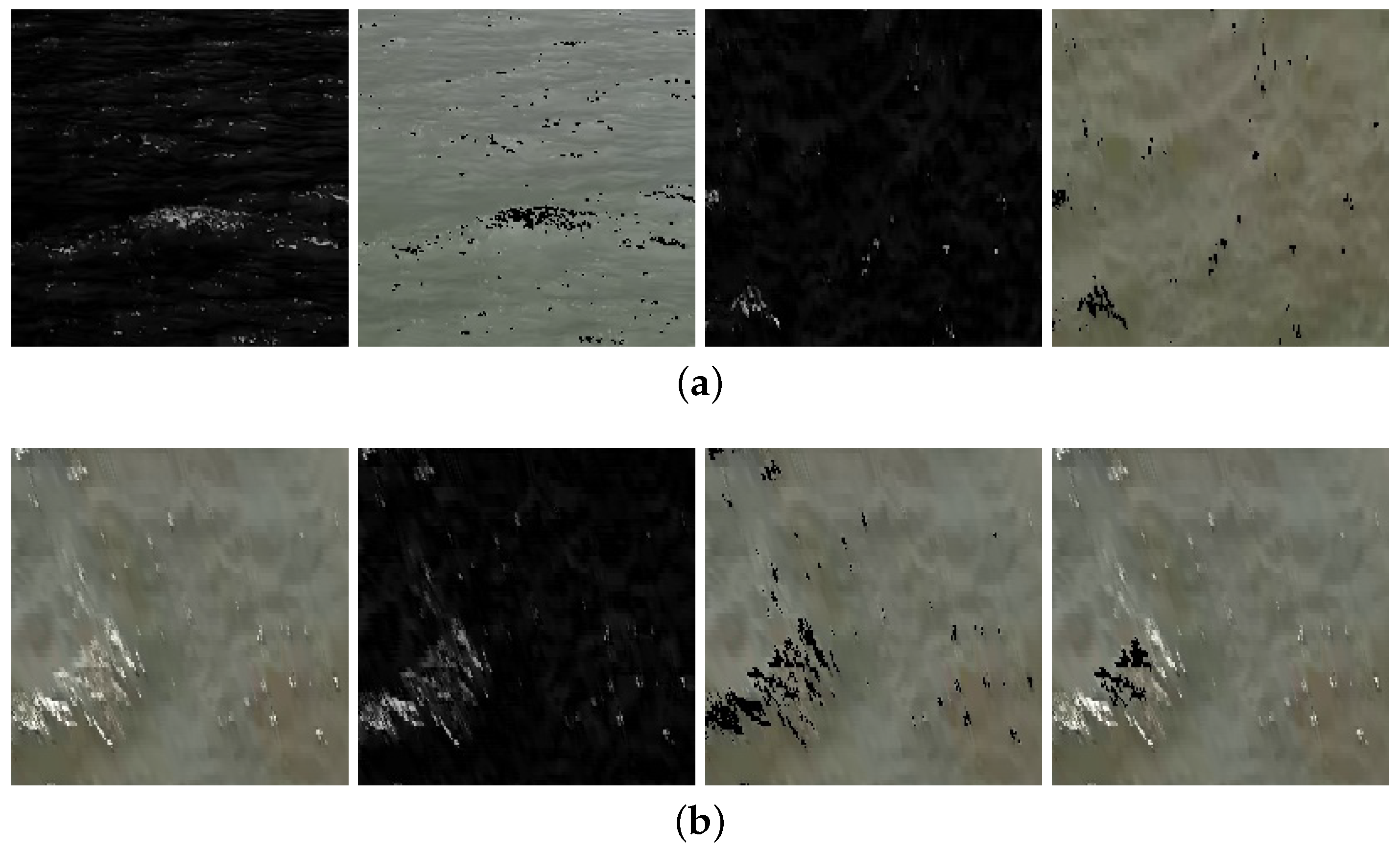
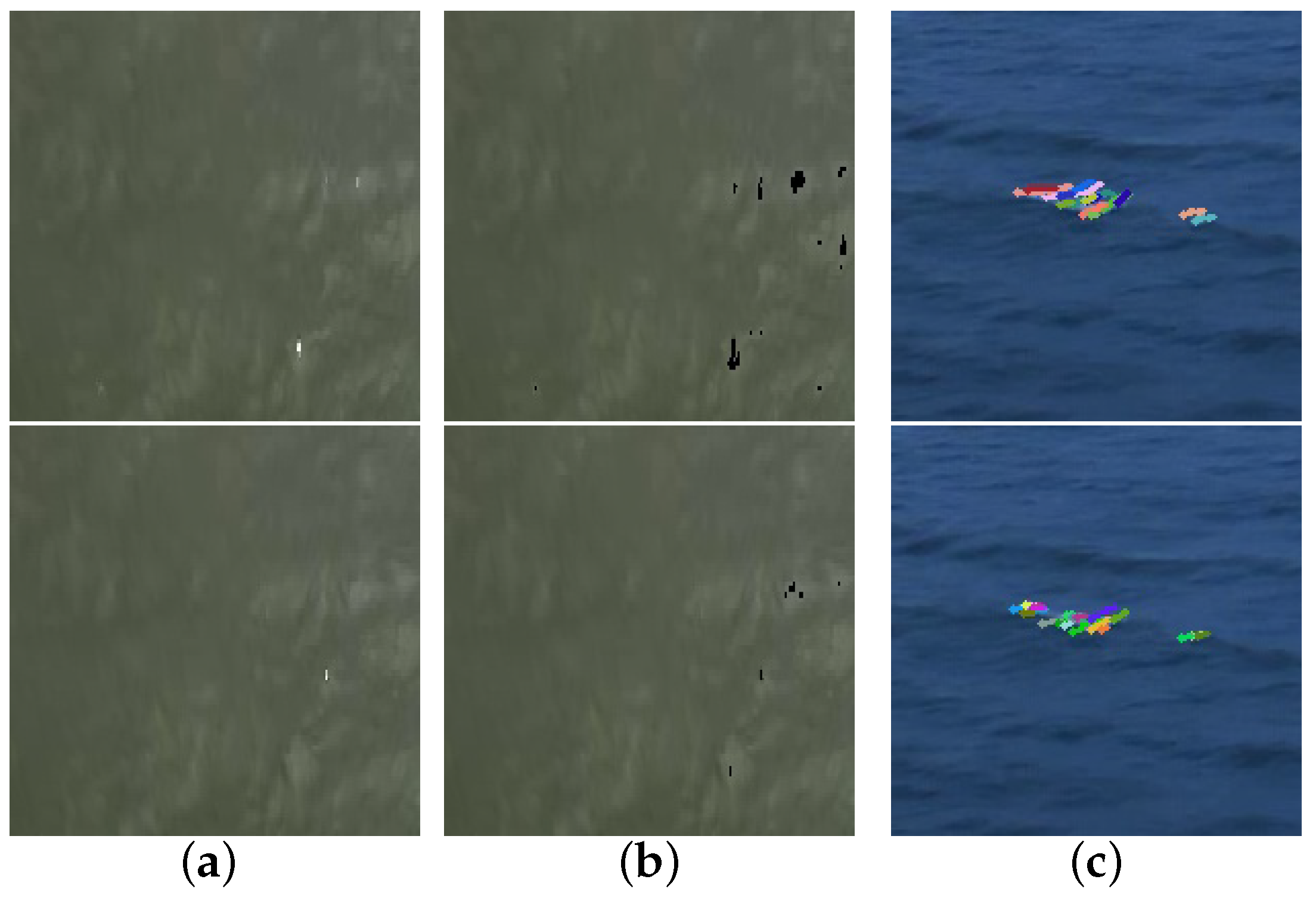
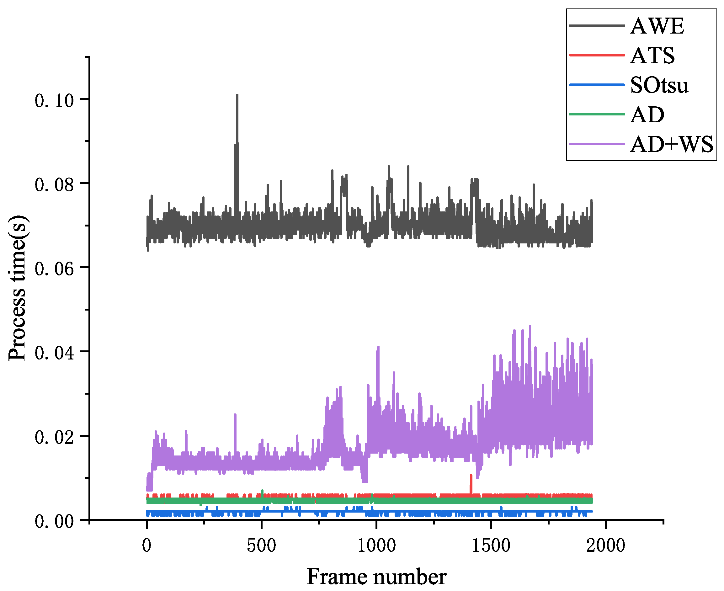
Table 1.
Comparison of W obtained by different methods; in each method column, the first data are W, and the second data are the relative error (RE) between the ground truth and obtained W. Text is bolded to indicate that the method performs best in this case.
Table 1.
Comparison of W obtained by different methods; in each method column, the first data are W, and the second data are the relative error (RE) between the ground truth and obtained W. Text is bolded to indicate that the method performs best in this case.
| Number | Ground (%) | AWE/RE (%) | ATS/RE (%) | SOtsu/RE (%) | Our’s/RE (%) |
|---|---|---|---|---|---|
| 1 | 7.70 | 13.35/73.38 | 7.84/1.82 | 5.38/30.13 | 7.46/3.12 |
| 2 | 0.61 | 0.73/19.67 | 0.55/9.84 | 0.45/26.23 | 0.67/9.84 |
| 3 | 2.86 | 3.65/27.62 | 0.50/17.48 | 0.00/100.00 | 2.38/16.78 |
| 4 | 0.00 | 5.42/- | 2.95/- | 2.25/- | 1.27/- |
Table 2.
The longest trajectory lengths from whitecaps and sun glints at different sampling rates. represents the maximum trajectory length from whitecaps, and represents the maximum trajectory length from sun glints. The data format is / , which represents the trajectory lengths at high and low sampling rates, respectively.
| Image Number | 1 | 2 | 3 | 4 | 5 | 6 |
|---|---|---|---|---|---|---|
| 4/2 | 13/3 | 21/4 | 25/6 | 25/4 | 25/5 | |
| 14/2 | 7/3 | 10/2 | 17/3 | 5/2 | 4/2 |
Table 3.
Comparison of detection results of different methods under light pollution of a specific shape.
Table 3.
Comparison of detection results of different methods under light pollution of a specific shape.
| Case | Ground (%) | ATS (%) | AD (%) | SOF (%) | OFTC (%) |
|---|---|---|---|---|---|
| 0.00 | 0.89 | 0.86 | 0.48 | 0.00 | |
| 0.31 | 3.50 | 3.21 | 0.80 | 0.23 | |
| 0.00 | 0.66 | 0.85 | 0.54 | 0.00 | |
| 0.00 | 2.55 | 0.54 | 0.32 | 0.00 |
Publisher’s Note: MDPI stays neutral with regard to jurisdictional claims in published maps and institutional affiliations. |
© 2022 by the authors. Licensee MDPI, Basel, Switzerland. This article is an open access article distributed under the terms and conditions of the Creative Commons Attribution (CC BY) license (https://creativecommons.org/licenses/by/4.0/).
Share and Cite
MDPI and ACS Style
Hu, X.; Yu, Q.; Meng, A.; He, C.; Chi, S.; Li, M. Using Optical Flow Trajectories to Detect Whitecaps in Light-Polluted Videos. Remote Sens. 2022, 14, 5691. https://doi.org/10.3390/rs14225691
AMA Style
Hu X, Yu Q, Meng A, He C, Chi S, Li M. Using Optical Flow Trajectories to Detect Whitecaps in Light-Polluted Videos. Remote Sensing. 2022; 14(22):5691. https://doi.org/10.3390/rs14225691
Chicago/Turabian StyleHu, Xinyao, Qianxiang Yu, Ankang Meng, Chenglong He, Shukai Chi, and Ming Li. 2022. "Using Optical Flow Trajectories to Detect Whitecaps in Light-Polluted Videos" Remote Sensing 14, no. 22: 5691. https://doi.org/10.3390/rs14225691
Note that from the first issue of 2016, this journal uses article numbers instead of page numbers. See further details here.