Remote Sensing Scene Graph and Knowledge Graph Matching with Parallel Walking Algorithm

Abstract

In deep neural network model training and prediction, due to the limitation of GPU memory and computing resources, massive image data must be cropped into limited-sized samples. Moreover, in order to improve the generalization ability of the model, the samples need to be randomly distributed in the experimental area. Thus, the background information is often incomplete or even missing. On this condition, a knowledge graph must be applied to the semantic segmentation of remote sensing. However, although a single sample contains only a limited number of geographic categories, the combinations of geographic objects are diverse and complex in different samples. Additionally, the involved categories of geographic objects often span different classification system branches. Therefore, existing studies often directly regard all the categories involved in the knowledge graph as candidates for specific sample segmentation, which leads to high computation cost and low efficiency. To address the above problems, a parallel walking algorithm based on cross modality information is proposed for the scene graph—knowledge graph matching (PWGM). The algorithm uses a graph neural network to map the visual features of the scene graph into the semantic space of the knowledge graph through anchors and designs a parallel walking algorithm of the knowledge graph that takes into account the visual features of complex scenes. Based on the algorithm, we propose a semantic segmentation model for remote sensing. The experiments demonstrate that our model improves the overall accuracy by 3.7% compared with KGGAT (which is a semantic segmentation model using a knowledge graph and graph attention network (GAT)), by 5.1% compared with GAT and by 13.3% compared with U-Net. Our study not only effectively improves the recognition accuracy and efficiency of remote sensing objects, but also offers useful exploration for the development of deep learning from a data-driven to a data-knowledge dual drive.

1. Introduction

In the application of recognizing complex geographical scenes, graph neural networks (GNNs) can consider semantic and spatial relationships between recognition units generated from geographical objects. Therefore, object-based GNNs can represent and process the graph structure information of remote sensing objects to accomplish the segmentation of remote sensing scenes more efficiently than a pixel-based model [1,2,3]. Due to the limitation of GPU memory and computing resources, massive image data must be cropped into samples with limited size for model training [4]. Additionally, to ensure the generalization ability of the model, the samples’ coverage area is limited, and their locations are randomly distributed, so the background information is often incomplete or even missing. Therefore, it is necessary for GNNs to use geographic knowledge graphs to recognize complex geographical scenes [1,2]. In this way, GNNs can use more universal geographic background knowledge. The geographic categories involved in the knowledge graph are comprehensive and systematic.

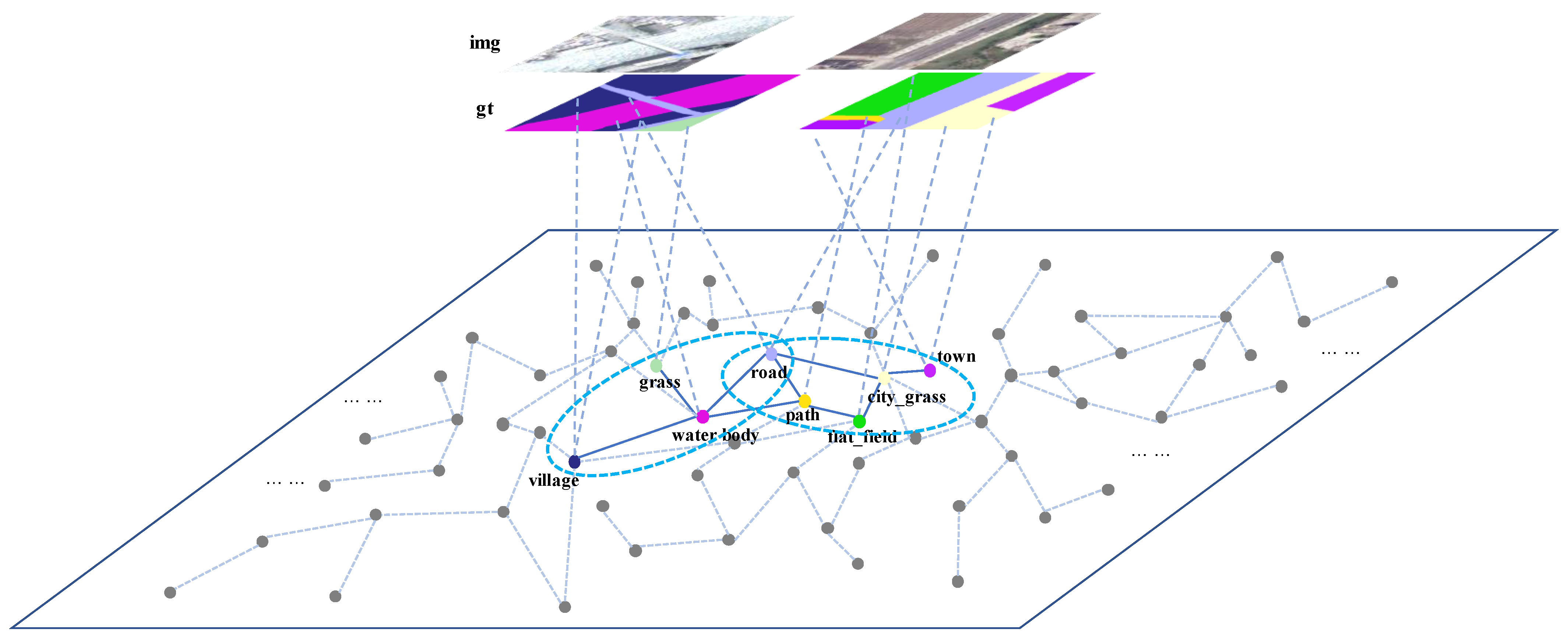
However, when the knowledge graph is applied to the recognition of complex geographical scenes, the categories are limited in a single sample. But they are complex in different samples. Without differential treatment, the model can only use the complete category set as the output, which is inefficient and a combinatorial explosion, as shown in Figure 1.

To solve the above problems, a parallel walking algorithm (PWGM) based on cross modal information is proposed. Our PWGM achieves graph matching between generalized knowledge graphs in knowledge modality and specific remote sensing image scene graphs in visual modality. Therefore, it integrates geographical knowledge into complex geographic scenes and efficiently accomplishes semantic segmentation tasks of remote sensing images. On this basis, we propose a semantic segmentation model for remote sensing based on PWGM.

The experimental results show that the model proposed in this paper can effectively improve the recognition performance of remote sensing objects. To summarize, the main contributions are as follows: In Section 2.2, a Scene Graph Optimization Module based on cosine similarity graph pooling is designed to construct and optimize the sample scene graph. The algorithm clusters remote sensing objects whose feature similarity can meet the threshold into the “superpixel group”, whose feature similarity can meet the threshold to merge the redundant nodes of the scene graph to achieve the graph’s optimization.

In Section 2.3.2, a parallel walking algorithm is designed for matching scene graphs and knowledge graphs. Compared with all categories of the knowledge graph as candidates, the number of categories involved in the knowledge subgraph provided by the walking algorithm is less and the matching with specific samples is more precise. Taking this as the basis for segmentation, it can reduce the network parameters and improve the efficiency by freezing those categories outside the knowledge subgraph; moreover, the phenomenon of “different objects with the same spectrum” is avoided to a certain extent.

In Section 2.4, a Knowledge Subgraph-Based Superpixel Group Classification Module is designed. The “superpixel group” obtained from the proposed cosine similarity-based graph pooling algorithm of remote sensing objects is used as the segmentation unit to improve the efficiency of segmentation.

1.1. Graph Neural Networks and Remote Sensing Semantic Segmentation

Semantic segmentation has always been a crucial research component in the field of remote sensing [5,6,7,8].

At present, GNNs in deep learning are effective for the semantic segmentation of remote sensing images [9,10,11]. Zhang et al. [12] used pixels in small blocks to construct an adjacency matrix. It cooperated with a graph convolutional network (GCN) [13] to make full use of local spatial information to improve the classification efficiency on hyperspectral classification tasks. Yang et al. [14] proposed a new graph construction method when performing visual recognition tasks, extracting useful information from RGB images. The method used GCN to incorporate this information into graph data, greatly improving graph classification accuracy. Ma et al. [15] used GCN to fuse superpixel block information to improve the classification performance on SAR image segmentation tasks after superpixel segmentation.

When applying remote sensing images to identify complex geographic scenes, samples are limited and randomly distributed, and consequently, background information is usually missing. This phenomenon leads to the limitation of the generalization ability of GCN, and its difficulty in recognizing complex geographic scenes. Wu et al. [16] designed a multi-scale GCN to extract features from remote sensing objects. This method updates node information separately and uses fusion strategies to integrate multiple scales. The ground object information is fused for classification, which uses rich scale information to account for the imbalance of sample information. Cui et al. [2] proposed a method to weight the importance of relationships between geographical objects through prior knowledge. This method accomplished the information aggregation by applying external knowledge to guide and control the characteristics of object nodes. It provides more explicability for node classification. Ding et al. [17] learned multi-scale features from local region graphs based on GraphSAGE and used a context-aware mechanism to characterize the importance between spatially adjacent regions. By focusing on important spatial objects, this method automatically learns deep contextual and global information for graph data.

In current research, the construction of scene graph of remote sensing image sample is complex. In addition, the background information is missing due to random clipping. This phenomenon affects the performance of the classification of remote sensing objects by GNN. However, our model provides background information based on the knowledge graph to improve the model performance.

1.2. Geographical Knowledge Graph

Chen et al. [18] proposed the concept of the geographical graph for the first time, and then many other researchers have conducted studies. These studies include the vegetation graph, hydrological graph, land cover graph, etc. These graphs are variants of the geographic graph [19,20,21,22]. Inspired by other areas of the scientific community, Xu et al. [23] proposed a new concept of the geoscience knowledge graph, which represents geography’s proprietary knowledge by using graphical elements.

In the application of geography, knowledge graphs use geographic concepts or phenomena (nodes) and their semantic or symbiotic relationships (edges) to form a graph structure. It is a general method for storing and sharing geographic prior knowledge. However, there some shortcomings remain. Since the structure of the knowledge (graph) is relatively fixed, at the beginning of the prediction process of GNN, the geographical object label cannot be determined. Therefore, it cannot be directly located to the knowledge graph, rendering it necessary to match the scene graph and knowledge graph according to the characteristics and spatial relationship of the nodes in the training process, and obtaining the ability of knowledge embedding [24,25,26].

The semantics and categories involved in geographic knowledge graphs greatly exceed the geographic scenes contained in specific samples. Therefore, geographic knowledge cannot be used efficiently or correctly to assist the semantic segmentation of remote sensing images. It is crucial to pool complex remote sensing image scene graphs at the same time. Under these circumstances, our model designs an accurate scene graph—knowledge graph matching mechanism to apply geographic knowledge to remote sensing image semantic segmentation, which improves the model efficiency.

1.3. Graph Pooling

With the development of GNN, graph pooling has attracted much attention. A pooling layer is designed to reduce the model parameters by reducing the scale of the graph structure and avoid over-fitting. It also plays an important role in Euclidean structure data, which can reduce the size of the feature map, enlarge the receptive field and enhance the generalization ability of the network.

Sun et al. [27] divided graph pooling methods into cluster pooling and top-k selection pooling.

The cluster pooling method clusters graph nodes according to a certain relationship between nodes. This pooling method indirectly utilizes graph structure and graph node characteristics. The number of clusters must be set in advance to guide the clustering process, which incurs massive computing costs. Sun et al. [28] mentioned that most graph pooling methods only consider node feature and graph structure without the semantic information of substructures. To solve this problem, they proposed a subgraph level clustering pooling method that learned a rich subgraph feature. Ying et al. [29] proposed DiffPool, a differentiable graph pooling method that uses graph convolution to learn an assignment matrix for nodes in each layer, mapping the nodes to different categories.

The top-k selection pooling method calculates a score for each node. The score represents the importance of nodes and help to select top k important nodes. By removing the remaining nodes from the graph structure, this method avoids the large computational cost introduced in clustering pooling. Such pooling methods as SortPooling [29] utilize the structural importance scores of nodes in the graph to rank the nodes and select the top k nodes for the graph pooling operation. However, the pooling method needs to set hyper-parameter k in advance. It must be tested continuously during the experiment, which also leads to the weak generalization ability of the model. In order to better highlight the role of graph pooling, SAGPool [30] proposed a self-attention graph pooling method that uses graph convolution to take node feature and graph structure into account. The results show that the self-attention graph pooling method reduces the size of the graph structure and improves model training efficiency. Li et al. [31] considered both graph structure and feature information. They aggregated node feature information before discarding unimportant nodes, so that the selected node contains information from neighbor nodes. In this way, the model can make full use of the unselected node feature. Other graph pooling methods [32,33,34,35,36] are also designed and show good performance.

Compared with the above graph pooling methods, our method uses cosine similarity to filter important nodes in the knowledge graph, which is more flexible and efficient.

1.4. Graph Walking Algorithm

A graph walking algorithm generally walks through the graph in a certain way to obtain multiple sequences and uses them to learn the graph representation. The low dimensional representation of nodes can be learned through graph representation and the relationship between nodes (node embedding). Then, the algorithm uses node embedding for downstream tasks. Node2Vec [37] selects nodes by calculating the transition probability of neighbor nodes and implements graph walking. Nasiri E et al. [38] improved Node2Vec for node embedding generation on the prediction of interactions in protein. C. Shi et al. [39] improved Node2Vec in a heterogeneous information network (HIN) and proposed a new method based on heterogeneous network embedding. Network representation learning (NRL) [40] improves the traditional social network, knowledge edge graph and graph mining of complex biomedical and physical information networks.

In addition to node embedding tasks, a graph walking algorithm can also be utilized to search specific subgraphs. Metapath2vec [41] can be used for node classification, clustering and subgraph similarity search.

1.5. Geographical Knowledge Graph and Remote Sensing Image Scene Graph Matching

In computer vision, scene–knowledge graph matching mainly adopts three types of methods. First, each node in the scene graph traverses all category combinations of the knowledge graph for knowledge embedding. However, the search space of this method is too large, and the calculation cost is too high [42,43]. Second, special networks are designed towards knowledge in nodes for knowledge embedding. However, this method increases the parameters of the network, which affects the convergence speed of the model, and the conclusions are unexplainable. Third, calculating the node similarity in the scene graph and knowledge graph achieves the knowledge graph embedding [44,45]. However, the visual feature and the word embedding feature belong to different feature modalities. The gap is hard to ignore, and the similarity cannot be directly calculated.

Some studies apply prior knowledge to remote sensing image analysis. Sharifzadeh et al. [46] used biLSTM to model category dependencies for the multilabel classification of aerial images. Hua et al. [47] incorporated symbiotic dependencies into the Markov random field model to achieve remote sensing image classification. However, there is little research on applying scene–knowledge graph matching into remote sensing image analysis.

Object-based remote sensing image analysis methods can carry richer semantic information. GNNs structure the representation in non-Euclidean space. This model has a stronger and more effective spatial information expression ability [48]. Geographical knowledge graph can store and share knowledge, while the scene segmentation of remote sensing images needs to embed geographic prior knowledge through graph matching. However, there are few studies on the scene segmentation of remote sensing images based on geographical objects, GNN and knowledge graphs.

The current matching algorithm has a wide search range, high computational cost, and low matching accuracy, which requires further exploration. Thus, we design a parallel walking algorithm to achieve scene graph—knowledge graph matching. By reducing redundant nodes in the knowledge graph, it improves the model accuracy and efficiency.

The research field of related work is shown in

Table 1. Introduction of references.

Research Field	References
Remote sensing semantic segmentation	[1,2,3,4,5,6,7,8,11,15,47]
Graph neural network	[9,10,11,12,14,16,43,48,49]
Graph construction method	[13,24,46]
Research on geographical knowledge graph	[17,18,19,20,21,22,23,25]
Graph pooling method	[26,27,28,29,30,31,32,33,34,35]
Scene graph–knowledge graph matching method	[36,42,43,44,45]
Graph walking method	[37,38,39,40,41]
Graph matching method	[43]

. The related work involved mainly contains the graph method and semantic segmentation in remote sensing. Our aim is to propose a semantic segmentation method based on a parallel walking algorithm using the scene graph—knowledge graph matching method.

Under these circumstances, an accurate knowledge graph and scene graph matching mechanism is designed to apply geographic knowledge to remote sensing image semantic segmentation.

The notations used in this article are shown in

Table 2. Table of notations.

Symbol	Meaning
$F_V$	the visual feature of nodes in the scene graph
$GAP$	global average pooling
$CNN$	convolutional neural network model
x	image samples
$objMask$	the superpixel mask
$G_{sg}$	the sample scene graph structure
$V_{sg}$	the node set of the scene graph
$E_{sg}$	the edge set of the scene graph
$v_i$	the visual feature cosine similarity
$e_{ij}$	the edge between nodes i and j
$Simalarity\left(F_{V_i},F_{V_j}\right)$	$\mathrm{the}\cos \mathrm{ine}\mathrm{similarity}\mathrm{between}\mathrm{node}\mathrm{feature}\mathrm{vectors}{F}_{V_i}$$\mathrm{and}{F}_{V_j}$
$d$	the feature dimension of the vector
$gMask$	group mask matrix
$cosSim$	cosine similarity matrix
$threshold$	clustering threshold
$F_{inner}$	the node features updated from neighbor nodes within the group
$\sigma$	activation function
$W$	learnable matrix
$gAs{s}_{\left(\tau ,i\right)}$	the assignment weight of node i which belongs to the superpixel group $\tau$
$F_{hid\_group}$	the superpixel group feature matrix
$G_{kg}$	the structure of knowledge graphs for remote sensing semantic segmentation
$V_{kg}$	the node set of the knowledge graph
$E_{kg}$	the edge set of the knowledge graph
$c{o}_{\alpha \beta }$	the category cooccurrence probability between nodes $\alpha$ and $\beta$
$n_{\alpha \beta }$	the number of samples that include categories $\alpha$ and $\beta$
$n_{\alpha }$	the number of samples that include category α
$Scor{e}_{\left(c\right)}$	the classification score of category $c$
$c{o}_{\left(bc\right)}$	the cooccurrence probability of categories b and c
$p_{\left(c\right)}$	the next node score of the multilabel classification
$\lambda ,\phi ,\mu$	hyperparameters
$F_{mixfg}$	the final mixed feature
$Att$	attention function
$F_{group }$	the final superpixel group feature
$F_{U }$	the word embedding features of nodes in the knowledge graph
$GAT$	graph attention network
$Output$	the result of classification
$softmax$	normalization function
${\mathcal{L}}_{semantic}$	the cross-entropy loss function of superpixel groups semantic classification
$y$	the label of the superpixel groups semantic classification
$\widehat{y_i}$	the prediction result of the superpixel groups semantic classification

and the subsequent chapters of this paper are as follows: Chapter 2 focuses on our proposed PWGM, Chapter 3 focuses on experiments and Chapter 4 analyses the results of the experiments in detail and explains the mechanism. In Chapter 5, future work is proposed.

2. Materials and Methods

This chapter introduces the semantic segmentation model of remote sensing images based on a parallel walking algorithm (PWGM). First, it comprehensively summarizes the structure of the model, and then focuses on the innovative work of this paper: a clustering graph pooling algorithm based on cosine similarity and a scene graph–knowledge graph matching algorithm based on the parallel walk algorithm.

2.1. Network Structure

This section mainly introduces the structure of our semantic segmentation model based on PWGM, which consists of four parts.

• Superpixel Visual Feature Extraction Module;
• Scene Graph Optimization Module based on cosine similarity graph pooling;
• Scene Graph–Knowledge Graph Matching Module based on parallel walking algorithm;
• Knowledge Subgraph-Based Cross Modality Superpixel Group Classification Module.

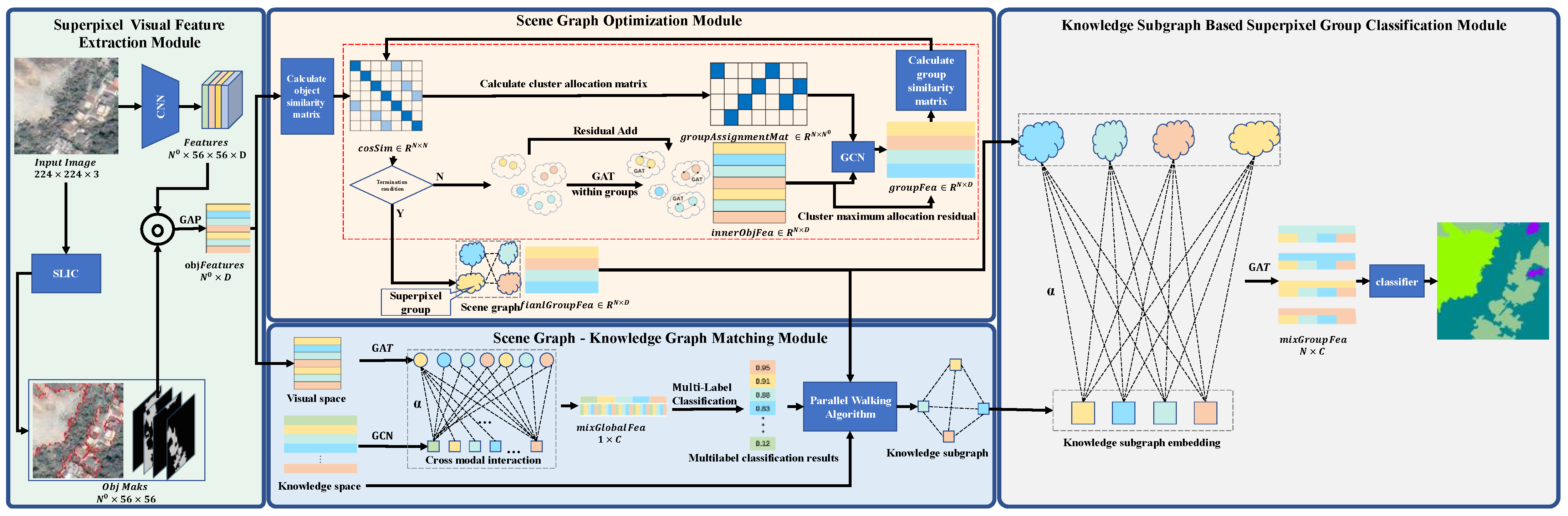
The modules are shown in Figure 2 below.

• Superpixel Visual Feature Extraction Module

First, we extract the global visual features of the image samples by a pre-trained CNN model that consists of two consecutive 3 × 3 convolutions and 2 × 2 max pooling. Then, simple linear iterative clustering (SLIC) is used to obtain the superpixel mask ($N^0\times W/4\times H/4$), where $N$ denotes the number of superpixels. Finally, the visual feature of the superpixel is obtained from global average pooling (GAP), and the input of GAP is obtained from the matrix Hadamard product between the sample global visual feature and the superpixel mask.

$$F_V=GAP\left(\left(CNN\left(x\right)\circ objMask\right)\right)$$

(1)

In Formula (1), $F_V$ denotes the visual feature of the nodes in the scene graph, where $F_V\in R^{N^0\times D}$. $N^0$ represents the initial number of nodes in the scene graph corresponding to the number of superpixels, and $D$ denotes the feature dimension. $x$ denotes image samples, where $x\in R^{W\times H\times 3}$, $W$ and $H$ represent the width and height of the image. $objMask$ denotes the superpixel mask, where $objMask\in R^{W\times H\times N^0}$. $\prime \circ \prime$ denotes the Hadamard product.

2.

Scene Graph Optimization Module based on cosine similarity graph pooling

In this module, a scene graph pooling algorithm based on cosine similarity is designed to construct and optimize the scene graph. This module clusters superpixels by cosine similarity to filter the redundant nodes in the scene graph. The optimized sample scene graph can more precisely represent the category information of specific scene graphs and the correlation between them. This provides more accurate visual information for the Scene Graph—Knowledge Graph Matching Module. In this way, this module greatly improves the flexibility of the graph pooling algorithm compared with the traditional clustering graph pooling algorithm.

3.

Scene Graph—Knowledge Graph Matching Module based on parallel walking algorithm

This module, the crucial part of the model, matches the knowledge graph with the sample scene graph by a parallel walking algorithm. In the parallel walking algorithm, by regarding the score of the scene graph as a node feature of the generalized knowledge graph, we design a first-cross-modality method to merge the multilabel classification score of the scene graph into nodes in the knowledge graph. This enables the walking algorithm to consider the information of two modes simultaneously when walking in the knowledge graph, as well as the visual information of the scene graph and the cooccurrence probability between the nodes in the knowledge graph. The purpose of this module is to obtain the knowledge subgraph, which can precisely match the scene graph and greatly reduce the cardinal number of candidate categories sets.

4.

Knowledge Subgraph-Based Superpixel Group Classification Module

This module combines the visual features of superpixel groups with knowledge subgraph information. During the combination, we use graph attention networks (GATs) [49] to integrate information between the visual modality of the scene graph and the knowledge modality of the knowledge graph and achieve the classification of superpixel groups with knowledge subgraphs. In this second-cross-modality method, the node feature of the knowledge graph is the word-embedding feature of the corresponding category. The embedding information is integrated with the visual information of the superpixel groups. Notably, the classification process is based on a superpixel group rather than a superpixel. All the superpixels in the same group share the same label, which improves the model efficiency.

The following sections focus on the introduction of the Scene Graph Optimization Module and knowledge subgraph searching module-based parallel walking algorithm, which achieve scene graph pooling and match scene graphs with knowledge graphs, respectively.

2.2. Scene Graph Optimization Module Based on Cosine Similarity Graph Pooling

The superpixels obtained from the segmentation algorithm adopt the same scale, which leads to the problem of oversegmentation towards large-scale geographic objects. This results in redundant nodes and relationships in the scene graph and affects complex geographic scene recognition. Therefore, a cosine similarity-based graph pooling algorithm is designed to optimize it, as shown in Figure 3 below.

The input of the Scene Graph Optimization Module is the scene graph constructed by superpixels. The output is the scene graph optimized by superpixel groups and their edge features and cosine similarity. The red dashed box refers to the process of graph pooling.

We firstly construct a scene graph based on superpixels. In the scene graph, the nodes are superpixels, the features of the nodes are the visual features of superpixels, and the edges are the cosine similarity calculated by the visual features of superpixels. If the optimization condition is met, the clustering graph pooling process is performed; otherwise, the scene graph is output. As for the optimization condition, we calculate the cosine similarity between the nodes of the scene graph and judge its relationship with the empirical threshold. If the cosine similarity between two nodes is greater than the threshold, there are redundant nodes in the scene graph. On this condition, the scene graph needs to be optimized.

The graph pooling process performs node clustering based on the cosine similarity matrix, and the features of superpixels are obtained from aggregating the features of neighbor nodes within the same group by GAT. The group assignment matrix is calculated by the cosine similarity matrix of superpixels within the same group. We weight the updated feature of superpixels with the group assignment matrix to obtain the feature of the superpixel group.

The above pooling method avoids the loss of information caused by the pooling method based on node discarding. By iteratively updating the superpixel groups, the superpixels with similar features are clustered into the same groups, and as the basic unit of semantic segmentation, on the one hand, the geometric and visual features of each superpixel are retained. On the other hand, the scene graph is optimized, and redundant information is trimmed for subsequent segmentation. In this way, the efficiency and accuracy of classification can be improved.

2.2.1. Scene Graph Construction

The sample scene graph is constructed by the superpixels or superpixel groups. The following formula shows the sample scene graph structure $G_{sg}$:

$$G_{sg}=\left(V_{sg},E_{sg}\right)$$

(2)

In Formula (3), $V_{sg}$ denotes the node set of the scene graph, which is initially composed of $N_0$ superpixels. After the graph pooling process, it consists of $N$ superpixel groups. $E_{sg}$ denotes the edge set of the scene graph, which consists of cosine similarity calculated by the visual features of $V_{sg}$. The following formulas show the node set and the edge set of the scene graph.

$$V_{sg}=\left\{v_i,i\in \left\{1,\cdots , N\right\}\right\}$$

(3)

$$E_{sg}=\left\{e_{ij},i,j\in \left\{1,\cdots , N\right\}\right\}$$

(4)

In Formula (4), $e_{ij}$ denotes the edge between nodes i and j and is represented by the visual feature cosine similarity (Formula (5)) of $v_i$ and $v_j$.

Cosine similarity can express the abstract relationship of feature vectors, and its calculation formula is as follows:

$$Simalarity\left(F_{V_i},F_{V_j}\right)=\frac{{{\displaystyle \sum }}_{i=1}^d\left(F_{V_i}\times F_{V_j}\right)}{\sqrt{{{\displaystyle \sum }}_{i=1}^d{\left(F_{V_i}\right)}^2}\times \sqrt{{{\displaystyle \sum }}_{i=1}^d{\left(F_{V_j}\right)}^2}}$$

(5)

In Formula (5), $Simalarity\left(F_{V_i},F_{V_j}\right)$ denotes the cosine similarity between node feature vectors $F_{V_i}$ and $F_{V_j}$. $d$ represents the feature dimension of the vector.

Due to oversegmentation, scene graphs constructed by nodes probably retain redundant nodes and relationships, which affects complex geographic scene recognition. Therefore, a cosine similarity-based graph pooling algorithm is designed to optimize the scene graph.

2.2.2. Clustering Graph Pooling Based on Cosine Similarity

Clustering graph pooling can be divided into two processes: the judgement of scene graph optimization conditions and clustering graph pooling. The processes are described in detail below.

• Judgement of scene graph optimization condition

We use the cosine similarity matrix $cosSim$ of the nodes in the scene graph to define the condition. $cosSim$ is calculated by Formula (5). The clustering termination condition is whether the maximum of $cosSim$ is smaller than $threshold$. Clustering graph pooling is performed until the condition is met.

2.

Clustering graph pooling

First, group mask matrix $gMask$ is calculated based on $cosSim$ and the clustering threshold $threshold$, as shown in Formula (6).

$$gMas{k}_{\left(i,j\right)}=\{\begin{array}{c}1, cosSi{m}_{\left(i,j\right)}>threshold\\ 0, cosSi{m}_{\left(i,j\right)}<threshold\end{array}$$

(6)

$gMask$ is a group mask matrix used to define whether nodes $i$ and $j$ belong to the same group, where $gMask\in R^{N\times N}$ and $N$ correspond to the number of superpixel groups. $gMas{k}_{\left(i,j\right)}$ is the value of the group mask matrix. If $i$ and $j$ are clustered together, the value equals 1, else 0. $cosSim$ is the cosine similarity matrix, where $cosSim\in R^{N\times N}$. $cosSi{m}_{\left(i,j\right)}$ is the cosine similarity value of nodes $i$ and $j$. $threshold$ denotes the clustering threshold, which is a hyperparameter.

Second, the updated feature of node $F_{inner}$ is obtained by aggregating the feature of the neighbor node within the same group by GAT, where $F_{inner}\in R^{N\times D}$. The following formula shows the calculation expression of $H_{inner}$:

$$F_{inner}=\sigma \left(gMask\circ cosSim\times F_V\times W\right)+F_V$$

(7)

In Formula (7), $F_{inner}$ denotes the node features updated from neighbor nodes within the group and $F_{inner}\in R^{N\times D}$. σ denotes the activation function. $F_V$ denotes the visual feature of the nodes in the scene graph, where $F_V\in R^{N\times D}$. $W$ denotes the learnable matrix, where $W\in R^{D\times D}$. $\prime \circ \prime$ denotes the Hadamard product, and $\prime \times \prime$ denotes matrix multiplication.

Third, to calculate the weighted features of each node in the group as the overall visual features of the superpixel group, we firstly calculate the weight factor of each node in the group named group assignment matrix $gAss$.

$gAss$ represents the contribution of each node to the visual characteristics of the group. It is calculated based on the cosine similarity matrix of the nodes within the same superpixel group. The following formula shows the calculation of $gAss$:

$$gAs{s}_{\left(\tau ,i\right)}=\frac{{{\displaystyle \sum }}_{j=1,j\ne i}^{\psi }Simalarity\left(i,j\right)}{{{\displaystyle \sum }}_{k=1}^{\psi }{{\displaystyle \sum }}_{j=1,j\ne k}^{\psi }Simalarity\left(k,j\right)}$$

(8)

In Formula (8), $gAs{s}_{\left(\tau ,i\right)}$ denotes the assignment weight of node i, which belongs to superpixel group $\tau$, where $gAss\in R^{N\times N^0}$. $N$ represents the number of groups and $N^0$ represents the number of initial nodes in the scene graph. $\psi$ represents the node set in the superpixel group $\tau$, and $\prime \circ \prime$ denotes the Hadamard product. The numerator represents the sum of the cosine similarity between the node i and the other nodes in superpixel group $\tau$. The denominator represents the sum of the cosine similarity of the pairwise nodes in superpixel group $\tau$.

Finally, the superpixel group feature matrix $F_{hid\_group}$ is calculated based on $gAss$ and $F_{inner}$, where $F_{hid\_group}\in R^{N\times D}$, and D is the feature dimension.

$$F_{hid\_group}=\sigma \left(gAss\times F_{inner}\times W\right)+F_{V\left(\max \left(gAss\right)\right)}$$

(9)

In Formula (9), $F_{hid\_group}$ denotes the superpixel group feature matrix, where $F_{hid\_group}\in R^{N\times D}$. $\sigma$ denotes the activation function. $W$ denotes the learnable weight matrix, where $W\in R^{D\times D}$. To prevent the node features from being too smooth, we adopt the idea of residual, and superimpose the features of the nodes that contribute the most on the weighted features $F_{hid\_group}$. $F_{V\left(\max \left(gAss\right)\right)}$ is the node visual feature with the largest assigned weight within the group, where $F_{V\left(\max \left(gAss\right)\right)}\in R^{N\times D}$ and ‘×’ denotes matrix multiplication.

3.

Final optimized sample scene graph output

When the termination condition in scene graph optimization is met, the final optimized sample scene graph and its superpixel group feature $F_{group}$ are outputs, where $F_{group}\in R^{N\times D}$. This module optimizes the scene graph, and the number of nodes in the final optimized scene graph provides a termination condition for the parallel walking algorithm of scene graph–knowledge graph matching.

2.3. Scene Graph—Knowledge Graph Matching Module Based on Parallel Walking Algorithm

The knowledge graph is a universal knowledge system. It contains massive complex information. Conversely, a single sample often involves only a limited number of categories of knowledge graphs. When performing the semantic recognition of complex geographic scenes without matching scene graphs with knowledge graphs, we must traverse all categories as the classification candidate set of a single sample. This results in the “Combo Explosion” phenomenon. On the one hand, it increases the model parameters and computational cost. On the other hand, it reduces the accuracy of the model. Therefore, we propose a scene graph–knowledge graph matching mechanism based on parallel walking. The Scene Graph—Knowledge Graph Matching Module is shown in Figure 4.

Multilabel classification scores are obtained from a pretrained model, and the categories with the top two scores are used as the anchor points of parallel walking. Then, a parallel walking algorithm is designed to obtain a knowledge subgraph from the whole knowledge graph matched with the scene graph. The details are as follows.

2.3.1. Selecting Anchor Points of Parallel Walking Based on Multilabel Classification

To improve the efficiency and accuracy of graph matching, it is necessary to roughly determine the anchor point in the knowledge graph. The anchor point is the specific category in the knowledge graph matched with the most important object in the scene graph. For each scene graph, the anchor points are usually different and considered as the start of each walking process. Moreover, the anchor points of two walking-paths are selected based on multilabel classification scores.

The simple scene involved in this paper is a scene composed purely of rural or urban geographical objects. The complex scene is a combination of any two simple scenes mentioned above. In order to simplify the algorithm description, the complex scene in this paper is limited to the combinations of two simple scene, as shown in

Table 3. Sample statistics of complex scenes.

Scene Name	Number of Samples	Categories Involved	Definition of Scene	Type of Scene
Cultivated Scene	51	flat field (1), grass (3), terrace (9), strip field (10)	No village construction in cultivated scene	simple scene
Landslide scene	65	landslide (2), grass (3), water body (4), forest (12)	Surrounding environment of landslide	simple scene
Urban Scene	83	road (6), town (8), water body (4), city forest (13), city grass (11)	Surrounding environment of urban buildings	simple scene
Rural Scene	70	path (7), village (5), water body (4), forest (12), grass (3), flat field (1)	Surrounding environment of village construction	simple scene
Urban–rural scene	256	road (6), town (8), water body (4), city forest (13), city grass (11), path (7), village (5), forest (12), grass (3), flat field (1)	Urban rural fringe	complex scene
Landslide-influenced scenes	210	path (7), village (5), water body (4), forest (12), grass (3), flat field (1), landslide (2), road (6), town (8)	Surrounding environment of affected by landslides	complex scene
…	…	…	…	…

.

To better adapt to the different situations of simple and complex scenes, the following anchor selection strategies are formulated.

In a simple scene graph, the two categories with the highest score are treated as the anchor points. There are limited differences between two walking paths. In a complex scene graph, it consists of multiple simple scenes. In general, the most important categories often belong to different simple scenes and act as two-way anchor points. Otherwise, the second anchor point is reselected in a sequence according to the score until the two anchor points do not belong to the same scene.

The multilabel classification score $P$ is obtained by a remote sensing image fed into a pretrained multilabel classification network, where $P\in R^{1\times C}$ and $P$ are not normalized. $C$ is the number of categories in the knowledge graph.

2.3.2. Scene Graph—Knowledge Graph Matching Module Based on Parallel Walking Algorithm

The input of the algorithm is the sample multilabel classification descending score $P$; the category cooccurrence probability matrix $\mathrm{M}$; the knowledge graph $G_{kg}$, in which nodes are the whole categories; and the number of superpixel groups in the optimized scene graph $N$. The output is the knowledge subgraph $G_{subkg}$ matched with the scene graph. $G_{subkg}$ is the knowledge subgraph, in which the number of nodes equals K ($K\le N,K<<C$). The algorithm treats the anchor points as the start of the parallel walking and aims to search for a knowledge subgraph matched with a scene graph in the whole knowledge graph.

(1)

The Structure of Knowledge Graphs for Remote Sensing Semantic Segmentation

The following formula shows the structure of knowledge graphs for remote sensing semantic segmentation $G_{kg}$:

$$G_{kg}=\left(V_{kg},E_{kg}\right)$$

(10)

In Formula (10), $V_{kg}$ denotes the node set of the knowledge graph and consists of geographic categories. $E_{kg}$ denotes the edge set of the knowledge graph and consists of category cooccurrence probability. The following formulas show the node set and the edge set of the knowledge graph:

$$V_{kg}=\left\{v_{\alpha },\alpha \in \left\{1,\cdots , C\right\}\right\}$$

(11)

$$E_{kg}=\left\{c{o}_{\alpha \beta },\alpha ,\beta \in \left\{1,\cdots ,C\right\}\right\}$$

(12)

In Formula (12),$\alpha$ and $\beta$ are two category nodes in the knowledge graph. $c{o}_{\alpha \beta }$ represents the category cooccurrence probability between nodes $\alpha$ and $\beta$.

Category cooccurrence matrix $M$ means the probability of two categories appearing in a scene at the same time and describes the statistical characteristics from all samples [2]. The following formula shows category cooccurrence:

$$c{o}_{\alpha \beta }=\frac{n_{\alpha \beta }}{n_{\alpha }}$$

(13)

$$c{o}_{\beta \alpha }=\frac{n_{\alpha \beta }}{n_{\beta }}$$

(14)

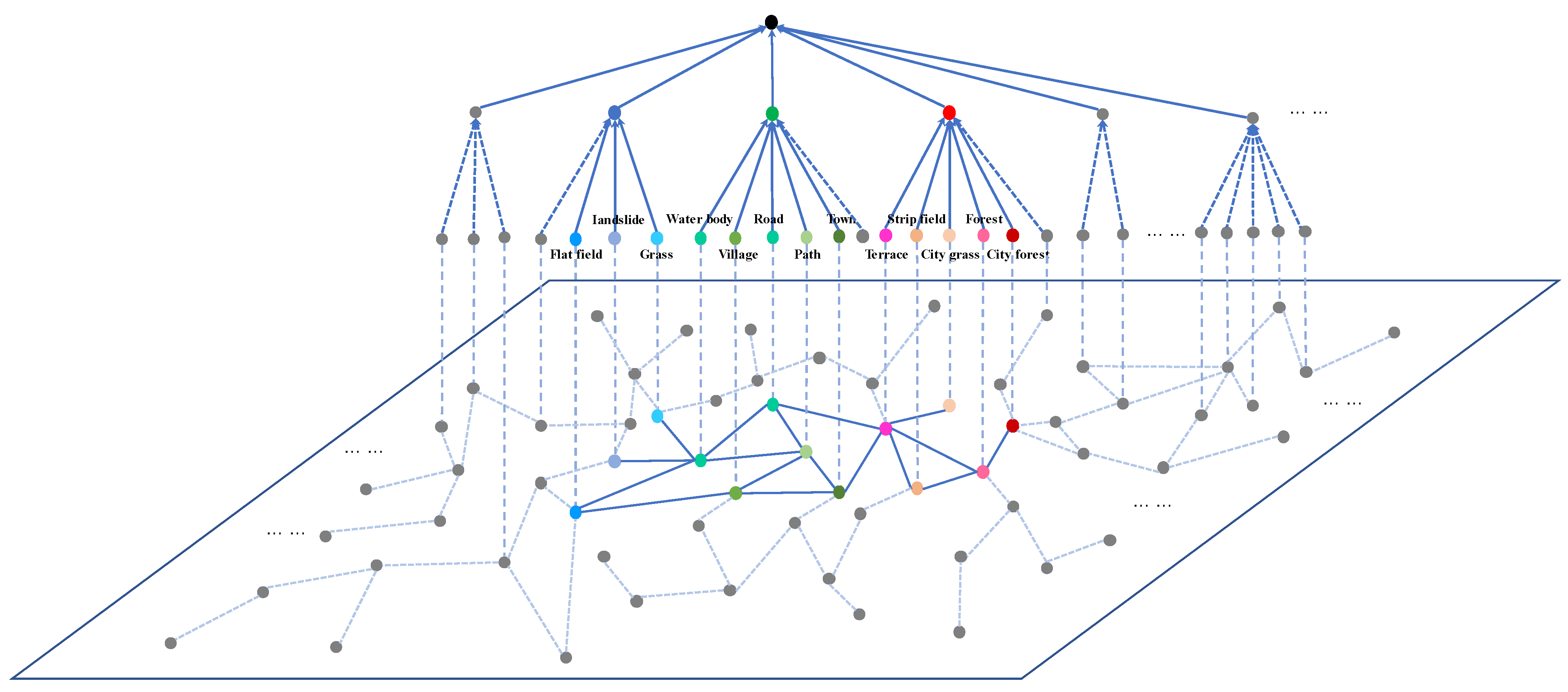
In Formulas (13) and (14), $n_{\alpha \beta }$ represents the number of samples that include categories $\alpha$ and $\beta$, $n_{\alpha }$ represents the number of samples that include category $\alpha$, and $n_{\beta }$ represents the number of samples that include category $\beta$. A large category system requires significant computational costs to search specific categories. The categories of different scenes are projected into the same plane, and the random walk algorithm in this plane can reduce the computational cost. Figure 5 shows the part of the knowledge graph.

(2)

The procedure of the parallel walking algorithm

In this algorithm, two anchor points are the start points of each walking path and are utilized to search the neighbor nodes in the knowledge graph. A first-cross-modality method and a second-cross-modality method are designed to integrate information from a different modality.

The neighbor node score is calculated based on the first-cross-modality method. In this method, the node features of the knowledge graph are the probability of corresponding categories in multilabel classification. The edges between nodes are still the cooccurrence probability derived from the knowledge graph. In this way, the walking algorithm integrates the symbiotic relationship between the visual information of the scene graph and the category information of the knowledge graph, which achieves the information fusion of visual modality and knowledge modality.

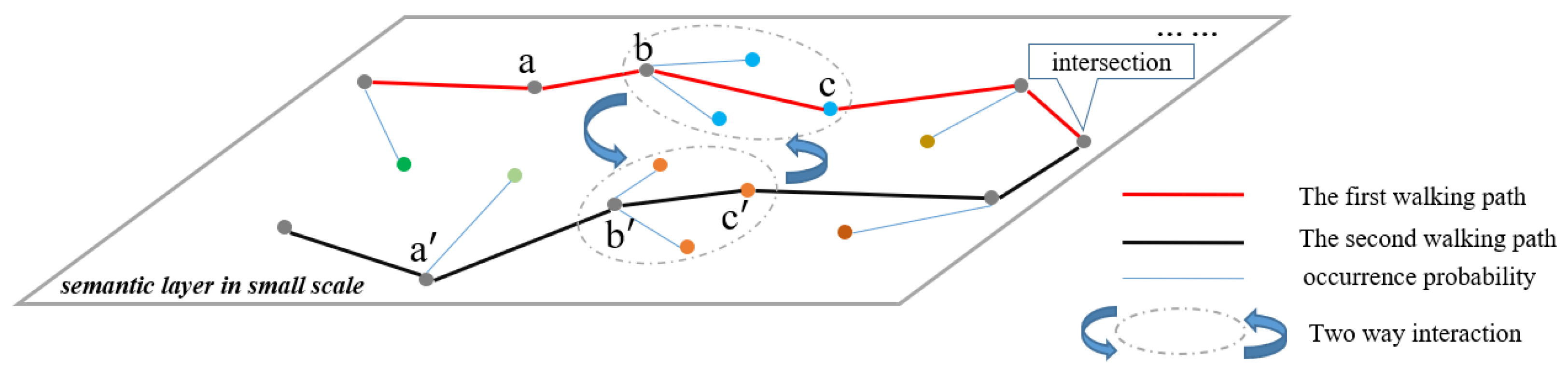
The neighbor node with the largest score is selected in the knowledge subgraph. The walking process moves to this node until the length of the path equals the number of superpixel groups in the scene graph or the path encounters a node from another scene. The node is called the valid junction node. The remote sensing object corresponding to this junction node is often the boundary between two different scenes. The knowledge subgraph is the union of respective experienced nodes after two paths terminate. The selection mechanism of the next node in the parallel walking algorithm is shown in Figure 6 below.

In Figure 6, a, b and c represent the previous node, the current node and the next node of the first walking path. ${\mathrm{a}}^{\prime }$, ${\mathrm{b}}^{\prime }$ and ${\mathrm{c}}^{\prime }$ represent the previous node, the current node and the next node of the second walking path, respectively.

$$Scor{e}_{\left(c\right)}=\lambda c{o}_{\left(bc\right)}\times p_{\left(c\right)}+\phi c{o}_{\left(b^{\prime }c\right)}\times p_{\left(c\right)}+\mu p_{\left(a\right)}$$

(15)

$$\lambda +\phi +\mu =1$$

(16)

Formula (15) shows the calculation of the neighbor score.

$c{o}_{\left(bc\right)}\times p_{\left(c\right)}$ represents the current node information of the first walking path, $c{o}_{\left(bc\right)}$ represents the cooccurrence probability of categories b and c.$p_{\left(c\right)}$ represents the next node score of the multilabel classification.

$c{o}_{\left(b^{\prime }c\right)}\times p_{\left(c\right)}$ represents the current node of $b^{\prime }$ information of the second walking path; $c{o}_{\left(b^{\prime }c\right)}$ represents the cooccurrence probability of category $b^{\prime }$ and category c.

$p_{\left(a\right)}$ represents the previous node score of multilabel classification.

$\lambda ,\phi ,\mu$ are hyperparameters, where $\lambda ,\phi ,\mu \in \left[0,1\right]$. $\lambda$ controls the influence of the current node. μ controls the influence of the previous node to avoid scene transition. As for the scene transition, after encountering the categories shared by the two scenes, the walking of one scene jumps to the scene corresponding to the other path in advance before traversing all the necessary category nodes, which may omit the nodes, resulting in an incomplete knowledge subgraph. The scene transition is explained in Section 4.1 in detail. $\phi$ controls the influence of the current node of the second walking path to achieve the interaction of the walking algorithm. From Formula (16), three hyperparameters sum to 1.

The scene graph—knowledge graph matching based on the parallel walking algorithm is denoted as follows:

Algorithm 1: Parallel walking algorithm for scene graph–knowledge graph matching.

Input: multilabel classification score (descending ranking): P,                cooccurrence probability matrix: M,                knowledge graph: $G_{kg}$,                Number of super pixel clusters in the sample scene graph: N    Output: $nodes$//node set of knowledge subgraph $G_{subkg}$

1 Begin

2 Initialize $nodes=\varnothing$, $firNodes=\varnothing$, $secNodes=\varnothing$, $firEndid=0$, $secEndid=0$, $count=0$

3 //Initialize the node set of knowledge subgraph, the node set of walking paths and the termination ID

4 $firNodes\leftarrow index\left(P\left[0\right]\right);$

5 //Store the node with the highest score in P as the starting point in $firNodes$, and $index$ is the node ID corresponding to the $P$ score

6 While $index\left(P\left[0\right]\right) and index\left(P\left[count+1\right]\right)$ in the same scene:

7 $count$ = $count$ + 1

8 $secNodes\leftarrow index\left(P\left[count+1\right]\right);$

9 //Store the second scoring node in P as the starting point in sec$Nodes$

10 For $i\leftarrow 0toN$ do: // When the scale of walking algorithm reaches m, the wandering ends.

11 $neiNodes1\leftarrow getNeiNodes\left(firNodes\left[i\right], G_{kg}\right);$

12 //Obtain the one hop neighbor node set $neiNodes1$ of first walking path of the i-th node in the knowledge graph $G_{kg}$

13 $neiNodes2\leftarrow getNeiNodes\left(secNodes\left[i\right], G_{kg}\right);$

14 //Obtain the one hop neighbor node set $neiNodes2$ of second walking path of the i-th node in the knowledge graph $G_{kg}$

15 $\mathrm{nei}Score1\leftarrow \mu c{o}_{\left(bc\right)}\times p_{\left(c\right)}+\left(\lambda -\mu \right)Z_{\left(a^{\prime }\right)}\times c{o}_{\left(b^{\prime }c\right)}\times p_{\left(c\right)}+\left(1-\lambda \right)p_{\left(a\right)};$

16 //Interactive calculation of the neighbor node score $neiScore1$ of node i in the first walking path.

17 $\mathrm{nei}Score2\leftarrow \mu c{o}_{\left(b^{\prime }{c}^{\prime }\right)}\times p_{\left(c^{\prime }\right)}+\left(\lambda -\mu \right)Z_{\left(a\right)}\times c{o}_{\left(b{c}^{\prime }\right)}\times p_{\left(c^{\prime }\right)}+\left(1-\lambda \right)p_{\left(a^{\prime }\right)};$

18 //Two-way interactive calculation of the neighbor node score $neiScore1$ of node i in the second walking path.

19 $firNodes\leftarrow index\left(Max\left(\mathrm{nei}Score1\right)\right);$

20 //Save the node ID with the highest score in $neiScore1$ into the node set of the first walking path

21 $secNodes\leftarrow index\left(Max\left(\mathrm{nei}Score2\right)\right);$

22 //Save the node ID with the highest score in $neiScore2$ into the node set of the second walking path

23 $crossNode\leftarrow firNodes\cap secNodes;$ //Save the intersection of two paths into $crossNode$

24 if $crossNode!=Null$ then

25 $firEndid\leftarrow index\left(crossNode\right);$ //Obtain the index of the intersection on the first walking path

26 $secEndid\leftarrow index\left(crossNode\right);$ //Obtain the index of the intersection on the second walking path

27 break; //Two ways intersect and the walking process ends.

28 $i\leftarrow i+1;$

29 End For

30 $nodes\leftarrow firNodes\left[:firEndid\left]\cup secNodes\right[:secEndid\right];$

31 //Combine the intersection of the walking path and the previous nodes to obtain the node set of the subgraph of the knowledge graph

32 Return $nodes$; //represent the node set of knowledge subgraph $G_{subkg}$

33 End

In Algorithm 1, the design of the termination condition of walking is restricted in two ways. First, the number of superpixel groups $N$ in the sample scene graph controls the size of the walking path. If the size of the walking path is equal to $N$, the walking algorithm ends, which avoids infinite process. Second, the walking process will be terminated early at the valid junctions. Moreover, the intersection procedure is an asynchronous process.

2.4. Semantic Classification Module for Superpixel Groups Based on Knowledge Subgraphs

This module achieves semantic classification of the superpixel groups based on second-cross-modality. In the second-cross-modality method—different from the first-cross-modality method, whose node feature is the multilabel classification score—the node feature of the knowledge graph is the word embedding feature of the categories. The embedding information is integrated with the visual information of the scene graph. Compared with applying the whole knowledge graph and the unoptimized sample scene graph, the semantic classification module greatly improves the model efficiency and accuracy. The structure of the superpixel group semantic classification module based on knowledge subgraphs is shown in Figure 7 below.

As shown in Figure 7, the input of this module is the final superpixel group feature $F_{group}$ and the knowledge subgraph $G_{subkg}$. The module is described in detail below:

2.4.1. Knowledge Subgraph Information Embedding

The mixed feature $F_{mixfg}$ of the final superpixel group is calculated by embedding the knowledge subgraph information into the final superpixel group feature, where $F_{mixfg}\in R^{N\times 2D}$. The formula of second-cross-modality is as follows:

$$F_{mixfg}=\left(Att\left(F_{group}, F_U\right)\times F_U\right)\parallel F_{group }$$

(17)

In Formula (17), $F_{mixfg}$ denotes the final mixed feature. $Att(.)$ denotes an attention function such as the cosine similarity between the nodes in the knowledge subgraph, as shown in Formula (5). $F_{group}$ denotes the final superpixel group feature. $F_{U }$ denotes the word embedding features of the nodes in the knowledge graph, where $F_U\in R^{K\times D}$ and K is the number of nodes in the knowledge subgraph. ‘$\parallel$’ denotes the concatenate function.

2.4.2. Feature Aggregation through GAT

The final updated mixed feature of superpixel group $F{\prime }_{mixfg}$ is obtained from GAT with the final mixed feature of superpixel group $F_{mixfg}$, where $F{\prime }_{mixfg}\in R^{N\times 2D}$. The formula is as follows:

$$F{\prime }_{mixfg}=GAT\left(F_{mixfg}\right)$$

(18)

In Formula (18), $F{\prime }_{mixfg}$ denotes the final mixed updated feature of the superpixel group.

2.4.3. Semantic Classification of Superpixel Groups

$F{\prime }_{mixfg}$ is fed into a special classifier, which freezes the remaining category nodes by knowledge graph category mask matrix $\mathrm{kgMask}$, where $kgMask\in R^{2D\times C}$. The frozen category nodes are not in the knowledge subgraph. In this way, this classifier can improve the classification performance. The calculation formula is as follows:

$$kgMas{k}_{\left(d,\beta \right)}=\{\begin{array}{c}1, \beta \in G_{subkg}\\ 0, \beta \notin G_{subkg}\end{array}$$

(19)

In Formula (19), $kgMas{k}_{\left(d,\beta \right)}$ shows the value of the d-th dimension and the β-th category in the knowledge graph category mask matrix. If β belongs to the knowledge subgraph, $kgMas{k}_{\left(d,\beta \right)}$ is 1, otherwise it is 0. The classification formula is as follows:

$$Output=softmax\left(F{\prime }_{mixfg}\times W\circ kgMask\right)$$

(20)

In Formula (20), $Output$ denotes the result of classification.$F{\prime }_{mixfg}$ denotes the final mixed updated feature of the superpixel group. $W$ denotes the training weight, $\prime \circ \prime$ denotes the Hadamard product, and $\prime \times \prime$ denotes matrix multiplication.

The following formula shows cross entropy loss function ${\mathcal{L}}_{semantic}$ of the superpixel groups’ semantic classification:

$${\mathcal{L}}_{semantic}=-\frac{1}{N}{{\displaystyle \sum }}_i^N{y}_i\ast log\widehat{y_i}$$

(21)

In Formula (21), $y$ denotes the label of the superpixel groups’ semantic classification, where $\mathrm{y}\in R^{N\times 1}$. $\widehat{y}$ denotes the prediction result of the superpixel groups’ semantic classification. $N$ is the number of superpixel groups.

3. Results

3.1. Introduction of Research Areas and Samples

The research area is part of Wenchuan County, Sichuan Province. The latitude range of this area is from 30°45′ to 31°43′ and the longitude range is from 102°51′ to 103°44′. The remote sensing image used in this study is the historical Google Earth image in August 2008, of which the spatial resolution is 0.59 m and the number of bands is three.

The experimental dataset includes 1625 samples that are randomly divided into a training set and a test set at a ratio of 3:1. Each sample contains a remote sensing image, a labelled image and an object mask image with the same size of 224 × 224 pixels.

The knowledge graph in this paper is constructed from classification criteria, which contain 181 categories and 529 relations.

3.2. Network Parameters

The training settings of Unet are as follows: the underlying feature dimension is set to 512, and the batch size is set to 32.

The training settings of both the GAT and KGGAT [1] networks are as follows: the hidden dimension is 128, the number of GAT layers is set to 2 and the batch size is set to 1. Moreover, KGGAT (Knowledge Graph Attention Network) combines the whole knowledge graph information with the graph attention network and is used for the semantic segmentation task of superpixel objects.

The training settings of our PWGM model are as follows: the dimension of visual features from the backbone is 64 and the batch size is set to 1.

The classifier dimension of the above models is set to 30, the learning rate is set to 3 × 10⁻⁴, the training epoch is 300 and the Adam optimizer is used in the training process. We conducted all the experiments on RTX3080.

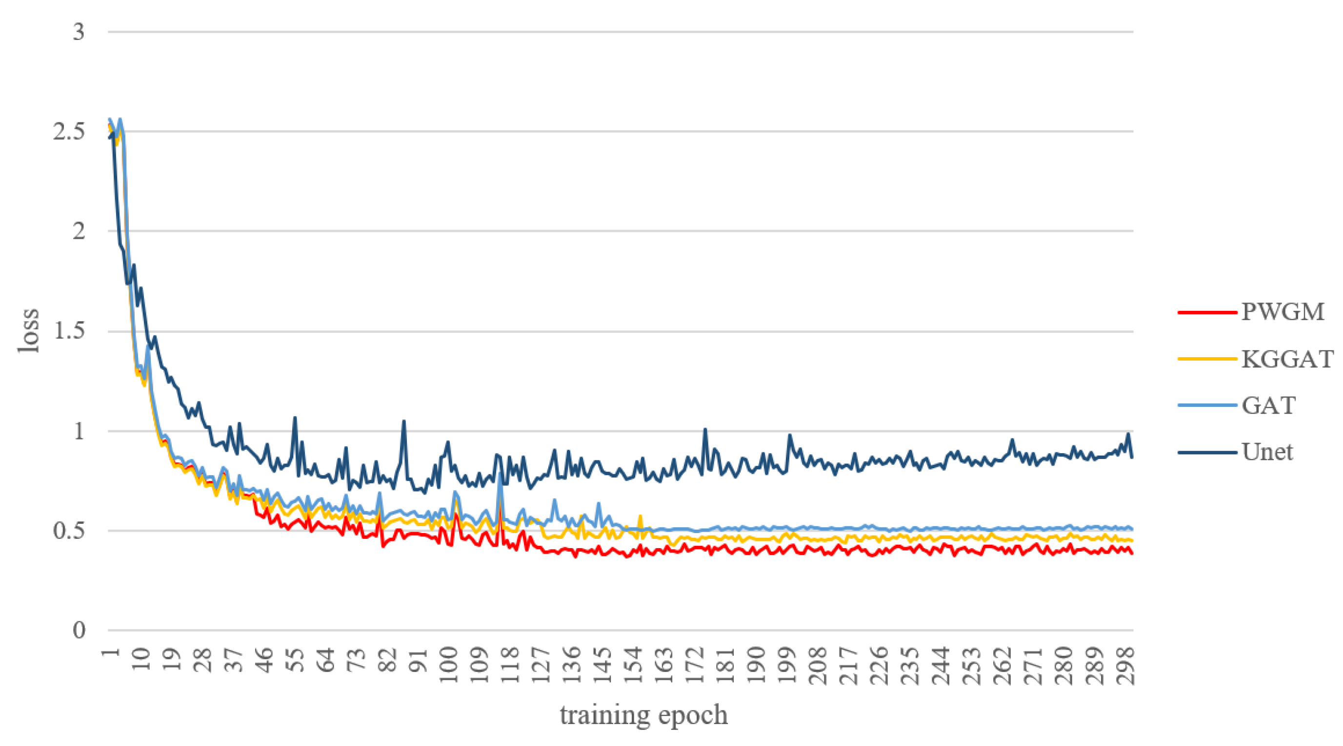
3.3. Loss Curve

The loss curve of the above models in the test set is shown in Figure 8 below.

In Figure 8, the y-axis represents the loss value of the test set during training and the x-axis represents the training epochs. It shows the loss curve of the test set of PWGM, KGGAT, GAT, and Unet.

The initial losses of the four models are all approximately 2.5. The loss fluctuates significantly in the early stage and stabilizes in the later stage. More specifically, the loss of the Unet and GAT models remains stable from the 200th epoch and 144th epoch while for the KGGAT model and our PWGM model, the loss stabilizes when the training epochs reach 169 and 122, respectively. The result directly shows that PWGM using the knowledge subgraph more easily converges than KGGAT using the whole knowledge graph.

In addition, after the loss becomes stable, our PWGM shows the lowest loss value, which also reflects its excellent performance in the test set.

3.4. Model Classification Precision Analysis

This section compares the four models with four semantic segmentation metrics, including overall accuracy (OA), mean intersection over union (mIoU), Kappa coefficient, and F1-Score. The results are shown in the following

Table 4. The OA, mIoU, Kappa, and F1-Score of four networks.

	OA	mIoU	Kappa	F1-Score
Unet	0.796	0.635	0.778	0.713
GAT	0.878	0.801	0.862	0.890
KGGAT	0.897	0.820	0.885	0.892
PWGM (Ours)	0.929	0.853	0.920	0.923

:

As is shown in Table 4, PWGM performs best in the four metrics, which shows its highest precision in the test set.

The accuracy of the object-based GNN is significantly higher than that of the pixel-based Unet. The OA of PWGM is 92.9% and those of KGGAT, GAT and Unet are 89.7%, 87.8% and 79.6%, respectively.

The OAs of PWGM, KGGAT and GAT are 13.3%, 10.1% and 8.2% higher than that of Unet, respectively. Compared with GAT, the OA of PWGM and KGGAT is improved by 5.1% and 1.9%, respectively. In addition, the OA of PWGM is 3.2% higher than that of KGGAT.

From the comparison results, we can obtain the following conclusions:

• The object-based GNNs outperform the pixel-based Unet in the above metrics.
• PWGM and KGGAT integrated with knowledge information perform better than GAT;
• PWGM with the knowledge subgraph surpasses KGGAT with the whole knowledge graph.

The results of the pixel confusion matrix in the test set are as follows:

Table 5. The pixel-based classification confusion matrix of Unet.

	Flat Field	Landslide	Grass	Water Body	Village	Road	Path	Town	Terrace	Strip Field	City Grass	Forest	City Forest	Sum of Pixel	Accuracy
flat field	1,795,560	1960	46,141	0	96,535	384	13,023	1748	13,098	461	15	44,768	130	2,013,823	0.891
landslide	4580	2,241,286	164,516	35,051	19,178	15,028	19,650	13,532	9295	10,167	7503	104,177	1334	2,645,297	0.847
grass	106,861	145,475	1,808,823	58,420	181,062	32,265	23,533	44,042	116,883	33,267	33,731	274,054	12,880	2,871,296	0.629
water body	972	18,642	28,330	1,371,473	2167	11,214	6	9207	1062	590	5112	6035	1801	1,456,611	0.941
village	92,896	2602	74,016	3927	1,238,335	7329	12,876	102,389	8146	6975	4642	147,308	5675	1,707,116	0.725
road	858	16,843	14,393	15,741	7393	152,166	3868	56,565	77	158	4504	3339	1409	277,314	0.548
path	25,255	18,275	17,185	4	36,583	5569	140,362	7878	9974	9176	33	8589	75	278,958	0.503
town	216	7003	11,177	13,718	72,131	24,440	101	1,522,105	0	18	28,560	35,469	41,879	1,756,817	0.866
terrace	53,041	1949	66,821	420	25,583	152	14,894	66	1,329,939	45,428	176	86,662	8	1,625,139	0.818
strip field	29,573	636	28,184	795	9033	195	10,505	45	40,645	1,684,747	419	48,252	3	1,853,032	0.909
city grass	651	486	23,239	8752	6151	6389	127	28,094	0	9	31,922	18,352	21,579	145,751	0.219
forest	50,139	65,758	247,138	8712	164,772	2277	5226	12,698	37,719	50,944	8855	3,451,530	31,395	4,137,163	0.834
city forest	2658	996	9136	4543	3119	1916	39	27,834	0	104	12,970	42,667	80,197	186,179	0.430

,

Table 6. The pixel-based classification confusion matrix of GAT.

	Flat Field	Landslide	Grass	Water Body	Village	Road	Path	Town	Terrace	Strip Field	City Grass	Forest	City Forest	Sum of Pixel	Accuracy
flat field	1,730,815	5368	195,214	5325	24,563	1353	8085	0	26,665	0	0	16,434	0	2,013,823	0.859
landslide	0	2,440,442	155,939	174	11,845	17,897	6523	832	0	0	4453	7191	0	2,645,297	0.922
grass	32,385	83,124	2,125,012	70,160	64,089	6196	6776	5605	87,151	66,073	22,039	265,881	36,805	2,871,296	0.740
water body	0	9801	178,107	1,259,104	233	7377	0	0	0	0	1988	0	0	1,456,611	0.864
village	13,902	28,614	44,088	10,312	1,530,321	1443	3663	2382	3122	45,761	2508	20,907	93	1,707,116	0.896
road	0	6431	1267	1546	12,057	214,633	10,225	29,362	0	0	1792	0	0	277,314	0.773
path	10,354	14,579	25,524	0	9076	2405	207,048	5783	0	820	0	3369	0	278,958	0.742
town	0	1288	8762	2778	160,059	11,771	369	1,499,408	0	0	31,389	14,305	26,688	1,756,817	0.853
terrace	29,411	0	47,731	2432	2020	0	226	0	1,443,793	21,769	0	77,757	0	1,625,139	0.888
strip field	0	2465	10,189	0	4051	0	571	0	12,771	1,799,280	0	23,705	0	1,853,032	0.970
city grass	0	5576	56,948	5248	2566	2026	0	4267	0	0	51,012	4085	14,023	145,751	0.350
forest	14,881	9140	444,613	0	21,741	1225	0	2244	12,945	46,345	0	3,510,969	73,060	4,137,163	0.848
city forest	0	0	3693	0	0	0	0	11,763	0	5509	0	46,737	118,477	186,179	0.636

,

Table 7. The pixel-based classification confusion matrix of KGGAT.

	Flat Field	Landslide	Grass	Water Body	Village	Road	Path	Town	Terrace	Strip Field	City Grass	Forest	City Forest	Sum of Pixel	Accuracy
flat field	1,859,030	5368	67,272	5325	24,563	1353	7813	0	26,665	0	0	16,434	0	2,013,823	0.923
landslide	0	2,571,005	27,091	174	11,845	16,183	6523	832	0	0	4453	7191	0	2,645,297	0.972
grass	15,003	88,590	2,317,620	70,160	61,935	2950	5941	5605	87,151	55,245	22,039	112,018	27,039	2,871,296	0.807
water body	0	9801	18,394	1,418,818	233	7377	0	0	0	0	1988	0	0	1,456,611	0.974
village	13,902	28,614	34,019	10,312	1,546,318	1443	3663	39,263	3122	3125	2508	20,827	0	1,707,116	0.906
road	0	6431	1267	1546	8057	239,535	10,225	8461	0	0	1792	0	0	277,314	0.864
path	12,697	11,397	24,016	0	19,076	10,060	191,740	5783	0	820	0	3369	0	278,958	0.687
town	0	1288	8762	2778	40,203	6102	369	1,625,390	0	0	31,389	14,305	26,231	1,756,817	0.925
terrace	29,411	0	77,731	2432	2020	0	226	0	1,410,698	21,769	0	80,852	0	1,625,139	0.868
strip field	0	2465	20,189	0	14,051	0	571	0	2053	1,756,553	0	57,150	0	1,853,032	0.948
city grass	0	5576	13,321	5248	2566	2026	0	14,267	0	0	83,515	7033	12,199	145,751	0.573
forest	9951	9140	214,321	0	21,539	1225	0	2244	12,945	33,414	0	3,763,354	69,030	4,137,163	0.910
city forest	0	0	13,693	0	0	0	0	11,763	0	5509	0	22,289	132,935	186,179	0.714

and

Table 8. The pixel-based classification confusion matrix of PWGM.

	Flat Field	Landslide	Grass	Water Body	Village	Road	Path	Town	Terrace	Strip Field	City Grass	Forest	City Forest	Sum of Pixel	Accuracy
flat field	1,893,895	5368	59,827	5325	17,209	852	6205	0	9311	0	0	15,831	0	2,013,823	0.940
landslide	0	2,573,213	28,624	174	10,662	16,183	6073	832	0	0	2345	7191	0	2,645,297	0.973
grass	10,655	58,342	2,512,137	16,401	33,411	1558	1187	5605	56,699	11,583	1915	146,989	14,814	2,871,296	0.875
water body	0	2065	21,887	1,425,049	233	7377	0	0	0	0	0	0	0	1,456,611	0.978
village	13,902	18,639	26,863	10,248	1,598,267	1088	2768	14,071	408	3125	2358	15,379	0	1,707,116	0.936
road	0	5898	1267	643	12,057	245,738	7018	4693	0	0	0	0	0	277,314	0.886
path	12,697	15,389	16,741	0	13,853	0	210,639	5783	0	487	0	3369	0	278,958	0.755
town	0	1288	7974	2390	13,520	6102	369	1,661,090	0	0	31,389	6464	26,231	1,756,817	0.946
terrace	28,102	0	34,449	2432	2020	0	0	0	1,466,610	8484	0	83,042	0	1,625,139	0.903
strip field	0	0	0	0	14,051	0	0	0	1280	1,823,359	0	14,342	0	1,853,032	0.984
city grass	0	451	22,298	2327	2566	74	0	12,750	0	0	55,645	12,041	37,599	145,751	0.382
forest	9951	6581	155,856	0	20,331	1225	0	98	2041	28,826	0	3,865,463	46,791	4,137,163	0.934
city forest	0	0	13,448	0	0	0	0	11,422	0	5509	0	9129	146,671	186,179	0.788

are the confusion matrices of Unet, GAT, KGGAT and PWGM, respectively.

To illustrate the advantages of PWGM in more detail, we compare them from the classification accuracy of each category in the confusion matrix. The results are shown as follows in

Table 9. The accuracies of each category in four networks.

	Flat Field	Landslide	Grass	Water Body	Village	Road	Path	Town	Terrace	Strip Field	City Grass	Forest	City Forest
Unet	0.891	0.847	0.629	0.941	0.725	0.548	0.503	0.866	0.818	0.909	0.219	0.834	0.430
GAT	0.859	0.922	0.740	0.864	0.896	0.773	0.742	0.853	0.888	0.970	0.350	0.848	0.636
KGGAT	0.923	0.972	0.807	0.974	0.906	0.864	0.687	0.925	0.868	0.948	0.573	0.91	0.714
PWGM	0.940	0.973	0.875	0.978	0.936	0.886	0.755	0.946	0.903	0.984	0.702	0.934	0.788

:

As shown in Table 9, the accuracy of each category of PWGM is higher than that of any other model. We can also obtain the following conclusions:

• PWGM greatly expands the receptive field through the graph structure, which solves the problem of the limited receptive field in Unet. Compared with Unet, the accuracy of each category of PWGM is increased by 18.77% on average.
• PWGM integrates background information into samples based on a knowledge graph. Due to the added background information, the accuracy of each category of PWGM is increased by 9.68% on average compared with GAT.
• PWGM obtains precise knowledge subgraphs through graph matching and applies them to the scene segmentation of remote sensing. This method improves the classification accuracy because of the added whole knowledge graph information. Compared with KGGAT, the accuracy of each category of PWGM is increased by 4.07% on average. This shows that applying knowledge subgraphs is more effective than the whole knowledge graph for classification.

3.5. Model Robustness Analysis

The stability of the models is related to reproducibility. Therefore, it is necessary to verify the stability of PWGM. First, the original dataset is randomly assigned 10 times to obtain 10 new train and test parts. Secondly, we conduct 10 independent Monte Carlo experiments based on these parts. Finally, we compare OA, mIoU, Kappa and F1-Score on the test set. The results are shown in Figure 9.

In Figure 9, the x-axis represents the experimental index, and the y-axis represents the metric value. The average values of the above metrics are 0.9269, 0.8509, 0.9189 and 0.9209, respectively, which are close to the previous experimental results of PWGM. Moreover, the standard deviations of the four metric values are 0.00247, 0.00243, 0.00249 and 0.00259. The above analysis shows that PWGM is robust and stable and that the experimental results are repeatable.

3.6. Model Performance Test

When analyzing the advantages of PWGM, we compare the model parameters, GPU memory cost, average single training time and total training time in 300 epochs. The results are shown in

Table 10. The performance of four networks.

Model	Parameters (M)	GPU Memory Cost (G)	Average Training Time per Epoch (S)	Total Training Time (Min)
Unet	8.64	8.88	40	200
GAT	0.02	1.47	24	120
KGGAT	0.02	1.51	30	150
PWGM	0.02	0.88	15	75

.

As shown in Table 10, the following conclusions can be drawn:

(1)

The model parameters of the GNNs are all 0.02 M, which is much smaller than that of Unet. This shows that the object-based GNN is extremely light.

(2)

The GPU memory cost of PWGM is 0.88 G. Compared with Unet, the cost is reduced by 1/10. Compared with KGGAT based on the whole knowledge graph, the cost is reduced by 0.63 G.

(3)

The single average training time and total training time of PWGM are also much lower than those of Unet and KGGAT.

In conclusion, the results show that PWGM has obvious advantages in efficiency.

3.7. Clustering Threshold Analysis

When designing a clustering graph pooling method, it is necessary to set a clustering threshold, which is mainly used for clustering, and the value ranges from 0 to 1. The clustering threshold of PWGM in this paper is set to 0.75. We design experiments to compare the results with different clustering thresholds, which increase from 0.2 to 0.95 in steps of 0.05. Then, we analyze the experimental results in two indicators of clustering homogeneity and object reduction rate. After clustering and pooling, superpixels are clustered into superpixel groups. This reduces the number of objects.

As shown in Table 11, this can be concluded as follows.

(1)

The clustering homogeneity has great influence on the classification accuracy, and the object reduction rate greatly affects the model efficiency. When the clustering threshold is set to 0.2, the object reduction rate is highest, but the clustering homogeneity is the lowest. However, when the clustering threshold is set from 0.8 to 0.95, the clustering homogeneity appears to be the opposite, causing low efficiency.

(2)

We pay more attention to clustering homogeneity because the classification accuracy is more critical. Therefore, the clustering threshold is finally set to 0.75, the clustering homogeneity is 0.964 and the object reduction rate is 33.60.

Table 11. The experimental results with different clustering thresholds.

Iteration End Value	Number of Same Groups	Number of Groups after Clustering	Clustering Homogeneity	Number of Objects	Number of Reduced Objects	Object Reduction Rate (%)
0.2	662	1060	0.624	6264	5204	83.08
0.25	731	1124	0.650	6264	5140	82.06
0.3	789	1184	0.666	6264	5080	81.10
0.35	856	1246	0.687	6264	5018	80.11
0.4	953	1338	0.713	6264	4926	78.64
0.45	1049	1429	0.734	6264	4835	77.19
0.5	1165	1538	0.757	6264	4726	75.45
0.55	1394	1748	0.797	6264	4516	72.09
0.6	1685	2015	0.836	6264	4249	67.83
0.65	2113	2413	0.876	6264	3851	61.48
0.7	2764	3020	0.915	6264	3244	51.79
0.75	4003	4159	0.964	6264	2105	33.60
0.8–0.95	6264	6264	1.0	6264	0	0.00

Note: Clustering homogeneity = number of same groups/number of groups after clustering. Object reduction rate = number of reduced objects/number of objects.

Table 11. The experimental results with different clustering thresholds.

Iteration End Value	Number of Same Groups	Number of Groups after Clustering	Clustering Homogeneity	Number of Objects	Number of Reduced Objects	Object Reduction Rate (%)
0.2	662	1060	0.624	6264	5204	83.08
0.25	731	1124	0.650	6264	5140	82.06
0.3	789	1184	0.666	6264	5080	81.10
0.35	856	1246	0.687	6264	5018	80.11
0.4	953	1338	0.713	6264	4926	78.64
0.45	1049	1429	0.734	6264	4835	77.19
0.5	1165	1538	0.757	6264	4726	75.45
0.55	1394	1748	0.797	6264	4516	72.09
0.6	1685	2015	0.836	6264	4249	67.83
0.65	2113	2413	0.876	6264	3851	61.48
0.7	2764	3020	0.915	6264	3244	51.79
0.75	4003	4159	0.964	6264	2105	33.60
0.8–0.95	6264	6264	1.0	6264	0	0.00

Note: Clustering homogeneity = number of same groups/number of groups after clustering. Object reduction rate = number of reduced objects/number of objects.

4. Discussion

In this chapter, we analyze the efficacy of each factor in the Scene Graph—Knowledge Graph Matching Module based on the parallel walking algorithm and reveal the working principle. First, we explain the termination condition and evaluation metrics of the parallel walking.

The definition of the termination condition is as follows:

(1)

When the category node encountered by the walking path of the current scene derives from another scene and only belongs to this scene, this category node is the valid junction node. In this situation, the parallel walking algorithm ends. It is worth noting that if the two scenes both contain the category, the walking algorithm does not end.

(2)

When the number of path nodes is the same as the number of nodes in the pooled scene graph, parallel walking ends.

The parallel walking ends when either condition is satisfied.

On this basis, two evaluation metrics are designed to evaluate the algorithm, which are named the intersection rate and the parallel walking accuracy rate. The intersection rate refers to the proportion of the number of intersection samples in a test set. The formula for calculating this is as follows:

$$meetRate=\frac{Num\left(meetSamples\right)}{Num\left(allSamples\right)}$$

(22)

In Formula (22), $meetRate$ denotes the intersection rate and $Num(.)$ is a counting method. $meetSamples$ is a sample set for achieving parallel walking intersection.

The parallel walking accuracy rate is the ratio of correct predictions compared to GT. The calculating formula is as follows:

$$walkAcc=\frac{Num\left(walkPre\cap walkLabel\right)}{Num\left(walkLabel\right)}$$

(23)

In Formula (23), $walkAcc$ denotes the walking accuracy. $walkPre$ is the actual result of a node set when parallel walking ends. $walkLabel$ denotes the label of nodes during the walking algorithm (GT).

Table 12. Scene distribution statistics of double anchors in a test set.

Scene Type	Number of Complex Scene Samples	Number of Scenes with Anchors in the Same Scene	Number of Scenes with Anchors in Different Scenes
Simple scene	165	165	0
Complex scene	260	0	260

shows the scene distribution statistics of double anchors in a test set. In simple scenes, anchors are in the same scene, while in complex scenes, the anchors are in different scenes.

4.1. The Influence of the Solidified Factor

In some complex scene samples, parallel walking starts from their respective anchor points and walks in two different scenes. When common scene categories appear during the walking process, the walking node leaves the initial path and the scene type changes. If the walking path does not reach the valid junction at this time, it may lead to the omission of some category nodes. This may reduce the walking accuracy.

Therefore, we introduce the multilabel classification score of the previous node (with $p_{\left(a\right)}$ as the solidified factor) and try to keep the algorithm moving steadily in the initial scene. The score can effectively avoid losing category nodes due to scene conversion until reaching the valid junction. In this way, the scene can be fixed to avoid losing category nodes due to scene transition and the scene graph–knowledge graph matching accuracy can be guaranteed. The experimental results are shown in

Table 13. Statistical results of the ablation experiment of $p_{\left(a\right)}$.

Factor Combination	Number of Landslide-Influenced Scenes	Number of Samples in Solidified Walking Scene	Number of Unresolved Samples	Scene Solidified Rate (%)
$c{o}_{\left(bc\right)}\times p_{\left(c\right)}$	81	21	60	32.1
$\lambda c{o}_{\left(bc\right)}\times p_{\left(c\right)}+\mu p_{\left(a\right)}$	81	73	8	90.1

Note: Scene solidified rate = number of samples in solidified walking scene/number of total samples.

.

In Table 13, the introduction of the factor $p_{\left(a\right)}$ has a greater impact on the fixation of the scene type, and the scene solidified rate is increased from 32.1% to 90.1%. The relevant samples are listed in Figure 10 below to verify its effect.

As shown in Table 14, it can be concluded as follows.

(1)

The parallel walking process ends when two paths meet at the road category (No. 6). As for the result of $c{o}_{\left(bc\right)}\times p_{\left(c\right)}$, the starting point of the first walking path is the village category (No. 5) and ending point is the landslide category (No. 2). When it walks to the same category, landslide (No. 2), the scene changes from village to urban. This phenomenon results in the lack of a dirt road category (No. 7) and grass category (No. 3) after the intersection.

(2)

It is of great help for differentiating the results of the two-way walking and improving the accuracy of the walking to consider previous node information. $\lambda c{o}_{\left(bc\right)}\times p_{\left(c\right)}+\mu p_{\left(a\right)}$ introduces the solidified factor $p_{\left(a\right)}$, which considers the information of the previous category node, forest (No. 12). The factor avoids the scene change that occurs in the first path to ensure the correctness of walking.

Table 14. Comparative analysis results of $p_{\left(a\right)}$.

Factor Combination	True Path	Number of Groups	First Walking Path	Second Walking Path	Intersection Category	Accuracy of the First Walking Path
$c{o}_{\left(bc\right)}\times p_{\left(c\right)}$	2, 3, 4, 5, 6, 7, 8, 11, 12, 13	10	5, 12, 2, 8, 13, 11, 4, 6, 7, 3	8, 13, 11, 4, 6, 7, 12, 5, 3, 2	Road(6)	0.80
$\lambda c{o}_{\left(bc\right)}\times p_{\left(c\right)}+\mu p_{\left(a\right)}$	2, 3, 4, 5, 6, 7, 8, 11, 12, 13	10	5, 12, 2, 7, 3, 6, 11, 13, 4, 8	8, 13, 11, 4, 6, 7, 12, 5, 3	Road(6)	1.0

Note: Categories in blue belong to the rural scene and categories in yellow belong to the urban scene. The category in red is the valid junction node.

Table 14. Comparative analysis results of $p_{\left(a\right)}$.

Factor Combination	True Path	Number of Groups	First Walking Path	Second Walking Path	Intersection Category	Accuracy of the First Walking Path
$c{o}_{\left(bc\right)}\times p_{\left(c\right)}$	2, 3, 4, 5, 6, 7, 8, 11, 12, 13	10	5, 12, 2, 8, 13, 11, 4, 6, 7, 3	8, 13, 11, 4, 6, 7, 12, 5, 3, 2	Road(6)	0.80
$\lambda c{o}_{\left(bc\right)}\times p_{\left(c\right)}+\mu p_{\left(a\right)}$	2, 3, 4, 5, 6, 7, 8, 11, 12, 13	10	5, 12, 2, 7, 3, 6, 11, 13, 4, 8	8, 13, 11, 4, 6, 7, 12, 5, 3	Road(6)	1.0

Note: Categories in blue belong to the rural scene and categories in yellow belong to the urban scene. The category in red is the valid junction node.

4.2. The Influencing of the Intersection Factor

The two walking paths traverse the initial scene corresponding to the anchor points, respectively, and they select the category nodes that match the features of the sample in the knowledge graph. If the mechanism of early termination is not designed, each walking path lasts until the number of walking nodes equals the number of nodes in the optimized scene graph. In this way, the knowledge subgraph contains redundant nodes.

It is expected that the path ends at a valid junction before traversing all N steps and avoids the interference of redundant nodes. Thus, we design an intersection factor, $c{o}_{\left(b^{\prime }c\right)}$, to enhance the rationality of the valid junction. The impact of the intersection factor on the model is analyzed from efficiency and accuracy below.

4.2.1. Model Efficiency

For the intersection factor: $c{o}_{\left(b^{\prime }c\right)}$, its effect on model efficiency is shown by the following experiments, where different combinations are utilized to calculate the walking score of the next node in the parallel walking algorithm:

As shown in

Table 15. Experimental results of the influence of the intersection factor on the parallel walking algorithm.

Method	Number of Complex Scene Samples	Number of Intersection Samples	Intersection Rate
$c{o}_{\left(bc\right)}\times p_{\left(c\right)}$	260	143	0.550
$\lambda c{o}_{\left(bc\right)}\times p_{\left(c\right)}+\mu p_{\left(a\right)}$	260	143	0.550
$\lambda c{o}_{\left(bc\right)}\times p_{\left(c\right)}+\phi c{o}_{\left(b^{\prime }c\right)}\times p_{\left(c\right)}+\mu p_{\left(a\right)}$	260	260	1.000

, $c{o}_{\left(b^{\prime }c\right)}$ represents the information of the second walking path, which achieves the information interaction. ${\mathrm{b}}^{\prime }$ is the current node of the second path and c is the next node in the first path. The factor achieves information exchange and greatly improves the intersection rate from 0.550 to 1.000. Additionally, the intersection category of walking is also the boundary of the complex scene samples.

Table 16. Statistical results of samples in which the intersection category separates different scenes.

Method Type	Number of Complex Scene Samples	Number of Scenes in Which the Intersection Separates Different Scenes	Ratio of Scenes in Which the Intersection Separates Different Scenes	Walking Accuracy before Intersection
$\lambda c{o}_{\left(bc\right)}\times p_{\left(c\right)}+\mu p_{\left(a\right)}$	260	143	0.550	0.803
$\lambda c{o}_{\left(bc\right)}\times p_{\left(c\right)}+\phi c{o}_{\left(b^{\prime }c\right)}\times p_{\left(c\right)}+\mu p_{\left(a\right)}$	260	260	1.000	0.962

shows the parallel walking results of the complex scene. We focus on two complex scenes, urban–rural and landslide-influenced, to conduct the case analysis. The total number of mixed samples corresponding to the complex scene is 260. The number of scenes in which the intersection category separates different scenes is 260, accounting for 100%. The intersection category of the walking process is also the boundary of the complex scene.

Table 17. Ablation experiment of terminating condition based on valid junction.

Valid Junction in Termination Condition	Number of Complex Samples	Number of Knowledge Subgraph Nodes	Reduction Comparison
No	260	2730	0
YES	260	2043	25.2%

Note: Reduction comparison = 25.2% = (2730 − 2043)/2730 × 100%.

shows the effectiveness of the valid junction. By applying the valid junction to the termination condition, the number of knowledge subgraph nodes is reduced from 2730 to 2043 (25.2%). In this way, the parallel walking algorithm reduces node redundancy and improves the model efficiency.

4.2.2. Model Accuracy

The knowledge subgraph considering the valid junction reduces the redundant category nodes, not only raising the efficiency of scene graph–knowledge graph matching, but also greatly improving the accuracy of sample segmentation from 80.3% to 96.2%, as shown in Table 16.

The actual samples are listed as follows to analyze the influence of the intersection on the segmentation accuracy of the sample scene.

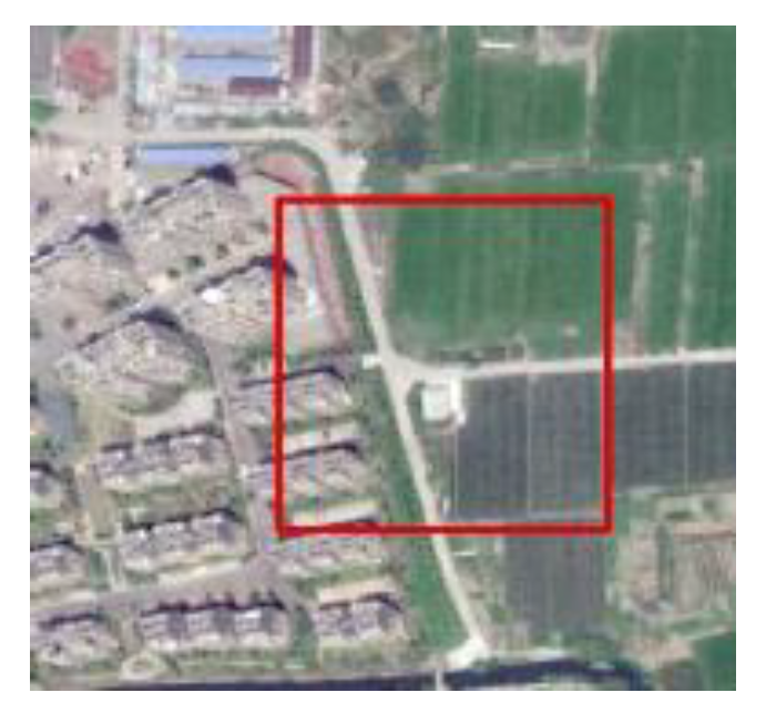
Figure 11 shows the example (red box) located in the specific scene. The categories within it include town, grass, city grass, village, flat field and path. This sample involves the phenomenon of “different objects with the same spectrum” between grass and city grass.

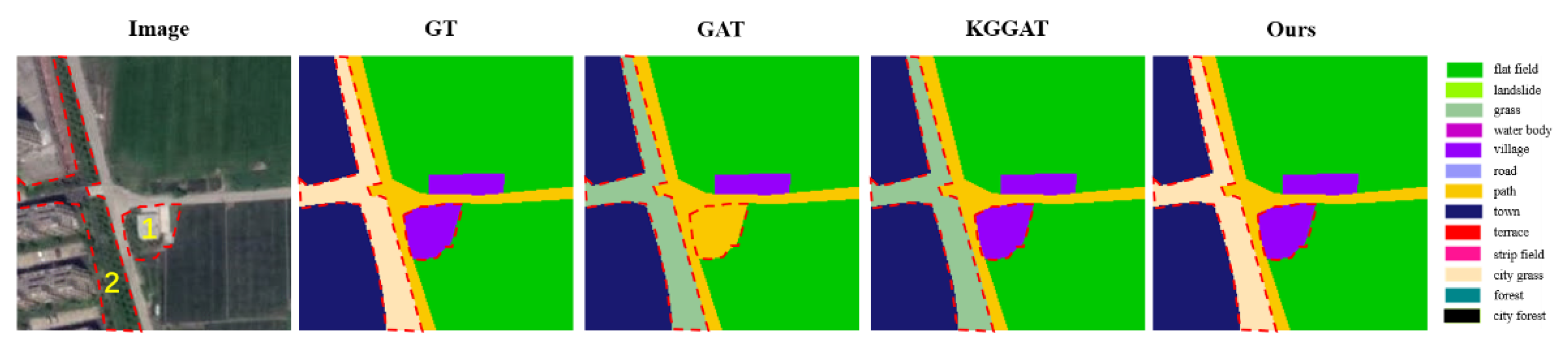
• Comparative analysis of GAT and KGGAT predictions of the sample

In Figure 12, the prediction of object 1 is different between GAT and KGGAT. The label of object 1 is village. GAT incorrectly predicts object 1 as path. The spectral and texture features of object 1 are similar to path, so the model adds the surrounding path features to object 1 with a large weight overlap. This results in the incorrect prediction of GAT. However, KGGAT applies knowledge information to accurately predict object 1 as village, because the model considers the knowledge graph based on the cooccurrence probability. From GT, the neighbor category of object 1 is flat field. It’s worth noting that the proportion of relevant pixels in rural scene is larger than that in the urban scene from

Table 18. Pixel proportion of category in sample II.

Category	Flat Field	Town	City Grass	Path	Village
Proportion	56%	21%	10%	8%	5%

. From

Table 19. Relevant cooccurrence probability for the analysis of object 1.

Category	Flat Field	Road	Village
village	0.81	0.42	1.00
path	0.58	1.0	0.42

, the cooccurrence probability of the village and neighbor category, flat field, is higher than that of path. Therefore, in this specific scene, it is more reasonable for object 1 to be predicted as village.

2.

Comparative analysis and PWGM model predictions of the sample

In Figure 12, the prediction of object 2 is different between KGGAT and PWGM. The label of object 2 is city grass. The KGGAT model incorrectly predicts object 2 as grass, while PWGM accurately predicts it as town. The objects of grass and city grass have similar spectral features due to the phenomenon of “different objects with the same spectrum”.

We analyze the reason why KGGAT incorrectly predicts object 2 as grass. KGGAT considers the whole knowledge graph, which pays too much attention to the surrounding information. From

Table 20. Relevant cooccurrence probability for the analysis of object 2.

Category	Village	Flat Field	Town	Path
grass	0.56	0.12	0.12	0.29
city grass	0.13	0.01	0.95	0.01

, it is worth noting that the proportion of relevant pixels in rural scenes (flat field, path, village) is larger than that in urban scenes (town, city grass). Additionally, Table 20 shows that the cooccurrence probability of grass and other categories is higher than that of city grass. Thus, under the blessing of knowledge, it is more reasonable for object 2 to be incorrectly predicted as grass.

However, the label of object 2 is city grass. The above analysis shows the shortcomings of KGGAT, as it applies the entire knowledge graph and introduces the incorrect confusing category of grass.

Our PWGM obtains a knowledge subgraph by matching the scene graph with a knowledge graph based on a parallel walking algorithm. By freezing the categories that do not belong to the knowledge subgraph in the classifier, the model avoids incorrectly predicting object 2 as grass.

Table 21. Parallel walking result of sample II with different methods.

Methods	Label	Number of Superpixel Groups	First Walking Path	Second Walking Path	Highest Score in First Path	Highest Score in Second Path	Intersection Category	Accuracy
$\lambda c{o}_{\left(bc\right)}\times p_{\left(c\right)}+\mu p_{\left(a\right)}$	1, 5, 7, 8, 11	5	1, 5, 7, 3, 8	8, 3, 5, 1, 7	5.66, 3.0, 2.63, 0.86, 0.09	4.71, 3.38, 2.01, 1.23, 0.09	3	80%
$\lambda c{o}_{\left(bc\right)}\times p_{\left(c\right)}+\phi c{o}_{\left(b^{\prime }c\right)}\times p_{\left(c\right)}+\mu p_{\left(a\right)}$	1, 5, 7, 8, 11	5	1, 5, 7, 8, 11	8, 11, 7, 1, 5	5.66, 3.0, 2.78, 1.2, 0.61	4.71, 3.38, 2.57, 1.43, 0.57	7	100%

Notes: Categories in blue belong to the rural scene and categories in yellow belong to the urban scene. The category in red (No. 3 grass) is the confused category. The category with an underline is the valid junction.

shows the result of the score calculation of different factor combinations in the search of the knowledge subgraph.

Table 21 shows that the start points are the flat field (No. 1) category and town (No. 8) category, respectively.

The result of $\lambda c{o}_{\left(bc\right)}\times p_{\left(c\right)}+\mu p_{\left(a\right)}$ shows that the two paths do not intersect, and the end of the path can only be controlled by the number of nodes in the pooled scene graph. The redundant grass category is selected into the knowledge subgraph, while the correct category of city grass is lost. In this way, object 2 is incorrectly predicted as grass.

$\lambda c{o}_{\left(bc\right)}\times p_{\left(c\right)}+\phi c{o}_{\left(b^{\prime }c\right)}\times p_{\left(c\right)}+\mu p_{\left(a\right)}$ introduces the intersection factor $c{o}_{\left(b^{\prime }c\right)}$. The analysis of the walking results is as follows:

(1)

The start point of the first path is the flat field (No. 1), and the subsequent category nodes are village (No. 5) and path (No. 7), which only belong to the rural scene. The start point of the second path is the town category (No. 8), and the subsequent category nodes are city grass (No. 11) and path (No. 7), which only belong to the urban scene. The parallel walking paths intersect and end at path category (No. 7).

(2)

After the two paths end, the nodes before the intersection along with the valid junction node are selected into the knowledge subgraph. The confused category of grass is not selected because it appears after the intersection. The correct category of city grass appears before the intersection and is selected.

As shown in

Table 22. Prediction of object 2 in KGGAT and PWGM in detail.

Model	Label	Prediction	Categories in Knowledge Subgraph	Categories of 3 Highest Probabilities	3 Highest Probabilities for Each Category
KGGAT	city grass (11)	grass (3)	all	3, 11, 1	1.00, 0.00, 0.00
PWGM	city grass (11)	city grass (11)	1, 5, 7, 8, 11	11, 1, 7	1.00, 0.00, 0.00

, the knowledge subgraph of the example contains five categories, and it does not contain the confusing wrong category, grass. PWGM freezes them and avoids object 2 being predicted incorrectly.

Table 23. Distribution statistics of typical samples using $\lambda c{o}_{\left(bc\right)}\times p_{\left(c\right)}+\phi c{o}_{\left(b^{\prime }c\right)}\times p_{\left(c\right)}+\mu p_{\left(a\right)}$.

Scene Type	Number of Scenes in Which the Intersection Separates Different Scenes	Proportion of Samples of Road Category	Proportion of Samples of Path Category	Proportion of Samples of Water Body Category	Proportion of Samples of Simple Scene before Intersection
Urban–rural	143	39.9%	34%	26.1%	1.0
Landslide-influenced	117	28.2%	39%	32.8%	1.0

counts the category distribution of the valid junctions in the complex scene samples. When adding the intersection factor, the confusion categories are removed in these samples, thus, improving the classification accuracy.

4.3. Comparison of Models

4.3.1. Comparison of Walking Algorithms

As a classical model of a graph walk algorithm, Node2Vec has a simple structure and clear algorithm process. Many subsequent studies on graph walking are innovative on the basis of Node2Vec, for example, in research [38,39,40,41]. These latest studies are based on the different needs of their respective fields to improve and innovate Node2Vec.

Similarly, our research field is remote sensing, and we also innovate and improve the application of the Node2Vec algorithm. Our baseline model is similar to Node2Vec in terms of walking strategy. As this paper studies knowledge graph and remote sensing, we adaptively adjust the calculation method of the neighbor node transition probability or score.

In

Table 24. Comparison of Node2Vec and PWGM in complex scene samples.

Method	Scene Solidified Rate	Intersection Rate
$c{o}_{\left(bc\right)}\times p_{\left(c\right)}$ (Node2Vec)	0.321	0.550
$\lambda c{o}_{\left(bc\right)}\times p_{\left(c\right)}+\mu p_{\left(a\right)}$	0.901	0.550
$\lambda c{o}_{\left(bc\right)}\times p_{\left(c\right)}+\phi c{o}_{\left(b^{\prime }c\right)}\times p_{\left(c\right)}+\mu p_{\left(a\right)}$ (PWGM)	0.901	1.000

, in the calculation of transition probability, we introduce the scene solidification factor $p_{\left(a\right)}$ and two-way intersection factor $c{o}_{\left(b^{\prime }c\right)}$. The two factors have a huge impact on the scene solidified rate and interaction rate, respectively. The role of the two factors is described in Section 4.1 and Section 4.2.

The scene solidified factor can solve the problem of complex scene transfer during the walking algorithm and avoid missing key category nodes; the intersection factor can accelerate the model convergence, alleviate the phenomenon of “different objects with the same spectrum”, and lay a foundation for semantic segmentation.

Above all, Node2Vec only considers a single path, while our PWGM considers dual paths, which is more suitable for complex scenes composed of single scenes.

4.3.2. Comparison of Semantic Segmentation Model

The application scope of PWGM is expanded from a single scene to a complex scene, which improves the walking efficiency and accuracy and is more suitable for knowledge subgraph-based semantic segmentation. In order to highlight the advantages of the model, we further introduce Multi-source GAT and KSPGAT [1] in relevant studies in this field and conduct an experimental comparison on the same dataset. We compare our model and these studies in

Table 25. Comparisons of relevant models.

Model	Accuracy	mIOU	Kappa	F1-Score
GAT	0.873	0.799	0.883	0.885
Multi-source GAT	0.886	0.829	0.897	0.900
KSPGAT	0.911	0.846	0.916	0.914
PWGM	0.929	0.853	0.920	0.923

.

The experimental comparison results show that our PWGM has the highest accuracy and efficiency. The results are as follows.

(1)

The category knowledge graph has an effect on semantic segmentation. The overall accuracy of GAT and Multi-source GAT is lower than 90%, while that of KSPGAT and PWGM is higher than 90%. By applying the category knowledge graph to semantic segmentation, KSPGAT and PWGM increase their overall accuracy by about 4% compared with GAT and Multi-source GAT.

(2)

The knowledge subgraph performs better than the knowledge graph. By applying the accurate scene graph—knowledge graph matching algorithm, our PWGM increases its overall accuracy by 1.8% compared with KSPGAT, which enhances the effect of the precise category knowledge subgraph.

5. Conclusions

In order to achieve graph matching between a generalized knowledge graph and specific image scene graph, and to integrate geographic knowledge for the identification of complex geographic scenes, this paper firstly designs the Scene Graph Optimization Module based on cosine similarity graph pooling. It also constructs and optimizes the sample scene graph and provides a more precise search space for graph matching. Secondly, the Scene Graph—Knowledge Graph Matching Module based on parallel walking algorithm is designed to achieve accurate and efficient graph matching. Finally, the Knowledge Subgraph-Based Superpixel Group Classification Module is designed to improve the efficiency and accuracy of the recognition of complex geographical scenes.

The above research precisely achieves matching complex geographic scenes with knowledge graphs, avoiding the “combination explosion” problem between the limited number of geographic objects in the scene graph and the whole categories of the knowledge graph. It not only improves the semantic segmentation accuracy of complex geographic scenes and network efficiency, but also reduces the training cost. In this way, the model effectively promotes the evolution of deep learning from data-driven to knowledge-driven. In the future, we can conduct further exploration in the following ways:

• Mining richer multi-dimensional geographical knowledge and building a more general geographic knowledge graph

The connection between the nodes of the geographical knowledge graph in this paper solely contains the information of the cooccurrence probability between the geographic categories. The knowledge is limited. Furthermore, it is necessary to construct a more comprehensive and universal geographical knowledge graph which contains geological knowledge such as geology and geomorphology.

2.

Exploring more efficient cross-modality graph matching methods

Graph kernel theory, which is able to describe the graph structure, can be explored to incorporate more informative subgraph structures into graph matching.

3.

Exploring the application of our model in water resource development

Combining our model with an improved water resources ecological footprint model [50] to explore the influencing factors and driving mechanism of water resource utilization for future water resource development and utilization.

References

- Cui, W.; He, X.; Yao, M.; Wang, Z.; Hao, Y.; Li, J.; Wu, W.; Zhao, H.; Xia, C.; Li, J.; et al. Knowledge and Spatial Pyramid Distance-Based Gated Graph Attention Network for Remote Sensing Semantic Segmentation. Remote Sens. 2021, 13, 1312. [Google Scholar] [CrossRef]
- Cui, W.; Yao, M.; Hao, Y.; Wang, Z.; He, X.; Wu, W.; Li, J.; Zhao, H.; Xia, C.; Wang, J. Knowledge and Geo-Object Based Graph Convolutional Network for Remote Sensing Semantic Segmentation. Sensors 2021, 21, 3848. [Google Scholar] [CrossRef] [PubMed]
- Cui, W.; Wang, F.; He, X.; Zhang, D.; Xu, X.; Yao, M.; Wang, Z.; Huang, J. Multi-Scale Semantic Segmentation and Spatial Relationship Recognition of Remote Sensing Images Based on an Attention Model. Remote Sens. 2019, 11, 1044. [Google Scholar] [CrossRef]
- Zhang, X.; Du, S.; Wang, Q.; Zhou, W. Multiscale Geoscene Segmentation for Extracting Urban Functional Zones from VHR Satellite Images. Remote Sens. 2018, 10, 281. [Google Scholar] [CrossRef]
- Yi, Y.; Zhang, Z.; Zhang, W.; Zhang, C.; Li, W.; Zhao, T. Semantic Segmentation of Urban Buildings from VHR Remote Sensing Imagery Using a Deep Convolutional Neural Network. Remote Sens. 2019, 11, 1774. [Google Scholar] [CrossRef]
- Xin, J.; Zhang, X.; Zhang, Z.; Fang, W. Road Extraction of High-Resolution Remote Sensing Images Derived from DenseUNet. Remote Sens. 2019, 11, 2499. [Google Scholar] [CrossRef]
- He, C.; Li, S.; Xiong, D.; Fang, P.; Liao, M. Remote Sensing Image Semantic Segmentation Based on Edge Information Guidance. Remote Sens. 2020, 12, 1501. [Google Scholar] [CrossRef]
- Xu, Z.; Zhang, W.; Zhang, T.; Li, J. HRCNet: High-Resolution Context Extraction Network for Semantic Segmentation of Remote Sensing Images. Remote Sens. 2020, 13, 71. [Google Scholar] [CrossRef]
- Bronstein, M.M.; Bruna, J.; LeCun, Y.; Szlam, A.; Vandergheynst, P. Geometric Deep Learning: Going beyond Euclidean Data. IEEE Signal Process. Mag. 2017, 34, 18–42. [Google Scholar] [CrossRef]
- Zhou, J.; Cui, G.; Hu, S.; Zhang, Z.; Yang, C.; Liu, Z.; Wang, L.; Li, C.; Sun, M. Graph neural networks: A review of methods and applications. AI Open. 2020, 1, 157–181. [Google Scholar] [CrossRef]
- Diao, Q.; Dai, Y.; Zhang, C.; Wu, Y.; Feng, X.; Pan, F. Superpixel-Based Attention Graph Neural Network for Semantic Segmentation in Aerial Images. Remote Sens. 2022, 14, 305. [Google Scholar] [CrossRef]
- Zhang, M.; Luo, H.; Song, W.; Mei, H.; Su, C. Spectral-Spatial Offset Graph Convolutional Networks for Hyperspectral Image Classification. Remote Sens. 2021, 13, 4342. [Google Scholar] [CrossRef]
- Kipf, T.N.; Welling, M. Semi-Supervised Classification with Graph Convolutional Networks. arXiv 2017, arXiv:1609.02907. [Google Scholar]
- Yang, Y.; Ma, B.; Liu, X.; Zhao, L.; Huang, S. GSAP: A Global Structure Attention Pooling Method for Graph-Based Visual Place Recognition. Remote Sens. 2021, 13, 1467. [Google Scholar] [CrossRef]
- Ma, F.; Gao, F.; Sun, J.; Zhou, H.; Hussain, A. Attention Graph Convolution Network for Image Segmentation in Big SAR Imagery Data. Remote Sens. 2019, 11, 2586. [Google Scholar] [CrossRef]
- Wu, J.; Li, B.; Qin, Y.; Ni, W.; Zhang, H.; Fu, R.; Sun, Y. A multiscale graph convolutional network for change detection in homogeneous and heterogeneous remote sensing images. Int. J. Appl. Earth Obs. Geoinf. 2021, 109, 102615. [Google Scholar] [CrossRef]
- Ding, Y.; Zhao, X.; Zhang, Z.; Cai, W.; Yang, N. Multiscale Graph Sample and Aggregate Network with Context-Aware Learning for Hyperspectral Image Classification. IEEE J. Sel. Top. Appl. Earth Observ. Remote Sens. 2021, 14, 4561–4572. [Google Scholar] [CrossRef]
- Chen, P. Exploration and Research on Geological Information Map; Commercial Press: Beijing, China, 2001. [Google Scholar]
- Ren, C.; Liu, X. Research on the Information Graph Model of Regional Land Use Change. Geogr. Geogr. Inf. Sci. 2004, 06, 13–17. [Google Scholar]
- Zhou, J.; Xu, J. A Preliminary Study on the Information Map of Small Towns. Geogr. Sci. 2002, 3, 324–330. [Google Scholar]
- Yu, M.; Zhu, G.; Li, C. Research on Two-way Query and Retrieval Method of Geological Information Graph and Attribute Information. J. Wuhan Univ. (Inf. Sci. Ed.) 2005, 4, 348–350+354. [Google Scholar]
- Zhang, B.; Zhou, C.; Chen, P. A discussion on the information map of vertical belts in China’s mountains. Acta Geogr. 2003, 02, 163–171. [Google Scholar]
- Xu, J.; Pei, T.; Yao, Y. Discussion on the Definition, Connotation and Expression of Geoscience Knowledge Graph. J. Earth Inf. Sci. 2010, 12, 496–502+509. [Google Scholar]
- Wang, Y.; Zhang, H.; Xie, H. Geography-enhanced link prediction framework for knowledge graph completion. In Proceedings of the 4th China Conference on Knowledge Graph and Semantic Computing (CCKS), Hangzhou, China, 24–27 August 2019; pp. 198–210. [Google Scholar]
- Broekel, T.; Balland, P.-A.; Burger, M.; van Oort, F. Modeling knowledge networks in economic geography: A discussion of four methods. Ann. Reg. Sci. 2014, 53, 423–452. [Google Scholar] [CrossRef]
- Ugander, J.; Backstrom, L.; Kleinberg, J. Subgraph frequencies: Mapping the empirical and extremal geography of large graph collections. In Proceedings of the 22nd international conference on World Wide Web (WWW ′13), Rio de Janeiro, Brazil, 13–17 May 2013; Association for Computing Machinery: New York, NY, USA, 2013; pp. 1307–1318. [Google Scholar] [CrossRef]
- Sun, Q.; Li, J.; Peng, H.; Wu, J.; Ning, Y.; Yu, P.S.; He, L. SUGAR: Subgraph Neural Network with Reinforcement Pooling and Self-Supervised Mutual Information Mechanism. In Proceedings of the Web Conference 2021 (WWW ′21), Ljubljana, Slovenia, 19–23 April 2021; Association for Computing Machinery: New York, NY, USA, 2021; pp. 2081–2091. [Google Scholar] [CrossRef]
- Ying, Z.; You, J.; Morris, C.; Ren, X.; Hamilton, W.; Leskovec, J. Hierarchical graph representation learning with differentiable pooling. In Proceedings of the 32nd Conference on Neural Information Processing Systems (NIPS), Montreal, QC, Canada, 3 December 2018; p. 31. [Google Scholar]
- Zhang, M.; Cui, Z.; Neumann, M.; Chen, Y. An End-to-End Deep Learning Architecture for Graph Classification. In Proceedings of the AAAI Conference on Artificial Intelligence, New Orleans, LA, USA, 2–7 February 2018; Volume 32. [Google Scholar] [CrossRef]
- Lee, J.; Lee, I.; Kang, J. Self-attention graph pooling. In Proceedings of the 36th International Conference on Machine Learning (ICML), Long Beach, CA, USA, 10–15 June 2019; pp. 3734–3743. [Google Scholar]
- Li, M.; Chen, S.; Zhang, Y.; Ivor, W.T. Graph cross networks with vertex infomax pooling. arXiv 2020, arXiv:2010.01804. [Google Scholar]
- Nouranizadeh, A.; Matinkia, M.; Rahmati, M. Topology-Aware Graph Signal Sampling for Pooling in Graph Neural Networks. In Proceedings of the 26th International Computer Conference, Computer Society of Iran (CSICC), Tehran, Iran, 3–4 March 2021; pp. 1–7. [Google Scholar] [CrossRef]
- Nouranizadeh, A.; Matinkia, M.; Rahmati, M.; Safabakhsh, R. Maximum Entropy Weighted Independent Set Pooling for Graph Neural Networks. arXiv 2021, arXiv:2107.01410v1. [Google Scholar]
- Chen, J.; Xue, Y.; Cao, J.; Zhao, S.; Zhang, Y. Research on hierarchical graph pooling method based on graph coarsening. Small Microcomput. Syst. 2022, 1–8. [Google Scholar]
- Zhu, X.; Guo, C.; Zhang, H.; Jin, H. Adaptive graph pooling method based on sparse attention. J. Hangzhou Dianzi Univ. (Nat. Sci. Ed.) 2021, 41, 32–38. [Google Scholar] [CrossRef]
- Xue, L.; Nong, L.; Zhang, W.; Lin, J.; Wang, J. An Improved Semi-Supervised Node Classification of Graph Convolutional Networks. Comput. Appl. Softw. 2021, 38, 153–163. [Google Scholar]
- Grover, A.; Leskovec, J. node2vec: Scalable Feature Learning for Networks. In Proceedings of the 22nd ACM SIGKDD International Conference on Knowledge Discovery and Data Mining (KDD), San Francisco, CA, USA, 13–17 August 2016; pp. 855–864. [Google Scholar] [CrossRef]
- Nasiri, E.; Berahmand, K.; Rostami, M.; Dabiri, M. A novel link prediction algorithm for protein-protein interaction networks by attributed graph embedding. Comput. Biol. Med. 2021, 137, 104772. [Google Scholar] [CrossRef] [PubMed]
- Shi, C.; Hu, B.; Zhao, W.; Yu, P. Heterogeneous Information Network Embedding for Recommendation. IEEE Trans. Knowl. Data Eng. 2019, 31, 357–370. [Google Scholar] [CrossRef]
- Zhou, J.; Liu, L.; Wei, W.; Fan, J. Network Representation Learning: From Preprocessing, Feature Extraction to Node Embedding. ACM Comput. Surv. 2022, 55, 38. [Google Scholar] [CrossRef]
- Dong, Y.; Nitesh, V.C.; Swami, A. Metapath2vec: Scalable Representation Learning for Heterogeneous Networks. In Proceedings of the 23rd ACM SIGKDD International Conference on Knowledge Discovery and Data Mining (KDD ′17), Halifax, NS, Canada, 13–17 August 2017; pp. 135–144. [Google Scholar] [CrossRef]
- Chen, T.; Yu, W.; Chen, R.; Lin, L. Knowledge-Embedded Routing Network for Scene Graph Generation. In Proceedings of the IEEE/CVF Conference on Computer Vision and Pattern Recognition (CVPR), Long Beach, CA, USA, 15–20 June 2019; pp. 6156–6164. [Google Scholar] [CrossRef]
- Cao, J.; Qin, X.; Zhao, S.; Shen, J. Bilateral Cross-Modality Graph Matching Attention for Feature Fusion in Visual Question Answering. IEEE Trans. Neural Netw. Learn. Syst. 2022, 1–12. [Google Scholar] [CrossRef] [PubMed]
- Jiang, C.; Xu, H.; Liang, X.; Lin, L. Hybrid knowledge routed modules for large-scale object detection. In Proceedings of the 32nd International Conference on Neural Information Processing Systems (NIPS’18), Montréal, QC, Canada, 3–8 December 2018; pp. 1559–1570. [Google Scholar]
- Wu, T.; Lu, Y.; Zhu, Y.; Zhang, C.; Wu, M.; Ma, Z.; Guo, G. GINet: Graph interaction network for scene parsing. In Proceedings of the European Conference on Computer Vision (ECCV), Glasgow, UK, 23–28 August 2020; pp. 34–51. [Google Scholar]
- Sharifzadeh, S.; Baharlou, S.M.; Tresp, V. Classification by Attention: Scene Graph Classification with Prior Knowledge. arXiv 2020, arXiv:2011.10084. [Google Scholar] [CrossRef]
- Hua, Y.; Mou, L.; Zhu, X. Recurrently exploring class-wise attention in a hybrid convolutional and bidirectional LSTM network for multilabel aerial image classification. ISPRS-J. Photogram. Remote Sens. 2019, 149, 188–199. [Google Scholar] [CrossRef]
- Cheng, J.; Zhang, C.; Dong, L. A geometric-information-enhanced crystal graph network for predicting properties of materials. Commun. Mater. 2021, 2, 92. [Google Scholar] [CrossRef]
- Hechtlinger, Y.; Chakravarti, P.; Qin, J. A Generalization of Convolutional Neural Networks to Graph-Structured Data. arXiv 2017, arXiv:1704.08165. [Google Scholar]
- Wang, H.; Huang, J.; Zhou, H.; Deng, C.; Fang, C. Analysis of sustainable utilization of water resources based on the improved water resources ecological footprint model: A case study of Hubei Province, China. J. Environ. Manag. 2020, 262, 110331. [Google Scholar] [CrossRef]
Figure 1.
Example categories in samples. Nodes within each circle represent the categories involved in each sample. Each sample contains a small number of category nodes, and categories in different samples are quite different.
Figure 2.
Network structure of the PWGM. The Superpixel Visual Feature Extraction Module performs superpixel segmentation on the sample and extracts the superpixel feature using the pretrained CNN network, which constructs the initial sample scene graph and provides input for the Scene Graph Optimization Module. The Scene Graph Optimization Module optimizes the initial scene graph, clusters the superpixel objects into superpixel clusters using graph pooling, and the optimized sample scene graph provides scene graph information for the Scene Graph—Knowledge Graph Matching Module. The Scene Graph—Knowledge Graph Matching Module outputs the knowledge subgraph matched with the sample scene graph, which provides the Knowledge Subgraph-Based Cross Modality Superpixel Group Classification Module.
Figure 3.
Structure of Scene Graph Optimization Module. This module provides a cosine similarity-based graph pooling algorithm to optimize the scene graph generated from the Superpixel Visual Feature Extraction Module. Through GAT and cluster allocation matrix, it reduces the redundant nodes in the scene graph and provides the optimized scene graph for the Scene Graph—Knowledge Graph Matching Module.
Figure 4.
The structure of the Scene Graph—Knowledge Graph Matching Module. The information of visual and knowledge space is generated by GAT and GCN. After the cross modal interaction process, the knowledge subgraph is extracted through a parallel walking algorithm using multilabel classification.
Figure 5.
The structure of the knowledge subgraph. Nodes of different levels represent categories in different levels. The nodes on the plane represent the entire category knowledge graph, and the colored nodes, except for the gray ones, represent the subgraph of the knowledge map to be searched.
Figure 6.
Process of parallel walking algorithm. The two walking paths represent two different scenes. Nodes in different paths represent different categories belonging to each scene. We apply our parallel walking algorithm to each path and filter out the possible categories in the corresponding scenes.
Figure 7.
Structure of Knowledge Subgraph-Based Superpixel Group Classification Module. This module achieves semantic classification of superpixel groups based on cross modality information generated by GAT. Within the superpixel group, the nodes are classified the same.
Figure 8.
Loss curves. The figure shows the loss function value in the process of model training. The Unet shows the highest loss value, while our PWGM shows the lowest loss value.
Figure 9.
Results of Monte Carlo experiments. For each experiment, we calculate the accuracy, mIOU, Kappa and F1-Score to describe the robustness of the model. The average values are close to the previous experimental results of PWGM.
Figure 10.
Sample I for the analysis of the solidified walking scene. This figure shows a specific solidified scene; “img” represents the remote sensing image and “gt” represents the ground truth image. The legend is on the right of the figure.
Figure 11.
Surroundings of sample II. This figure shows a specific complex scene. The categories in the red box include town, grass, city grass, village, flat field and path. It involves the phenomenon of “different objects with the same spectrum” between grass and city grass.
Figure 12.
Prediction of sample II. This figure shows the prediction results of the above models. For the city grass on the center left and the village on the center of the image, our PWGM predicts both correctly.