Article

Multiscale Assimilation of Sentinel and Landsat Data for Soil Moisture and Leaf Area Index Predictions Using an Ensemble-Kalman-Filter-Based Assimilation Approach in a Heterogeneous Ecosystem

Dipartimento di Ingegneria Civile, Ambientale e Architettura, Università di Cagliari, 09124 Cagliari, Italy
*
Author to whom correspondence should be addressed.
Remote Sens. 2022, 14(14), 3458; https://doi.org/10.3390/rs14143458
Submission received: 18 May 2022 / Revised: 27 June 2022 / Accepted: 11 July 2022 / Published: 18 July 2022
(This article belongs to the Section Environmental Remote Sensing)

Abstract

:
Data assimilation techniques allow researchers to optimally merge remote sensing observations in ecohydrological models, guiding them for improving land surface fluxes predictions. Presently, freely available remote sensing products, such as those of Sentinel 1 radar, Landsat 8 sensors, and Sentinel 2 sensors, allow the monitoring of land surface variables (e.g., radar backscatter for soil moisture and the normalized difference vegetation index (NDVI) and for leaf area index (LAI)) at unprecedentedly high spatial and time resolutions, appropriate for heterogeneous ecosystems, typical of semiarid ecosystems characterized by contrasting vegetation components (grass and trees) competing for water use. A multiscale assimilation approach that assimilates radar backscatter and grass and tree NDVI in a coupled vegetation dynamic–land surface model is proposed. It is based on the ensemble Kalman filter (EnKF), and it is not limited to assimilating remote sensing data for model predictions, but it uses assimilated data for dynamically updating key model parameters (the ENKFdc approach), including saturated hydraulic conductivity and grass and tree maintenance respiration coefficients, which are highly sensitive parameters of soil–water balance and biomass budget models, respectively. The proposed EnKFdc assimilation approach facilitated good predictions of soil moisture, grass, and tree LAI in a heterogeneous ecosystem in Sardinia for a 3-year period with contrasting hydrometeorological (dry vs. wet) conditions. Contrary to the EnKF-based approach, the proposed EnKFdc approach performed well for the full range of hydrometeorological conditions and parameters, even assuming extremely biased model conditions with very high or low parameter values compared with the calibrated (“true”) values. The EnKFdc approach is crucial for soil moisture and LAI predictions in winter and spring, key seasons for water resources management in Mediterranean water-limited ecosystems. The use of ENKFdc also enabled us to predict evapotranspiration and carbon flux well, with errors of less than 4% and 15%, respectively; such results were obtained even with extremely biased initial model conditions.

1. Introduction

Recent improvements in satellite remote sensing techniques obtain land information for ecohydrological studies at unprecedented fine spatial and time resolutions [1,2,3], which are also suitable for heterogeneous ecosystems, typical of semiarid and arid climates [4,5]. In these ecosystems, trees, grass, and bare soil components coexist, and grass and tree covers vary in time and almost randomly in space, at scales of the size of tree clumps (usually less than 50 m [6,7]). For these ecosystems, there is a need for satellite data at fine spatial and temporal resolutions, such as those provided nowadays by remote sensors such as Sentinel and Landsat 8 [8,9], which are also freely available.
Soil moisture and vegetation growth indices, such as the leaf area index (LAI), are key variables of land surface processes and ecohydrological models [10,11,12]. In modern ecohydrological models, land surface models (LSM) and vegetation dynamic models (VDM) have been coupled for representing the dynamic interactions between soil, vegetation, and atmosphere [13,14]. Observations of optical sensors such as Sentinel 2 and Landsat 8 can provide information on vegetation index, e.g., the normalized difference vegetation index (NDVI) that is related to LAI through empirical or physical relationships [15,16,17,18,19,20,21], at a spatial resolution of 10–30 m and a time resolution of 5–10 days. At the same time, active remote sensors, such as the Sentinel 1 radar, provide backscatter data at a spatial resolution of up to 10 m and a time resolution of 6 days, which can be used for soil moisture monitoring [17,22,23] in Mediterranean ecosystems characterized by rugged topography and high spatial variability of physiographic properties [24,25]. The backscatter radar signal is strictly related to soil moisture and roughness, although the effect of vegetation growth can alter and attenuate the radar signal and needs to be properly considered [1,5,26,27,28,29]. In this sense, apart from the commonly used water cloud model (WCM) [15,30,31,32], Montaldo et al. [33] recently proposed a simplified approach for accounting for vegetation growth in the surface roughness using the Dubois et al. [34] model for soil moisture retrieving and NDVI data from Sentinel 2 for vegetation characterization.
Here, we propose a data assimilation system of both NDVI data and backscatter radar data from remote sensors in an ecohydrological model for improving soil–water balance and vegetation dynamic predictions in heterogeneous ecosystems. Data assimilation systems have been developed for guiding the model with observations towards optimal solutions [33,35,36,37,38], and can be useful in the case of operational prediction approaches with highly uncertain model parameterization. The use of filters such as the Kalman filter [39] in data assimilation systems can optimally consider both model and observation errors. The ensemble Kalman filter (EnKF) has been developed for overcoming the need to linearize models, a typical issue of traditional Kalman filters in ecohydrological modeling [38,39,40,41,42,43]. Recently, Albergel et al. [44] and Bonan et al. [45] assimilated LAI data and soil moisture in ecohydrological models using radar sensors (advanced scatterometer, ASCAT) for soil moisture retrieval from remote sensors at coarse spatial resolutions (>1 km). Meanwhile, Rahman et al. [46] assimilated the moderate resolution imaging spectroradiometer on terra and aqua satellites (MODIS), theadvanced very high resolution radiometer (AVHRR) data for LAI, and the NASA’s Soil Moisture Active Passive (SMAP) data for soil moisture in a land surface model for the whole United States of America, although this was also carried out at a coarse spatial resolution (>50 km). Instead, Pan et al. [47] and Zhuo et al. [48] assimilated radar Sentinel 1 and optical Sentinel 2 data in the Word Food Studies (WOFOST) model using the EnKF for agricultural land at finer spatial resolution (<50 m); however, they did not consider heterogeneity in the land and complex ecosystems.
Because semiarid and arid ecosystems in water-limited conditions are typically characterized by strong heterogeneity, we propose a data assimilation system suited to these ecosystems based on EnKF. The system assimilates grass and tree NDVI data distinctly, and radar backscatter data for LAI and soil moisture predictions in a coupled LSM–VDM. We used the Montaldo et al. [14] LSM–VDM, which was developed for heterogeneous ecosystems, and predicts soil and energy balance components and vegetation dynamics separately for each land cover component (grass, trees, and bare soil). The EnKF, and assimilation filters in general, may fail when key parameters of uncalibrated models are largely different from calibrated (“true”) values [38,49,50,51]. In this sense, Montaldo et al. [38] proposed an assimilation approach that calibrated key parameters of the LSM through the soil moisture assimilation based on EnKF, dynamically updating a key model parameter, the saturated hydraulic conductivity, from the persistent bias in soil–water balance predictions. Following Montaldo et al. [38], Lu et al. [52,53], and Nie et al. [50] assimilated soil moisture data and dynamically calibrated key parameters of a soil–water balance model. However, all these previous efforts used field observations of soil moisture, not using actual satellite remote observations.
Here, we propose to assimilate both NDVI satellite data and radar backscatter Sentinel 1 data for predicting soil moisture and grass and tree LAI through an LSM–VDM, and dynamically calibrate key LSM and VDM parameters—saturated hydraulic conductivity and maintenance respiration coefficients—for reaching an operative multiscale assimilation system suited to heterogeneous ecosystems. Following Montaldo et al. [38], we have chosen these parameters because the saturated hydraulic conductivity is a main soil–water balance parameter, which largely affects soil moisture predictions [54,55], and the vegetation growth predictions are highly sensitive to the maintenance respiration coefficients [56]. The proposed approach was tested in a Sardinian field site, largely employed in ecohydrological studies (e.g., [5,6,57,58]), where a grassland coexists with wild olive trees under water-limited conditions, and the data of a micrometeorological eddy-covariance-based tower are available. In the data assimilation system, we used Sentinel 1 radar data for backscatter retrieval, Landsat 8 and Sentinel 2 data for NDVI estimates, and the LSM–VDM of Montaldo et al. [14]. Analogous solutions should be derivable for most other ecohydrological models and remote sensing data.

2. Materials and Methods
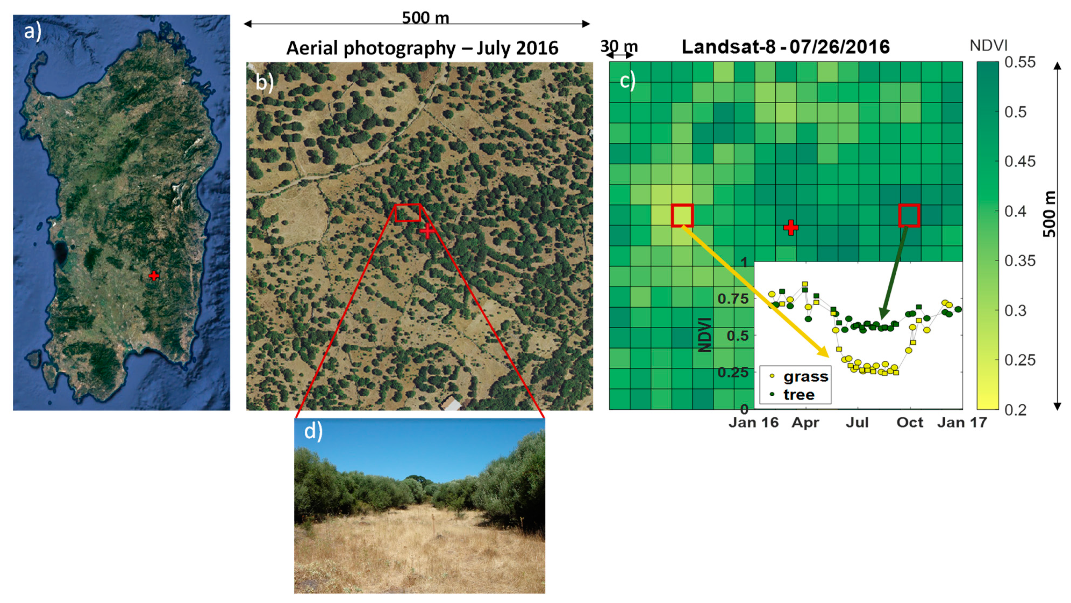
The case study and available data are first presented. Then, the proposed data assimilation approach is described.

2.1. Case Study

The proposed assimilation approach was tested with observations from a field site at Orroli, Italy, located in east-central Sardinia (39°41′12.57″N, 9°16′30.34″E, 500 m a.s.l.; [6,14,57,58]). The landscape is mainly grass (67%) and woody vegetation in the footprint area, mainly wild olives with a variable height of 3.5–4.5 m (Figure 1). The grass species grow during wet seasons and reach approximate heights of 0.5 m in spring. The soil thickness varies from 15 to 40 cm, averaging 17 ± 6 cm (standard deviation, SD) above fractured basalt [14,57]. The climate at the flux site is the maritime Mediterranean, with a mean annual precipitation of 643 mm, and a mean July precipitation of 11 mm. The mean annual air temperature (Ta) is 14.6 °C, with a mean July Ta of 23.7 °C.

2.1.1. Field Data

A 10 m micrometeorological station was operating at the site to measure land–atmosphere fluxes of energy, water, and carbon in addition to key state variables. The apparatus included a Campbell Scientific CSAT-3 sonic anemometer and a Licor-7500 CO2/H2O infrared gas analyzer positioned adjacent to each other at the top of the tower. These two instruments measured velocity, temperature, and gas concentrations for the estimation of sensible heat flux, evapotranspiration (ET), and CO2 exchanges (Fc) with the standard eddy covariance method (e.g., [59]). Half-hourly statistics were computed.
The two-dimensional footprint model of Detto et al. [6], previously tested for this site, was used for interpreting eddy correlation measurements in the context of the contributing land cover area. The combined use of the footprint model and the satellite images allowed us to interpret the eddy-covariance-observed surface flux and distinguish the source area of each vegetation component and bare soil from the measured flux, using the methodology in Detto et al. [6]. Considering the main eddy covariance tower footprint at the Sardinian site [6], an area of ~500 m × 500 m around the tower (~90% of the footprint) was considered for model predictions (Figure 1).
The surface temperature of the tree canopy and grass/bare soil patches (using IRTS-P by Apogee Instruments), incoming and outgoing shortwave and longwave radiation (from which to derive net radiation) (using CNR-1 by Kipp and Zonen), and the soil heat flux and temperature (using HFT3 REBS) at two locations close to the eddy covariance tower were monitored and half-hourly means were recorded. Precipitation was measured using a PMB2 CAE rain gauge. Seven frequency domain reflectometer probes (FDR, Campbell Scientific Model CS-616) were inserted in the soil close to the tower (3.3–5.5 m away) to estimate moisture at half-hourly intervals in the thin soil layer. Complete details of these measurements and data processing are available from Detto et al. [6], Montaldo et al. [14], and Montaldo et al. [58].
The LAI was measured indirectly through a ceptometer (Accupar model PAR-80, Decagon Devices Inc., Washington, DC, USA), which measures the PAR in the 400–700nm waveband, and estimates the LAI from these readings (details are given in the instruction manual edited by Decagon Devices Inc.). LAI measurements were performed mainly during the grass growth season [14]. Finally, specific leaf areas (LAI divided by dry biomass) of predominant grass (0.01 m2 gDM−1) and woody vegetation (0.005 m2 gDM−1) species were measured directly by weighing the dry biomass.

2.1.2. Remote Sensing Data

The Sentinel 1 radar data originated from the S1A and S1B satellites, and the level-1 ground-range-detected (GRD) data were used. The images were calibrated, noise corrected with a Lee filter (7 × 7), and resampled from 10 to 30 m spatial resolution [33]. S1A images were available from January 2015. From September 2016, S1B satellite images were also available.
Images from the Sentinel 2 radiometer were acquired at the L1C level and atmospherically corrected with the Sen2Cor tool of the Sentinel Application Platform (SNAP), or directly at the L2A level (already corrected). For Landsat 8, the L1TP product was used (it is radiometrically calibrated and orthorectified using ground control points and a digital elevation model), and the dark object subtraction (DOS) method was used for the atmospheric correction.

2.2. The Proposed Assimilation Approach

The assimilation approach includes: (1) remote sensing data, (2) the ecohydrological model, (3) the EnKF, and (4) the updating procedure of key LSM and VDM parameters (Figure 2). Below, each component of the proposed assimilation approach is described.

2.2.1. Optical Remote Sensing Data for LAI Estimate

NDVI is estimated from red and near-infrared spectral reflectance measurements of satellite remote sensors. We used mainly the Operational Land Imager (OLI) Landsat 8 data, and, secondly, the Sentinel 2 radiometer data for increasing the database. Landsat 8 has a temporal resolution of 16 days and a spatial resolution of 30 m for the optical bands, which is coarser than the resolution of Sentinel 2 data (up to 10 m; temporal resolution: up to 5 days), and both are freely available.
From Landsat 8 and Sentinel 2 data, NDVI is estimated at a 30 m spatial resolution. LAI is related to NDVI through the ΓN operator using an empirical approach (e.g., [18,60,61]):
LAI = Γ L ( NDVI ) = β 1 + β 2 NDVI β 3
where β1, β2, and β3 are coefficients for vegetation species. Note that analogous solutions should be derivable from different Γ L ( NDVI ) relationships.
The NDVI map was also used for identifying the fv,t fraction of tree cover in the field, which was estimated as NDVI/NDVImax following Detto et al. [6], with NDVImax as the maximum value of NDVI in the investigated field.

2.2.2. Radar Images for Soil Moisture Retrieval

The dielectric constant of the surface soil, which is related to soil moisture, can be detected from radar data. We used the Sentinel 1 radar in VV polarization because VV polarization is more sensitive to soil moisture [28,62] and less sensitive to vegetation compared with VH polarization [33,63]. The images were calibrated, noise-corrected, and resampled at a 30 m spatial resolution. The temporal resolution was approximately six days. Sentinel 1 images provide backscatter data in VV polarization ( σ vv 0 ).
We used the semi-empirical Dubois et al. [34] model for relating the ε dielectric constant to the backscatter signal. The Dubois et al. [34] model accounts for co-polarized backscatter only and was formulated using scatterometer data collected at six frequencies between 2.5 and 11 GHz. The validity range is ks < 2.5 (ks is the normalized RMS surface roughness), and the incidence angles were greater than 30° and were restricted to co-polarization (VV or HH). Here, only the VV empirical relationship was used:
σ vv 0 = 10 2.35 cos 3 β s e n   β 10 0.046 ε tan β ( k σ s e n 3 β ) λ 1.1 0.7
where λ is the wavelength; k is the wave number equal to 2 π/λ; σ is the surface roughness; and β is the local incident angle related to the radar beam angle and the latitude, exposition, and slope of the site. The inversion of Equation (2) estimates the dielectric constant from the VV polarized backscatter coefficient, knowing the soil surface roughness and specific radar configuration parameters (wavelength and incidence angle). While the radar configuration parameters are known, σ is undetermined. We used the approach of Montaldo et al. [33], which relates σ with NDVI through an empirical σ (NDVI) relationship, for accounting for the grass growth effect on radar signal, and which was just estimated at the Orroli field site (Figure 4b of Montaldo et al. [33]):
σ = −11.96 NDVI2 + 11.44 NDVI − 0.5982
With the objective of simplifying the parameterization of the retrieval models, the use of the σ (NDVI) of Montaldo et al. [33] allowed us to integrate vegetation effects in the roughness parameter, as previously suggested by Capodici et al. [64]. The use of Equation (3) in Equation (2) estimates ε, which is finally related to θ soil moisture through the Γθ operator [65]:
θ = Γ θ ( ε ) = ( 530 + 292 ε 5.5 ε 2 + 0.043 ε 3 ) 10 4

2.2.3. The Ecohydrological Model

The ecohydrological model is a three-component coupled land surface–vegetation dynamic model (LSM–VDM). The LSM predicts the soil water and energy balances. The VDM estimates the LAI evolution through time for two vegetation components (grass and trees), which are used by the LSM for computations of the energy exchanges between soil and vegetation. The details are given in Montaldo et al. [14] and Montaldo et al. [57]. Here, a summary of the main components is provided.

2.2.4. The Land Surface Model

The LSM predicts the dynamics of water and energy fluxes at the land surface on a half-hour time step (Figure 2). It includes three components of the land surface: bare soil, grass, and trees, representing two vegetated components. It is derived from the LSM of Montaldo and Albertson [66] and the surface temperature states are estimated through the force restore method [67]. The root zone supplies the bare soil and vegetation with soil moisture for evapotranspiration and controls the infiltration and runoff mechanisms. The base of the root zone represents the lower boundary of the LSM. Equations for surface temperature and the components of the energy balance (sensible heat flux, soil heat flux, and net radiation) are applied separately for each land cover component, so that the model predicts the energy balance distinctly for each land cover component [14] (Table 1).
The soil–water balance equation of the root zone is computed by
θ t = 1 d r z ( f b s I b s + f v , t I t + f v , g I g f b s E b s f v , t E t f v , g E g q D )
where θ is the soil moisture; drz is the root zone depth; Ibs is the infiltration rate on bare soil; It and Igr are the throughfall rates infiltrating into the soil covered by trees and grass, respectively; qD is the rate of drainage out of the bottom of the root zone; Ebs is the rate of bare soil evaporation; Et and Eg are the rates of transpiration of trees and grass, respectively; fv,g is the fraction of grass cover; and fbs is the fraction of bare soil [14].
The throughfall rate is modeled through a balance equation of the intercepted water by the canopy reservoir (a function of the LAI), which produces throughfall when the reservoir is saturated [66,67]. An infiltration excess mechanism, based on the Philip’s infiltration equation [68], was used for the infiltration. In unsaturated soil, the Clapp and Hornberger [69] relationships were used to describe the nonlinear dependencies of volumetric soil moisture and hydraulic conductivity on the matric potential. The qD rate was estimated using the unit head gradient assumption (Table 1; [11,14]).
Et and Eg were estimated distinctly using the Penman–Monteith equation (e.g., [70], p. 224) for each vegetation component. Canopy resistances, accounting for environmental stresses, were estimated using a typical Jarvis [71] approach (Table 1). The actual rate of bare soil evaporation was determined as α ( θ ) P E , where α(θ) is a rate-limiting function, estimated by the polynomial function of Parlange et al. [72], and PE is the potential evaporation estimated by the Penman equation (e.g., [70], Equations 10.15, 10.16, and 10.19). Hence, the total evapotranspiration was estimated as:
E T = f b s E b s + f v , t E t + f v , g E g
Paralleling the approach for ET estimation, a three-component approach was implemented for estimating the total net CO2 flux [57]:
F c = f v , t F c , t + f v , g F c , g + R b s
where Fc,t and Fc,g are the carbon exchange of trees and grass, respectively, and Rbs is the soil respiration. Carbon exchange rates for each PFT (i.e., Fc,t, Fc,g) were computed as the difference between photosynthesis and growth respiration (Table 2). Soil respiration was estimated as a function of the temperature (Table 2, [57,73,74,75]). The model parameters are presented in Table 3.
Table 1. Equations of drainage (qD), canopy resistance (rc) with stress functions of soil moisture (θ), air temperature (Ta) and vapor pressure deficit (VPD), sensible heat flux (H), net radiation (Rn), soil heat flux (G), and surface temperature (Ts) in the LSM. Parameters are defined in Table 3.
EquationsSource
Drainage
q D = k s ( θ θ s ) 2 b + 3
[11]
Canopy resistance
r c = r s , m i n L A I [ f 1 ( θ ) f 2 ( T a ) f 3 ( V P D ) ] 1
[69]
f 1 ( θ ) = { 0 θ θ w p θ l i m θ w p 1             i f   θ θ w p i f   θ w p < θ < θ l i m i f   θ θ l i m
f 2 ( T a ) = { 0 for T a T a , min and T a > T a , max 1 T a , o p t T a T a , o p t T a , min     for T a , min < T a < T a , o p t 1 for T a , o p t T a T a , max
f3 = 1 − ω log(VPD)
[74]
Sensible heat flux
H = ρ a c p C H u ( T s T a ) ,
where CH the heat transfer coefficient
[14]
Net radiation
R n = R s w i n ( 1 α ) + ε ( R l w i n σ T s 4 ) ,
with shortwave incoming ration, Rswin; longwave incoming ration, Rlwin, estimated based on Equation 6 in Brutsaert (1982); α—albedo; ε—emissivity; σ—the Stefan–Boltzmann constant
[14]
Soil heat flux
G = RnHLE
[14]
Surface temperature
d T s d t = C T G 2 π τ ( T s T a ) ,
where T2 is the mean Ts value over one day, τ, and CT is the soil thermal coefficient
d T 2 d t = 1 τ ( T s T 2 )
[14]
Table 2. Equations of the vegetation dynamic model components. Parameters are defined in Table 3.
Ecophysiological TermEquationsSource
Photosynthesis P h = ε P ( P A R ) f P A R P A R 1.37 r a + 1.6 r c , m i n 1.37 r a + 1.6 r c
ε P ( P A R ) = a 0 + a 1 P A R + a 2 P A R 2
f P A R = 1 e k e L A I
[76]
AllocationFor the tree cover:
a a = ξ a 1 + Ω [ 2 λ f 1 ( θ ) ]
a s = ξ s + Ω ( 1 λ ) 1 + Ω [ 2 λ f 1 ( θ ) ]
a r = ξ r + Ω ( 1 f 1 ( θ ) ) 1 + Ω [ 2 λ f 1 ( θ ) ]
ξ a + ξ s + ξ r = 1 ; λ = e k e L A I
[14]
For grass cover:
a a = ξ a + Ω λ 1 + Ω [ 1 + λ f 1 ( θ ) ]
a r = ξ r + Ω ( 1 f 1 ( θ ) ) 1 + Ω [ 1 + λ f 1 ( θ ) ]
ξ a + ξ r = 1
[14]
RespirationMaintenance and growth respirations of biomass components:
R l , μ = m a f 4 ( T ) B l ;   R l , γ = g a a a P g
R s , μ = m s f 4 ( T ) B s ;   R s , γ = g s a s P g
R r , μ = m r f 4 ( T ) B r ;   R r , γ = g r a r P g
[77]
f 4 ( T ) = Q 10 T m 10    with Tm = mean daily temperature[76]
Soil   respiration R b s = R 10 Q N T m 10
where R10 is the reference respiration rate at 10 °C and QN is the soil respiration sensitivity to temperature
[57]
Senescence S l = d a B l
S s = d s B s S r = d r B r
[14,77]
Litterfall L a = k a B d [14,77]
Table 3. Model parameters of the coupled LSM–VDM and their values for the Orroli site.
ParameterDescriptionValue
GrassTree
LSM–VDM parameters
rs,min [s m−1]Minimum stomatal resistance100300
Tmin [°K]Minimum temperature272.15272.15
Topt [°K]Optimal temperature295.15285.15
Tmax [°K]Maximum temperature313.15318.15
θwp [-]Wilting point0.080.04
θlim, [-]Limiting soil moisture for vegetation0.200.17
ω [KPa−1]Slope of the f3 relation0.60.6
Only VDM parameters
cl [m2 gDM−1]Specific leaf areas of the green biomass in growing season0.010.005
cd [m2 gDM−1]Specific leaf areas of the dead biomass0.010.003
ke [-]PAR extinction coefficient0.50.5
ξa [-]Parameter controlling allocation to leaves0.60.55
ξs [-]Parameter controlling allocation to stem-0.1
ξr [-]Parameter controlling allocation to roots0.40.35
Ω [-]Allocation parameter0.80.8
ma [d−1]Maintenance respiration coefficients for aboveground biomass0.0320.001
ga [-]Growth respiration coefficients for aboveground biomass0.280.69
mr [d−1]Maintenance respiration coefficients for root biomass0.0070.002
gr [-]Growth respiration coefficients for root biomass0.10.1
Q10 [-]Temperature coefficient in the respiration process2.452.42
da [d−1]Death rate of aboveground biomass0.050.0045
dr [d−1]Death rate of root biomass0.0030.005
ka [d−1]Rate of standing biomass pushed down0.050.35
Only LSM parameters
zom,v [m]Vegetation momentum roughness length0.050.5
zov,v [m]Vegetation water vapor roughness lengthzom/7.4zom/2.5
zom,bs [m]Bare soil momentum roughness length0.015
zov,bs [m]Bare soil water vapor roughness lengthzom/10
θs [-]Saturated soil moisture0.53
b [-]Slope of the retention curve8
ks [m/s]Saturated hydraulic conductivity5 × 10−6
|ψs| [m]Air entry suction head0.79
drz [m]Root zone depth0.19

2.2.5. The Vegetation Dynamic Model

The VDM computes the change in biomass over time from the difference between the rates of biomass production (photosynthesis) and loss, mainly respiration (e.g., [10,75]). The VDM distinguishes tree and grass components and was adapted from Montaldo et al. [76], who derived a VDM for grass species starting from the Nouvellon et al. [77] model. In the VDM of trees, four separate biomass states were considered: green leaves (Bl), stem (Bs), living root (Br), and standing dead (Bd). The VDM of grass only distinguishes three biomass states (green leaves, roots, and standing dead). The biomass [g DM m−2] components were simulated using the approach of Montaldo et al. [76], which consists of a balance between biomass production (related to photosynthesis for green leaves, stem, and roots biomass) and biomass destruction (respiration and senescence for green leaves, stem, and roots biomass), through ordinary differential equations, integrated numerically at a daily time step.
d B l d t = a a P h R l , μ R l , γ S l
d B s d t = a s P h R s , μ R s , γ S s
d B r d t = a r P h R r , μ R r , γ S r
d B d d t = S l L a
where P h is the gross photosynthesis; aa, as and ar are the allocation (partitioning) coefficients for leaves, stem, and root states, respectively; Rl,μ, Rs,μ, and Rr,μ are the maintenance respiration rates from leaves, stem, and root biomass, respectively; Rl,γ, Rs,γ, and Rr,γ are the growth respiration rates from leaves, stem, and root biomass, respectively; Sg, Ss, and Sr are the senescence rates of leaves, stem, and root biomass, respectively; La is the litterfall. The model equations are given in Table 2 and the parameters are presented in Table 3.
The leaf area index was estimated from the biomass by a linear relationship [13,76,77,78]:
LAI = c l   B l
where cl is the specific leaf area of the green biomass. The VDM provides estimates of daily values of leaf biomass and, thus, the LAI of the tree and grass was used by the LSM to estimate evapotranspiration, energy flux, rainfall interception, carbon assimilation, and the soil water content at a half-hour time step [14]. The LSM provides soil moisture and aerodynamic resistances to the VDM. The coupled model was calibrated and validated in Montaldo et al. [14] and Montaldo et al. [57]. The details are given in Montaldo et al. [76], Montaldo et al. [14], and Montaldo et al. [57].

2.2.6. The Ensemble Kalman Filter

Using the EnKF, we assimilated observations of 1) NDVI, which is related to LAI through Equation (1) in the VDM that describes the evolution of the leaf biomass through (8) that is related to LAI through (12); and 2) the radar-derived dielectric constant of the ground, which is related to θ through (4), in the LSM that describes the evolution of θ using (5). Hence, in the proposed approach, the EnKF is applied distinctly to the LSM and the VDM of both grass and tree components (Figure 2). In general, in the Kalman filters, φ is a vector of surface state variables (i.e., θ or LAI). The equation describing the evolution of these states (Equation (5) for θ and Equations (8) and (12) for LAI), as determined by a nonlinear model ( f ), can be written in general as (e.g., [79]):
d φ d t = f ( φ , ω )
where ω relates errors in model physics, parameterization, and/or forcing data, and is taken to be with mean zero and covariance Ω . H is the operator that represents the observation process that relates φ to the δ ( t j ) actual measurements available at the time, tj, as follows:
δ ( t j ) = H [ φ ( t j ) ] + ϵ ( t j )
where ϵ represents the vector of measurement errors, assuming a probabilistic distribution with a zero mean and covariance R .
In the EnKF [39,40], an ensemble of φ ζ (ζ= 1, …, Ne, with Ne the size of the ensemble) is predicted in parallel, using (13). The EnKF updates each ensemble member separately, using the δ ( t j ) observation and the diagnosed state error covariance P ( t j ) (e.g., [39], Equation (6)). The superscripts “−” and “+” refer to the state estimates before and after the update at time tj, respectively. Ensemble members are updated using a combination of forecast model states and the observations [39], as follows:
φ ζ + = φ ζ + K [ δ H ( φ ζ ) + ϵ ζ ]
where K is the Kalman gain, which depends on P ; ϵ ζ is a random realization of the measurement error, which should have the same statistical properties as the error included in (14) [80]. The mean of the ensemble members, φ ¯ + ( t j ) , is the state estimate of the variables (i.e., θ ¯ + or L A I ¯ + ).
Model errors in the EnKF are included through errors in the model initial conditions, physical parameters, and forcing data. In the assimilation of radar backscatter data in the LSM we included errors in (1) soil moisture initial conditions, (2) precipitation (whose uncertainty is expected to have significant impacts on the distribution of soil moisture, e.g., [80]), and (3) a key parameter—the saturated hydraulic conductivity (ks)—following Montaldo et al. [38]. The ensemble of soil moisture initial values is generated by altering a particular value of soil moisture through the addition of a normally distributed perturbation with a zero mean and SDθ (standard deviation). At each time step, the ensemble of precipitation is generated by multiplying the recorded precipitation value by a normally distributed random variable. An ensemble of saturated hydraulic conductivity values ( k s ζ ) is generated as being log10 normally distributed with a mean of l o g ( k ^ s ) (indicating with k ^ s the base (i.e., best guess) value of the k s ζ ensemble) and the standard deviation of SDlogks. In this way, an ensemble of θ ζ , which includes model errors, is generated and evolves in time according to (5).
We also assimilated grass and tree NDVI data in the VDM, including errors of (i) LAI initial conditions; (ii) incoming short-wave solar radiation (Rswin), and the photosynthetically active radiation (PAR); and (iii) model parameters—the maintenance respiration coefficients for the aboveground biomass (ma) of grass and trees (Table 2). We chose ma as the VDM parameter for data assimilation after a sensitivity analysis of LAI to VDM parameters, which proved the high sensitivity of grass and trees LAI to ma [56]. The ensemble of LAI initial values was generated by altering a particular value of LAI through the addition of a normally distributed perturbation with a zero mean and SDLAI standard deviation. At each time step, the ensembles of Rswin and PAR were generated by multiplying the recorded Rswin and PAR values by normally distributed random variables. The ensembles of grass and tree maintenance respiration coefficients ( m a , g ζ for grass and m a , t ζ for trees), were generated as being normally distributed with means of m ^ a , g and m ^ a , t and standard deviations of SDmag and SDmat, respectively. In this way, ensembles of LAIζ of grass and trees, which include model errors, were generated and evolved in time according to (8) and (12). The time steps of models and observations are shown in Figure 2.
The radar δ observations available at time tj,θ were obtained including the ϵ l random error in the ε observations derived from Sentinel 1 according to (14), where the operator H is the inverse of Γ θ in (4). Similarly, the NDVI observations available at time tj,L derived from Landsat 8 (or Sentinel 2) were altered randomly according to (14), where the operator H is the inverse of Γ L in (1).
When observations from Sentinel 1 are available, the ensemble of θ ζ (i.e., θ ζ ( t j , θ ) ) is replaced by (e.g., updated to) the ensemble θ ζ + ( t j , θ ) that is optimally estimated by (15) using the radar backscatter observations. When observations from Landsat 8 (or Sentinel 2) are available, the ensemble of L A I ζ (i.e., L A I ζ ( t j , L ) ) is replaced by (or updated to) the ensemble L A I ζ + ( t j , L ) , which is optimally estimated by (15) using the NDVI observations.

2.2.7. The Updating of Model Parameters through the Assimilation

The EnKF approach compensates for both inaccurate initial conditions and moderate model parameter errors. In presence of high inaccuracy of model parameters, they can be adjusted dynamically through the assimilation process. The assimilation procedure includes an update of the ks parameter of the LSM, and the grass and tree maintenance respiration coefficients of the VDM.
The ks parameter is updated using the approach of Montaldo et al. [38], based on an expression derived by Montaldo and Albertson [81], that estimates the biased error in ks from analysis of the persistent-state variable bias (as defined by a longer time average). Each component of the k s ζ ensemble is updated over an appropriate averaging time interval (Δt5; Figure 2), which coincides with time steps tξ,θ, through
k s ζ + ( t ξ , θ ) = k s ζ ( t ξ , θ ) d r z χ 1 ζ ( 2 b + 3 ) k s ζ ( t ξ , θ ) χ 2 ζ
χ 1 ζ = ( θ 2 ζ ( t j , θ ) θ s , 2 ) 2 b 2 3 [ θ 2 ζ + ( t j , θ ) θ 2 ζ ( t j , θ ) ] [ θ 2 ζ + ( t j , θ N s a ) θ 2 ζ ( t j , θ N s a ) ] Δ t 3 ¯
χ 2 ζ = θ 2 ζ + ( t j , θ ) θ 2 ζ ( t j , θ ) θ 2 ζ ( t j , θ ) ¯
where Δt3 is the radar observation time steps (Figure 2). The overbar in (17) and (18) provides an averaging in the Δt5 time steps (≥Δt3) for capturing an estimate of the “persistent” moisture bias estimating the required change in the saturated conductivity. In this way, the biased model error can be removed after a learning (calibration) period, and the Kalman filter assumption, the zero mean model error, can be recovered.
The maintenance respiration coefficient for the aboveground biomass of the VDM is updated using the approach of Montaldo and Gaspa [56] (Appendix A), which updates (i.e., dynamically adjusts) the ma based on observations of persistent bias in the modeled biomass (i.e., LAI). The proposed procedure derives the required ma adjustment from the conservation equation of the biomass (i.e., LAI), and we applied it for both grass and tree LAI. Each component of the m a , g ζ and m a , t ζ ensembles was updated over the Δt6 time interval, which coincides with time steps tξ,L (Appendix A), as follows:
m a ζ + ( t ξ , L ) = m a ζ ( t ξ , L ) ξ 1 ξ 2
ξ 1 = m a ζ ( t j , L ) LAI ζ ( t j , L ) ( LAI ζ + ( t j , L ) LAI ζ ( t j , L ) ) ¯
ξ 2 = [ LAI ζ + ( t j , L ) LAI ζ ( t j , L ) ] [ LAI ζ + ( t j , L N l a ) LAI ζ ( t j , L N l a ) ] f 3 ( t j , L ) LAI ζ ( t j , L ) Δ t 4 ¯
where Δt4 is the NDVI observation time steps (Figure 2), and the overbar in (20) and (21) provides an averaging in the Δt6 time steps (≥Δt4). In this way, an estimate of the “persistent” LAI bias is used for evaluating the necessary change in ma. Thereby, after a learning (calibration) period, the error of the model can be eliminated. We used the same solution for grass ( m a , g ζ + ) and tree ( m a , t ζ + ) maintenance respiration coefficients.

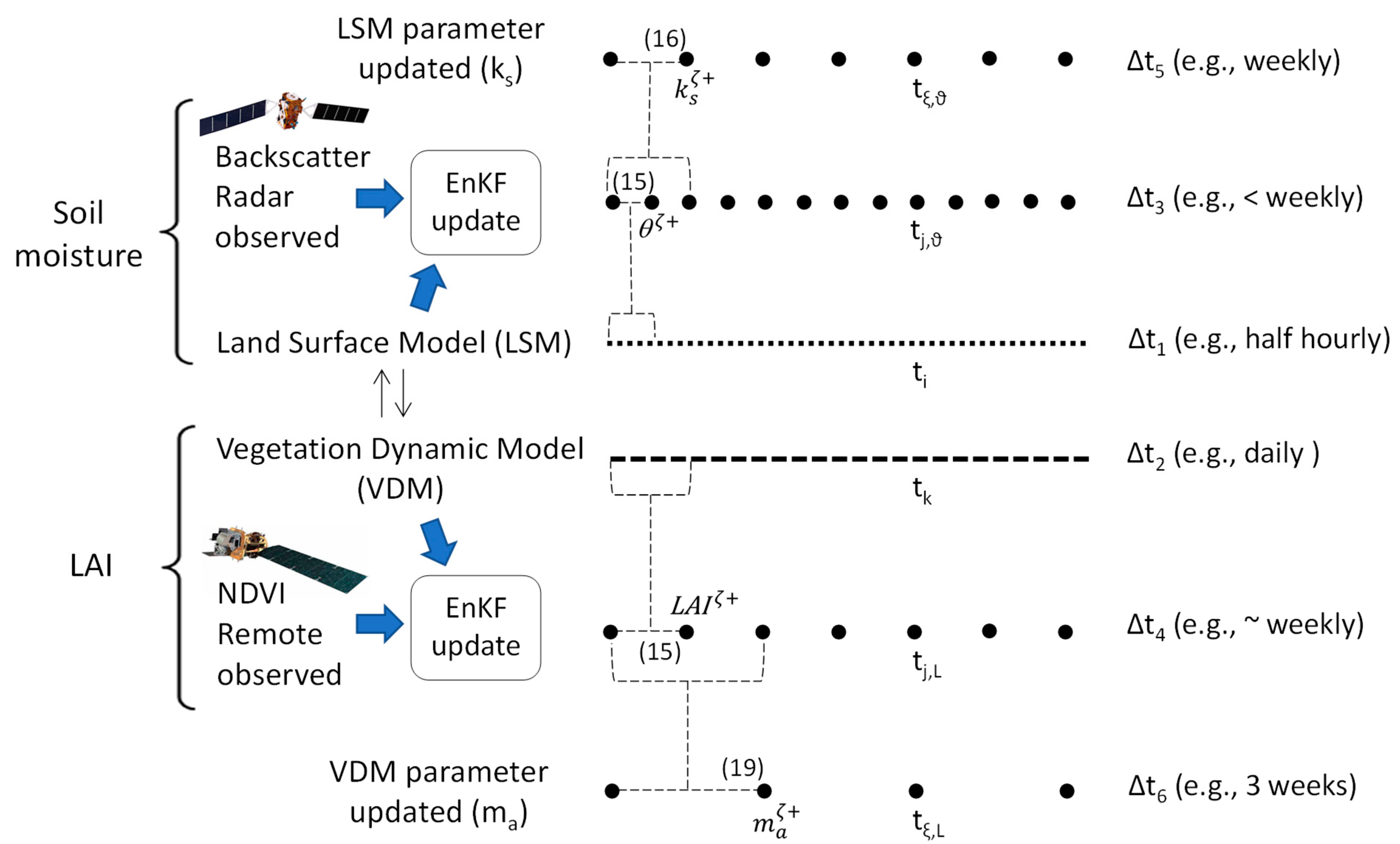
2.2.8. The Multiscale Assimilation Approach

In summary, the multiscale assimilation scheme includes the following elements (Figure 2):
  • A land surface model that predicts the ensemble of soil moisture states through (5) at the half-hourly timescale (Δt1);
  • A vegetation dynamic model that predicts the ensembles of grass and tree LAI through (8) and (12) at a daily timescale (Δt2);
  • EnKF filters of the ε observations (4), which are available every 6 days on average (Δt3); these account for moderate LSM errors and provide optimal updates of the ensemble of θ ζ ( t j ) through (15) to arrive at θ ζ + ;
  • EnKF filters of the NDVI remote data (1) of grass and trees, available over the weekly timescale on average (Δt4), which optimally update the ensembles of L A I ζ of grass and trees through (15) to arrive at L A I ζ + ;
  • An ensemble of the key LSM parameter, k s ζ , which is updated through (16) over the weekly timescale (Δt5);
  • Finally, the m a ζ ensembles of grass and trees that are updated through (19) at > weekly (e.g., 3 weeks) timescale (Δt6).
Note that the time step of k s ζ updating was lower than m a ζ updating because the dynamics of the water in the soil layer, especially in the case of thin soil layers, are faster than the slow vegetation change dynamics. Note also that the assimilation procedure of radar backscatter data (step 3) is independent to the assimilation of optical image data (step 4), so that the timing of ε observations and NDVI remote data can be different.
Hereafter, we indicate the ensemble open loop without assimilation (i.e., only steps 1 and 2) as “EnOL”. “EnKF” indicates the assimilation approach that includes the ensemble Kalman filter only (i.e., steps 1, 2, 3, and 4), and “EnKFdc” indicates the assimilation approach that includes the six steps described above.
We proved the performance of the assimilation approach for increasing the uncertainty of the model (given the observation errors) so that the proposed assimilation approach will be tested for increasing prescribed errors in ks and the grass and tree ma model parameters (compared with the calibrated values), comparing EnOL, EnKF, and EnKFdc performances.

2.2.9. Application of the Assimilation Approach to the Case Study
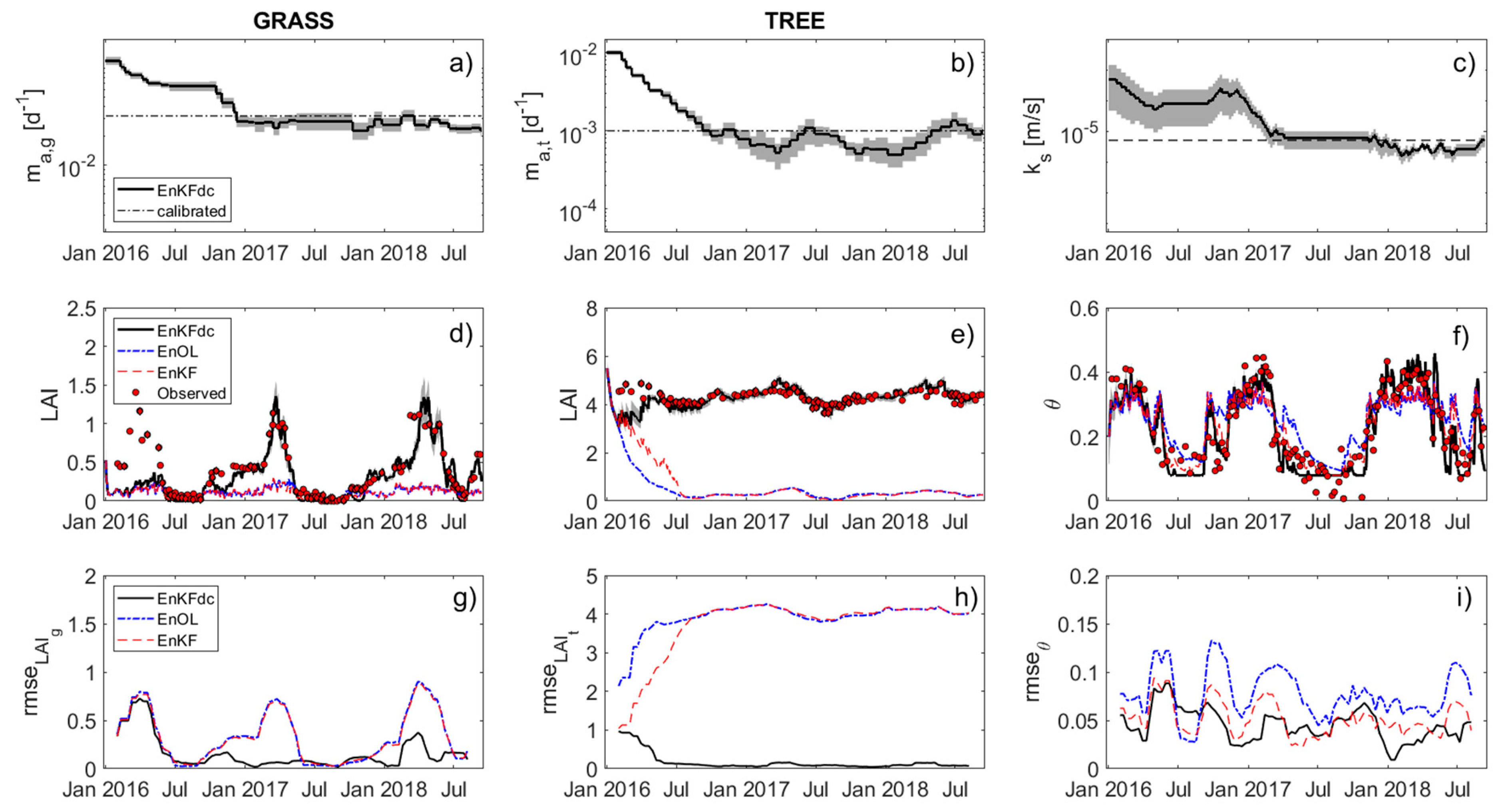
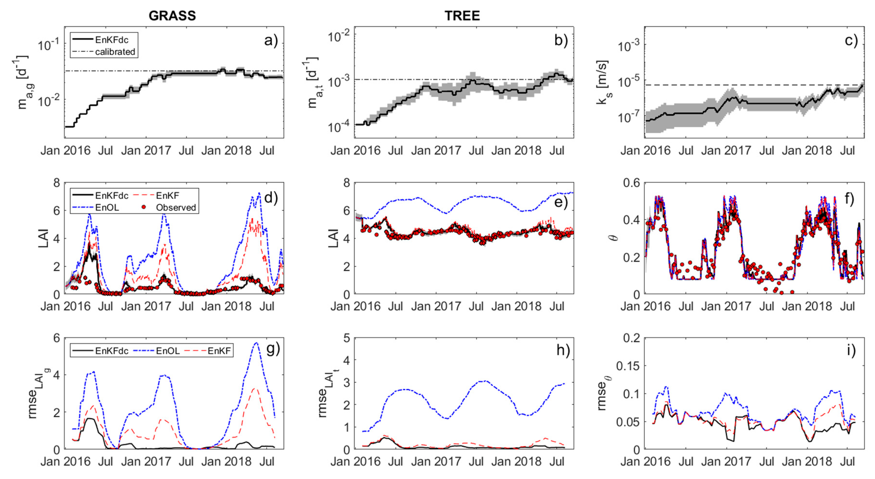
In total, Sentinel 1 data were collected for 153 days from January 2016 to August 2018, for which σ0vv backscattering coefficients were available. Data were collected, analyzed, and corrected to include the vegetation growth effect on the radar backscatter in Montaldo et al. [33], so that we used the ε time series produced by Montaldo et al. [33].
A total of 124 images of optical sensors were acquired (75 images from Landsat 8 and 49 images from Sentinel 2, see Figure 1c for the 2016–2018 period), from which the NDVI was derived at a 30 m spatial resolution. The coefficients of (1) were estimated using simultaneous NDVI data from remote sensors and LAI observations in the field (a total of 24 simultaneous days) distinguishing grass and trees (β1 = −0.435, β2 = 1.014 and β3 = 0.4029 for grass in the autumn–winter period; β1 = −0.141, β2 = 1.720, and β3 = 1.674 for grass in the spring–summer period; β1 = 0, β2 =5.392 and β3 = 0.486 for trees).
In this case study, the LSM time step was half an hour (Δt1), the VDM time step was one day (Δt2), the assimilation time step of grass and tree NDVI data (Δt4) was variable according to data availability, ranging from 2 days to 20 days with an average of 6 days, and the time step of the m a , g ζ and m a , t ζ updating was 3 weeks for both grass and trees (Δt6, Figure 2). Note that, because the VDM was applied distinctly for grass and tree in the Sardinian heterogeneous ecosystem, the grass and tree cells need to be selected in the field as representatives of the two main vegetation components for distinctly assimilating grass and tree NDVI, which were estimated in those cells in the VDM. The assimilation time step of the Sentinel 1 dielectric constant was ≤6 days (Δt3), and k s ζ was updated every 6 days (Δt5). In the EnKF, Ne was 100, which is a sufficiently large number for accurate predictions [38,39,79].
We assumed the measurement errors to be with zero mean with a standard deviation of 0.025 for both grass and tree NDVI. The measurement error ε was assumed to be a zero mean with a standard deviation of 0.1, which corresponded to an error of about 5% in the θ observations. In the VDM, we generated the ensembles of the initial LAI values for grass (LAIg) and tree (LAIt) from a Gaussian distribution with means of 0.5 and 5.5, respectively, intentionally different from the observations, and a standard deviation σ L A I of 0.2 for both grass and tree LAI. In the LSM, the ensembles of initial θ ζ were generated from a Gaussian distribution with a mean of 0.2; this was intentionally lower (20%) than the observed value, with a standard deviation of 0.05. At each time step, we generated the ensembles of the following: (i) the precipitation, by multiplying the recorded precipitation value by a normally distributed random variable with a zero mean and a standard deviation equal to 20%; (ii) the incoming solar radiation; (iii) the PAR by multiplying the measured values by a normally distributed random variable with mean zero and a standard deviation equal to 10%. It should be noted that the errors of the initial model states and parameters were uncorrelated.
The proposed assimilation approach was tested by comparing the EnOL, EnKF, and EnKFdc approaches for seven initial m a , g ζ and m a , t ζ ensembles at most, generated with seven different initial m ^ a , g and m ^ a , t values (0.0032, 0.009, 0.015, 0.032, 0.045, 0.07, and 0.12 d−1 for grass; 0.0001, 0.0003, 0.0006, 0.001, 0.004, 0.006, and 0.01 d−1 for trees) with the same SDmag and SDmat (5% of the initial value), and for five initial k s ζ at most, generated for five different initial k ^ s (5 × 10⁻⁸, 5 × 10⁻⁷, 5 × 10⁻⁶, 5 × 10⁻⁵, and 5 × 10⁻⁴ m/s) with the same SDlogks of 0.98.

3. Results

Aerial photography on a dry summer day (July 2016; Figure 1b) successfully depicts the heterogeneity of the field site—a typical Mediterranean landscape, with open areas covered in grass or bare soil depending on the season, and surrounded by trees (in this case, wild olive trees) (Figure 1a). The 30 m spatial resolution of the NDVI map estimated by the Landsat 8 image of a close day (26 July 2016; Figure 1c) was enough to identify the spatial variability of the vegetation cover (differences of 5% of the fraction of tree cover in the footprint). We identified the two representative cells of grass and tree from the NDVI map: the tree cell was the cell with the highest NDVI, while the grass cell, in which the vegetation contribution was absent in the dry summer because bare soil was predominant, was the cell with the lowest NDVI (Figure 1c). During the year, tree NDVI values were always high ranging between ~0.6 (in summer) and ~0.8 (in spring), while grass NDVI changed widely with the seasons from ~0.2 (in summer) to ~0.8 (in spring) (Figure 1c). The NDVI data of these representative cells were assimilated in the coupled LSM–VDM model as representative of the two main vegetation components.
We tested the proposed assimilation approach for the case of extremely biased model parameters. In the following, the θ, grass, and tree LAI observations are those estimated from remote sensing data (i.e., using (4) and (1), respectively). We generated initial k s ζ , m a , g ζ , and m a , t ζ ensembles with initial k ^ s , m ^ a , g , and m ^ a , t values (=5 × 10⁻⁴ m/s, 0.12 d−1, and 0.01 d−1, respectively), which were greatly higher than the corresponding calibrated values (Figure 3). The use of the EnKF was not enough for guiding the models, because grass LAI was still underpredicted during the growing seasons, similar to the results with the EnOL configuration; RMSE values were still high, up to 0.8; and observed grass LAI was higher than 1 (Figure 3d,g). The predicted tree LAI using the EnKF was even worse, with values lower than 0.3, while the observed tree LAI from remote data was around 4, and RMSE became close to 4 after 8 months of simulation when the initial model conditions were lost (Figure 3e,h). The results for θ predictions using the EnKF configuration were slightly better when compared with those using the EnOL configuration (Figure 3f,i); however, the model was still underpredicting the soil moisture during the wet months (up to 50% in autumn 2017) when the hydraulic conductivity greatly affected the soil moisture budget predictions due to the prescribed errors in ks. The EnKFdc approach dynamically calibrated the three key model parameters, which converged to values close to the calibrated values after 8–13 months (Figure 3), becoming the coupled model recalibrated for the 2017 and 2018 predictions. In 2016, the model was not yet recalibrated and the RMSE was still high, because the approach requires time for capturing and correcting the persistent model errors. Thanks to the model parameter updating, after almost one year, the RMSE of tree LAI became almost negligible (Figure 3h), and the RMSE of grass LAI decreased to values lower than 0.3 (Figure 3g). Soil moisture was better predicted using the EnKFdc configuration (Figure 3f), with values close to the radar-observed soil moisture during the wet months due to the correction of the hydraulic conductivity.
Similar supportive results were obtained generating k s ζ , m a , g ζ , and m a , t ζ ensembles with initial k ^ s , m ^ a , g , and m ^ a , t values, respectively (=5 × 10⁻⁸ m/s, 0.0032 d−1, and 0.0001 d−1, respectively). These were greatly lower than the corresponding calibrated values (Figure 4). Again, while the EnKF configuration was not enough to guide the model, the use of the EnKFdc approach updated the three model parameters, which reached values close to the corresponding calibrated values after almost one year (Figure 4a–c). Using the EnKFdc approach, the errors of grass and tree LAI predictions when compared to satellite observations were almost negligible (RMSE < 0.15 for grass LAI and RMSE < 0.1 for tree LAI in the 2017 and 2018 years; Figure 4g,h). These also decreased for the soil moisture predictions, especially during the unusually wet 2018 (Figure 4i).
For fully evaluating the proposed assimilation approach, we compared the performance of the EnKFdc, EnKF, and EnOL approaches on soil moisture and grass and tree LAI predictions for all the ranges of initial m ^ a , g , m ^ a , t , and k ^ s values, which vary independently (Figure 5 and Figure 6). For assessing the contribution of radar backscatter and NDVI assimilations separately, we compared the assimilation results in the cases of (i) assimilation of radar backscatter only; (ii) assimilation of grass and tree NDVI only; and (iii) assimilation of both radar backscatter and grass and tree NDVI (Figure 5 and Figure 6). Compared to the EnOL-based results, when radar backscatter was assimilated using the EnKF approach, the soil moisture predictions improved for the whole range of parameters (RMSE < 0.06 for most of the parameter ranges; Figure 5b). These results were improved compared with those assimilating NDVI data only, while still in the EnKF configuration (RMSE was still high, up to 0.12, for high m ^ a , g and m ^ a , t ; Figure 5c). However, the use of the EnKFdc approach further improved the model performance, which was again better when radar backscatter was assimilated. The assimilation of both radar backscatter and grass and tree NDVI enabled us to guide and correct the model for the full range of parameters, with the RMSE of soil moisture always lower than 0.045 (Figure 5g), which is a sort of minimum RMSE value due to the intrinsic errors of the model and observations themselves in soil moisture estimates.
Although the EnKF-based assimilation of NDVI only was already able to sufficiently predict the grass LAI for most parameter ranges with RMSE lower than 1.1 (Figure 6c), the use of the proposed EnKFdc approach—by assimilating both radar backscatter and NDVI—enabled us to make very good predictions of the grass LAI with RMSEs lower than 0.14 (Figure 6g). Instead, the assimilation of only radar backscatter was not enough for successfully predicting grass LAI using both EnKF and EnKFdc for m ^ a , g and m ^ a , t values lower than the calibrated values (Figure 6b,e). Similarly, the use of the proposed EnKFdc assimilation approach predicted the tree LAI well (Figure 6n), with RMSEs lower than 0.1 for the full ranges of parameter values. Instead, again, the use of only the EnKF led to a large misestimate of the tree LAI for m ^ a , g and m ^ a , t values higher than the calibrated values (Figure 6k).
The accuracy of the proposed assimilation approach when both radar backscatter and grass and tree NDVI were assimilated was tested seasonally, comparing model predictions of soil moisture and grass and tree LAI using EnOL, EnKF, and EnKFdc approaches in the four seasons for the last two investigated years and using all the combinations of initial k ^ s , m ^ a , g , and m ^ a , t values (Figure 7). The errors in the soil moisture predictions were removed partially using the EnKF in fall and summer, with a low variability range of RMSE—nearby to the mean RMSE value of ~0.06 (Figure 7a); meanwhile, errors were still high and highly variable in winter and spring (with RMSE values ranging between 0.03 and 0.06). The use of the EnKFdc removed the model bias for the soil moisture predictions in all the seasons, where the RMSE values were always coincidental with the seasonal mean RMSE values (~0.04 in winter and spring and ~0.05 in fall and summer; Figure 7a). In a similar way, in all seasons, the bias in the tree LAI predictions was only corrected using the EnKFdc, with RMSE becoming close to 0 and with negligible variability in RMSE using all parameter combinations (Figure 7b). Instead, using the EnKF approach, the bias in the grass LAI predictions was large in the spring—the key season for grass growth—when the EnKF-based approach was not able to guide the model sufficiently well and when the RMSE still reached high values of up to 2 (Figure 8c). Again, only the use of the proposed EnKFdc approach enabled us to completely remove the model bias, which decreased the RMSE values to 0.1 in spring, and showed negligible variability of RMSE values for all parameter combinations (Figure 7c). Note that the statistics of the model performance were computed for the October 2016–September 2018 period—that is, a period after the calibration period of ks, mag, and mat (e.g., Figure 3).
Finally, we evaluated the impact of the use of the proposed assimilation approach on the predictions of two main land surface fluxes— evapotranspiration (ET) and carbon exchange (Fc)—which are strictly related to soil moisture and vegetation growth. We used the eddy-covariance-based ET and Fc observations to evaluate the model. Although it improved the ET predictions when compared with the predictions using the EnOL configuration, the use of the EnKF was not enough to guide the model and predict the ET well for the full range of parameter combinations: total ET was underpredicted by up to 70% and was overpredicted by up to 10% for high and low m ^ a , g and m ^ a , t , respectively (Figure 8b). The use of the proposed EnKFdc allowed us to remove the model bias, and the ET was accurately predicted for the full range of the parameters (misprediction of the total ET was lower than 4%, see Figure 8c).
Similar results were obtained for Fc predictions. Indeed, the use of the EnKF approach did not remove the model bias in Fc predictions when extremely high and low m ^ a , g and m ^ a , t values were initially assumed: underprediction and overprediction of the total observed Fc occurred by up to 80% and 70%, respectively (Figure 8e). The dynamic calibration of the key model parameters using the EnKFdc approach allowed us to remove the model bias and predict the Fc well for the full ranges of parameters (misprediction of the total Fc was lower than 15%, see Figure 8f).

4. Discussion

The hydrologic database for the Sardinian site, covering almost 3 years, was very useful for testing the proposed assimilation approach, due to the wide range of hydrometeorological conditions [33], involving an extremely dry 2017 (the soil dried earlier than normal in March, with total precipitation of just 6.9 mm from March to August, see Figure 3) and a wet 2018 (soil dried shortly in July only, with total precipitation of 167.9 mm from March to August, see Figure 3).
The Sardinian field is heterogeneous, with the common Mediterranean tree species wild olives [82,83,84] randomly arranged in space (Figure 1). Although the tree cover size of these tree species was reduced, the freely available Landsat 8 and Sentinel 2 products captured the spatial variability of the NDVI and tree cover in the field (Figure 1). Montaldo et al. [33] demonstrated that the Sentinel 1 satellite can be used for reliable estimates of the soil moisture in the Sardinian site thanks to its fine spatial scale (up to 10 m), as has been shown in other Mediterranean ecosystems [85,86,87]. We demonstrated that the availability of such satellite observations at adequate high spatial and time resolutions allows to monitor the main land surface variables in heterogeneous fields. Furthermore, we have showed that they can be used for guiding ecohydrological modeling, enabling researcher to reach the final objective of an operative data assimilation approach. The proposed data assimilation approach includes the assimilation of both radar backscatter data and NDVI optical data. In this context, Pan et al. [47] and Zhuo et al. [48] assimilated radar Sentinel 1 and optical Sentinel 2 data in the WOFOST model using the EnKF for agricultural land at fine spatial resolution (10–30 m). We demonstrated that both tree and grass NDVI can be assimilated for tree and grass LAI predictions in a heterogeneous field.
The proposed multiscale assimilation approach also includes the dynamic updating through assimilation of three key model parameters—saturated hydraulic conductivity, which is mainly related to soil moisture; and the tree and grass maintenance respiration coefficients, which are mainly related to tree and grass LAI. Montaldo et al. [38], using field measurements as a proxy for remote sensor observations, highlighted the limits of the EnKF model for soil moisture prediction, especially when the key model parameters largely differ from the calibrated values. This is a typical problem of operational data assimilation approaches, which are often used in case studies with limited knowledge of model parameters and field properties [88,89]. The dynamic updating of the model parameters occurs at timescales which are longer than the LSM–VDM timescales, as proposed by Montaldo et al. [38], to capture the persistent bias in soil and biomass budget predictions. Our analysis showed that EnKF-based assimilation performed sufficiently well when the parameters were moderately different from the calibrated values both for soil moisture and for LAI predictions; meanwhile, its performance decreased when the parameters largely diverged from the calibrated values, especially for soil moisture and tree LAI predictions (Figure 5 and Figure 6). EnKF performed sufficiently well for the grass LAI predictions; although, the use of the EnKFdc approach still improved the model’s performance for the low initial values of the maintenance respiration coefficients (Figure 6).
The proposed EnKFdc approach performed well for the full range of parameters and hydrometeorological conditions. The EnKF approach was not enough to guide the models when the key parameters were largely biased, because when, for instance, the saturated hydraulic conductivity is largely over- or underestimated, the root zone soil moisture balance is not systematically preserved, and only the progressive and systematic correction of the key soil parameter—the saturated hydraulic conductivity—can correct and guide the model. Lu et al. [52,53] and Nie et al. [50] demonstrated the efficacy of a multiscale assimilation approach for soil moisture predictions with the dynamic calibration of soil parameters. Here, we included the assimilation of NDVI data through calibrating the main VDM model parameters, i.e., the maintenance respiration coefficients. The dynamic calibration of the ma parameters can guide the VDM, preserving the biomass balance of grass and tree species. The proposed EnKFdc approach for both LSM and VDM was the only approach to predict not only the soil moisture and the tree and grass LAI well, but was also the only approach to predict the main outputs of the coupled model, the evapotranspiration, and the carbon exchanges (Figure 8), which are strictly related to soil moisture and vegetation dynamics [57,90]. The use of the EnKF alone was not enough to obtain good predictions of the two key land surface fluxes, with errors up 70% in ET predictions, when lower ma values were prescribed; furthermore, the errors were up to 120% in Fc predictions when high initial ma values were prescribed. Such high model bias in ET predictions affects soil–water balance predictions in these semiarid ecosystems because ET is the main loss term of the soil water budget, with a yearly magnitude that may be equal to the precipitation [6,91,92]. ET and Fc predictions were good for the full range of model parameters when the proposed EnKFdc approach was used, showing the high performance of the approach (errors less than 4% and 15% in ET and Fc predictions, respectively).
In terms of the importance of the proposed assimilation approach in relation to the seasons, the EnKFdc approach is essential for tree LAI predictions in all the seasons because the tree LAI values of the evergreen tree species are almost constant during the year, and NDVI assimilation is important for the whole year. For grass LAI predictions, the EnKFdc approach is more important in the growing season, when grass achieved maximum height, impacting evapotranspiration and carbon exchanges [14]. The EnKFdc approach becomes even more crucial for soil moisture predictions in spring and winter, when soil is wetter, and the root zone soil budget is controlled by a key soil parameter— saturated hydraulic conductivity [93]. Winter and spring are crucial seasons for water resources management in semiarid Mediterranean ecosystems, when soil moisture and ET need to be adequately predicted due to their key roles in water resources.

5. Conclusions

This paper proposes a multiscale assimilation approach that assimilates both radar backscatter data and grass and tree NDVI data from remote sensors for guiding the predictions of soil moisture and LAI of coupled vegetation dynamic and land surface models. It is suitable for heterogeneous ecosystems, which are typical of semiarid climates, thanks to the sufficiently high spatial (10–30 m) and temporal (~weekly) resolutions of the observations of the Sentinel 1 radar, the Landsat 8 satellite, and the Sentinel 2 satellite. The assimilation approach which is based on the ensemble Kalman filter (EnKF) was not sufficient for guiding soil moisture and LAI predictions when the model was largely biased due to the values of three key model parameters—the saturated hydraulic conductivity and the grass and tree maintenance respiration coefficients—being largely different from the calibrated values. The proposed multiscale assimilation approach is not limited to assimilating remote sensing data for model predictions using the EnKF: it uses assimilated data for dynamically updating key model parameters (the ENKFdc approach) at a longer timescale. These key model parameters are the saturated hydraulic conductivity and the grass and tree maintenance respiration coefficients, which are highly sensitive parameters of soil–water balance and biomass budget models, respectively. The use of the proposed EnKFdc approach was essential for soil moisture and grass LAI predictions, especially in the winter and spring seasons, which are key seasons for the water resources management of Mediterranean semiarid ecosystems. We demonstrated that the use of the proposed assimilation approach enabled us to predict key land surface fluxes, drastically reducing model prediction errors when parameters are wrongly estimated. From these results, we can also anticipate that the proposed assimilation approach may be even more important in ecosystems under wetter climates, where the model bias effects can be even larger on a soil water budget due to misestimates of hydraulic conductivity.

Author Contributions

Conceptualization and methodology, N.M.; software, N.M., A.G. and R.C.; validation, A.G., R.C. and N.M.; data curation, A.G. and R.C.; writing—original draft preparation, N.M. and A.G.; writing—review and editing, N.M.; supervision, N.M.; project administration, N.M.; funding acquisition, N.M. All authors have read and agreed to the published version of the manuscript.

Funding

This research was funded by Italian Ministry of Education, University and Research (MIUR) through the SWATCH European project of the PRIMA MED program, CUP n. F24D19000010006, and the FLUXMED European project of the WATER JPI program, CUP n. F24D19000030001.

Data Availability Statement

The data presented in this study are openly available in zenodo.org repository at http://doi.org/10.5281/zenodo.4972597 (accessed on 1 April 2020). Sentinel-2 data are available at https://scihub.copernicus.eu/dhus/#/home (accessed on 1 April 2020), while Landsat 8 data are available at https://earthexplorer.usgs.gov/, accessed on 1 April 2020.

Acknowledgments

The authors would like to thank Copernicus Open Access Hub for providing Sentinel-1 and Sentinel-2 data, and U.S. Geological Survey Earth Explores for providing Landsat 8 data.

Conflicts of Interest

The authors declare no conflict of interest.

Appendix A

The assimilation method updates ma based on observations of persistent bias in the modeled biomass (i.e., LAI). Substituting (12) in (8), the biomass balance for the modeled “m” state variables is:
1 c l L A I m t = a a P h m R l , μ m R l , γ m S l m
Since the biomass balance must be conserved in both the model and reality, we write Equation (A1) for the observed “o” state variables.
1 c l L A I o t = a a P h o R l , μ o R l , γ o S l o
Assuming that P h m P h o , R l , γ m R l , γ o , and S l m S l o , and subtracting Equation (A2) from Equation (A1),
1 c l ( L A I o t L A I m t ) = 1 c l ( Δ L A I o , m ) t = R l , μ m R l , μ o
where Δ L A I o , m is the assimilation correction. From the maintenance respiration equation (Table 2) and Equation (12):
R l , μ m = R l , μ ( L A I m ) = m a m   f 3 ( T ) m   B l m = m a m   f 3 ( T ) m c l   L A I m
R l , μ o = R l , μ ( L A I o ) = m a o   f 3 ( T ) o c l   L A I o
assuming that f 3 m ( T ) f 3 o ( T ) , the first-order Taylor series expansion of the maintenance respiration function, concerning the modeled parameter values, connects the modeled maintenance respiration to the “real” maintenance respiration. This is in terms of differences between the modeled and “real” LAI and maintenance coefficient values, as follows:
R l , μ ( L A I o , m a o ) = R l , μ ( L A I m , m a m ) + R l , μ m a   Δ m a o , m + R l , μ L A I   Δ L A I o , m
where
Δ m a o , m = m a o m a m
Substituting Equation (A6) into (A3) relates the difference between the “real” and modeled LAI to the difference between the “real” and modeled maintenance coefficient values, as follows:
( Δ L A I o , m ) t = c l ( R l , μ m a   Δ m a o , m + R l , μ L A I   Δ L A I o , m )
Differentiating Equation (A4) and substituting into Equation (A8) yields
( Δ L A I o , m ) t = c l [ f 3 ( T ) c l   L A I m   Δ m a o , m f 3 ( T ) c l   m a m   Δ L A I o , m ]
Solving Equation (A9) for the “real” maintenance respiration coefficient, in terms of known quantities, as follows:
m a o = m a m m a m L A I m Δ L A I o , m 1 f 3 ( T ) L A I m   ( Δ L A I o , m ) t
This expression would, theoretically, provide an estimate of the actual ma at each time the LAI is updated through NDVI, from knowledge of the change in Δ L A I o , m since the last update. By averaging Equation (A10) over an appropriate time interval (Δt6, e.g., 3 weeks, Figure 2) to capture a reliable estimate of the “persistent” LAI bias, the required change in the maintenance respiration coefficient can be estimated with
m a o = m a m m a m L A I m Δ L A I o , m ¯ 1 f 3 ( T ) L A I m   ( Δ L A I o , m ) t ¯
where the overbar denotes a time-averaged term. This method is presented in Montaldo and Gaspa [56].

References

  1. Huang, S.; Ding, J.L.; Zou, J.; Liu, B.H.; Zhang, J.Y.; Chen, W.Q. Soil Moisture Retrival Based on Sentinel-1 Imagery under Sparse Vegetation Coverage. Sensors 2019, 19, 589. [Google Scholar] [CrossRef] [PubMed] [Green Version]
  2. Santi, E.; Paloscia, S.; Pettinato, S.; Brocca, L.; Ciabatta, L.; Entekhabi, D. On the synergy of SMAP, AMSR2 AND SENTINEL-1 for retrieving soil moisture. Int. J. Appl. Earth Obs. Geoinf. 2018, 65, 114–123. [Google Scholar] [CrossRef]
  3. Attarzadeh, R.; Amini, J. Towards an object-based multi-scale soil moisture product using coupled Sentinel-1 and Sentinel-2 data. Remote Sens. Lett. 2019, 10, 619–628. [Google Scholar] [CrossRef]
  4. Hill, T.C.; Quaife, T.; Williams, M. A data assimilation method for using low-resolution Earth observation data in heterogeneous ecosystems. J. Geophys. Res. 2011, 116, D08117. [Google Scholar] [CrossRef] [Green Version]
  5. Montaldo, N.; Corona, R.; Curreli, M.; Sirigu, S.; Piroddi, L.; Oren, R. Rock water as a key resource for patchy ecosystems on shallow soils: Digging deep tree clumps subsidize surrounding surficial grass. Earth’s Future 2021, 9, e2020EF001870. [Google Scholar] [CrossRef]
  6. Detto, M.; Montaldo, N.; Albertson, J.D.; Mancini, M.; Katul, G. Soil moisture and vegetation controls on evapotranspiration in a heterogeneous Mediterranean ecosystem on Sardinia, Italy. Water Resour. Res. 2006, 42, 16. [Google Scholar] [CrossRef]
  7. Axelsson, C.R.; Hanan, N.P. Patterns in woody vegetation structure across African savannas. Biogeosciences 2017, 14, 3239–3252. [Google Scholar] [CrossRef] [Green Version]
  8. Bao, Y.S.; Lin, L.B.; Wu, S.Y.; Deng, K.A.K.; Petropoulos, G.P. Surface soil moisture retrievals over partially vegetated areas from the synergy of Sentinel-1 and Landsat 8 data using a modified water-cloud model. Int. J. Appl. Earth Obs. Geoinf. 2018, 72, 76–85. [Google Scholar] [CrossRef]
  9. Ngadze, F.; Mpakairi, K.S.; Kavhu, B.; Ndaimani, H.; Maremba, M.S. Exploring the utility of Sentinel-2 MSI and Landsat 8 OLI in burned area mapping for a heterogeneous savannah landscape. PLoS ONE 2020, 15, e0232962. [Google Scholar] [CrossRef]
  10. Cayrol, P.; Chehbouni, A.; Kergoat, L.; Dedieu, G.; Mordelet, P.; Nouvellon, Y. Grassland modeling and monitoring with SPOT-4 VEGETATION instrument during the 1997–1999 SALSA experiment. Agric. For. Meteorol. 2000, 105, 91–115. [Google Scholar] [CrossRef]
  11. Albertson, J.D.; Kiely, G. On the structure of soil moisture time series in the context of Land Surface Models. J. Hydrol. 2001, 243, 101–119. [Google Scholar] [CrossRef]
  12. Montaldo, N.; Albertson, J.D.; Mancini, M.; Kiely, G. Robust simulation of root zone soil moisture with assimilation of surface soil moisture data. Water Resour. Res. 2001, 37, 2889–2900. [Google Scholar] [CrossRef] [Green Version]
  13. Arora, V.K. Simulating energy and carbon fluxes over winter wheat using coupled land surface and terrestrial ecosystem models. Agr. For. Meteorol. 2003, 118, 21–47. [Google Scholar] [CrossRef]
  14. Montaldo, N.; Albertson, J.D.; Mancini, M. Vegetation dynamics and soil water balance in a water-limited Mediterranean ecosystem on Sardinia, Italy. Hydrol. Earth Syst. Sci. 2008, 12, 1257–1271. [Google Scholar] [CrossRef] [Green Version]
  15. Baghdadi, N.; El Hajj, M.; Zribi, M.; Bousbih, S. Calibration of the Water Cloud Model at C-Band for Winter Crop Fields and Grasslands. Remote Sens. 2017, 9, 969. [Google Scholar] [CrossRef] [Green Version]
  16. Bousbih, S.; Zribi, M.; El Hajj, M.; Baghdadi, N.; Lili-Chabaane, Z.; Gao, Q.; Fanise, P. Soil moisture and irrigation mapping in A semi-arid region, based on the synergetic use of Sentinel-1 and Sentinel-2 data. Remote Sens. 2018, 10, 1953. [Google Scholar] [CrossRef] [Green Version]
  17. Urban, M.; Berger, C.; Mudau, T.E.; Heckel, K.; Truckenbrodt, J.; Odipo, V.O.; Smit, I.P.J.; Schmullius, C. Surface Moisture and Vegetation Cover Analysis for Drought Monitoring in the Southern Kruger National Park Using Sentinel-1, Sentinel-2, and Landsat-8. Remote Sens. 2018, 10, 1482. [Google Scholar] [CrossRef] [Green Version]
  18. Wang, Q.; Adiku, S.; Tenhunen, J.; Granier, A. On the relationship of NDVI with leaf area index in a deciduous forest site. Remote Sens. Environ. 2005, 94, 244–255. [Google Scholar] [CrossRef]
  19. Verrelst, J.; Camp-Valls, G.; Muñoz-Marí, J.; Rivera, J.P.; Veroustraete, F.; Clevers, J.G.P.W.; Moreno, J. Optical remote sensing and the retrieval of terrestrial vegetation bio-geophysical properties-A review. ISPRS J. Photogramm. Remote Sens. 2015, 108, 273–290. [Google Scholar] [CrossRef]
  20. Li, X.; Mao, F.; Du, H.; Zhou, G.; Xu, X.; Han, N.; Sun, S.; Gao, G.; Chen, L. Assimilating leaf area index of three typical types of subtropical forest in China from MODIS time series data based on the integrated ensemble Kalman filter and PROSAIL model. ISPRS J. Photogramm. Remote Sens. 2017, 126, 68–78. [Google Scholar] [CrossRef]
  21. Dong, T.; Liu, J.; Shang, J.; Qian, B.; Ma, B.; Kovacs, J.M.; Walters, D.; Jiao, X.; Geng, X.; Shi, Y. Assessment of red-edge vegetation indices for crop leaf area index estimation. Remote Sens. Environ. 2019, 222, 133–143. [Google Scholar] [CrossRef]
  22. Altese, E.; Bolognani, O.; Mancini, M.; Troch, P.A. Retrieving soil moisture over bare soil from ERS 1 synthetic aperture radar data: Sensitivity analysis based on a theoretical surface scattering model and field data. Water Resour. Res. 1996, 32, 653–661. [Google Scholar] [CrossRef]
  23. Das, N.N.; Entekhabi, D.; Dunbar, R.S.; Chaubell, M.J.; Colliander, A.; Yueh, S.; Jagdhuber, T.; Chen, F.; Crow, W.; O’Neill, P.E.; et al. The SMAP and Copernicus Sentinel 1A/B microwave active-passive high resolution surface soil moisture product. Remote Sens. Environ. 2019, 233, 17. [Google Scholar] [CrossRef]
  24. Brocca, L.; Morbidelli, R.; Melone, F.; Moramarco, T. Soil moisture spatial variability in experimental areas of central Italy. J. Hydrol. 2007, 333, 356–373. [Google Scholar] [CrossRef]
  25. Merheb, M.; Moussa, R.; Abdallah, C.; Colin, F.; Perrin, C.; Baghdadi, N. Hydrological response characteristics of Mediterranean catchments at different time scales: A meta-analysis. Hydrol. Sci. J. 2016, 61, 2520–2539. [Google Scholar] [CrossRef] [Green Version]
  26. Prakash, R.; Singh, D.; Pathak, N.P. A Fusion Approach to Retrieve Soil Moisture with SAR and Optical Data. IEEE J. Sel. Top. Appl. Earth Obs. Remote Sens. 2012, 5, 196–206. [Google Scholar] [CrossRef]
  27. Shi, J.; Du, Y.; Du, J.; Jiang, L.; Chai, L.; Mao, K.; Xu, P.; Ni, W.; Xiong, C.; Liu, Q.; et al. Progresses on microwave remote sensing of land surface parameters. Sci. China Earth Sci. 2012, 55, 1052–1078. [Google Scholar] [CrossRef]
  28. Bousbih, S.; Zribi, M.; Lili-Chabaane, Z.; Baghdadi, N.; El Hajj, M.; Gao, Q.; Mougenot, B. Potential of Sentinel-1 Radar Data for the Assessment of Soil and Cereal Cover Parameters. Sensors 2017, 17, 2617. [Google Scholar] [CrossRef] [Green Version]
  29. Chen, L.; Xing, M.; He, B.; Wang, J.; Shang, J.; Huang, X.; Xu, M. Estimating Soil Moisture over Winter Wheat Fields during Growing Season Using RADARSAT-2 Data. Remote Sens. 2022, 14, 2232. [Google Scholar] [CrossRef]
  30. Attema, E.P.W.; Ulaby, F.T. Vegetation modeled as water cloud. Radio Sci. 1978, 13, 357–364. [Google Scholar] [CrossRef]
  31. Kornelsen, K.C.; Coulibaly, P. Advances in soil moisture retrieval from synthetic aperture radar and hydrological applications. J. Hydrol. 2013, 476, 460–489. [Google Scholar] [CrossRef]
  32. El Hajj, M.; Baghdadi, N.; Zribi, M.; Belaud, G.; Cheviron, B.; Courault, D.; Charron, F. Soil moisture retrieval over irrigated grassland using X-band SAR data. Remote Sens. Environ. 2016, 176, 202–218. [Google Scholar] [CrossRef] [Green Version]
  33. Montaldo, N.; Fois, L.; Corona, R. Soil Moisture Estimates in a Grass Field Using Sentinel-1 Radar Data and an Assimilation Approach. Remote Sens. 2021, 13, 3293. [Google Scholar] [CrossRef]
  34. Dubois, P.C.; Vanzyl, J.; Engman, T. Measuring Soil-Moisture with Imaging Radars. IEEE Trans. Geosci. Remote Sens. 1995, 33, 915–926. [Google Scholar] [CrossRef] [Green Version]
  35. Wigneron, J.P.; Olioso, A.; Calvet, J.C.; Bertuzzi, P. Estimating root zone soil moisture from surface soil moisture data and soil-vegetation-atmosphere transfer modeling. Water Resour. Res. 1999, 35, 3735–3745. [Google Scholar] [CrossRef]
  36. Hoeben, R.; Troch, P.A. Assimilation of active microwave observation data for soil moisture profile estimation. Water Resour. Res. 2000, 36, 2805–2819. [Google Scholar] [CrossRef] [Green Version]
  37. Walker, J.P.; Willgoose, G.R.; Kalma, J.D. One-dimensional soil moisture profile retrieval by assimilation of near-surface observations: A comparison of retrieval algorithms. Adv. Water Resour. 2001, 24, 631–650. [Google Scholar] [CrossRef] [Green Version]
  38. Montaldo, N.; Albertson, J.D.; Mancini, M. Dynamic calibration with an ensemble kalman filter based data assimilation approach for root-zone moisture predictions. J. Hydrometeorol. 2007, 8, 910–921. [Google Scholar] [CrossRef]
  39. Reichle, R.H.; Walker, J.P.; Koster, R.D.; Houser, P.R. Extended versus ensemble Kalman filtering for land data assimilation. J. Hydrometeorol. 2002, 3, 728–740. [Google Scholar] [CrossRef]
  40. Evensen, G. Sequential Data Assimilation with A Nonlinear Quasi-Geostrophic Model Using Monte-Carlo Methods To Forecast Error Statistics. J. Geophys. Res.Ocean. 1994, 99, 10143–10162. [Google Scholar] [CrossRef]
  41. Dunne, S.; Entekhabi, D. An ensemble-based reanalysis approach to land data assimilation. Water Resour. Res. 2005, 41, 18. [Google Scholar] [CrossRef] [Green Version]
  42. Kumar, S.V.; Mocko, M.D.; Wang, S.; Peters-Lidard, C.D.; Borak, J. Assimilation of remotely sensed leaf area index into the Noah-MP land surface model: Impacts on water and carbon fluxes and states over the continental United States. J. Hydrometeorol. 2019, 20, 1359–1377. [Google Scholar] [CrossRef]
  43. Ling, X.L.; Fu, C.B.; Yang, Z.L.; Guo, W.D. Comparison of different sequential assimilation algorithms for satellite-derived leaf area index using the Data Assimilation Research Testbed (version Lanai). Geosci. Model Dev. 2019, 12, 3119–3133. [Google Scholar] [CrossRef] [Green Version]
  44. Albergel, C.; Zheng, Y.; Bonan, B.; Dutra, E.; Rodríguez-Fernández, N.; Munier, S.; Calvet, J.C. Data assimilation for continuous global assessment of severe conditions over terrestrial surfaces. Hydrol. Earth Syst. Sci. 2020, 24, 4291–4316. [Google Scholar] [CrossRef]
  45. Bonan, B.; Albergel, C.; Zheng, Y.; Barbu, A.L.; Fairbairn, D.; Munier, S.; Calvet, J.C. An ensemble square root filter for the joint assimilation of surface soil moisture and leaf area index within the Land Data Assimilation System LDAS-Monde: Application over the Euro-Mediterranean region. Hydrol. Earth Syst. Sci. 2020, 24, 325–347. [Google Scholar] [CrossRef] [Green Version]
  46. Rahman, A.; Maggioni, V.; Zhang, X.; Houser, P.; Sauer, T.; Mocko, D.M. The Joint Assimilation of Remotely Sensed Leaf Area Index and Surface Soil Moisture into a Land Surface Model. Remote Sens. 2022, 14, 437. [Google Scholar] [CrossRef]
  47. Pan, H.Z.; Chen, Z.X.; de Wit, A.; Ren, J.Q. Joint Assimilation of Leaf Area Index and Soil Moisture from Sentinel-1 and Sentinel-2 Data into the WOFOST Model for Winter Wheat Yield Estimation. Sensors 2019, 19, 3161. [Google Scholar] [CrossRef] [Green Version]
  48. Zhuo, W.; Huang, J.X.; Li, L.; Zhang, X.D.; Ma, H.Y.; Gao, X.R.; Huang, H.; Xu, B.D.; Xiao, X.M. Assimilating Soil Moisture Retrieved from Sentinel-1 and Sentinel-2 Data into WOFOST Model to Improve Winter Wheat Yield Estimation. Remote Sens. 2019, 11, 1618. [Google Scholar] [CrossRef] [Green Version]
  49. Moradkhani, H.; Sorooshian, S.; Gupta, H.V.; Houser, P.R. Dual state-parameter estimation of hydrological models using ensemble Kalman filter. Adv. Water Resour. 2005, 28, 135–147. [Google Scholar] [CrossRef] [Green Version]
  50. Nie, S.; Zhu, J.; Luo, Y. Simultaneous estimation of land surface scheme states and parameters using the ensemble Kalman filter: Identical twin experiments. Hydrol. Earth Syst. Sci. 2011, 15, 2437–2457. [Google Scholar] [CrossRef] [Green Version]
  51. Zhang, H.; Hendricks Franssen, H.J.; Han, X.; Vrugt, J.A.; Vereecken, H. State and parameter estimation of two land surface models using the ensemble Kalman filter and the particle filter. Hydrol. Earth Syst. Sci. 2017, 21, 4927–4958. [Google Scholar] [CrossRef] [Green Version]
  52. Lü, H.; Yu, Z.; Horton, R.; Zhu, Y.; Wang, Z.; Hao, Z.; Xiang, L. Multi-scale assimilation of root zone soil water predictions. Hydrol. Processes 2011, 25, 3158–3172. [Google Scholar] [CrossRef]
  53. Lü, H.; Yu, Z.; Zhu, Y.; Drake, S.; Hao, Z.; Sudicky, E.A. Dual state-parameter estimation of root zone soil moisture by optimal parameter estimation and extended Kalman filter data assimilation. Adv. Water Resour. 2011, 34, 395–406. [Google Scholar] [CrossRef]
  54. Schaap, M.G.; Leij, F.J. Improved prediction of unsaturated hydraulic conductivity with the Mualem-van Genuchten model. Soil Sci. Soc. Am. J. 2000, 64, 843–851. [Google Scholar] [CrossRef] [Green Version]
  55. Montaldo, N.; Mancini, M.; Rosso, R. Flood hydrograph attenuation induced by a reservoir system: Analysis with a distributed rainfall-runoff model. Hydrol. Processes 2004, 18, 545–563. [Google Scholar] [CrossRef]
  56. Montaldo, N.; Gaspa, A. Multi Scale Assimilation of NDVI data for Leaf Area Index Predictions in an Heterogeneous Mediterranean Ecosystem. Agric. For. Meteorol. 2022; submitted. [Google Scholar]
  57. Montaldo, N.; Corona, R.; Albertson, J.D. On the separate effects of soil and land cover on Mediterranean ecohydrology: Two contrasting case studies in Sardinia, Italy. Water Resour. Res. 2013, 49, 1123–1136. [Google Scholar] [CrossRef]
  58. Montaldo, N.; Curreli, M.; Corona, R.; Oren, R. Fixed and variable components of evapotranspiration in a Mediterranean wild-olive-grass landscape mosaic. Agric. For. Meteorol. 2020, 280, 107769. [Google Scholar] [CrossRef]
  59. Baldocchi, D.D. Assessing the eddy covariance technique for evaluating carbon dioxide exchange rates of ecosystems: Past, present and future. Glob. Change Biol. 2003, 9, 479–492. [Google Scholar] [CrossRef] [Green Version]
  60. Gupta, R.K.; Prasad, T.S.; Vijayan, D. Relationship between LAI and NDVI for IRS LISS and Landsat TM bands. Adv. Space Res. 2000, 26, 1047–1050. [Google Scholar] [CrossRef]
  61. Potithep, S.; Nasahara, N.K.; Muraoka, H.; Nagai, S.; Suzuki, R. What is the actual relationship between LAI and VI in a deciduous broadleaf forest. Int. Arch. Photogramm. Remote Sens. Spat. Inf. Sci. 2010, 38, 609–614. [Google Scholar]
  62. Amazirh, A.; Merlin, O.; Er-Raki, S.; Gao, Q.; Rivalland, V.; Malbeteau, Y.; Khabba, S.; Escorihuela, M.J. Retrieving surface soil moisture at high spatio-temporal resolution from a synergy between Sentinel-1 radar and Landsat thermal data: A study case over bare soil. Remote Sens. Environ. 2018, 211, 321–337. [Google Scholar] [CrossRef]
  63. Dabrowska-Zielinska, K.; Musial, J.; Malinska, A.; Budzynska, M.; Gurdak, R.; Kiryla, W.; Bartold, M.; Grzybowski, P. Soil Moisture in the Biebrza Wetlands Retrieved from Sentinel-1 Imagery. Remote Sens. 2018, 10, 1979. [Google Scholar] [CrossRef] [Green Version]
  64. Capodici, F.; Maltese, A.; Ciraolo, G.; La Loggia, G.; D’Urso, G. Coupling two radar backscattering models to assess soil roughness and surface water content at farm scale. Hydrol. Sci. J. 2013, 58, 1677–1689. [Google Scholar] [CrossRef] [Green Version]
  65. Topp, G.C.; Davis, J.L.; Annan, A.P. Electromagnetic determination of soil water content: Measurements in coaxial transmission lines. Water Resour. Res. 1980, 16, 574–582. [Google Scholar] [CrossRef] [Green Version]
  66. Montaldo, N.; Albertson, J.D. On the use of the force–restore SVAT model formulation for stratified soils. J. Hydrometeorol. 2001, 2, 571–578. [Google Scholar] [CrossRef]
  67. Noihlan, J.; Planton, S. A Simple parameterization of Land Sur- face Processes for Meteorological Models. Mon. Weather. Rev. 1989, 117, 536–549. [Google Scholar] [CrossRef]
  68. Philip, J.R. The theory of infiltration: 1. The infiltration equation and its solution. Soil Sci. 1957, 83, 345–358. [Google Scholar] [CrossRef]
  69. Clapp, R.B.; Hornberger, G.M. Empirical equations for some hydraulic properties. Water Resour. Res. 1978, 14, 601–604. [Google Scholar] [CrossRef] [Green Version]
  70. Brutsaert, W. Evaporation into the Atmosphere; Kluwer Academic Publications: Dordrecht, The Netherlands, 1982. [Google Scholar]
  71. Jarvis, P.G. The interpretation of the variations in leaf water potential and stomatal conductance found in canopies in the field. Philos. T. Roy. Soc. B 1976, 273, 593–610. [Google Scholar]
  72. Parlange, M.B.; Albertson, J.D.; Eichinger, W.E.; Cahill, A.T.; Jackson, T.J. Evaporation: Use of fast response turbulence sensors, raman lidar and passive microwave remote sensing. In Vadose Zone Hydrology: Cutting Across Disciplines; Parlange, M.B., Hopmans, J.W., Eds.; Oxford University Press: Oxford, UK, 1999; pp. 260–278. [Google Scholar]
  73. Novick, K.A.; Stoy, P.C.; Katul, G.G.; Ellsworth, D.S.; Siqueira, M.B.S.; Juang, J.; Oren, R. Carbon dioxide and water vapor exchange in a warm temperate grassland. Oecologia 2004, 138, 259–274. [Google Scholar] [CrossRef] [PubMed]
  74. Ruehr, N.K.; Buckmann, N. Soil respiration fluxes in a temperate mixed forest: Seasonality and temperature sensitivities differ among microbial and root–rhizosphere respiration. Tree Physiol. 2009, 30, 165–176. [Google Scholar] [CrossRef] [PubMed] [Green Version]
  75. Larcher, W. Physiological Plant Ecology, 3rd ed.; Springer: Berlin/Heidelberg, Germany, 1995. [Google Scholar]
  76. Montaldo, N.; Rondena, R.; Albertson, J.D.; Mancini, M. Parsimonious modeling of vegetation dynamics for ecohydrologic studies of water-limited ecosystems. Water Resour. Res. 2005, 41, 16. [Google Scholar] [CrossRef]
  77. Nouvellon, Y.; Rambal, S.; Lo Seen, D.; Moran, M.S.; Lhomme, J.P.; Begue, A.; Chehbouni, A.G.; Kerr, Y. Modelling of daily fluxes of water and carbon from shortgrass steppes. Agric. For. Meteorol. 2000, 100, 137–153. [Google Scholar] [CrossRef]
  78. Hanson, J.D.; Skiles, J.W.; Parton, W.J. A multi-species model for rangeland plant communities. Ecol. Modell. 1988, 44, 89–123. [Google Scholar] [CrossRef]
  79. Crow, W.T.; Wood, E.F. The assimilation of remotely sensed soil brightness temperature imagery into a land surface model using Ensemble Kalman filtering: A case study based on ESTAR measurements during SGP97. Adv. Water Resour. 2003, 26, 137–149. [Google Scholar] [CrossRef]
  80. Margulis, S.A.; McLaughlin, D.; Entekhabi, D.; Dunne, S. Land data assimilation and estimation of soil moisture using measurements from the Southern Great Plains 1997 Field Experiment. Water Resour. Res. 2002, 38, 18. [Google Scholar] [CrossRef]
  81. Montaldo, N.; Albertson, J.D. Multi-scale assimilation of surface soil moisture data for robust root zone moisture predictions. Adv. Water Resour. 2003, 26, 33–44. [Google Scholar] [CrossRef]
  82. Chavez, P.S. Image-based atmospheric corrections-revisited and improved. Photogramm. Eng. Remote Sens. 1996, 62, 1025–1035. [Google Scholar]
  83. Lumaret, R.; Ouazzani, N. Ancient wild olives in Mediterranean forests. Nature 2001, 413, 700. [Google Scholar] [CrossRef]
  84. Terral, J.F.; Alonso, N.; Capdevila, R.B.I.; Chatti, N.; Fabre, L.; Fiorentino, G.; Alibert, P. Historical biogeography of olive domestication (Olea europaea L.) as revealed by geometrical morphometry applied to biological and archaeological material. J. Biogeogr. 2004, 31, 63–77. [Google Scholar] [CrossRef]
  85. El Hajj, M.; Baghdadi, N.; Bazzi, H.; Zribi, M. Penetration analysis of SAR signals in the C and L bands for wheat, maize, and grasslands. Remote Sens. 2018, 11, 31. [Google Scholar] [CrossRef] [Green Version]
  86. Benninga, H.J.F.; van der Velde, R.; Su, Z. Sentinel-1 soil moisture content and its uncertainty over sparsely vegetated fields. J. Hydrol. X 2020, 9, 100066. [Google Scholar] [CrossRef]
  87. Schönbrodt-Stitt, S.; Ahmadian, N.; Kurtenbach, M.; Conrad, C.; Romano, N.; Bogena, H.R.; Nasta, P. Statistical exploration of Sentinel-1 data, terrain parameters, and in-situ data for estimating the near-surface soil moisture in a mediterranean agroecosystem. Front. Water 2021, 3, 75. [Google Scholar] [CrossRef]
  88. Dee, D.P. Bias and data assimilation. Q. J. R. Meteorol. Soc. A J. Atmos. Sci. Appl. Meteorol. Phys. Oceanogr. 2005, 131, 3323–3343. [Google Scholar] [CrossRef] [Green Version]
  89. Liu, Y.; Weerts, A.H.; Clark, M.; Hendricks Franssen, H.J.; Kumar, S.; Moradkhani, H.; Restrepo, P. Advancing data assimilation in operational hydrologic forecasting: Progresses, challenges, and emerging opportunities. Hydrol. Earth Syst. Sci. 2012, 16, 3863–3887. [Google Scholar] [CrossRef] [Green Version]
  90. Baldocchi, D.D.; Xu, L.; Kiang, N. How plant functional-type, weather, seasonal drought, and soil physical properties alter water and energy fluxes of an oak-grass savanna and an annual grassland. Agric. Forest. Meteorol. 2004, 123, 13–39. [Google Scholar] [CrossRef] [Green Version]
  91. Rodriguez-Iturbe, I. Ecohydrology: A hydrologic perspective of climate-soil-vegetation dynamics. Water Resour. Res. 2000, 36, 3–9. [Google Scholar] [CrossRef] [Green Version]
  92. Kurc, S.A.; Small, E.E. Dynamics of evapotranspiration in semiarid grassland and shrubland ecosystems during the summer monsoon season, central New Mexico. Water Resour. Res. 2004, 40, W09305. [Google Scholar] [CrossRef]
  93. Montaldo, N.; Toninelli, V.; Albertson, J.D.; Mancini, M.; Troch, P.A. The effect of background hydrometeorological conditions on the sensitivity of evapotranspiration to model parameters: Analysis with measurements from an Italian alpine catchment. Hydrol. Earth Syst. Sci. 2003, 7, 848–861. [Google Scholar] [CrossRef]
Figure 1. Representation of the Sardinian heterogeneous ecosystem: (a) the position of the tower (red cross) in Sardinia; (b) aerial photography of summer 2016 with the position of the eddy covariance tower (red cross); (c) the NDVI map from a Landsat 8 image with the position of the eddy covariance tower (red cross), and the representative grass and tree cells, which NDVI evolutions in time during the 2016 year are reported in the inset; (d) a picture of the landscape on a dry summer day.
Remotesensing 14 03458 g001
Figure 2. The scheme of the multiscale assimilation approach: soil moisture (θ) and leaf area index (LAI) are the two assimilated and predicted variables by the coupled land surface model (LSM) and vegetation dynamic model (VDM); the saturated hydraulic conductivity (ks) and the maintenance respiration coefficient (ma) are the dynamically updated parameters through the assimilation approach; EnKF is the ensemble Kalman filter applied to both LSM and VDM. The timescales of the models, ENKF, and parameter updating are reported. The equations for the θ, LAI, ks, and ma adjustments are referenced within parenthesis.
Remotesensing 14 03458 g002
Figure 3. Assimilation results for soil moisture, grass, and tree LAI predictions at the Sardinian site using initial high k ^ s , m ^ a , g (for grass), and m ^ a , t (for trees) values of 5 × 10⁻⁴ m/s, 0.12 d−1, and 0.01 d−1, respectively: (ac) show the evolutions of the k s ζ , m a , g ζ , and m a , t ζ ensembles, respectively, using the EnKFdc approach (the means of the ensembles are in black thick lines; for reference, the calibrated values of ks, ma,g, and ma,t are reported in dotted horizontal lines); (df) show the comparison between LAI and soil moisture observations derived from assimilated remote data (obs.) and the ensemble means predicted using the EnOL, EnKF, and EnKFdc approaches, respectively; (gi) show the evolutions of the RMSE of the ensemble mean of soil moisture and LAI predicted using the EnOL, EnKF, and EnKFdc approaches concerning the observed soil moisture and LAI (derived from remote sensing data) using a 60-day window, translated in 10-day increments.
Remotesensing 14 03458 g003
Figure 4. Same as Figure 3 but for initial low k ^ s , m ^ a , g (for grass), and m ^ a , t (for trees) values of 5 × 10⁻⁸ m/s, 0.0032 d−1, and 0.0001 d−1, respectively.
Remotesensing 14 03458 g004
Figure 5. The root mean square error (rmse) of soil moisture (θ) predictions using the (a) EnOL, EnKF, and EnKFdc approaches with the assimilation of the radar backscatter (related to θ) only (b,e), the assimilation of grass and tree NDVI (related to LAI) only (c,f), and the assimilation of both radar backscatter and grass and tree NDVI (d,g), while varying the initial m ^ a , g , m ^ a , t , and k ^ s values (low ma,g and ma,t values correspond to 0.0032 d−1 and 0.0001 d−1, respectively, while high ma,g and ma,t values correspond to 0.12 d−1 and 0.01 d−1, respectively; cal—calibrated values of Table 3).
Remotesensing 14 03458 g005
Figure 6. Same as Figure 5 but (ag) for the root mean square error (RMSE) of the grass leaf area index (LAI), and (hn) the root mean square error (RMSE) of the tree leaf area index (LAI).
Remotesensing 14 03458 g006
Figure 7. Comparison of seasonal errors in soil moisture (θ) in (a), tree, and grass LAI (b,c) predictions using the EnOL, EnKF, and EnKFdc approaches and assimilating (in EnKF and EnKFdc configurations) radar backscatter and grass and tree NDVI; with varying initial m ^ a , g , m ^ a , t , and k ^ s values. The statistics of all runs obtained varying values, and the initial m ^ a , g , m ^ a , t , and k ^ s are in each estimation box (investigated period: from October 2016 to September 2018). Diamonds indicate the means; black lines indicate the median; the box and whisker plots represent the quartiles; outliers are depicted individually.
Remotesensing 14 03458 g007
Figure 8. The errors in total evapotranspiration (ET) and carbon exchange (Fc) predictions using the EnOL (a,d), EnKF (b,e), and EnKFdc (c,f) approaches, with varied initial m ^ a , g , m ^ a , t , and k ^ s values (low ma,g and ma,t values correspond to 0.0032 d−1 and 0.0001 d−1, respectively, while high ma,g and ma,t values correspond to 0.12 d−1 and 0.01 d−1, respectively; cal—calibrated values), compared with ET and Fc observations from the eddy-covariance-based tower.
Remotesensing 14 03458 g008
Publisher’s Note: MDPI stays neutral with regard to jurisdictional claims in published maps and institutional affiliations.

