The Influence of Environmental Factors on the Quality of GPR Data: The Borre Monitoring Project

Abstract

The Borre Monitoring Project investigated how environmental factors, in particular, precipitation and soil moisture variation as well as different soil and sediment types, affect the quality of GPR data collected for archaeological purposes. To study these questions, regular GPR surveys were conducted over a period of 14 months across a test area covering a hall building at the Iron and Viking Age site of Borre in Norway. In order to obtain in situ measurements of environmental factors relevant for electromagnetic wave propagation including volumetric water content, bulk electrical conductivity, ground temperature, and precipitation, three monitoring stations were erected at the test site. Soil and sediment samples taken from the profiles at the respective monitoring stations were analysed to gain a basic description of their physical and chemical properties. Twelve GPR surveys were conducted roughly once a month between August 2016 and September 2017 and the results clearly indicated differences in the quality of the data collected. To better understand the underlying causes for this variation, GPR data were compared against and integrated with the in situ measurements gathered using the monitoring stations. The results of this analysis emphasised the benefit of dry conditions, which, if prevailing over a longer period of time, proved to generate GPR data of the highest quality. Seasonality could not be attested; instead, data quality was governed by small-scale weather patterns, where the time and intensity of rainfall events prior to the surveys as well as sudden changes in air temperature played a decisive role. While the results of this study are only valid for sites with similar settings such as Borre, they emphasise the importance of considering the environmental factors during all stages of a GPR survey and highlight the need for further studies investigating other settings.

1. Introduction

In 2007, a team from the Swedish Central National Heritage Board discovered two large hall buildings (Halls A and B) at the Iron Age site of Borre in Norway using ground penetrating radar (GPR) [1]. This finding proved not only to be of great significance to the archaeological interpretation of Borre by further supporting its status as an important site in the Iron Age, but it also marked the starting point for an increased use of geophysical prospection tools in Norway.

Since then, the area covering the two hall buildings has been subjected to further GPR surveys. In 2008, the Norwegian company 3D Radar conducted a test with a motorised step-frequency radar [2]. In 2013, the Ludwig Boltzmann Institute for Archaeological Prospection and Virtual Archaeology (LBI ArchPro, Vienna, Austria), together with the Vestfold and Telemark County Council (VTFK) and the Norwegian Institute for Cultural Heritage Research (NIKU, Oslo, Norway), conducted a survey on snow as part of a larger project in Vestfold County using a customised 6-channel Sensors & Software SPIDAR system pulled by a snowmobile [3,4]. Both surveys confirmed the findings from 2007. Another survey in 2015, however, run by NIKU using a motorised MALÅ MIRA system, failed to detect the two hall buildings in the dataset (Figure 1). This outcome was unexpected, even more so as the spatial sampling rate of this latest survey was higher than any of the previous ones as well as alarming, given the increasing use of GPR in Norwegian cultural heritage management (CHM). A preliminary investigation into potential causes for the poor quality of the datasets quickly revealed unusually high levels of precipitation (209.6 mm) at Borre in the week prior to the survey—roughly 90% more than the precipitation in the weeks before the surveys in 2007, 2008, and 2013.

This initial finding soon triggered further questions about the degree of influence of the environmental factors, first and foremost the precipitation rates and soil moisture, on the quality of the GPR datasets. To put it simply: how much precipitation is too much before a GPR survey in an environmental setting such as Borre becomes meaningless? These questions hold significant implications for the future use of GPR in Norwegian archaeology, as geophysical prospection and its effectiveness was and still is the subject of lively debate among both the archaeological community as well as CHM authorities.

In 2016, the unexpected opportunity to rent the area covering the two hall buildings, prompted VTFK and LBI ArchPro to set up a pilot study aimed at systematically investigating these questions. The study also focused on the methodological approach required in order to conduct such a project. This paper presents the results of this study.

1.1. Background

The outcome of an archaeo-geophysical survey relies on many factors. The right choice of equipment and a survey design suitable for the task at hand are key to a successful prospection. Environmental factors such as the soil and sediment types present at the site as well as the precipitation rates and soil moisture variation are equally important but have received far less attention. Even though most practitioners consider environmental conditions to a certain degree when planning a geophysical survey, only a handful of projects have systematically researched this topic [3,5,6,7,8].

The response of an electromagnetic (EM) signal to the subsurface materials it encounters is complex (for a detailed summary, see [5]), but mainly depends on the relative permittivity (ε_r), the electrical conductivity (σ), and the magnetic permeability (μ) of these materials [9,10] as well as the frequency of the signal [5].

Simplified, permittivity measures to which degree a material can store electrical energy and is often expressed as relative permittivity in relation to the permittivity of free space. Permittivity influences the speed with which an EM signal travels through the subsurface: high permittivity stands for high amounts of stored energy, resulting in lower EM signal speed, whereas low permittivity means less energy stored and translates to a higher velocity of the EM signal.

Electrical conductivity (EC) measures the ability of a material to conduct an electrical current. The higher the EC of a material, the more energy is lost from the EM wave, and the higher the attenuation of the signal in relation to the time it has travelled, which in turn impacts the penetration depth [5].

Magnetic permeability measures the ability of a material to form a magnetic field in the presence of an external field. It is often considered to be of little consequence to EM signal propagation if the amount of ferro-/ferrimagnetic minerals such as iron does not exceed approximately 2% [11].

Together, these three properties control the velocity of the EM signal as well as its attenuation, while the degree of difference between adjacent materials is responsible for the reflection and refraction patterns of the EM signal [5].

In low-loss materials at frequencies between 10 and 1000 MHz, dielectric permittivity is mainly controlled by free and bound water [11] due to the marked differences in the air (c. 1 ε_r), freshwater (c. 80 ε_r), and mineral constituents (c. 3–8 ε_r), which form the main components of mineral soils and sediments [9,11,12,13]. The relationship between electrical conductivity and water content is more complex. While EC still mainly depends on the water content, other elements such as the grain size distribution, available pore space, and salinity [5,14] need to be considered. EC is also temperature dependent and will increase when the temperature increases.

Water infiltration and movement and thus the amount of water present in the subsurface, in turn, are controlled by soil texture and structure, the amount of organic matter, the thickness of the subsurface materials, the water already present, and the soil temperature [15]. Climate and weather patterns, precipitation rates, and evapotranspiration determine the amount of water that is potentially available to a soil. Once the water has entered or infiltrated the soil, a part of it drains vertically through the available pore space by gravitational forces. Another part is retained in the soil by capillary action, whereby capillary water is stored in micropores or even travels upward, against the gravitational pull (e.g., through plant roots). Yet another part of the water present in the soil is adsorbed to the surface of small particles such as clays through electro-chemical processes. How much water a soil can retain depends mainly on its particle size distribution and the soil structure it consists of. The larger the particles, the larger the pore space and the quicker the infiltration and drainage will proceed. Fine-grained soils do not only have smaller pores, which slows infiltration and drainage, they also retain more water through adsorption [16].

Another factor in the water content of soils and sediments is the amount of organic content present. Compared to the same volume of soil material, organic content can hold more water due to several reasons. Organic content contributes to the formation of soil aggregates, which leads to larger pore space available for the water to infiltrate the soil and prevent surface runoff and erosion. Micropores within the soil aggregates hold water through adsorption. It is important to note that organic matter has the most effect on water retention properties in coarser grained soils and sediments. In finer grained material, this effect is smaller due to the presence of clays [17].

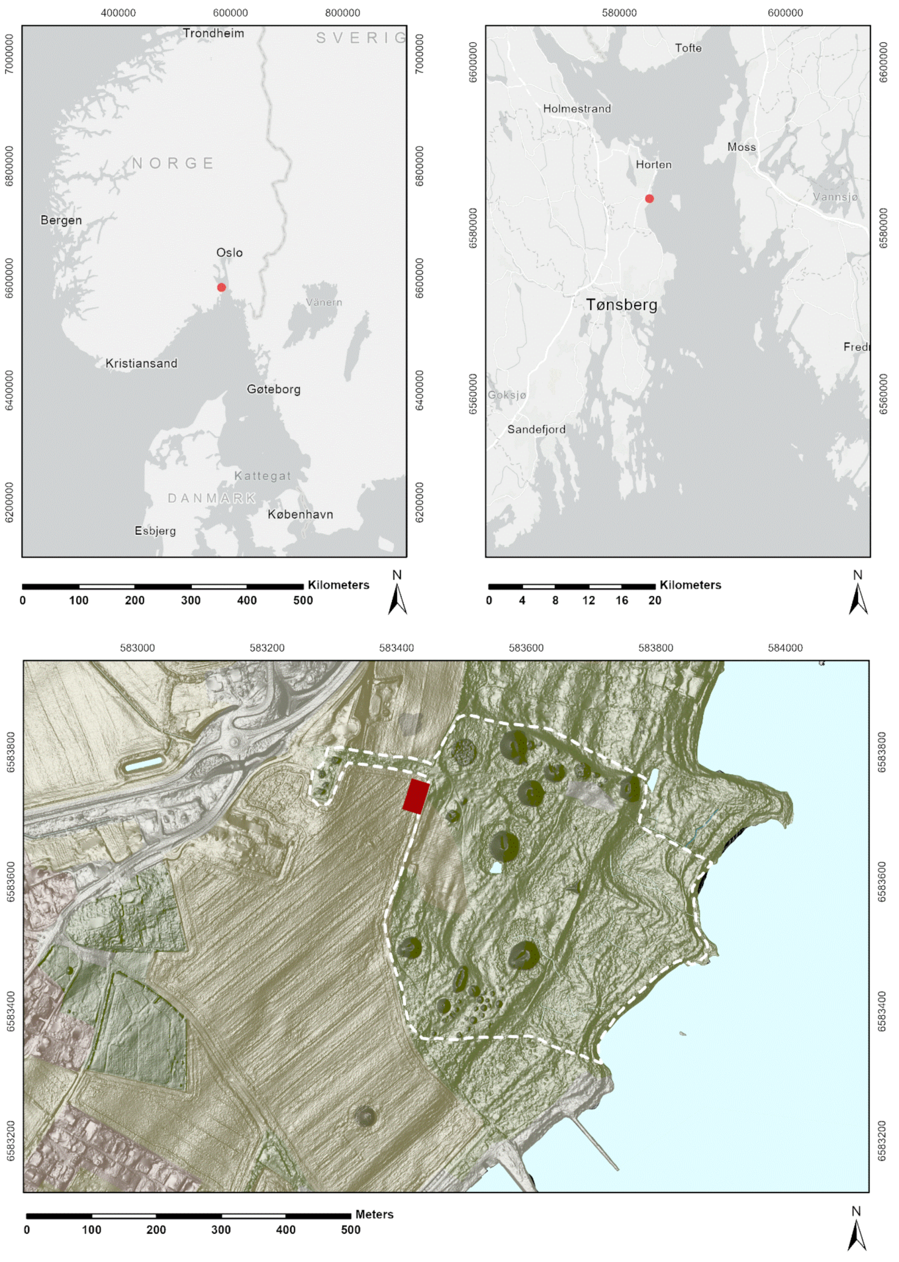
1.2. The Site of Borre

Borre is located in the municipality of Horten in Vestfold and Telemark County, on a gentle slope bordering the western part of the Oslofjord (Figure 2). It is best known for one of the largest groups of Late Iron and Viking Age monumental burial mounds in Scandinavia and has been the subject of a number of excavations and studies [18,19,20,21,22,23]. In 1991, the results of a soil phosphate survey targeting the area over the hall building (Hall A) triggered an excavation, which in turn unearthed several pits and postholes but did not identify them as part of a larger structure [22]. It was not until the GPR surveys in 2007 that these structures were recognised as belonging to a building [1]. Detailed descriptions of the site and the hall buildings can be found in Tonning et al. (2020). The discovery of these buildings has expanded the character of the site and allows for comparisons to be drawn with central places such as Uppsala and Lejre [24] (p. 56), [25] (p. 363).

Geologically, Borre is situated in an area dominated by moderately sorted beach sands over marine clay silt. The beach deposits were formed over the Holocene during post-glacial isostatic rebound, which caused sea levels to gradually retreat. Hall A is located at c. 18–20 m above sea level, which, according to sea-level curves for the region, gives an approximate date of 2400–1900 BCE for its emergence from the sea [26,27]. A little over 100 m west and 7 m higher in elevation runs the top of the Ra moraine, a terminal moraine from the Younger Dryas.

The sediments at the test area retain visible stratified layers from deposition as high energy deposits of gravels and sands. These layered sands and gravels are over 1 m thick at the test site, meaning that they form the parent material of the classified soils present. The underlying marine clay at c. 1.5 m, however, limits drainage in times of high precipitation or snow melt. Within the uppermost metre, there is evidence for the translocation and deposition of iron oxides from repeated saturation and drainage.

Formed from these sands are Haplic Umbrisols (Arenic). Umbrisols are described as soils with a topsoil dark in colour, with over 3% carbon and low base-saturation of cations. The qualifier arenic [28] denotes that the first metre below the base of the topsoil is dominated by sands and gravels. These well-drained, cultivated soils are affected by long- and short-term anthropogenic activity, as indicated by the presence of archaeological subsurface features and the use for modern agriculture. Umbrisols are often managed by liming to adjust the pH, and are artificially fertilised to increase yields, which are taken into consideration when interpreting the analytical data. While the central area with the monumental burial mounds is protected and has been turned into a national park, the area surrounding it is, for the most part, subject to agricultural activities and thus much more exposed to erosion and destruction. Due to the relatively coarse grain size distribution, the soils and sediments are generally well-drained and thus the area does not have drainage ditches otherwise widely seen in this part of Norway.

2. Methods

In the spring of 2016, VTFK was offered to rent an area of c. 0.76 ha covering the two hall buildings for the duration of 14 months, starting at the beginning of June 2016. This unexpected opportunity triggered efforts to set up a pilot study aiming to better understand the reasons for the low quality of the GPR dataset collected in 2015.

The short lead-time of less than six weeks until the start of the project prevented VTFK from applying for external funding. It was, however, agreed upon that such an opportunity had to be seized and that the pilot study was to move forward despite its very limited resources. The budget available was designated to the purchase of in situ monitoring equipment, while all other expenses including man-hours were either volunteered by individuals or provided as in-kind contributions by VTFK and the LBI Arch Pro. The single-channel ground penetrating radar device used in the project was kindly supplied by NIKU.

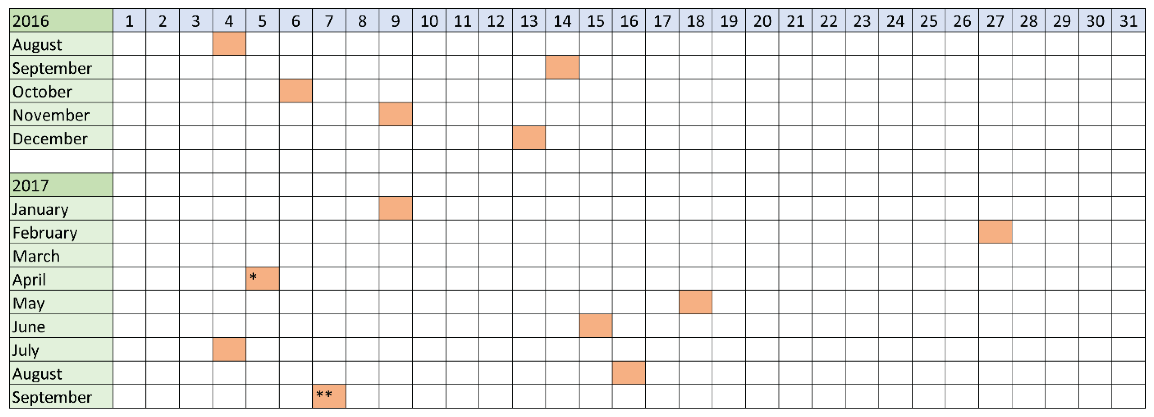
2.1. Monitoring Approach

Ground penetrating radar surveys were conducted roughly once a month across the area covering hall building A for a duration of 14 months to capture potential variations in the data quality throughout the monitoring period (Figure 3). Three monitoring stations were set up to measure the volumetric water content, electrical conductivity, and ground temperature of the subsurface materials in situ to explore the underlying causes for these variations. Monitoring station 1 directly targeted the differences between one of the archaeological features, a posthole belonging to Hall A, and the subsurface materials surrounding it. Monitoring stations 2 and 3 focused on areas undisturbed by archaeological features to the north and south of Hall A to capture the natural background and act as a reference to Monitoring station 1. Their locations were selected based on the GPR data available and a systematic coring survey, which also offered information on the stratification of the site. In addition to the soil sensors, a high-resolution rain gauge was installed at Monitoring station 1 to provide accurate precipitation rates for the test site. A simple meter for snow height measurements was attached to Monitoring station 2. Soil and sediment samples taken from the sections (Figure 4, Figure 5 and Figure 6) dug at the monitoring stations were analysed in the lab to obtain information about the parameters relevant to EM signal propagation.

The test area (30 × 50 m) in which the repeated GPR surveys took place covered most of Hall A, which is located in an arable field bordering the managed grasslands of Borre National Park. The north-eastern corner of the hall is covered by a stone wall that fences the park and is thus inaccessible. Based on the GPR data, the accessible part of Hall A measures 35 × 12 m, and is made up of 59 clearly discernible postholes exhibiting increased signal attenuation with diameters between 0.8 and 1.5 m and depths between 0.25 and 1.3 m [4].

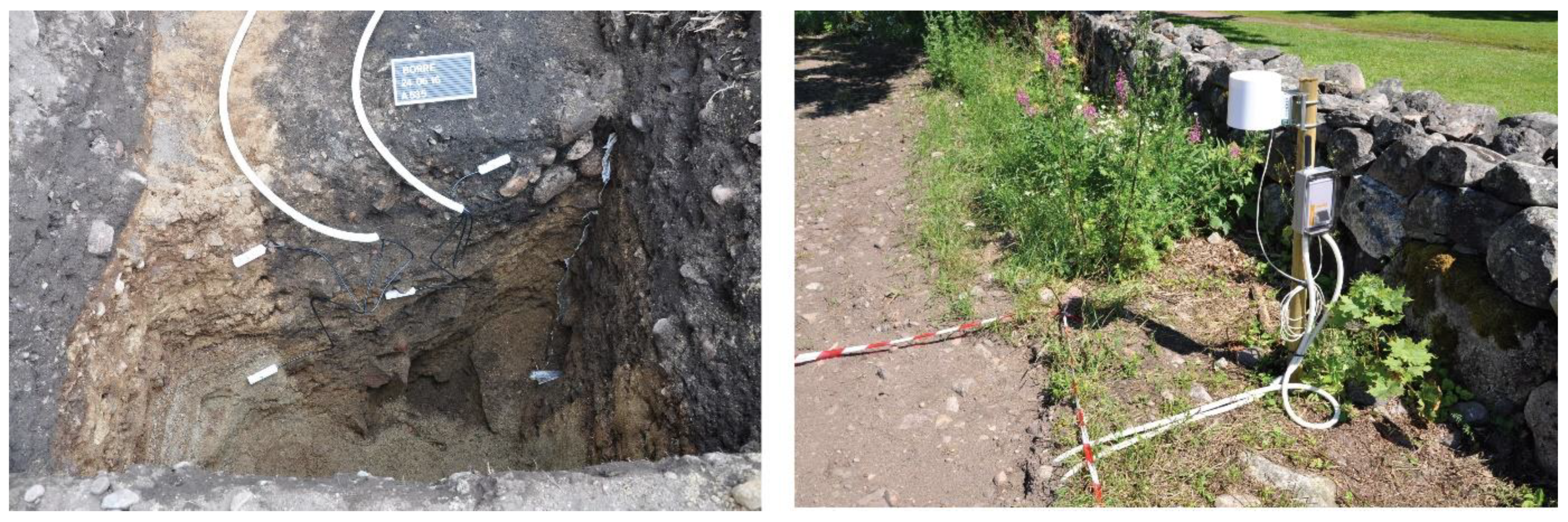
2.2. In Situ Measurements

Three monitoring stations were set up across the survey site to measure the volumetric water content (VWC), bulk electrical conductivity (BEC), and ground temperature of the subsurface materials as well as the precipitation in situ every 10 min (Figure 4).

GS3 soil sensors (Meter, formerly Decagon) calculated the VWC values based on frequency domain reflectometry technology, which measures the apparent dielectric permittivity ε_a of the subsurface materials at a frequency of 70 MHz as a proxy using a 3rd-order polynomial, also known as the Topp equation [29]. Bulk electrical conductivity was obtained through measuring the resistance between two electrodes when applying an alternating electrical current to them. Temperature was measured by a thermistor located close to one of the sensor prongs [30]. Data were recorded by solar-powered EM50G dataloggers and uploaded regularly to a server via the GSM network, which allowed for checking for sensor malfunction and for access to the data in real time. However, a first screening of the data showed that—for reasons unknown—in situ measurements had not been recorded from 21 August 2017, meaning that the last GPR dataset (07092017) in the time-series presented in this study, acquired in September 2017, could not be investigated in as much detail as the other GPR datasets. Precipitation was measured using an ECRN-100 high-resolution rain gauge (Meter, formerly Decagon) using a double-spoon tipping bucket (www.metergroup.com, 27 April 2022).

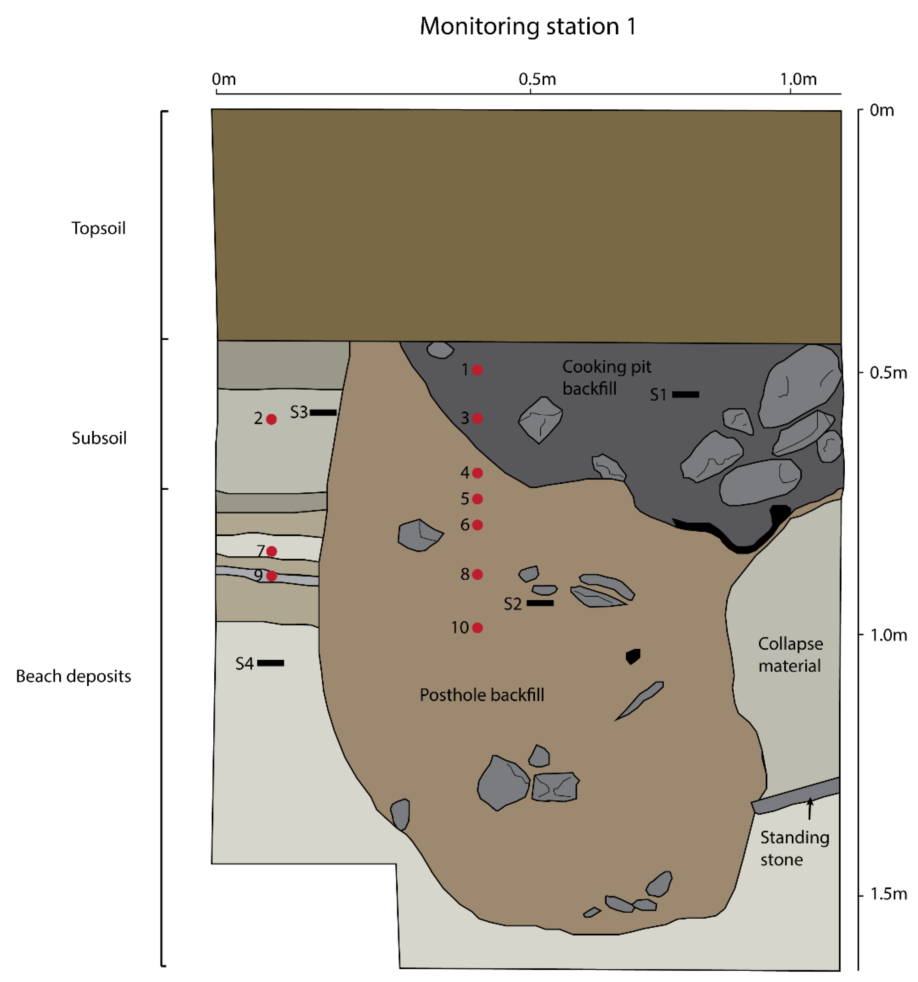
2.2.1. Monitoring Station 1

Monitoring station 1 targeted one of the postholes of Hall A (Figure 5). Due to its protected status, the area of and around Borre is subject to strict provisions based on Norwegian heritage protection laws and archaeological excavations are generally not permitted. It was, however, possible to re-excavate one of the postholes which, during the investigations in 1991, had been only partially dug to record the profile; the other half of the posthole had been preserved.

The exposed section showed an unusually thick sandy topsoil layer (c. 0–40 cm), tentatively attributed to the construction of the hall, which was erected on an artificial terrace (Tonning et al., 2020). Below the topsoil and cut into the actual posthole-backfill was a cooking pit (c. 40–80 cm), a feature frequently found in Norwegian archaeology. Cooking pits are known for their heterogenous backfill, which usually consists of a mixture of organic-rich topsoil material, fire cracked stones, and charcoal [31]. The actual posthole-backfill (c. 40/80–150 cm) turned out to be more homogenous compared to that of the cooking pit, but still showed several layers, indicating a backfill in different phases. Layer 3, for instance, was interpreted as material originating from a collapsed wall. A relatively large, flat stone below the collapse material at the bottom of the backfill (c. 130 cm) was interpreted as a standing stone used to protect the wooden post from drawing moisture through capillary action and thus prolong the building’s lifespan. The posthole itself was cut into stratified beach deposits, representing different depositional events during the postglacial rebound.

To investigate the contrast between the archaeological feature and the surrounding subsurface material, two soil moisture sensors were installed in the cooking pit (c. 60 cm) and the posthole backfill (c. 100 cm), respectively. The two remaining sensors (c. 65 cm and 110 cm) were inserted into the beach deposits to one side of the cooking pit/posthole backfill.

Monitoring station 1 also accommodated the high-resolution rain gauge to measure accurate precipitation rates at the test site.

2.2.2. Background Stations

Monitoring stations 2 and 3 acted as references to Monitoring station 1 and provided information about the natural background of the site by targeting areas undisturbed by archaeological features to the north and south of Hall A (Figure 6). Both monitoring stations showed essentially the same stratification with a topsoil comprised of haplic umbrisol and a layer of subsoil, followed by c. 1 m of stratified beach deposits over marine clay. Soil sensors at station 2 were installed in the topsoil (c. 15 cm), the subsoil (c. 30 cm), and in the beach deposits at c. 50 cm, 70 cm, and 114 cm. The profile at Monitoring station 3, located in a slight depression, includes a thin layer of coarse-grained colluvium between the subsoil and beach sediments. Soil sensors at Monitoring station 3 were installed in the topsoil (c. 14 cm) and in the beach deposits at c. 50 cm, 72 cm, and 115 cm.

2.3. GPR Data Acquisition and Processing

Twelve GPR datasets covering the test area were collected between July 2016 and September 2017 using a single-channel 500 MHz Noggin antenna from Sensors & Software. Surveys were conducted roughly once per month (Figure 7), depending on the available human-power. The survey in April 2017 generated corrupted data and was thus not analysed further. Data positioning was achieved via a grid, set at 25 cm for the cross-line spacing and at fixed distance intervals of 2.5 cm (4-fold trace stacking) for the in-line spacing.

The surface of the test site posed an unexpected problem. As it was not farmed during the monitoring period, vegetation—mainly weeds—started to quickly cover the surface during the growth period in the summer of 2016, and especially in the spring and summer of 2017. In an attempt to keep the test site accessible as well as provide comparable conditions, the farmer harrowed the surface prior to each survey. This initially seemed to help but resulted in a follow-up issue whereby the lack of vegetation increased erosion. Rainfall and surface runoff washed the surface free of the finer material, leaving behind coarser grain size fractions until the test site was covered by large quantities of pebbles and gravel originating from the nearby Ra moraine. While it was still possible to conduct the GPR surveys, the increasingly rougher ground conditions led to a poorer antenna-ground coupling as the monitoring period went on.

Data processing and visualisation were conducted using ApRadar (ZAMG ArcheoProspections^®/LBI ArchPro). To account for the different propagation velocities, a velocity model based on hyperbolae fittings in Reflex W (www.sandmeier-geo.de, 27 April 2022) was generated individually for every dataset. Initially, the buried velocity targets at Monitoring stations 2 and 3 should have provided more accurate velocity estimations, but the targets did not generate discernible reflections in the radargrams, and the idea thus had to be abandoned. To ensure comparability, all datasets were processed using the same set of parameters that included band-pass frequency filtering, time-zero corrections, average trace removal, trace interpolation, 2D Kirchhoff migration, and Hilbert transformation. Data were interpolated into a georeferenced 3D data block and subsequently sliced into depth-slices of the desired thickness. Results were then multiplied by a factor to reach a mean of 100 for each depth slice. The resulting TIFF images were displayed in grey scale and imported into ArcGIS Pro 2.80, which allows for a visual comparison of the different depth-slices acquired at different times using the time- and depth-sliders function simultaneously. Comparisons between the different GPR datasets were also conducted using the in-house developed Python program Schlitzi+, which allowed for the interactive extraction of traces and profiles based on individual depth-slices.

2.4. Soil and Sediment Sampling and Analyses

Samples for the soil and sedimentological analyses were collected from the profiles of Monitoring stations 1, 2, and 3 at every 5 cm (Monitoring station 1 between 50 and 105 cm, Monitoring station 2 between 0 and 115 cm; Monitoring station 3 between 0 and 105 cm). Laboratory-based analyses were conducted at the Institute for Archaeology, Conservation, and History at the University of Oslo and included loss on ignition (LOI) to determine the organic content, particle size distribution, pH, and geochemical measurements. Exact procedures can be found in the Supplementary Materials. As this was a pilot study, the aim was to characterise the physical and chemical properties of the subsurface materials as well as to identify potential factors in the soil’s physical and chemical composition that could influence the geophysical response.

3. Results

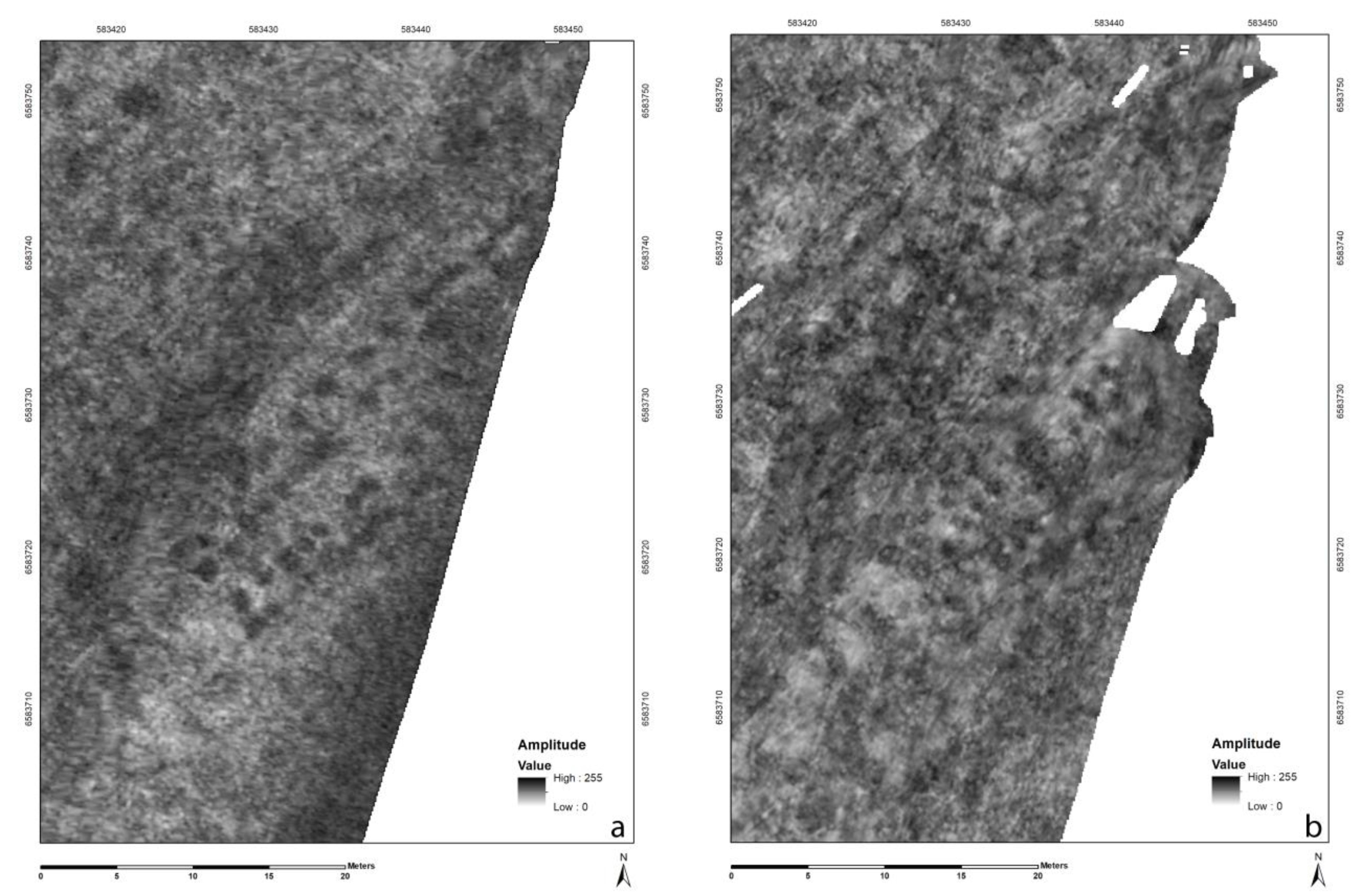
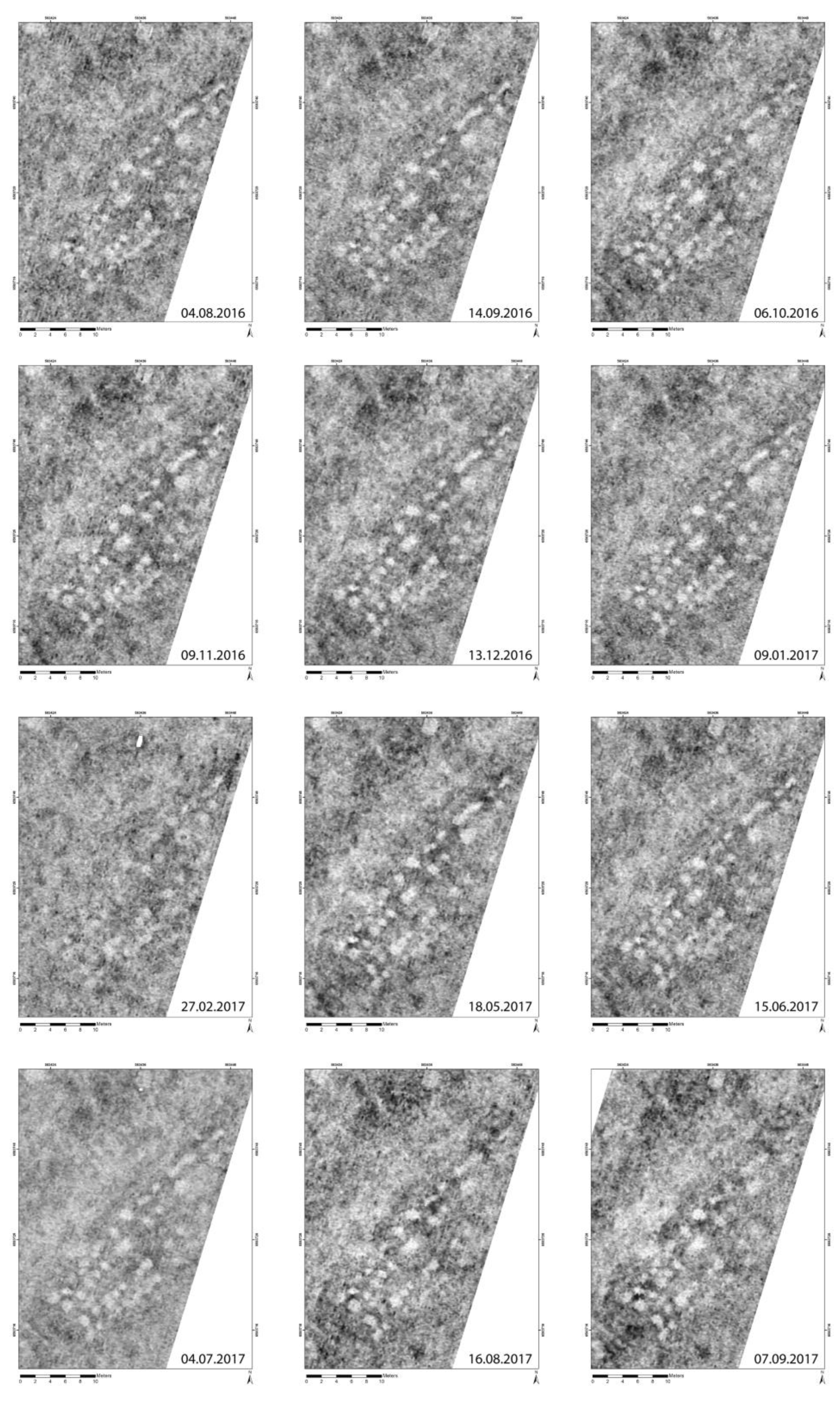
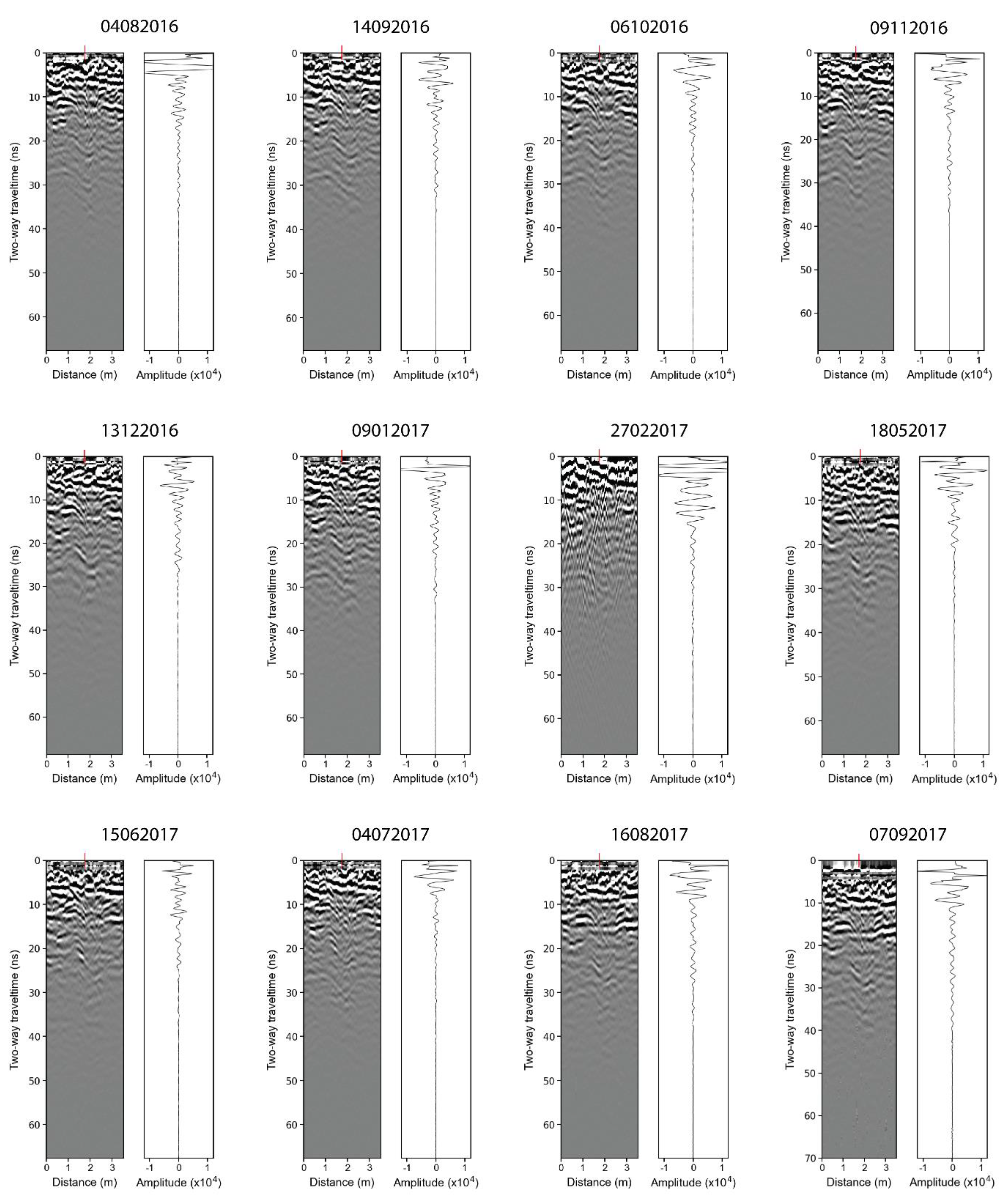
3.1. Comparison of GPR Datasets

In a first step, GPR datasets were classified as of high or low quality. This was conducted qualitatively through visual analysis based on 40–80 cm depth-slices, which carried most of the archaeological information about the hall building as well as quantitatively by means of image and statistical analysis.

3.1.1. Qualitative Analysis of the GPR Data

For the quality grouping, depth-slices (40–80 cm) were inspected visually by three different interpreters in ArcGIS Pro 2.80 using the same display parameters to ensure comparability (Figure 8). (

Table 1. The qualitative classification of datasets into groups of high and low quality.

GPR Datasets	Quality
04082016	low
14092016	high
06102016	high
09112016	high
13122016	high
09012017	high
27022017	low
18052017	low
15062017	high
04072017	high
16082017	low
07092017	low

). This method is obviously subjective, which is why, in an effort to minimise these effects, the two groups were defined by a set of criteria prior to the analysis. Even so, the classifications of all three interpreters differed slightly, mostly regarding the intermediate cases where differences could sometimes be small. Datasets at the upper and lower end of the scale, however, were identified unanimously and these are specifically stated below.

High-quality datasets were characterised through high contrast between the archaeological features and their surrounding subsurface material, clearly discernible postholes and a relatively homogenous, quiet background. Seven of the twelve datasets could be assigned to this group including surveys conducted in September (14092016), October (06102016), November (09112016) and December 2016 (13122016) as well as in January (09012017) and July 2017 (04072017). Among this group, dataset 09012017was considered to show the best depiction of the hall building, followed by 13122016 and 04072017.

Datasets of low data quality were defined by displaying overall low contrast between the archaeological features and surrounding subsurface material and a noisy background, resulting in fewer clearly visible postholes, which complicated mapping of the hall building in its entirety. Datasets in this group included surveys conducted in August 2016 (04082016) as well as in February (27022017), May (18052017), August (16082017), and September 2017 (07092017). By far the lowest quality was shown by the dataset collected in February 2017 (27022017), where the low contrast impeded the recognition of the hall building.

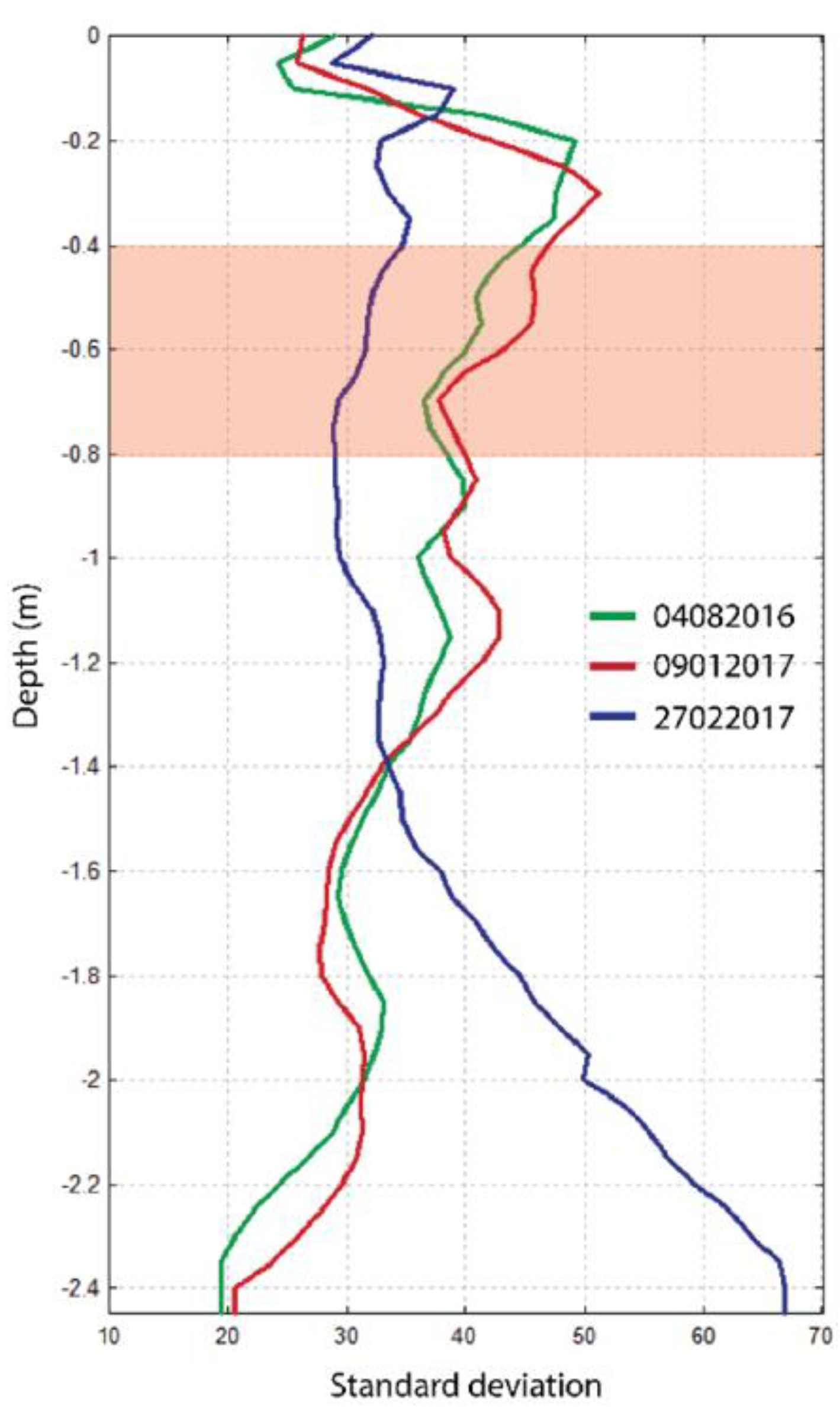
3.1.2. Quantitative Analysis of the GPR Data

A quantification of the differences in data quality was attempted through image and statistical analysis, but proved more complex than initially anticipated.

The analysis of multi-temporal images is one of the main applications in optical space-borne remote sensing. Over the past decades, different supervised and unsupervised change detection algorithms have been developed for this purpose [32]. Of those approaches, the subtraction of (or ratio between) two images are among the easiest ways to visualise differences in raster data. Change detection via image subtraction has been used since the 1970s [33] because it is easy to compute, and the result is straightforward to interpret. For this paper, image subtraction was attempted on the 40 cm–80 cm depth slice of datasets 09012017 and 27022017, respectively, representing the upper and lower limit in the data quality. The raster profiles in the lower-left portion of Figure 9 revealed that high-frequency amplitude changes characterised the original depth-slices. To optimise the legibility of the resulting difference image, both depth-slices were filtered with a 2D Gaussian smoothing kernel with a standard deviation of 2. The resulting subtraction image did highlight some differences in a few of the postholes (see the top right image in Figure 9 and the difference profile). Still, it overall failed to convincingly depict differences in the archaeological information that are easy to perceive by a human observer (Figure 8). Attempts including more advanced algorithms such as iteratively reweighted multivariate alteration detection [34] or local correlation analysis did not noticeably improve the results. The most probable reason for this outcome lies in tiny image mis-registrations (due to minor but dissimilar georeferencing errors) and remaining rapid amplitude changes that are even present in single archaeological features, but dissimilar for both datasets.

A second approach of quantitatively grouping the datasets was undertaken by comparing the standard deviations of the 40–80 cm depth-slices to each other, following the hypothesis that a high standard deviation based on the absolute amplitudes of each depth-slice would indicate higher contrast and thus a higher quality dataset. A standard deviation for the absolute amplitude values of each depth-slice was calculated by first adding the respective values in the time range corresponding to the depths of 0–5, 5–10, 10–15 cm, etc. The results were then multiplied by a factor to reach a median of 100 for each of the amplitude values of each depth slice. A 7 × 7 pixel low-pass filter (70 × 70 cm) was applied to reduce the higher frequency noise. Standard deviations for all measurement points of each depth-slice were subsequently calculated and the median of the respective standard deviations for the desired depth slice range was generated.

This strategy was partially successful and able to confirm datasets 27022017 and 04082016 as the datasets on the lower end of the quality spectrum, showing standard deviations of 31.544 and 40.094, respectively, for the 40–80 cm depth-slice (

Table 2. The standard deviations across all datasets for depth-slices 40–80 cm in descending order, juxtaposed with the qualitative classification.

StdDev 40–80 cm	GPR Datasets	Quality
53.440	07092017	Low
51.501	16082017	Low
49.540	18052017	Low
48.195	09112016	High
47.888	13122016	High
46.811	15062017	High
45.556	06102016	High
42.929	09012017	High
42.885	04072017	High
42.237	14092016	High
40.094	04082016	Low
31.544	27022017	Low

and Figure 10). For the remaining datasets in this depth range, the results showed a rather unexpected grouping: datasets classified as of low quality showed the highest and lowest standard deviations, while datasets of high-quality featured standard deviations in the middle ranges.

Revisiting the depth-slices with this in mind, it seems that the level of background noise (background noise refers here to all unwanted elements in the GPR data including deviations from the desired signal attributable to the device used, to external sources as well as to what is sometimes called “soil noise” [35])—which, if high, can make the data interpretation significantly more difficult—increases the level of contrast, which is reflected by the higher standard deviation values of the respective depth-slice. Depth-slices showing a more homogenous background, in turn, imply a lower contrast and indeed show lower standard deviations, however, the lower noise levels in the background ultimately facilitate an interpretation of the archaeological features.

Taking this into consideration, the results of the statistical analysis only partially support the qualitative analysis of the datasets. However, they do highlight the difference between the term contrast as used in image processing and analysis, which can be described by statistical means such as the standard deviation, and the term contrast as used in archaeological prospection, which can loosely be defined as the difference between areas of archaeological significance and areas without archaeological significance. For the latter, standard deviation as a statistical measure of variation is problematic as it reflects the level of noise rather than the contrast in which a successful archaeological interpretation depends on.

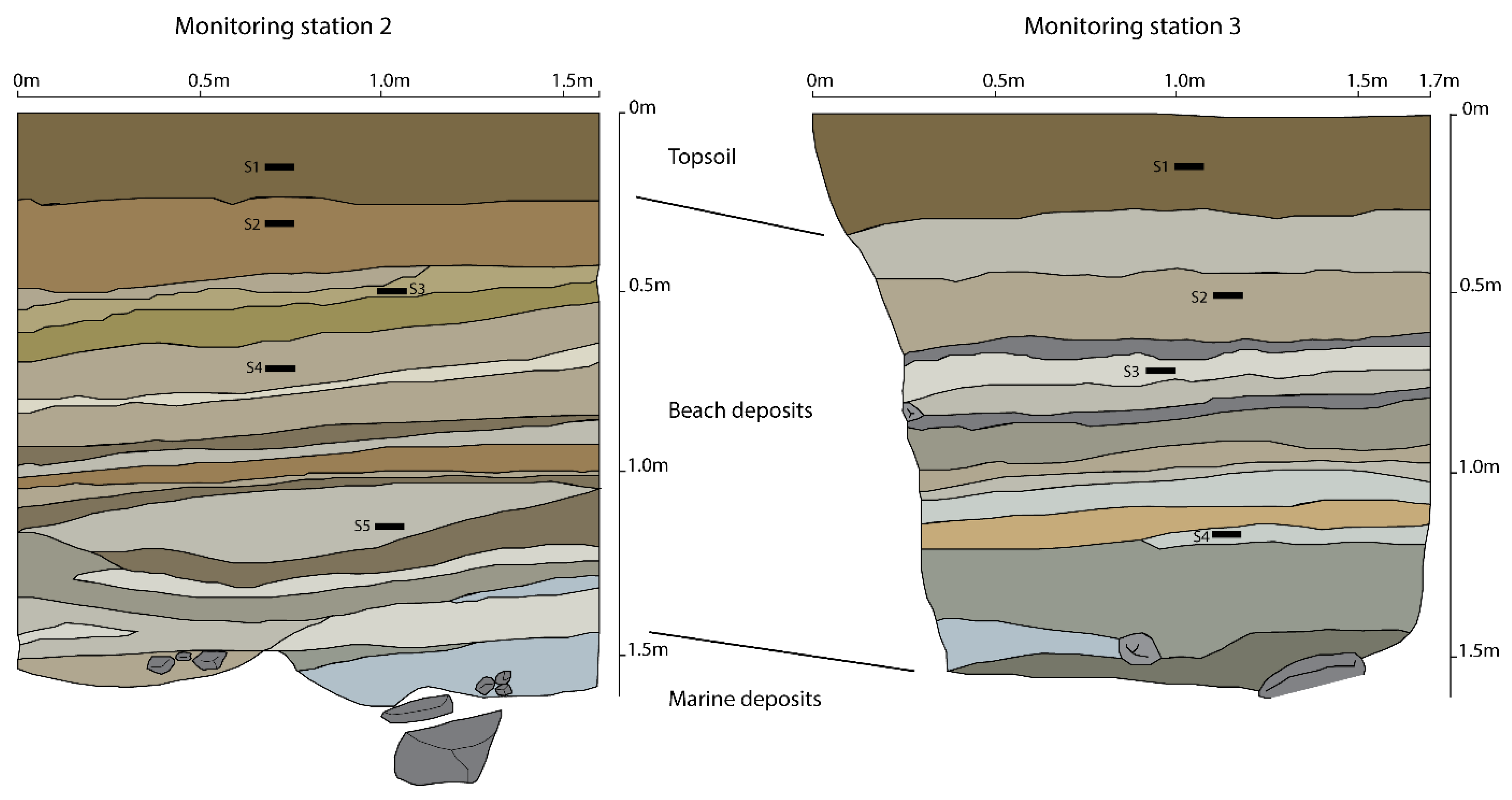
3.2. Soil and Sedimentological Analyses

The soil and sedimentological analyses were focused on a basic characterisation of the subsurface materials present with regard to properties such as particle size distribution and organic matter content, which are pivotal to the soil water infiltration, retention properties, and drainage processes (

Table 3. The basic description of the samples taken from the cooking pit and posthole backfills as well as the subsoil and beach deposits at Monitoring station 1. SA = subangular, SR = subrounded.

Sample Number	Sample Depth		Matrix	Stones and Gravels	Inclusions (Rare X, Common XX, Frequent XXX)	Observations
1	55 cm	Cooking pit backfill	Silt with sand, with organic content (>10%)	c. 2% gravel (=7 small stones), SR and SA (mostly SA). Mixed geology.	Roots and charcoal, very rare (x), larger than 1 mm, in addition to small particles	Highly organic, topsoil, silt and fine sand, with a few stones, homogeneous.
2	65 cm	Subsoil, arenic	Sand with gravel	c. 30% gravel, SA and SR (mostly SA). Mixed geology	Roots, rare (x)	Very fine sand with medium and coarse pebbles
3	65 cm	Cooking pit backfill	Silt with fine sand and gravel, high organic content (>10%)	c. 2% gravel, SA, mixed geology	Charcoal, common (xx), pieces larger than 1 mm	Highly organic, silt and fine sand, humic. Fire-cracked stones
4	75 cm	Posthole backfill	Sandy silt with organic content (>10%).	c. 5% gravel (including two pebbles), SA. Mixed geology	Charcoal, frequent (xxx), larger than 1 mm, in addition to smaller particles	Humic, fine sandy silt, with gravel and very coarse pebbles.
5	80 cm	Posthole backfill	Sand with some silt, with a few gravels. Organic content (<5%)	c. 1% gravel, SR. Mixed geology	Single piece of charcoal, very rare (x), 10 mm long	Very sandy with some silt and gravel.
6	85 cm	Posthole backfill	Very fine sand with silt, with gravel. Organic content (<5%)	c. 2% gravel, SR and SA. Mixed geology	None	Very fine sand with silt, gravel, homogenous
7	90 cm	Beach deposit, fine	Fine sand with two coarse gravels, homogeneous, organic content (<5%)	c. 1% gravel, SR. Mixed geology	None	Gravel shows signs of water rolling/erosion.
8	95 cm	Posthole backfill	Fine sandy silt (approximately 50/50), organic content (c.50%)	c. 2% gravel, SR. Three pebbles. Mixed geology	Charcoal, rare (x) larger than 1 mm, a single piece of burnt hazelnut shell, 5 mm	Very humic sandy silt
9	95 cm	Beach deposit, coarse	Gravel with traces of sand, organic content (<5%)	c.95% gravel, mostly SR and SA. Mixed geology	None	Fine gravel
10	105 cm	Posthole backfill	Fine sand with gravel and pebbles (<50%)	c. 7% gravel, SR and SA. mixed geology	Charcoal, rare (x), larger than 1 mm	Humic, sand

and

Table 4. The results of the LOI analysis for samples taken from the cooking pit and posthole backfills as well as the subsoil and beach deposits at Monitoring station 1.

Sample Number	Sample Depth (cm)	Description	Loss (%)	Organic Carbon (%)
1	55	Cooking pit backfill	4.40	7.59
2	65	Subsoil, arenic	1.27	2.17
3	65	Cooking pit backfill	5.63	9.70
4	75	Posthole backfill	4.78	8.24
5	80	Posthole backfill	1.07	1.85
6	85	Posthole backfill	1.34	2.31
7	90	Beach deposit, fine	1.70	2.93
8	95	Posthole backfill	1.80	2.11
9	95	Beach deposit, coarse	1.74	2.99
10	105	Posthole backfill	6.28	10.83

, see also Section 1.1). Monitoring stations 2 and 3 have no registered archaeological features, and therefore serve as references for the soil and sediment properties on the site, particularly with regard to the topsoil.

Results showed that the physical and chemical differences between the archaeological features and the surrounding subsurface materials were minimal, suggesting that the backfill of the posthole and the cooking pit were largely composed of local sediments.

The particle size distribution of the topsoil samples taken from Monitoring stations 2 and 3 showed a far higher percentage of silt than the lower subsoil. At Monitoring station 1, the cooking pit backfill showed a higher proportion of silt when compared to the subsoil, which exhibited the typical particle size distribution for arenic beach sands, with high fractions of particles over 4 mm (finer and coarser sands and gravels). Silt and clay fractions in the subsoil at Monitoring station 1 were very low, which is consistent with the results from Monitoring stations 2 and 3. The posthole backfill and the surrounding subsurface material showed similar silt and clay fractions, but the overall mineral matrix in the posthole backfill was coarser than the matrix of the surrounding, undisturbed materials and slightly less sorted, particularly when compared to the beach sands at Monitoring stations 2 and 3. This difference, however, was small.

The LOI results of samples 1 (4.4% loss) and 3 (5.63% loss) taken from the cooking pit backfill as well as the upper part of the posthole backfill (sample 4: 4.78% loss) between c. 40 and 75 cm indicated much higher amounts of organic matter than the surrounding beach deposits (sample 2: 1.27% loss). This is unsurprising, as sinkage in the backfill, as the soil settles, and organic decomposition, often results in topsoil filling the top of archaeological features. Below 75 cm, the results were more varied. Differences in the organic content between the samples from the posthole backfill and the surrounding materials significantly decreased to less than 0.5% loss before the values in the posthole backfill suddenly rose to 6.28% loss at around 105 cm. At Monitoring stations 2 and 3, expectedly, the organic content decreased with depth.

The values for pH increased with depth at all monitoring stations. The values in the cooking pit and posthole backfill were overall higher than the upper and surface horizons at monitoring stations 2 and 3 (Figure 3 and Figure 6), but the difference was small and likely caused by the presence of anthropogenic inputs.

The geochemical data (pXRF) suggested elevated phosphorus (P) in the posthole and cooking pit, however, the results were somewhat inconsistent. Unsurprisingly, the higher P and sulphur (S) corresponded to layers with a higher organic content. Trace amounts of copper (Cu) were also associated with the archaeological features, while largely being absent from non-archaeological subsurface materials.

In conclusion, the soil and sedimentological results indicate that the contrast contributing toward the differing geophysical responses seems to originate from a higher amount of silt and organic content in the cooking pit and upper posthole backfill. High percentages of silt and organic matter in the topsoil samples taken from monitoring stations 2 and 3 indicate favourable conditions for water retention, which is of significance for potential EM signal attenuation.

3.3. Environmental Conditions

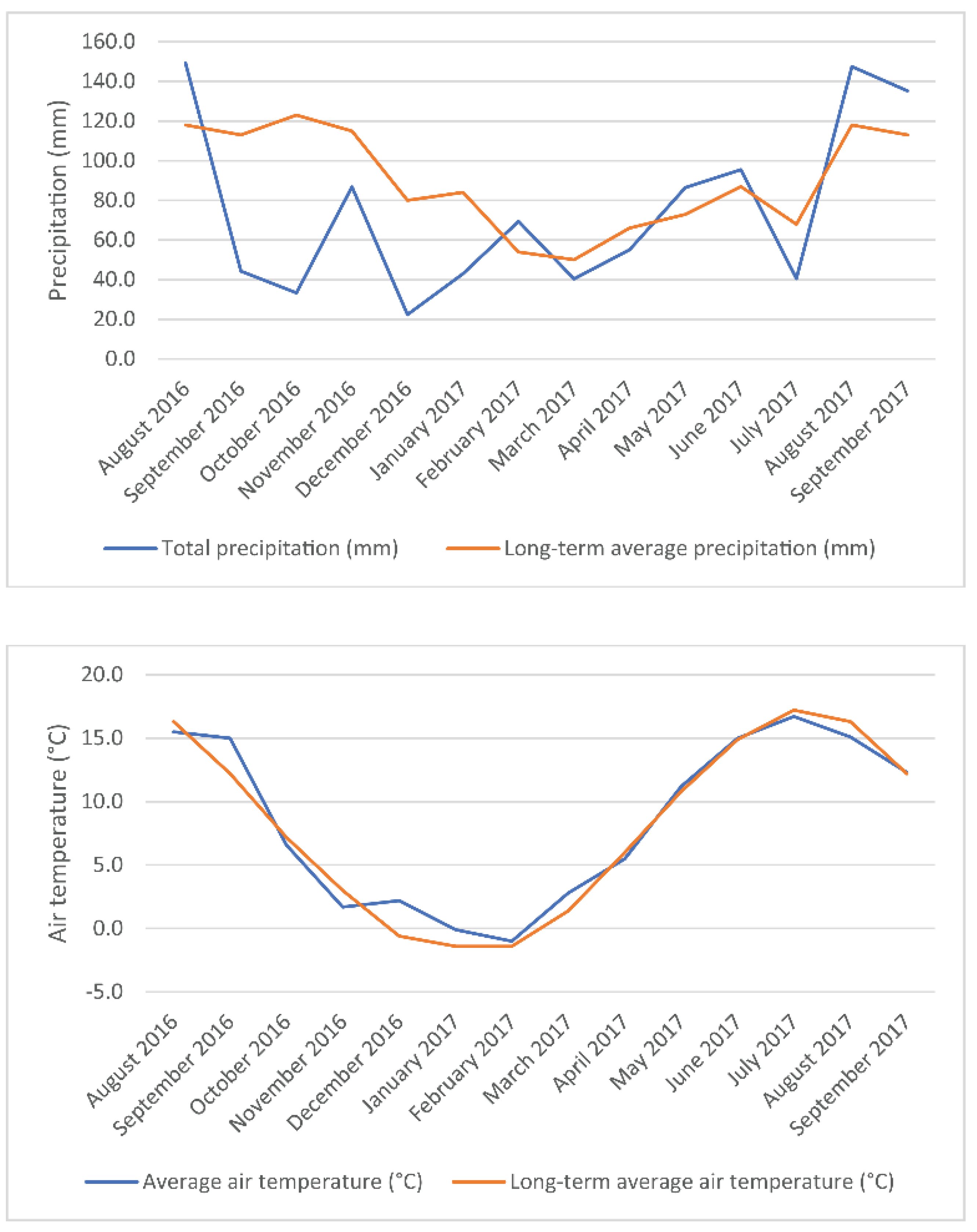
3.3.1. Weather

Observations by the Norwegian Meteorological Institute place the years 2016 and 2017 at around 1 °C above the long-term average air temperature (www.yr.no, 27 April 2022). Local weather data marked the beginning of the monitoring period in August 2016 as slightly colder and wetter than average, followed by very dry conditions throughout the rest of the year (Figure 11). January 2017 was particularly cold and dry before the conditions became wetter in February. May and June 2017 were both warmer and slightly wetter than average, whereas July saw a return to very dry conditions. The two last months of the monitoring period, August and September 2017, were both wetter than average. Snow coverage during the winter of 2016/17 was limited to only a few occasions in February and March 2017 (www.senorge.no, 27 April 2022).

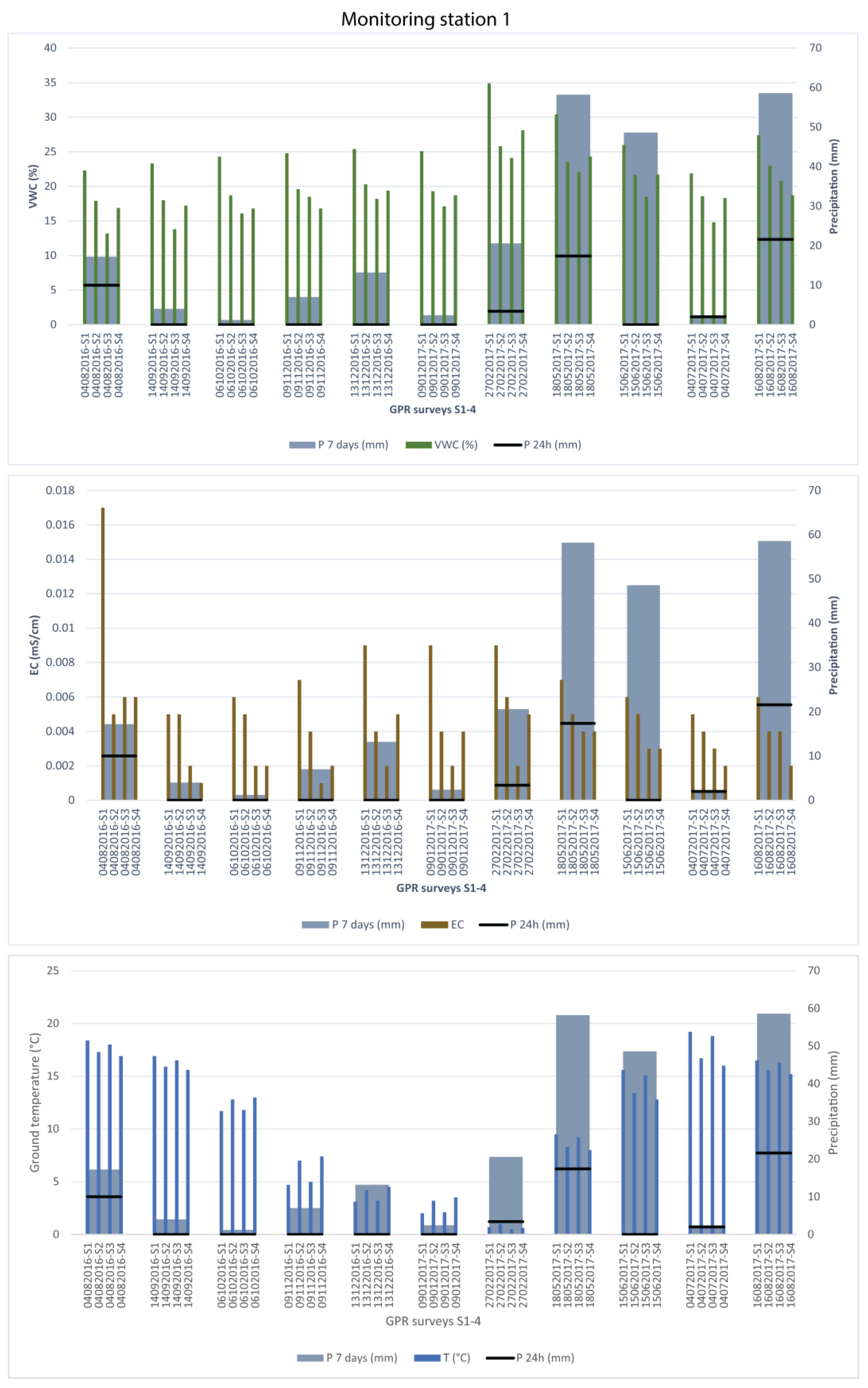
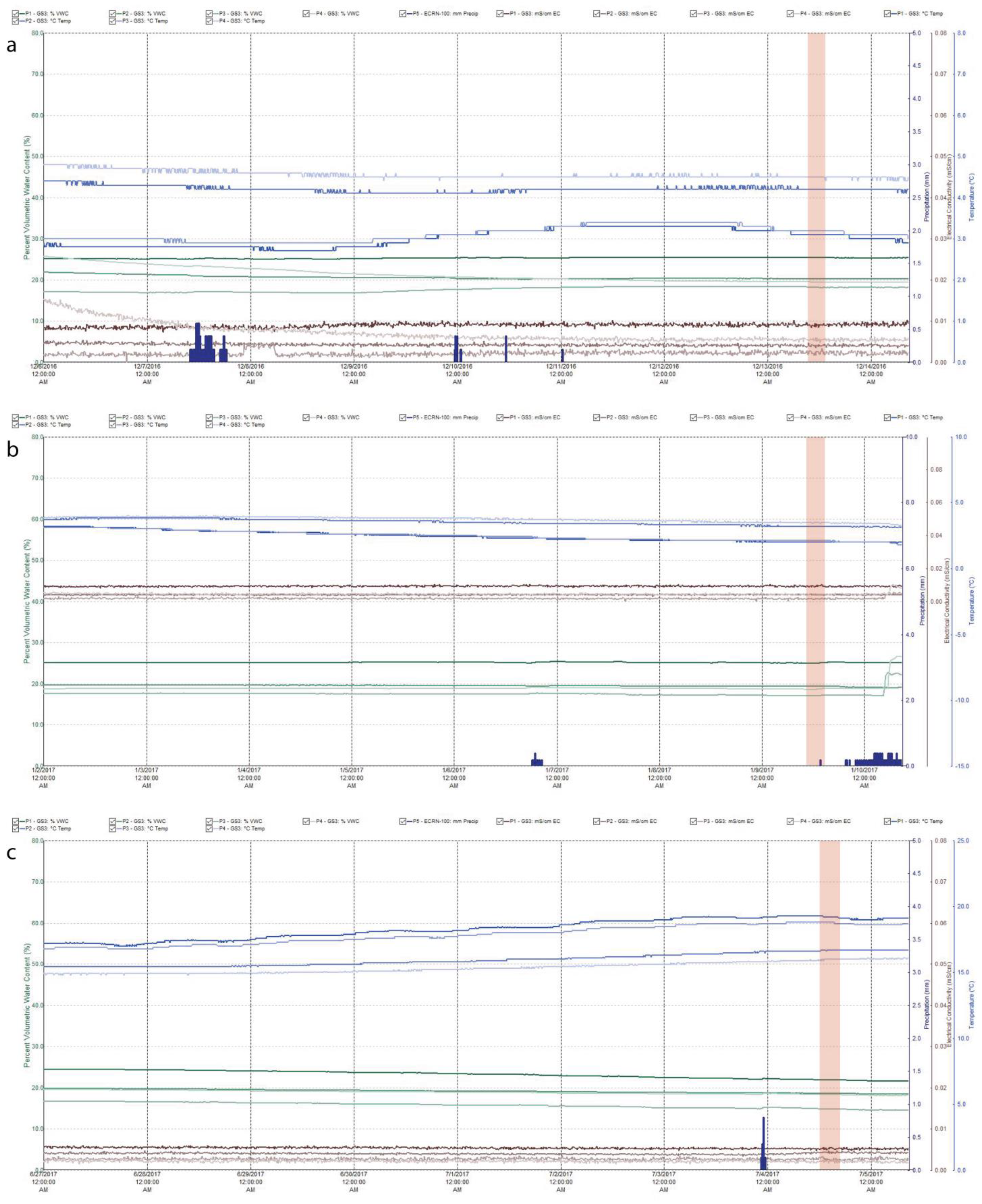
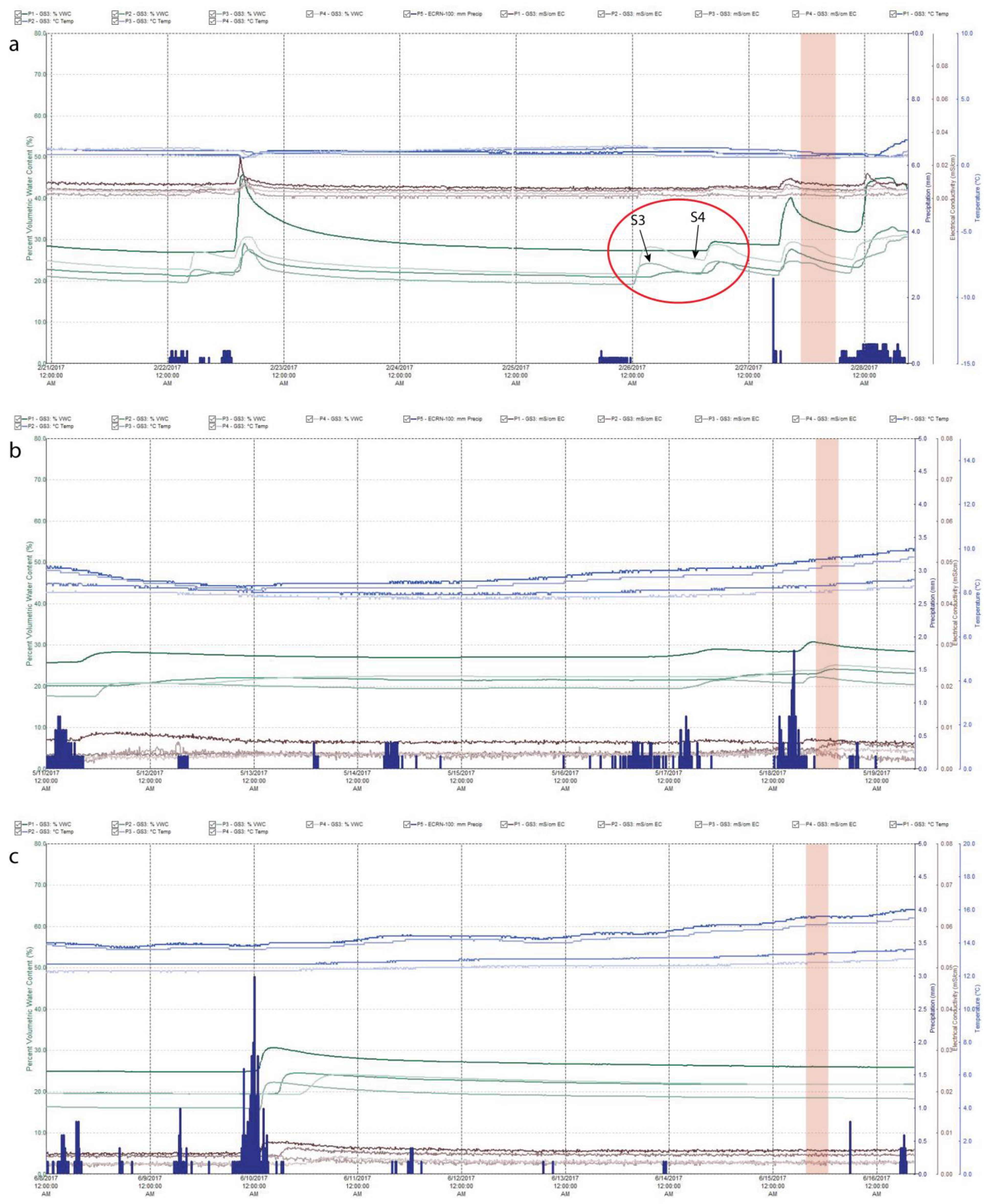
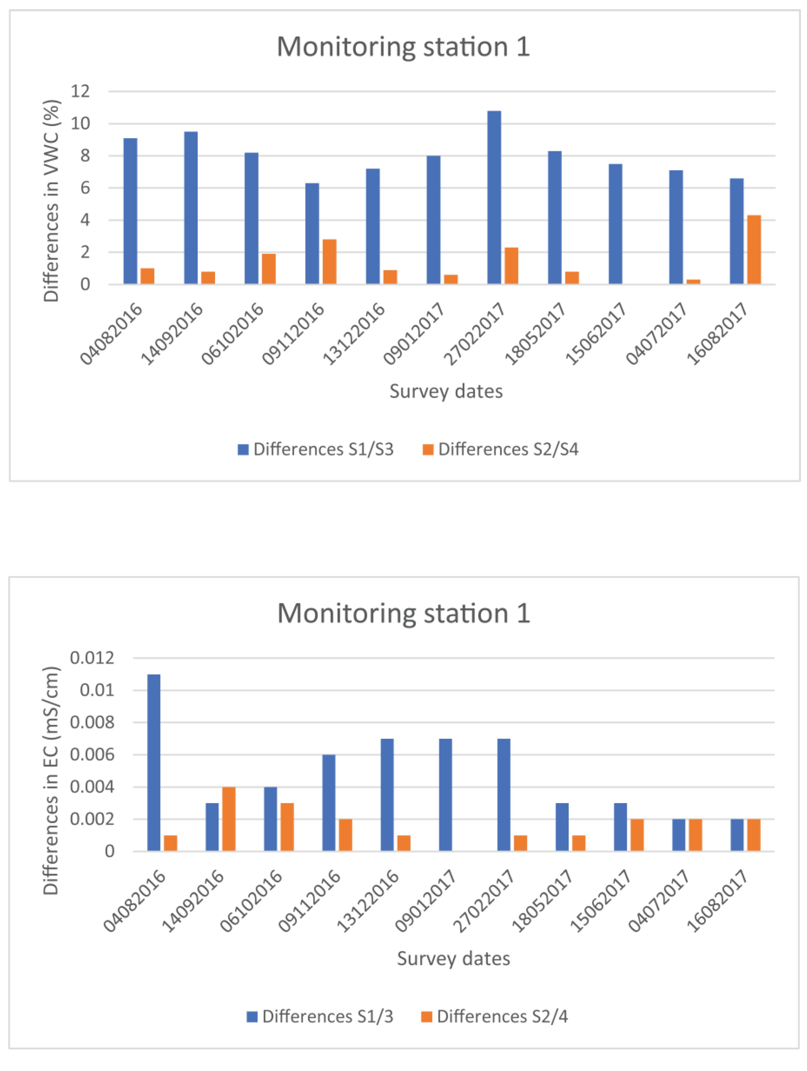
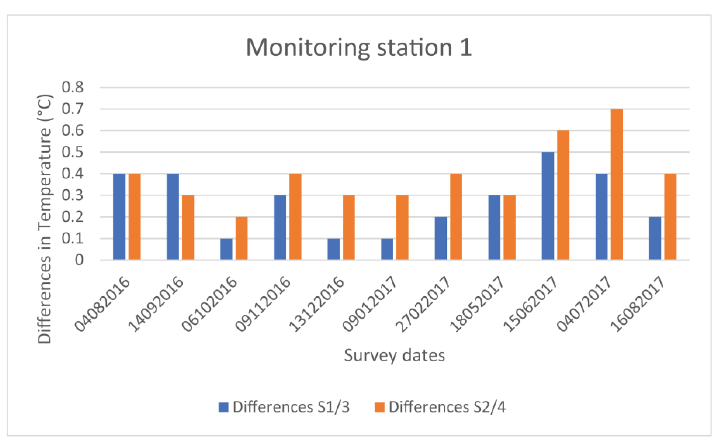
3.3.2. In Situ Monitoring Data

Precipitation data collected by the rain gauge installed at Monitoring station 1 showed a trend similar to the data originating from the public weather station ‘Horten II’, located c. 4 km from Borre, but proved to be more accurate and allowed for a better understanding of the often complex soil moisture variations in the ground (Figure 12).

The VWC measurements indicated drier conditions during the first half of the monitoring period compared to generally wetter conditions later on. The highest overall VWC was measured during the survey in February 2017 (27022017), followed by May 2017 (18052017), August 2017 (16082017), and June 2017 (15062017), while measurements for July 2017 indicated a short return to drier conditions. Looking at the sensors individually, S1, inserted into the more fine-grained and humic cooking pit backfill, showed the highest VWC values across all surveys, while S2, S3, and S4, installed in the posthole backfill and the surrounding beach deposits, respectively, displayed more variation throughout the monitoring period.

Unsurprisingly, the BEC values overall adhered to the same pattern as seen in the VWC measurements with a steady increase in the BEC during the autumn, before plateauing during the winter and decreasing again in the late spring/summer months. The range of the BEC values measured (0.001–0.009 mS/cm) is typical for the sandy material present at Borre.

The ground temperature values follow a seasonal pattern with lower values during autumn and winter and higher values during the summer without ever dropping below freezing. However, while temperatures decreased with depth during the warmer months, the winter months showed a reversal with higher temperatures lower in the soil profile.

To conclude, the in situ monitoring data exhibited a seasonal trend that was expected: a higher VWC and BEC, and lower temperature values in the autumn and winter, indicating colder and wetter conditions, while the summer months displayed lower values in the VWC, BEC, and higher values in ground temperature, reflecting a short period with drier and warmer conditions.

Despite these entirely predictable findings, a closer look at each individual sensor indicated more complex infiltration processes and water movement patterns connected to the prevailing environmental conditions during each of the GPR surveys. While it was beyond the scope of this study to fully disentangle the interplay between all of the different elements, a detailed analysis of the VWC, BEC, and ground temperature recorded before and during the GPR surveys, helps shed light on the factors that influenced the quality of each of the GPR datasets collected.

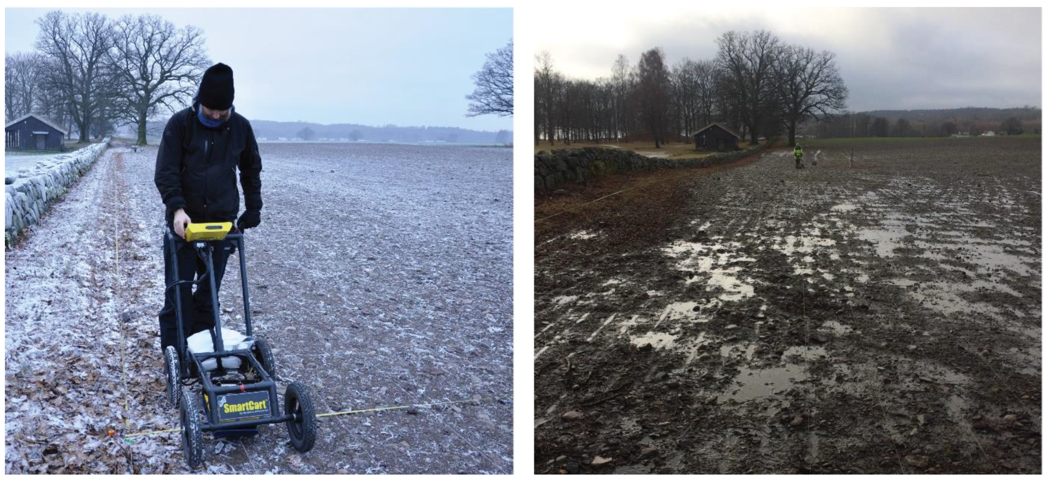
3.3.3. Surveys in Dry Conditions

Six of the twelve surveys were conducted under relatively dry conditions, when less than 5 mm of precipitation had fallen in the week prior to the survey (Figure 13). The 24 h before these surveys did not see any rainfall, except for the GPR data acquired in July 2017 (04072017).

The three surveys undertaken in the autumn of 2016 (14092016, 06102016, and 09112016) showed relatively similar conditions: a few, light rainfall events occurring several days before the respective surveys caused no or only small rises in the VWC that had little to no effect on the GPR data acquired some days after.

The driest conditions prevailed during the survey in July 2017 (04072017) (Figure 13c). The previous 30 days had been warm and dry with little rain, after a wetter period that ended at the beginning of June. Minor rainfall (2 mm) occurred on the evening before the survey, but only minimally affected the VWC recorded by the soil sensors.

The survey in December 2016 (13122016) was conducted after a drier period with the first rainfall (11.8 mm) in three weeks occurring five days before the survey (Figure 13a). Three light rain showers (1.4 mm) occurred three days before the survey. Surprisingly, the VWC and BEC increased only slightly after the bigger rainfall event and did not respond at all to the three lighter ones.

The GPR data in January 2017 (09012017) were acquired under dry, but cold conditions (Figure 13b). Air temperature had dropped below 0 °C on January 2 and reached a minimum of −9.3 °C on January 5. During the remaining four days before the survey, the air temperatures stayed largely below 0 °C. The day of the survey was milder, with temperatures reaching 5.1 °C. The month prior to the survey had been dry, with only 13.2 mm of precipitation, most of which fell on December 24. A light rain shower (2.4 mm) occurred three days before the survey, but did not increase the VWC or BEC values, possibly due to the upper layer of the topsoil being frozen, acting as a barrier and preventing infiltration. This is further supported by photographic documentation taken and observations made during the survey (Figure 14). Without sensors in the upper part of the topsoil, however, the exact course of the frostline remains unknown.

The ground temperatures measured by the soil sensors of Monitoring station 1 ranged between 2 °C and 4 °C but they were buried c. 60 cm below the ground surface and thus most probably not affected by the frozen layer.

3.3.4. Surveys in Wet Conditions

Five of the twelve GPR surveys were conducted during wet conditions (Figure 15). The survey in August 2016 (04082016) was conducted directly after a rainfall event, followed by a rather dry week. A light rain shower on the evening before the survey brought a total of 8.6 mm precipitation. Together with light rainfalls (0.2 mm) at 11:00 the next day and another one (1.2 mm) right before data acquisition, the accumulated precipitation in the 24 h before the survey amounted to 10 mm.

As mentioned earlier, February 2017 (27022017) was mostly characterised by negative temperatures and frost, interrupted by a few warmer periods between February 18 and 23, before the temperatures fell to below 0 °C again. During the night before the survey, the air temperatures steadily rose to reach a maximum of 4 °C around two hours after the survey had started. The varying temperatures in connection to several rainfall events (20.6 mm) in the week prior to the survey spurred the VWC and BEC values across all sensors of Monitoring station 1, suggesting a more complex soil infiltration and percolation pattern compared to those seen in the other datasets (Figure 15a).

The heaviest rainfall, five days before the survey, brought 10.8 mm of precipitation and prompted a marked, yet delayed increase in the VWC, peaking around four hours after the rainfall had ended. Over the course of the next few days, the VWC returned to pre-rainfall levels. A second rainfall (6 mm) c. 36 h before the survey showed a similar water movement pattern with a relatively sudden increase in the VWC several hours after the rainfall had ceased. When looking individually at each soil sensor, however, differences emerged. The VWC measured by S1 and S2, inserted in the backfills of the cooking pit and posthole, remained unaffected until 15 h after the rainfall, when the VWC abruptly rose around 5%, before slowly decreasing again. S3 and S4, installed in the surrounding beach deposits responded quicker to the rainfall, with a steady rise of 5% in the VWC until 5 h after the rainfall, before decreasing again to 3% (see red circle in Figure 15a). Ten hours after the initial rainfall, S3 and S4 exhibited another sudden rise in the VWC of c. 3%. In the time before the third, short, but more intense rainfall (3.4 mm) in the early morning around 3.5 h before the survey started at 9:30, the VWC slightly decreased across all sensors, before the values in S1, S2, and S4 showed a rapid and steep increase c. 2 h after the end of the rainfall, most pronounced in S1 with 11.4%.

While the way water moves through the subsurface is complex and depends on a range of factors, it seems likely that the somewhat erratic changes in the VWC during the February 2017 data acquisition were at least partially caused by a frozen layer in the topsoil. Its response to fluctuations in the air temperature around 0 °C and repeated rainfall events would cause the ground to partially defrost, gradually allowing melt water as well as precipitation to infiltrate the ground. These assumptions are supported by pictures taken from the test site during the survey, which show the ongoing thawing process of the upper topsoil on the day of the survey when air temperatures ranged well above 0 °C. Meltwater seemed to be blocked or at least delayed from infiltrating the ground due to the still partially frozen topsoil, resulting in standing puddles, especially in the north-eastern part of the test area, which formed a wet and muddy surface (Figure 14). These puddles dried up as the survey progressed throughout the day.

The surveys in May, June, and August 2017 were conducted in very wet conditions, characterised by the highest amounts of precipitation recorded for the week prior to the respective surveys. A total of 58.2 mm of precipitation was recorded in the seven days before the survey conducted in May 2017 (18052017), with 33.4 mm of rain in the 48 h right before the survey (Figure 15b). This latter rainfall event increased the VWC between 2% and 3% across all sensors. While S2 and S4 showed continued increase during the survey, values recorded at S1 and S3 decreased almost 1%, indicating the continued drainage.

Ground penetrating radar data in June 2017 (15062017) were acquired after a week that brought 48.6 mm of precipitation, providing some of the wettest conditions during the monitoring period (Figure 15c). In comparison to the May 2017 dataset, however, the bulk of the precipitation (32.4 mm) in June came earlier, five days prior to the survey. This rainfall triggered a marked response and increased the VWC in both S1 (5.7%) and S3 (6.6%). This increase could also be observed in S2 (4.8%), and S4 (4.6%), but with a delay of c. 2.5 h and 7 h, respectively. Three lighter rainfall events in the days before the survey did not prompt any significant change in the soil moisture.

The highest amount of precipitation in the week prior to a survey was measured in August 2017 and totalled 58.6 mm, concentrated in two rainfall events. The first, six days before the survey, brought 31.0 mm and an increase in the VWC of 16% to 31.1% recorded by S1. Marked increases in the VWC and more moderate in the BEC were also shown by S2 and S3, whereas S4 responded more gradually over a longer time. The second rainfall event occurred during the night before the survey and amounted to 21.4 mm of precipitation, prompting only a mild response (2–3% increase) in the VWC across all sensors, possibly because the subsurface materials were approaching saturation after the previous rainfall.

3.3.5. Contrast

Sufficient contrast in the physical and electromagnetic properties between archaeological structures and the surrounding subsurface materials is key to high-quality GPR datasets. To quantify the contrast at Borre, in situ measurements of the VWC, BEC, and ground temperature recorded during each GPR data acquisition were added and averaged to calculate the differences between S1 (cooking pit backfill) and S3 (surrounding upper beach deposits) as well as S2 (posthole backfill) and S4 (surrounding lower beach deposits) (Figure 16). The results showed that the differences in the VWC between S1 and S3 were considerably higher (6.6–10.8%) for all surveys compared to the differences between S2 and S4 (0–4.3%). This was not surprising given the physical and chemical properties of the cooking pit backfill and the materials surrounding it (see also Section 3.2). Differences in the BEC generally followed this trend, except for the September 2016 dataset (14092016), where the contrast in BEC between S2 and S4 was higher than between S1 and S3. Data collected in July and August 2017 (04072017, 14082017) exhibited the same difference in the BEC for both S1/S3 and S2/S4. Ground temperature was only minimally different by <1%. For Monitoring station 1, these results suggest that the absorbing structure visible in the GPR data is primarily caused by the cooking pit, rather than the actual posthole.

Surprisingly, the survey with the highest difference in the VWC and BEC was the dataset acquired in February (27022017), which was established both qualitatively as well as quantitatively as being of the lowest quality. Further comparisons of the differences in the VWC and BEC with the GPR datasets and their respective quality classifications produced inconclusive results.

Based on these observations, one could question the assumption that higher differences in the VWC and BEC are tantamount to higher contrast and would thus automatically produce datasets of higher quality. However, the February 2017 (27022017) dataset was acquired under special environmental conditions in which surface puddles and an ongoing thawing process caused the attenuation and refraction of the EM signal. In addition, the different water retention properties of the subsurface materials have to be taken into account, which, up to a certain point, will enhance the contrast with increasing soil moisture.

All data considered, however, it seems more likely that the number of data points for the respective materials was too low to be representative. The hypothesis behind the attempt to capture the contrast was based on the assumption of three homogenous types of material: the cooking pit backfill, the posthole backfill, and the beach deposits surrounding them. This, of course, is an oversimplification; the excavation showed the cooking pit backfill in particular to be quite heterogenous. The beach deposits were composed of stratified layers of different particle sizes, originating from different depositional events. In addition, due to the heritage protection status of the site, only one archaeological structure could be monitored in situ, creating a pars pro toto approach, which is by nature limited with regard to its representativeness. More sensors at Monitoring station 1 and/or more monitoring stations targeting more archaeological structures across the test area could potentially have provided a more conclusive result. Due to financial limitations, however, this was not feasible in the Borre Monitoring Project.

4. Discussion

4.1. Comparison of High and Low Quality GPR Datasets

Of the seven datasets classified as of high quality (Table 1), six were acquired under dry conditions during the autumn and winter of 2016/17 and the summer of 2017. Compared to an average year, the precipitation rates fell by 60–70% in September, October, and December 2016 and by 50% in January 2017. November 2016 saw more rain, but was still a quarter drier than normal. June 2017 experienced a 40% decrease in rainfall.

These dry conditions were also reflected in the VWC and BEC values measured during each of the GPR surveys: October and November 2016 showed similar conditions, with the VWC between 16 and 24% and the BEC between 0.002 and 0.006 mS/cm and 0.002–0.007 mS/cm, respectively. The VWC and BEC of the December and January datasets were also comparable, ranging between 17 and 25% VWC and 0.002–0.009 mS/cm BEC. The conditions during the September 2016 and July 2017 datasets were even drier, with values ranging from 13.3–23.8% and 13–21% in VWC and 0.001–0.005 mS/cm and 0.002–0.005 mS/cm in BEC.

Even though these months were generally very dry, rainfall events did sporadically occur. However, in all surveys that produced data of high quality, precipitation rates in the week prior to the surveys were low, ranging between 1.2 mm and 13.2 mm, with no or almost no precipitation in the last 24 h. If rainfall events took place such as in the case of the December 2016 dataset (13122016), which saw precipitation (11.8 mm) five days and (1.4 mm) three days before the survey, and the July 2017 dataset (04072017), where light rainfall (2 mm) occurred in the 24 h prior to the survey, it had little to no effect on the VWC and BEC values.

Only the high-quality dataset of June 2017 (15062017) was collected under wet conditions, with 48.6 mm of precipitation in the week prior to the survey. However, the bulk amount fell five days before the survey, allowing time for infiltration and drainage of soil moisture, and no precipitation occurred in the 24 h before the survey. These conditions were also reflected in the in situ measurements with the VWC (18.5–26%) and BEC (0.003–0.006 mS/cm) values ranging slightly higher than during the autumn and winter datasets.

The dataset unanimously classified as the one with the highest quality was collected in January 2017 (09012017) under dry, but very cold conditions, leading to an at least partially frozen topsoil. Water in its frozen state exhibits electric properties that are quite different from when in liquid state, decreasing the attenuation of the GPR signal as it traverses the subsurface [3]. A frozen layer in the ground might also act as a barrier that reduces the soil infiltration capacity depending on factors such as the ice content, soil temperature and soil texture [36] should rainfall occur.

All five datasets classified as of low quality were collected during wet conditions with precipitation in the week prior to the survey ranging from 17 mm to 58 mm, where 10 mm to 21.6 mm fell in the 24 h immediately before the survey. (Precipitation in the 24 h before the September 2017 data collection amounted to 34.9 mm, but data had to be obtained from a weather station 4.2 km from Borre due to a malfunction of the in situ measurements on site).

The precipitation rates in the months of the respective surveys were higher than average by around 110–129% and this is reflected in the higher VWC and BEC values during each of the GPR surveys in August 2016 (27.4–18.7% VWC, 0.002–0.006 BEC), February 2017 (24.1–34.9% VWC, 0.002–0.009 BEC), May 2017 (22.1–30.4%VWC, 0.004–0.007 BEC), and August 2017 (27–18% VWC, 0.002–0.006 mS/cm BEC).

All data considered, it seems that the combination of generally wetter conditions originating from higher amounts of precipitation in the weeks, and especially in the seven days prior to the survey together with a rainfall event in the 24 h before the survey, had an adverse effect on the quality of the GPR data. This observation is supported by the survey in June 2017 (15062017), when a considerable amount of rain fell in the week prior to the survey, but with five days until the survey and no additional precipitation in the 24 h before the survey, the water had sufficient time to drain, resulting in GPR data of higher quality.

The dataset acquired in February 2017 (27022017)—considered unequivocally as of lowest quality—stands out, as it shows the highest VWC and BEC values measured across all of the datasets, but the precipitation rates in the week (20.6 mm) and the 24 h before (3.4 mm) the survey were considerably lower compared to the datasets acquired, for example, in May and August 2017. This observation can be explained by a partially frozen ground following a longer period of low temperatures in the first three weeks of February. In contrast to the January 2017 dataset (09012017), however, where these conditions proved favourable, the sudden rise in temperatures right before the survey caused a part of the frozen ground to thaw, which not only resulted in a steep increase in the VWC over the course of only a few hours, but also reduced the soil infiltration capacity. As a result, surface puddles formed, which are known to impede the EM signal from entering the subsurface. The remaining signal penetrated the topsoil amid an ongoing thawing process, where soil water was changing from frozen to liquid state, exhibiting very different electrical properties between the two. The resulting strong reflections of the EM signal seen in a radargram and trace taken from a profile through one of the undisturbed postholes of Hall A evidence these rapidly changing EM properties throughout the topsoil [37] (Figure 17). Differences in EM properties are also known to change the propagation velocity as the signal travels further downwards. This can lead to refraction and to a reduction in the frequency of the EM signal, which in turn increases the wavelength, thereby diminishing the vertical resolution [5].

4.2. Influence of Environmental Factors

Eleven out of twelve GPR surveys conducted during the monitoring period did in fact detect the hall building. Only the dataset acquired in February 2017 failed to do so. Such a result is encouraging for the use of GPR as a method in research and as a primary investigation tool in CHM, not least because geophysical prospection is not yet fully accepted by the Norwegian archaeological community. However, it is important to bear in mind that the test site consists of sandy, well-draining subsurface materials and the results might thus convey an overly optimistic picture of how much precipitation a site generally can tolerate with regard to a successful GPR survey. Furthermore, the environmental conditions present were not factored in when selecting dates for the GPR surveys, but instead depended on the available resources as well as on common fieldwork practice that aims to avoid extreme weather (e.g., a saturated ground or high rainfall events). As such, the data collected during the monitoring period might include a certain bias toward favourable conditions, but this approach very much relates to the realities in GPR data acquisition.

The GPR data collected over the course of 13 months clearly indicated differences in the quality. Based on the data analyses presented in this study, these differences did indeed correspond to several different environmental conditions encountered during the monitoring period. First and foremost, the variation in soil moisture, particularly within the finer-grained, organic-rich topsoil. Heavy rain, especially when falling in a short amount of time, can bring the topsoil close to saturation as the amount of water exceeds the drainage capabilities of the subsurface materials. The more water in the ground, the higher the EM signal attenuation. If the contrast between the archaeological feature and the subsurface material is rather small to begin with, as is the case in Borre, attenuation of the signal can interfere with feature detection. With respect to contrast, the situation is more complex: a certain amount of water can in fact increase the contrast in the physical properties between different materials due to their different water retention properties, as became evident in the February 2017 dataset (see Section 3.3.5). However, increased contrast becomes pointless if the EM signal is unable to penetrate the ground.

It was notable that the distribution of the high and low quality datasets did not follow a seasonal pattern, evidenced among others by the datasets considered of highest (09012017) and lowest (27022017) quality, which were acquired in the consecutive months of January and February 2017. Instead, the quality seemed to respond to local weather patterns that govern the soil moisture content present in the ground during the surveys, in particular rainfall events as well as the freezing and thawing processes of the upper soil in the days before the surveys. Similar observations have been made by other researchers [5,8].

The results of the analysis support the long-standing rule that dry conditions are beneficial for the quality of a GPR survey, whereas wet conditions can lead to increased signal attenuation, which, together with low contrast, is ultimately detrimental to the detection of archaeological structures. However, how much soil moisture is too much before a GPR survey becomes meaningless?

A closer look indicates that several weeks of no or very low precipitation was necessary to obtain datasets of the highest quality. The longer this period, the drier the subsurface became and the less prone it was to reach a critical soil moisture content when rainfall did occur.

Dry conditions and air temperatures below 0 °C, which caused the topsoil to partially freeze, produced the best result, as evidenced by both the December 2016 (13122016) and January 2017 (09012017) datasets. The potential for collecting data of high quality during the winter was unexpected, mainly because the winter months are generally not regarded as a suitable field season for geophysical prospection in Norway and thus not many examples of GPR datasets acquired during this period exist. Frozen soil water, particularly in the often organic-rich topsoil, reduces the attenuation of the GPR signal, allowing more energy to penetrate the ground, and facilitates the imaging of the subsurface [3]. Unfortunately, the monitoring period in 2016/2017 did not yield a sustainable snow cover that was suitable for the GPR device to drive on and thus no data could be collected under these conditions. A different study by [3], however, reported on an attempt to survey under different snow conditions using a motorised MALÅ MIRA GPR device including a survey driven over the test site at Borre in 2018, albeit at a time when the soil sensors had already been removed. The promising results obtained during the Borre Monitoring Project could lead to more attention on the winter as a suitable field season. Aside from the advantages in terms of the quality of the datasets, winter surveys could widen the relatively narrow periods in the spring and autumn during which farmers allow motorised GPR surveys to be conducted on cultivated fields after harvest and before sowing.

Datasets of low quality acquired during the monitoring period were caused by large amounts of precipitation shortly before the surveys without sufficient time for the water to drain, particularly when rainfall occurred in the 24 h window before the survey. The situation was exacerbated when the subsurface must already have been close to saturation from previous rainfall. The combination of a partially frozen ground together with a sudden rise in air temperatures, leading to surface puddles and/or the presence of water in both its liquid and frozen state in the topsoil, is a scenario where a GPR survey can fail, even though no rainfall has occurred. Thus, close attention needs to be paid should such a weather pattern be imminent. Methodologically, the GPR data collected in January and February 2017 highlighted the importance of monitoring the frostline, which today, ironically, is measured often times indirectly by using GPR, but was not attempted here. For future monitoring projects, frost tubes would present a simple and cost-efficient way to obtain frostline data.

This latter situation emphasises that the amount of precipitation does not equal the soil moisture content. Infiltration rates are affected by surface runoff, particularly evapotranspiration, and, as mentioned earlier, water movement through the subsurface, which itself is controlled by a range of factors. To fully disentangle the connection between the precipitation rates and soil moisture content is, in short, complex, and was beyond the scope of this study. Basic insights into the infiltration and water movement patterns at the test site before and during the GPR surveys through a high-resolution sampling rate of in situ soil moisture measurements, however, still aided in our understanding of the environmental factors that led to the variation in the GPR data quality.

Due to the range of factors involved in determining the moisture content in the subsurface, it is unsurprising that the findings of this study are valid only for a combination of environmental settings and types of archaeology similar to the ones found at Borre, even though the beneficiary effect of dry conditions with regard to the attenuation of the GPR signal is universally valid. This applies in particular to the amount of precipitation tolerated, as Borre is located on well-draining, sandy soils and sediments, which is consistent with the very low BEC values measured by the monitoring stations. Sites situated on finer, more clayey grounds might tolerate far less soil moisture before a GPR survey becomes meaningless. This hypothesis is supported by the preliminary findings of one of the test sites established in the follow-up project The Vestfold Monitoring Project (VEMOP) (https://www.vtfk.no/meny/tjenester/kultur/kulturarv/vemop/, 27 April 2022). Hovland is situated on finer-grained Umbrisol and exhibits much higher BEC values ranging between 0.018 and 0.39 mS/cm. Here, the archaeological features are often not visible at all in GPR datasets acquired under wet conditions.

In this context, the question arises as to whether in fact any of the GPR data acquired at Borre, with the exception of the February 2017 dataset, are of “low” quality? Within this study, there were clear differences in quality that could be attributed to varying soil moisture within the ground and at the surface. How the GPR datasets from Borre should be ranked quality-wise in a broader context, remains to be seen.

One could ask whether the complexity of the issue and the fact that the results of this study are not readily applicable to other sites would warrant the effort. The answer to this must be yes and no. If we wish to improve the effectiveness of GPR as an archaeological prospection method, increasing our understanding of the influence that the environmental settings and processes exert over the quality of GPR data is paramount. However, a study such as the Borre Monitoring Project obviously cannot be conducted for every survey site. A solution could be to focus instead on different combinations of environmental settings and types of archaeological features representative for a geographical region, an approach currently pursued byVEMOP.

From a practical perspective, the acquisition of GPR data under ideal conditions will not always be possible. Commercial providers seldom have the time and/or capacity to wait until the ground has dried sufficiently, while CHM authorities and developers must adhere to legal obligations and contractually agreed schedules. However, knowledge about the potential effects of collecting GPR data under less-than ideal conditions as well as the consequences of basing decisions on the interpretation of lower quality datasets can aid in setting corrective actions such as a follow-up using extended topsoil stripping or excavations.

5. Conclusions

The results of this study clearly demonstrate that environmental factors, particularlyprecipitation rates and variations in soil moisture content in the subsurface materials, affect the quality of GPR data. Of the 12 GPR datasets collected during the monitoring period, seven proved to be of high quality, where the archaeological features were clearly visible with good contrast to the surrounding subsurface materials and a relatively homogenous, quiet background. The majority of the GPR datasets in the high-quality group were collected during dry conditions, when minimal rainfall had occurred in the three weeks before the survey.

Five datasets were classified to be of low quality. This group displayed lower contrast between the archaeological features and the surrounding subsurface materials and increased noise in the background, which together complicated the interpretation of these datasets. Only one dataset failed to depict the hall building. All of the datasets in the low quality group were collected under wet conditions, with high precipitation rates in the week, and especially in the 24 h prior to the survey.

Ground penetrating radar datasets of the highest and lowest quality were collected in consecutive months during the winter, indicating that the quality did not correspond to seasonality, but to smaller-scale, regional weather patterns. Ground penetrating radar surveys conducted during the winter months generated datasets of the highest quality, but required dry and very cold conditions and a partially frozen topsoil. However, asdata analysis has shown, such favourable conditions can quickly change due to rising temperatures, and lead to unsuccessful survey outcomes. Winter in this part of the world should nonetheless be more frequently considered as a season for fieldwork.

The results of the study have demonstrated how important it is to consider the environmental factors throughout all stages of a GPR survey. Should a survey under favourable conditions not be possible due to external circumstances, then practitioners and stakeholders must at least be familiar with the consequences, so that appropriate measures can be undertaken to counteract potential issues.

The Borre Monitoring project was conducted as a pilot study with limited resources. The monitoring approach proved successful, but the results highlighted the importance of paying more attention to the frostline and the topsoil in future projects.

Due to the nature of this research, the results presented here are valid only for sites that show similar settings to Borre. Further research should be focused on expanding the knowledge of how EM signal propagation responds to other soils and sediments frequently found at Norwegian sites under varying environmental conditions. Such research could optimise the planning of GPR surveys, thus increasing the likelihood of acquiring high-quality data as well as helping to convince the Norwegian archaeological community and authorities/stakeholders of the potential of GPR.

References

1. Trinks, I. (University of Vienna, Vienna, Austria). Borre October 2007. Unpublished Report Prepared for Vestfold County Council. 2007. [Google Scholar]
2. Sala, J. (3D Radar, Oslo, Norway). Informasjon om Borreparken. Unpublished Report Prepared for Vestfold County Council. 2008. [Google Scholar]
3. Gabler, M.; Trinks, I.; Nau, E.; Hinterleitner, A.; Paasche, K.; Gustavsen, L.; Kristiansen, M.; Tonning, C.; Schneidhofer, P.; Kucera, M.; et al. Archaeological Prospection with Motorised Multichannel Ground-Penetrating Radar Arrays on Snow-Covered Areas in Norway. Remote Sens. 2019, 11, 2485. [Google Scholar] [CrossRef] [Green Version]
4. Tonning, C.; Schneidhofer, P.; Nau, E.; Gansum, T.; Lia, V.; Gustavsen, L.; Filzwieser, R.; Wallner, M.; Kristiansen, M.; Neubauer, W.; et al. Halls at Borre: The discovery of three large buildings at a Late Iron and Viking Age royal burial site in Norway. Antiquity 2020, 94, 145–163. [Google Scholar] [CrossRef]
5. Boddice, D. Changing Geophysical Contrast between Archaeological Features and Surrounding Soil. Ph.D. Thesis, University of Birmingham, Birmingham, UK, 2014. [Google Scholar]
6. Schultz, J.J. Sequential Monitoring of Burials Containing Small Pig Cadavers Using Ground Penetrating Radar. J. Forensic Sci. 2008, 53, 279–287. [Google Scholar] [CrossRef]
7. Linck, R.; Fassbinder, J.W.E. Determination of the influence of soil parameters and sample density on ground-penetrating radar: A case study of a Roman picket in Lower Bavaria. Archaeol. Anthr. Sci. 2013, 6, 93–106. [Google Scholar] [CrossRef]
8. Fry, R. Time-Lapse Geophysical Investigations over Known Archaeological Features Using Electrical Resistivity Imaging and Earth Resistance. Ph.D. Thesis, University of Bradford, Bradford, UK, 2014. [Google Scholar]
9. Annan, A.P. Electromagnetic principles of ground penetrating radar. In Ground Penetrating Radar Theory and Applications; Jol, H.M., Ed.; Elsevier Science: Amsterdam, The Netherlands, 2008; pp. 1–40. [Google Scholar] [CrossRef]
10. Conyers, L.B. Ground-Penetrating Radar for Archaeology, 3rd ed.; Altamira Press: Lanham, MD, USA, 2013. [Google Scholar]
11. Cassidy, N.J. Electrical and magnetic properties of rocks, soils and fluids. In Ground Penetrating Radar Theory and Applications; Jol, H.M., Ed.; Elsevier Science: Amsterdam, The Netherlands, 2008; pp. 41–72. [Google Scholar] [CrossRef]
12. Scollar, I.; Tabbagh, A.; Hesse, A.; Herzog, I. Archaeological Prospecting and Remote Sensing; Topics in Remote Sensing 2; Cambridge University Press: Cambridge, UK, 1990; p. 696. [Google Scholar]
13. Visconti, F.; de Paz, J.M.; Martínez, D.; Molina, M.J. Laboratory and field assessment of the capacitance sensors Decagon 10HS and 5TE for estimating the water content of irrigated soils. Agric. Water Manag. 2014, 132, 111–119. [Google Scholar] [CrossRef]
14. Doolittle, J.A.; Butnor, J.R. Soils, peatlands, and biomonitoring. In Ground Penetrating Radar Theory and Applications; Jol, H.M., Ed.; Elsevier Science: Amsterdam, The Netherlands, 2008; pp. 197–202. [Google Scholar]
15. Donahue, R.L.; Miller, R.W.; Shickluna, J.C. Soils: An Introduction to Soils and Plant Growth, 4th ed.; Prentice-Hall: Hoboken, NJ, USA, 1977; p. 626. [Google Scholar]
16. Tan, K.H. Principles of Soil Chemistry; Marcel Dekker, Inc.: New York, NY, USA, 1998; p. 320. [Google Scholar]
17. Cates, A. The Connection between Soil Organic Matter and Soil Water; Minnesota Crop News; Minnesota University Extension. 2020. Available online: https://blog-crop-news.extension.umn.edu/2020/03/the-connection-between-soil-organic.html (accessed on 11 June 2022).
18. Nicolaysen, N. Om Borrefundet i 1852, Foreningen til Norske Fortidsminnesmerkers Bevaring; Foreningen til Norske Fortidsmin-Nesmerkers Bevaring: Kristiania, Norway, 1854; pp. 25–30. [Google Scholar]
19. Brøgger, A.W. Borrefundet og Vestfoldkongenes graver; Videnskapsselskapet Skrifter II. Hist. Folisofisk Kl. 1916, 1, 1–67. [Google Scholar]
20. Blindheim, C. Borre i lys av Borre-funnet og Nasjonalparken. In Borre Bygdebok; Lillevold, E., Ed.; Borre Kommune: Horten, Norway, 1954; pp. 1–26. [Google Scholar]
21. Myhre, B. Borre-et Merovingertidssentrum i Øst-Norge. In Økonomiske og Politiske Sentra i Norge ca 400–1000 e.Kr; Universitetets Oldsaksamlings Skrifter Ny Rekke 13; Mikkelsen, E., Larsen, H.J., Eds.; Universitetets Oldsaksamlings: Oslo, Norway, 1992; pp. 155–179. [Google Scholar]
22. Myhre, B. Før Viken ble Norge, Borregravfeltet Som Religiøs og Politisk Arena, Norske Oldfunn XXXI; Cicero Grafisk: Oslo, Norway, 2015; p. 223. [Google Scholar]
23. stigård, T.; Gansum, T. Vikingtiden på Borre. Hvordan har fortiden blitt brukt og formidlet? In Tankar om Ursprung, Forntiden och Medeltiden I Nordisk Historie Använding; Edquist, S., Hermansson, L., Johansen, S., Eds.; The Museum of National An-tiquities: Stockholm, Sweden, 2009; pp. 249–268. [Google Scholar]
24. Ljungkvist, J. Monumentaliseringen av Gamla Uppsala. In Gamla Uppsala i ny Belysning; Sundquist, O., Vikstrand, P., Eds.; Swedish Science: Uppsala, Sweden, 2013; pp. 33–68. [Google Scholar]
25. Christensen, T. Lejre Bag Myden, De Arkæologiske Udgravninger, Jysk Arkæologisk Selskab Skrifter 87; Aarhus Universitet: Aarhus, Denmark, 2016; p. 564. [Google Scholar]
26. Sørensen, R.; Henningsmoen, K.E.; Høeg, H.; Stabell, B.; Bukholm, K.M. Geology, soils, vegetation and sea-levels in the Kaupang Area. In Kaupang in Skiringssal; Skre, D., Ed.; Aarhus University Press: Aarhus, Denmark, 2007; pp. 252–272. [Google Scholar]
27. Draganits, E.; Doneus, M.; Gansum, T.; Gustavsen, L.; Nau, E.; Tonning, C.; Trinks, I.; Neubauer, W. The late Nordic Iron Age and Viking Age royal burial site of Borre in Norway: ALS- and GPR-based landscape reconstruction and harbour location at an uplifting coastal area. Quat. Int. 2015, 367, 96–110. [Google Scholar] [CrossRef]
28. FAO. World reference base for soil ressources 2014, Update 2015. International soil classification system for naming soils and creating legends for soil maps. In Food and Agriculture Organization for the United Nations; World Soil Resources Reports 106; United Nations: Rome, Italy, 2015; p. 192. [Google Scholar]
29. Topp, G.C.; Davis, J.L.; Annan, A.P. Electromagnetic determination of soil water content: Measurements in coaxial transmission lines. Water Resour. Res. 1980, 16, 574–582. [Google Scholar] [CrossRef] [Green Version]
30. Meter (Meter Group AG, Muenchen, Germany). GS3-Manual. Unpublished User Manual. 2013. [Google Scholar]
31. Gustavsen, L.; Cannell, R.J.; Nau, E.; Tonning, C.; Trinks, I.; Kristiansen, M.; Gabler, M.; Paasche, K.; Gansum, T.; Hinterleitner, A.; et al. Archaeological prospection of a specialized cooking-pit site at Lunde in Vestfold, Norway. Archaeol. Prospect. 2017, 25, 17–31. [Google Scholar] [CrossRef]
32. Hecheltjen, A.; Thonfeld, F.; Menz, G. Recent Advances in Remote Sensing Change Detection—A Review. Land Use Land Cover. Mapp. Eur. 2014, 18, 145–178. [Google Scholar] [CrossRef]
33. Weismiller, R.A.; Kristof, S.J.; Scholz, D.K.; Anuta, P.E.; Momin, S.A. Change detection in coastal zone environments. Photogramm. Eng. Remote Sens. 1977, 43, 1533–1539. [Google Scholar]
34. Canty, M.J.; Nielsen, A. Visualization and unsupervised classification of changes in multispectral satellite imagery. Int. J. Remote Sens. 2006, 27, 3961–3975. [Google Scholar] [CrossRef] [Green Version]
35. Schmidt, A.; Dabas, M.; Sarris, A. Dreaming of Perfect Data: Characterizing Noise in Archaeo-Geophysical Measurements. Geosciences 2020, 10, 382. [Google Scholar] [CrossRef]
36. Stuurop, J.C.; van der Zee, S.E.; French, H.K. The influence of soil texture and environmental conditions on frozen soil infiltration: A numerical investigation. Cold Reg. Sci. Technol. 2021, 194, 103456. [Google Scholar] [CrossRef]
37. Urban, T.M.; Rasic, J.T.; Alix, C.; Anderson, D.D.; Manning, S.W.; Mason, O.K.; Tremayne, A.H.; Wolff, C.B. Frozen: The Potential and Pitfalls of Ground-Penetrating Radar for Archaeology in the Alaskan Arctic. Remote Sens. 2016, 8, 1007. [Google Scholar] [CrossRef] [Green Version]
38. Hoogsteen, M.J.J.; Lantinga, E.A.; Bakker, E.J.; Groot, J.C.J.; Tittonell, P.A. Estimating soil organic carbon through loss on ignition: Effects of ignition conditions and structural water loss. Eur. J. Soil Sci. 2015, 66, 320–328. [Google Scholar] [CrossRef]
Figure 1. A comparison of the GPR depth-slices (inverted) displaying the area over Hall A acquired in 2013 using a six-channel 500 MHz modular SPIDAR array from Sensors & Software with a 25 cm cross-line spacing (a) and in 2015 using a 16-channel 400 MHz MIRA array from MALÅ with a 10 cm cross-line spacing (b). Coordinate system: ETRS89 UTM Zone 33N.
Remotesensing 14 03289 g001
Figure 2. The topographical map based on ALS data showing the location of the Late Iron and Viking Age site of Borre with numerous preserved monumental burial mounds and cairns. The area of the Borre National Park is delineated by a white dashed line. Several of the fields outside the park are in agricultural use. The test area is marked in red.
Remotesensing 14 03289 g002
Figure 3. Test area A is located in arable land surrounding the Borre Park, covering the majority of Hall A; the north-eastern corner is inaccessible due to a stone wall fencing the Borre National Park. Monitoring stations 1–3 surround the hall building.
Remotesensing 14 03289 g003
Figure 4. Monitoring station 1 with in situ measurements of VWC, BEC and ground temperature (left) as well as precipitation using a high precision rain gauge. Data were recorded by a remotely accessible datalogger (right).
Remotesensing 14 03289 g004
Figure 5. Monitoring station 1 with the re-excavated profile of a posthole associated with Hall A. Soil sensors are marked as S1–S4, and the samples for the soil and sedimentological analyses are numbered as 1–10.
Remotesensing 14 03289 g005
Figure 6. Monitoring stations 2 and 3 acted as reference stations representing the natural background undisturbed by archaeological features. Soil sensors are marked S1–S5.
Remotesensing 14 03289 g006
Figure 7. The date and time for each survey conducted at the test area between August 2016 and September 2017. * The GPR dataset acquired on 5 April 2017 was corrupted and could not be used for analysis. ** During GPR data collection on 7 September 2017, in situ measurements were not recorded.
Remotesensing 14 03289 g007
Figure 8. A comparison chart displaying the depth-slice of 40–80 cm from all datasets collected during the monitoring period. High amplitude values are displayed in black, low amplitude values in white.
Remotesensing 14 03289 g008
Figure 9. Pixel-wise differencing (top right) was performed for datasets 09012017 (top left) and 27022017 (top middle). The resulting subtraction image seemed to fail at clearly visualising the differences a human interpreter could immediately see. The difference image—visualised with a perceptually uniform, diverging colour map centred at 0 (i.e., no difference)—was computed from a Gaussian smoothed version of both depth-slices to remove high-frequency amplitude changes. The latter are visible from the raster profiles in the lower-left inset.
Remotesensing 14 03289 g009
Figure 10. A comparison between the normalised standard deviations of the GPR datasets 04082016, 09012017 and 27022017 individually for all depth-slices of 5 cm thickness.
Remotesensing 14 03289 g010
Figure 11. The comparison between the precipitation rates and air temperature measured during the monitoring period and the long-term average for the area of Borre based on the weather station ‘Horten II’.
Remotesensing 14 03289 g011
Figure 12. The comparison chart displaying the values measured for the VWC, BEC and ground temperature for sensors S1–S4 at monitoring station 1 during each of the GPR surveys. Precipitation rates are displayed for the week (blue bar) and 24 h (black line) prior to respective survey dates.
Remotesensing 14 03289 g012
Figure 13. Charts displaying the in situ measurements for the VWC (green), BEC (brown), ground temperature (blue), and precipitation (blue bars) in the 7 days before as well as during the GPR surveys (pink bar) conducted in December 2016 (a), January 2017 (b), and July 2017 (c). Please note that the scales of the axes can vary between individual datasets.
Remotesensing 14 03289 g013
Figure 14. Pictures taken during the GPR surveys in January 2017 under very cold and dry conditions (left), and in February 2017 when the partially frozen topsoil began to thaw (right).
Remotesensing 14 03289 g014
Figure 15. The charts displaying the in situ measurements for the VWC (green), BEC (brown), ground temperature (blue), and precipitation (blue bars) in the 7 days before as well as during the GPR surveys (pink bar) conducted on February 2017 (a), May 2017 (b) and June 2017 (c). Please note that the axes’ scales can vary.
Remotesensing 14 03289 g015
Figure 16. The comparison chart displaying the difference in the VWC, BEC, and ground temperatures between sensors S1–S3 and S2–S4 during each of the GPR surveys.
Remotesensing 14 03289 g016aRemotesensing 14 03289 g016b
Figure 17. A comparison of the profiles through one of the undisturbed postholes at the test site. The red line on the top marks the location of the respective trace.
Remotesensing 14 03289 g017