Article

Quantitative Monitoring of Leaf Area Index in Rice Based on Hyperspectral Feature Bands and Ridge Regression Algorithm

Jiangsu Key Laboratory of Crop Genetics and Physiology/Jiangsu Co-Innovation Center for Modern Production Technology of Grain Crops/Joint International Research Laboratory of Agriculture and Agri-Product Safety of the Ministry of Education of China/Key Laboratory of Cultivated Land Quality Monitoring and Evaluation (Jiangsu) Ministry of Agriculture and Rural Affairs/Jiangsu Engineering Centre for Modern Agricultural Machinery and Agronomy Technology/Jiangsu Province Engineering Research Center of Knowledge Management and Intelligent Service, Yangzhou University, Yangzhou 225009, China
*
Author to whom correspondence should be addressed.
Remote Sens. 2022, 14(12), 2777; https://doi.org/10.3390/rs14122777
Submission received: 29 April 2022 / Revised: 1 June 2022 / Accepted: 7 June 2022 / Published: 9 June 2022

Abstract

:
Leaf area index (LAI) is one of the indicators measuring the growth of rice in the field. LAI monitoring plays an important role in ensuring the stable increase of grain yield. In this study, the canopy reflectance spectrum of rice was obtained by ASD at the elongation, booting, heading and post-flowering stages of rice, and the correlations between the original reflectance (OR), first-derivative transformation (FD), reciprocal transformation (1/R), and logarithmic transformation (LOG) with LAI were analyzed. Characteristic bands of spectral data were then selected based on the successive projections algorithm (SPA) and Pearson correlation. Moreover, ridge regression (RR), partial least squares (PLS), and multivariate stepwise regression (MSR) were conducted to establish estimation models based on characteristic bands and vegetation indices. The research results showed that the correlation between canopy spectrum and LAI was significantly improved after FD transformation. Modeling using SPA to select FD characteristic bands performed better than using Pearson correlation. The optimal modeling combination was FD-SPA-VI-RR, with the coefficient of determination (R2) of 0.807 and the root-mean-square error (RMSE) of 0.794 for the training set, R2 of 0.878 and RMSE of 0.773 for the validation set 1, and R2 of 0.705 and RMSE of 1.026 for the validation set 2. The results indicated that the present model may predict the rice LAI accurately, meeting the requirements of large-scale statistical monitoring of rice growth indicators in the field.

Graphical Abstract

1. Introduction

Rice is one of the most important food crops in China, and leaf area index (LAI) is closely related to biochemical parameters such as pigment content, carbon cycle, biomass, and phenology of crops, and is an important parameter to characterize crop growth status and predict crop biomass [1,2]. Therefore, rice LAI monitoring is crucial.
The traditional method of measuring leaf area index is cumbersome, unable to monitor large areas, and prone to irreversible damage to rice [3]. Therefore, there is a requirement to find a non-destructive method to monitor LAI of rice, and hyperspectral is a well-chosen option. Hyperspectral imaging is widely applied in agriculture, playing a great role in monitoring the growth of crops [4]. It has the features of fast, efficient, accurate, and non-destructive, and can provide crop spectral information and analyze crop reflectance without destroying vegetation [5,6]. Some scholars have investigated the introduction of canopy spectra into crops such as sugar beet, maize, and wheat for more in-depth studies. Based on hyperspectral remote sensing, Yang et al. [7] used the Extreme Learning Machine (ELM) algorithm to classify sugar beet varieties, and the models they built all achieved the highest recognition results. ElHendawy et al. [8] combined hyperspectral reflectance and multiple regression models to estimate the plant biomass of spring wheat lines at different phenological stages under salinity conditions. Wang et al. [9] used the spectral reflectance of maize canopy to predict seed yield and protein content under different water and nitrogen levels, which is important for improving agricultural production. Gu et al. [10] developed a general method for monitoring maize LNA using hyperspectral data that provides mechanistic support for the mapping of maize LNA at the county scale. All these studies showed that the application of hyperspectral images to crops is implementable and also laid the theoretical foundation for the introduction of hyperspectral to rice.
The use of hyperspectral monitoring of rice growth should first ensure the reliability of the model accuracy, which can be improved by optimizing the selection of the waveband and reducing the influence of external noise and other uncertain factors [11]. Nowadays, the ant colony algorithm is mostly used to extract the characteristic bands of the spectrum [12]. This method can perform the simultaneous computation of multiple individuals, which can improve the computational power and operational efficiency of the algorithm. Although random selection can explore a larger task space and help find potential global optimal solutions, it takes a longer time to function as positive feedback, resulting in slower convergence of the algorithm. In addition, there are many parameters in the ant colony algorithm, and they are correlated to a certain extent, but the selection of parameters relies more on experience and trial and error, and inappropriate initial parameters will weaken the algorithm’s ability to find the best. In this study, the successive projections algorithm (SPA) is chosen as the screening method for the feature bands for the reason that it is faster, more accurate, and more implementable than the ant colony algorithm and facilitates the elimination of redundant information in the original spectral matrix [13]. Wang et al. [14] used SPA to extract the characteristic wavelengths and established a radial basis function-support vector machine (RBF-SVM) model to achieve the intelligent detection of hard seeds with an accuracy of 89.32%. Hence, it is feasible to apply SPA to agricultural estimation.
The vegetation index is an essential parameter for crop growth analysis, and in the field of remote sensing, it is often used to mitigate the influence of soil on crop monitoring results [15]. The introduction of vegetation index into the model is also one of the common methods to improve accuracy.
As of now, most of the models for rice LAI adopted ordinary linear regression models, which usually cause multicollinearity issues due to the limitations and high correlations between related independent variables. Therefore, the models can confuse the regression results and make a wrong fit. Whereas the ridge regression (RR) that discards the unbiasedness can efficiently reduce the multicollinearity, and at the same time screen out the independent variables that contribute more and are stable when synergistically interpreting the dependent variables. A multivariate ridge regression model can quickly and accurately provide crop estimators. Wang et al. [16] processed the hyperspectral data to establish a prediction model for leaf chlorophyll content at different fertility stages of winter wheat, and used the ridge regression algorithm to establish a multivariate linear prediction model with good model results. Thus, ridge regression can be used for modeling in many fields, and it has huge advantages and can be generalized.
In order to effectively monitor the LAI of rice, this study conducted multiple spectral transformations and vegetation index calculations by hyperspectral data, filtered the characteristic bands associated with LAI by different processing methods, established three different models for comparison, and came up with the optimal monitoring model. The main objective of this study is to provide a new method for accurate prediction and effective management of rice LAI in Yangzhou.

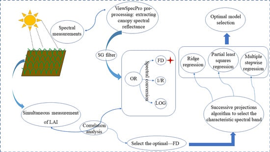
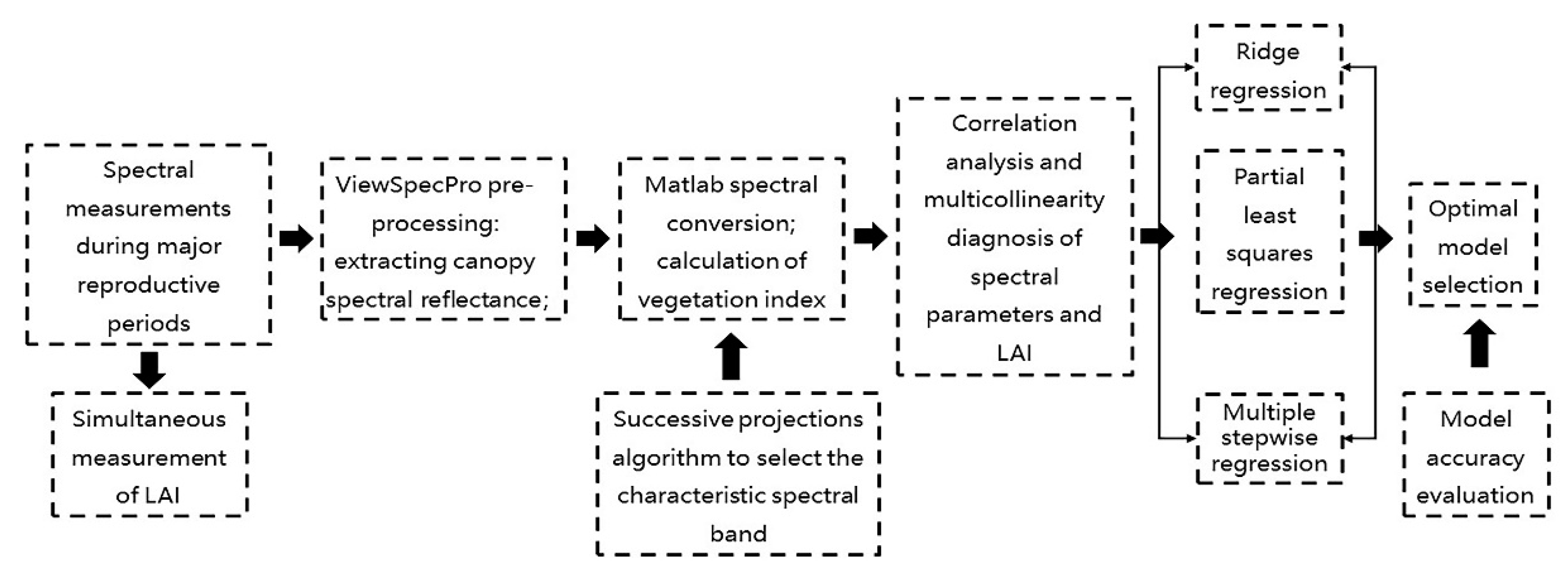
2. Materials and Methods

As shown in Figure 1. This was a flowchart of the entire study, and the approach used had four main stages: data collection and processing, multicollinearity diagnosis, model build, and model validation. A detailed description of the steps was given in Section 2.1, Section 2.2, Section 2.3, Section 2.4, Section 2.5, Section 2.6 and Section 2.7.

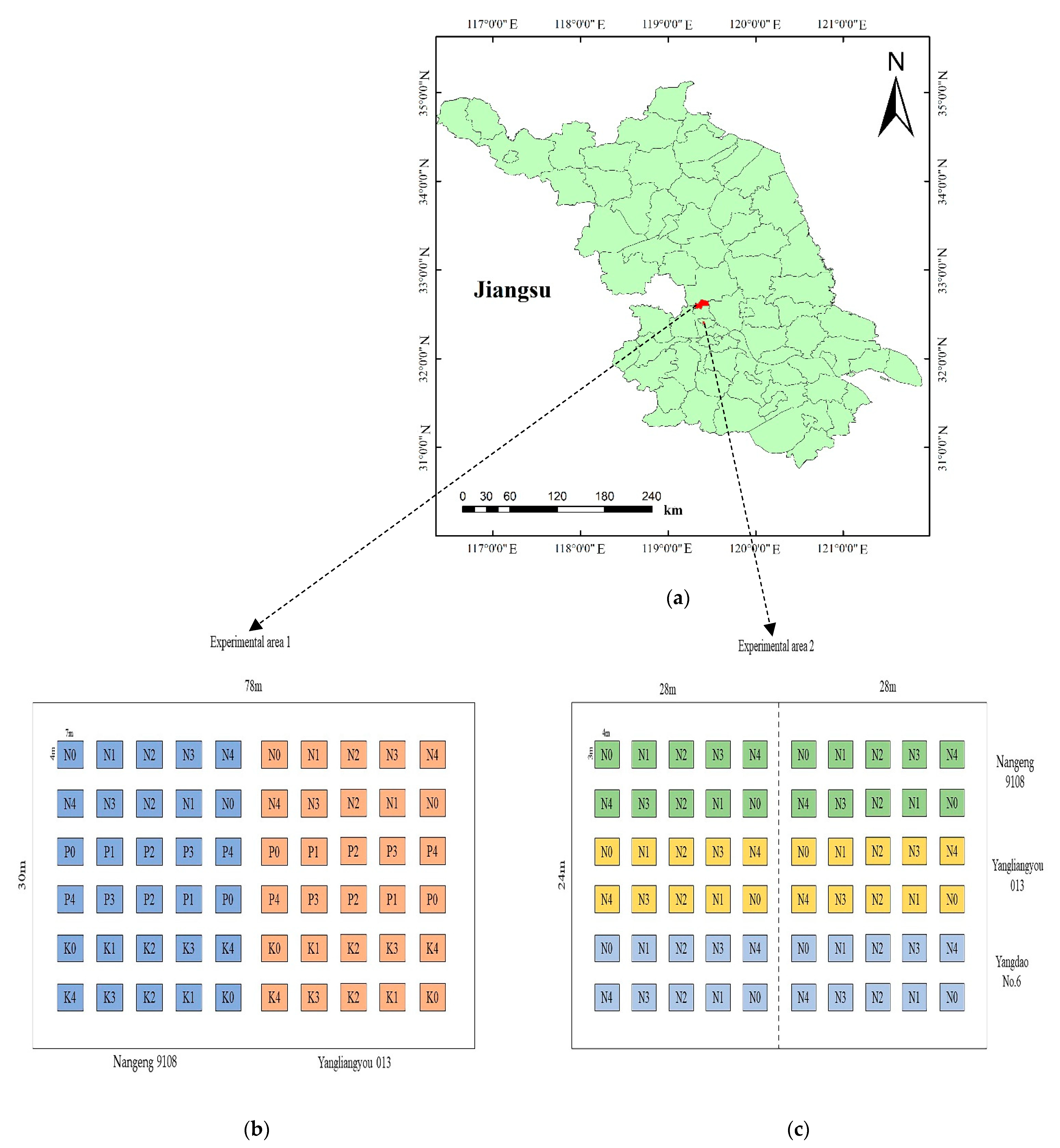
2.1. Experimental Design

The experiment site 1 was set up at the test field in Gongdao Town, Yangzhou City, Jiangsu Province, China, in 2019. The experimental locations were marked in Figure 2a. The experimental cultivars were Nangeng 9108 and Yangliangyou 013, each with 5 nitrogen (N) fertilizer levels (0, 100, 200, 300, and 400 Kg ha−1), 5 potassium (K) fertilizer levels (0, 50, 100, 150, and 200 Kg ha−1), and 5 phosphorus (P) fertilizer levels (0, 100, 200, 300, and 400 Kg ha−1). The experiment adopted randomized block design with a total of 60 plots. The specific distribution was shown in Figure 2b.
The experiment site 2 was set up at the Yangzhou University test base, Jiangsu Province, China. The field experiment was a continuous experiment in 2015 and 2016. The experiment was set up as 3 different experimental varieties (Nangeng 9108, Yangliangyou 013 and Yangdao No.6) using the same fertilizer gradient, with a total of 60 plots. The specific distribution was shown in Figure 2c.
Both experimental sites were located in Yangzhou, China, which was situated at the southern end of the Jianghuai Plain and was influenced by the monsoon circulation, with four distinct seasons, mild climate, and superior natural conditions. The average annual temperature was 14.8 °C, and the annual precipitation was 961~1048 mm. The organic matter and fast-acting phosphorus content of soil nutrients in arable land were generally at a moderate to low level, and the fast-acting potassium content was at a moderate level.

2.2. Data Collection

A total of four characteristic fertility stages of rice were selected for spectroscopy in the experiment: elongation stage (13 August 2019), booting stage (21 August 2019), heading stage (8 September 2019), and post-flowering stage (25 September 2019). Canopy spectra, which were draped spectra, were obtained using a Fieldspec®3 (350–2500 nm) Hi-Res type spectrometer from ASD (Analytical Spectral Devices, Inc., Boulder, CO, USA), with sampling intervals of 1.3 nm (in the 350–1000 nm interval) and 2 nm (in the 1000–2500 nm interval). The ASD had a spectral resolution of 3 nm at 700 nm, 8.5 nm at 1400 nm, and 6.5 nm at 2100 nm. Spectra were measured in clear weather with no wind or very low wind speed between 10:30 and 14:00 BST. Three rice plants of similar growth were selected for spectral measurements in each treatment, and each measurement was repeated five times. Before each measurement, the sensor needs to be finely calibrated using a standard white reflectance panel (the standard white panel reflectance is 1), and the sensor probe was placed vertically 60 cm above the rice plant after the calibration was completed. The data measured by the spectrometer were converted to raw spectral reflectance data using View Spec Pro software after the measurement, and Excel 2019 averaged the repeated measurements as the reflectance spectral values of the measurement points.
At the elongation stage (13 August 2019), booting stage (21 August 2019), heading stage (8 September 2019), and post-flowering stage (25 September 2019) of rice, the aboveground plant parts at the experimental sites were collected, packed in sampling bags, with sampling point information marked on the outside of the sampling bags. The samples were transported to the laboratory in time. Select rice in good growth condition (10 leaves per rice plant were randomly selected and each leaf was measured three times), measure the total width of its leaves with a CI-203 (CID USA, Inc., Bethesda, MD, USA) leaf area meter, then cut the sample section from the middle of the leaf, and bake the sample section and the remaining leaves at 80 °C for more than 48 h to reach a constant weight. Their weights were measured, and the LAI of each sampling point was calculated using the dry weight method, and the average value of five identical sampling points was used as the LAI measurement for that sampling point.
L e a f   a r e a   p e r   u n i t   w e i g h t ( cm 2 . g 1 )   = T o t a l   l e a f   w i d t h   o f   s a m p l e   s e g m e n t × S a m p l e   s e c t i o n   l e n g t h S a m p l e   s e c t i o n   d r y   w e i g h t
T o t a l   s a m p l e   r i c e   l e a f   a r e a = L e a f   a r e a   p e r   u n i t   w e i g h t × T o t a l   s a m p l e   p l a n t   l e a f   d r y   w e i g h t
A v e r a g e   l e a f   a r e a   p e r   r i c e ( cm 2 ) = T o t a l   s a m p l e   r i c e   l e a f   a r e a N u m b e r   o f   s a m p l e   r i c e
In this study, Gongdao data for 2019 were measured spectrally at the elongation, booting stage, heading, and post-flowering stages, and the corresponding rice leaves would be picked on the day of spectral measurement to calculate LAI. The measured spectral data were exported with View Spec Pro (Analytical Spectral Devices, Inc., Boulder, CO, USA), smoothed, and vegetation indices were calculated. For the validation data from 2015–2016, the operational steps for measuring the data were consistent.

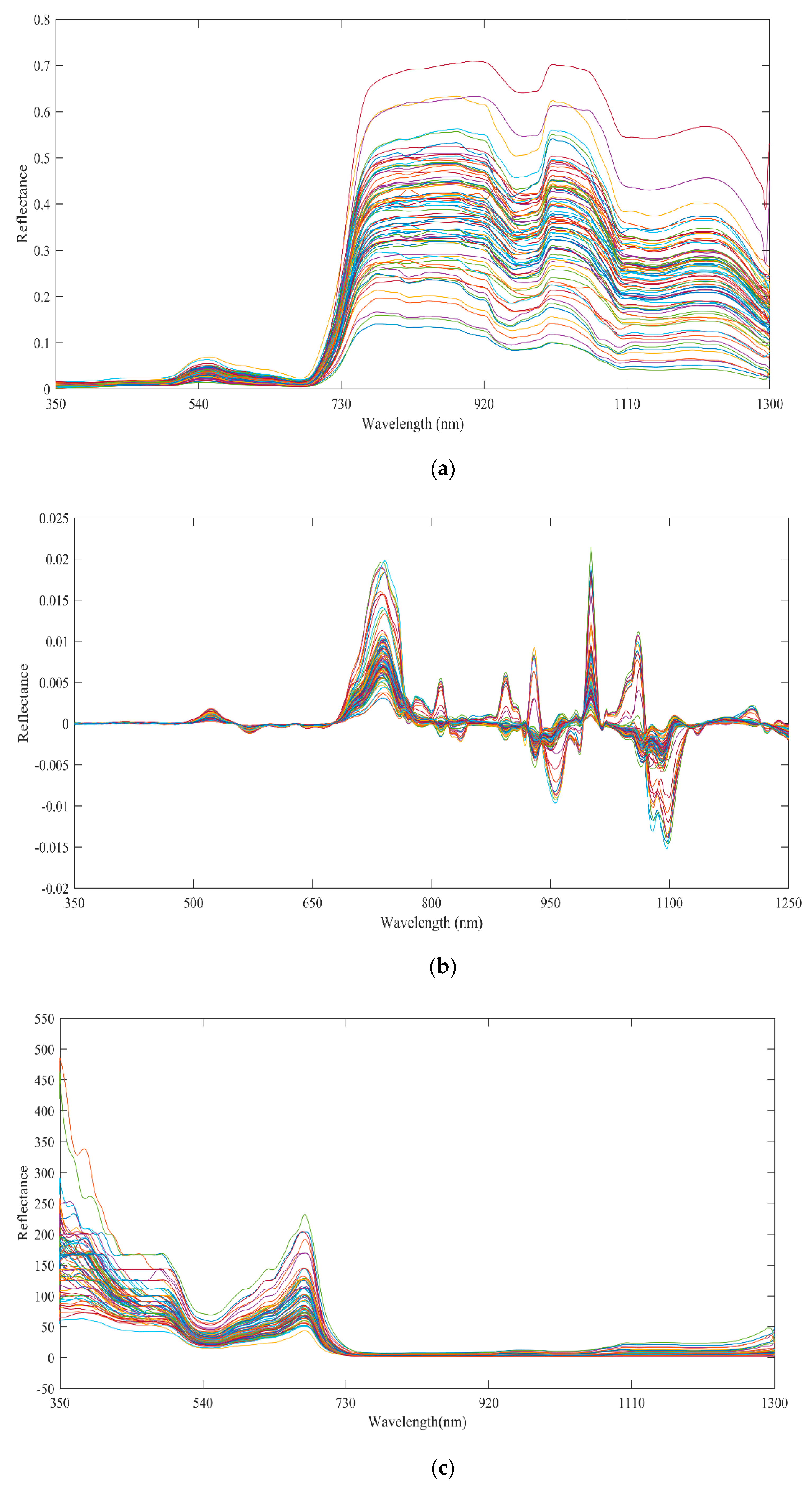
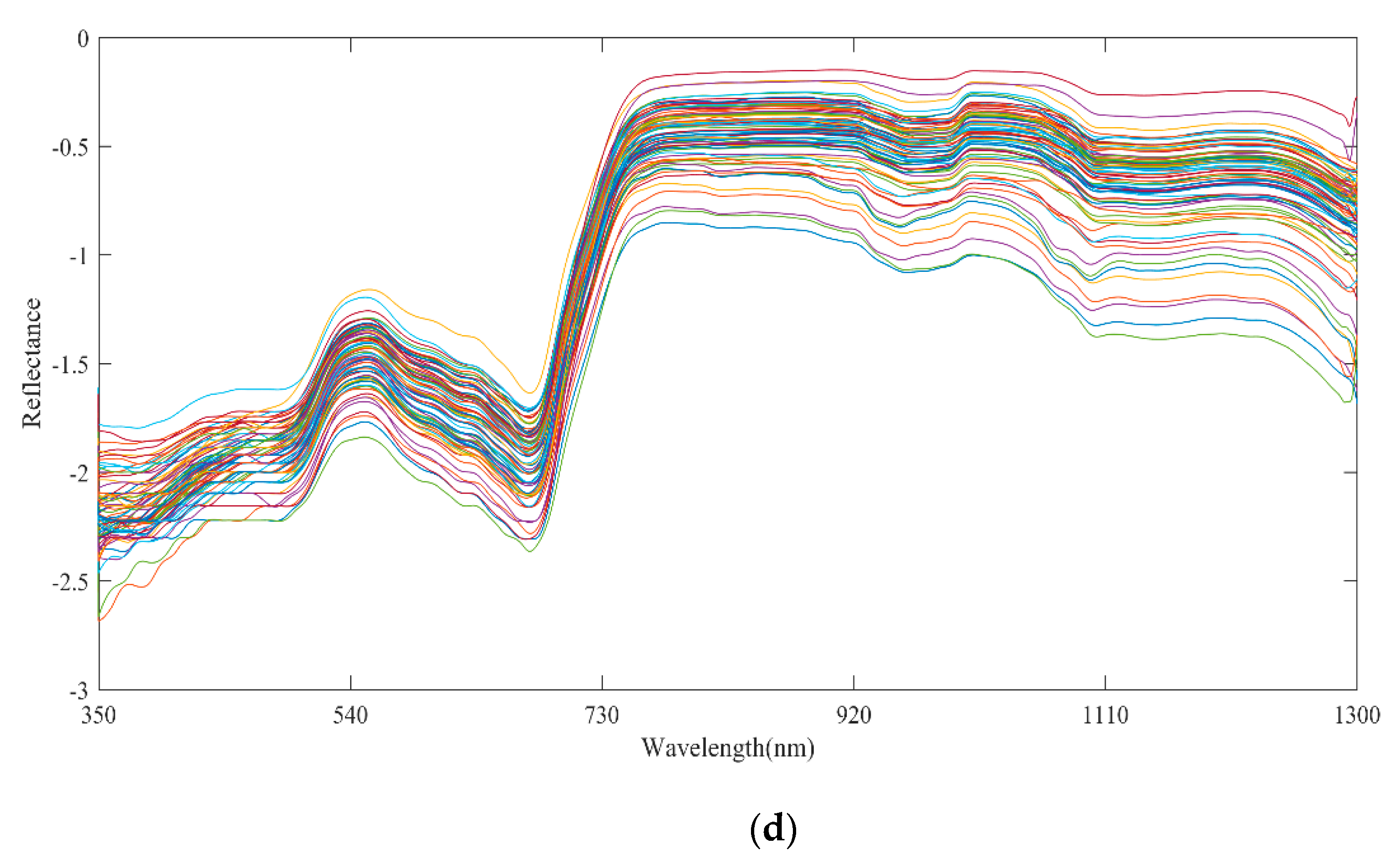
2.3. Hyperspectral Data Preprocessing

The hyperspectral data had a large noise at multiple wavelengths in the range of 350~2500 nm, in order to eliminate the effect of light scattering and noise for a more realistic representation of the spectral characteristics of ground objects. Therefore, a smoothing filtering ground approach was chosen to pre-process the spectra [17,18]. Additionally, in this study, the Savitzky–Golay (SG) convolution smoothing algorithm was used, which was an improvement of the moving average algorithm [19,20]. Smoothing by the SG filter may improve the smoothness of the spectrum and reduce the interference of noise. The effect of the SG smoothing filter varied with the selected value of the window length, meeting the needs of various occasions.
The filter window length was set at n = 2 m + 1 and the measurement points were x = ( m , m + 1 ,   ,   0 ,   1 , , m 1 , m ) . k 1 order of polynomial was used to fit the data in the window:
y = a 0 + a 1 x + a 2 x 2 + a k 1 x k 1
If the system of equations had a solution, n should be larger than or equal to k . Usually, n > k was used. The fitting parameter A was determined by the least-squares fitting, which was expressed as a matrix:
Y ( 2 m + 1 ) × 1 = X ( 2 m + 1 ) × k · A K × 1 + E ( 2 m + 1 ) × 1
The least-squares solution of A was:
A ¯ = ( X T X ) 1 X T Y
The model predicted or filtered value of Y was:
Y ¯ = X A = X ( X T X ) 1 X T Y
The raw canopy spectra (measured during the four main fertility periods) were first exported by View Spec Pro, then the raw canopy spectra were smoothed using the SG filter in Matlab version 2016b, and the processed spectra were labeled as raw reflectance (OR), after which three spectral transformations (all based on OR) were performed to extract useful information. The spectra obtained by the first derivative transform were noted as First-derivative (FD). Similarly, we had the spectrum after reciprocal transformation (1/R), and after logarithmic transformation (LOG).

2.4. Method for Characteristic Bands Selection

The band data of hyperspectral were cumbersome (containing 350 nm–2500 nm), and if all of these bands were modeled, redundant information would occur, so the selection of sensitive bands became critical [21]. In this study, two methods were used to extract sensitive bands, a successive projections algorithm and a Pearson correlation.
SPA was a forward variable selection algorithm that minimizes the variable collinearity of the vector space [22,23]. The characteristic variables were selected by calculating the projection vector size of the remaining variables and the selected variables, so as to ensure the minimal linear relationship between the selected variables. It could eliminate the redundant information in the original spectral matrix, and was often used for the characteristic spectral wavelength screening. In this study, Matlab 2016b version was used to iteratively train SPA. SPA was a forward iterative search method that started with a wavelength, and then added a new variable in each iteration until the number of selected variables reached a set value. The specific process is shown in Algorithm 1 [24]. SPA was used to extract the characteristic bands with the highest correlations between canopy spectrum and LAI, in seeking to improve the accuracy of the established model.
P x j = x j ( x j T x k ( n 1 ) ) x k ( n 1 ) ( x k ( n 1 ) T x k ( n 1 ) ) 1
Let x j be the jth column of the calibration set spectrum such that x j = P x j , then let n = n + 1, and so on for the calculation.
Algorithm 1: SPA
Input: Analysis   of   the   spectrum X ,   initial   band   k ( 0 ) ,   number   of   selected   variables   N .
Step 1: Initialization :   n = 1 ; x j X j ,   j = 1 , 2 , , J ;
Step 2: S = { X i , 1 i J , i { k ( 0 ) , , k ( N 1 ) } } , Determine the unselected band variable.
Step 3:Calculate the projection mapping of the unselected and initialized bands:
P x j = x j ( x j T x k ( n 1 ) ) x k ( n 1 ) ( x k ( n 1 ) T x k ( n 1 ) ) 1
Step 4:Determine the maximum projection: k ( n ) = m a x ( || P x j || ) , x j S ;
Step 5: x j = P x j , j S ;
Step 6: n = n + 1 ,   when   n < N , return to step 2;
Step 7: Determine   the   selection   of   the   band   sequence :   { k ( n ) ; n = 0 , , N 1 } ;
Output:Selected band.
Pearson correlation was a way to measure the correlation between two variables, and the correlation was generally judged by the magnitude of its coefficient [25]. In this study, we modeled LAI with canopy spectral bands by Pearson correlation analysis using SPSS25, and selected ten bands with high correlation and relative dispersion as sensitive bands. The purpose was to compare the accuracy with the model built from the sensitive bands extracted by SPA.

2.5. Method for Vegetation Indices Selection

According to previous studies [21,26,27], a large number of vegetation indices were used to monitor the growth of crops. In this study, OR was used to calculate the vegetation index, and wave averaging was used to reduce errors and improve the generalizability of the application. The calculated vegetation indices were correlated with LAI, and the following six vegetation indices were selected as highly significant (p < 0.01). The calculation equations are listed in Table 1. The purpose of introducing the vegetation index was to model with the screened characteristic bands and then compare with the later model without the vegetation index.

2.6. Model Development

2.6.1. Multicollinearity Diagnosis

Multicollinearity was a phenomenon in that the established model was inaccurate and distorted due to strong correlations between the independent variables for modeling. Ordinary linear regression models could not satisfy the fit in the presence of multicollinearity, nor could they truly reflect the effect of independent variables on the dependent variable indicators [34].
The variance inflation factor ( V I F ) was a way to determine the presence of multicollinearity by examining the extent to which a given explanatory variable was explained by all other explanatory variables in the equation. Each explanatory variable in the equation had a VIF, which reflected the extent to which the multicollinearity increased the variance of the estimated coefficients [35]. The variance expansion factor was defined as [36]:
V I F = ( 1 R 2 ) 1
In the above equation, R 2 was the coefficient of determination of this independent variable on the other independent variables of relevance.
Although there the VIF did not have a fixed upper limit, it was generally judged to have multicollinearity if it exceeded 10 [35].

2.6.2. Modeling Methods

Ridge regression was a commonly used regularization method. It solved the issue of multicollinearity of independent variables in linear regression by reducing the accuracy and deleting some information including noise to establish an optimal model [37]. The biggest difference between the ridge regression and the least-squares method was that in ridge regression, the unbiasedness was slightly abandoned but the stability was improved. The cost function of ridge regression was:
J ( θ ) = 1 2 m [ i = 1 m ( h θ ( x ( i ) ) y ( i ) ) 2 + λ j = 1 n θ j 2 ]
where   j = 1 n θ j 2 represented the penalty coefficient, λ was the ridge parameter, i = 1 m ( h θ ( x ( i ) ) y ( i ) ) 2   was the residual sum of squares (RSS) of the original multiple linear regression.
Partial least squares regression was a statistical method that was related to principal component regression [38]. However, instead of finding the hyperplane with the largest variance between the dependent variable and the independent variable, it projected the dependent variables and independent variables, respectively, into a new space to search for a linear regression model [39]. PLS could achieve the maximum extraction of information reflecting data changes.
Multiple stepwise regression was a method to automatically select the most important variables from a large number of optional variables to establish a predictive or explanatory model for regression analysis [40,41]. The selection of variables was based on the impacts of the independent variables on the dependent variables, adding the variables with large impacts and removing the variables with small impacts.
A multiple linear regression model with multiple parameters was established by multiple stepwise regression. The equation for this type of model was:
y = b 0 + b 1 x 1 + b 2 x 2 + b n x n + e
where y was the dependent variable, x 1 ,   x 2 , , x n   were the n independent variables used in modeling, b 0 , b 1 , b 2 , , b n were the constant terms corresponding to each independent variable, and e was the error term.
These three models were used because they have the ability to eliminate multicollinearity between independent variables. In this study, all three models mentioned above were modeled with selected characteristic spectral wavelengths and vegetation indices as independent variables, and LAI as dependent variables. The three models were chosen to compare which model has higher accuracy and better for monitoring rice LAI.

2.7. Model Evaluation

In this study, SPA was used to extract the optimal bands related to rice LAI, and then RR, PLS, and MSR were used to build the rice LAI model. The data were analyzed with EXCEL19, SPSS25 (Statistical Product and Service Solutions), and Matlab 2016b. The plots were made with GraphPad Prism, Arcgis 10.6, and Matlab 2016b.
A portion of the measured data (n = 60) from the 2019 Gongdao was used as the training set, the remaining data (n = 60) as the validation set 1, and the test base data (n = 60) from 2015 to 2016 from Yangzhou University as the validation set 2. The model evaluation metrics were the coefficient of determination ( R 2 ) and the root-mean-square error ( R M S E ).
R M S E = 1 n 1 i = 1 n ( y i y j ) 2
where y i was the measured value, y j was the predicted value, and n was the sample size.
R 2 = 1 i = 1 m ( y i y ^ i ) 2 / i = 1 m ( y i y ¯ ) 2
where y i and y ^ i were the actual value and predicted value of the ith sample, respectively, and the average value y ¯ = 1 m i = 1 m y i .

3. Results

3.1. Spectral Preprocessing

The canopy spectral curves of all rice samples across the whole growth stages were processed by SG filter. The processed results (OR) were shown in Figure 3a. The canopy spectral curve of rice was between 0 and 0.8, and the region 1300−2500 nm with large fluctuation due to noise was truncated. In the region of 700−800 nm, the canopy spectral reflectance increased rapidly. In the region of 800−900 nm, the reflectance was stable. In the 950 nm region, there was a short drop point, and then it increased steadily. The reflectance was decreasing beyond 1100 nm.
The results of the first–derivative (FD) processing were shown in Figure 3b. The canopy spectral reflectance of rice ranged from −0.02 to 0.025, and the 1250−2500 nm region with large fluctuations due to noise was truncated. The first peak was reached in the region of 670−750 nm, followed by a continuous small-scale float in the region of 750 nm−1000 nm and three consecutive peaks at 1000−1150 nm with more obvious changes, and the curve leveled off after 1150 nm.
The results of the reciprocal (1/R) processing were shown in Figure 3c. The canopy spectral reflectance of rice ranged from −50 to 550, with a more pronounced decrease at 350–540 nm, followed by the first peak at 540–730 nm, with a peak reflectance close to 250, and finally leveling off at 730–1300 nm.
The results of the logarithmic (LOG) processing were shown in Figure 3d. The canopy spectral reflectance of rice ranged from −3 to 0, with the first peak at 350–700 nm (close to −1.1), followed by a gradual increase at 700−760 nm, and finally a leveling off at 760–1300 nm.
This indicated that FD could effectively extend the effective spectrum and lay the foundation for further studies to follow.

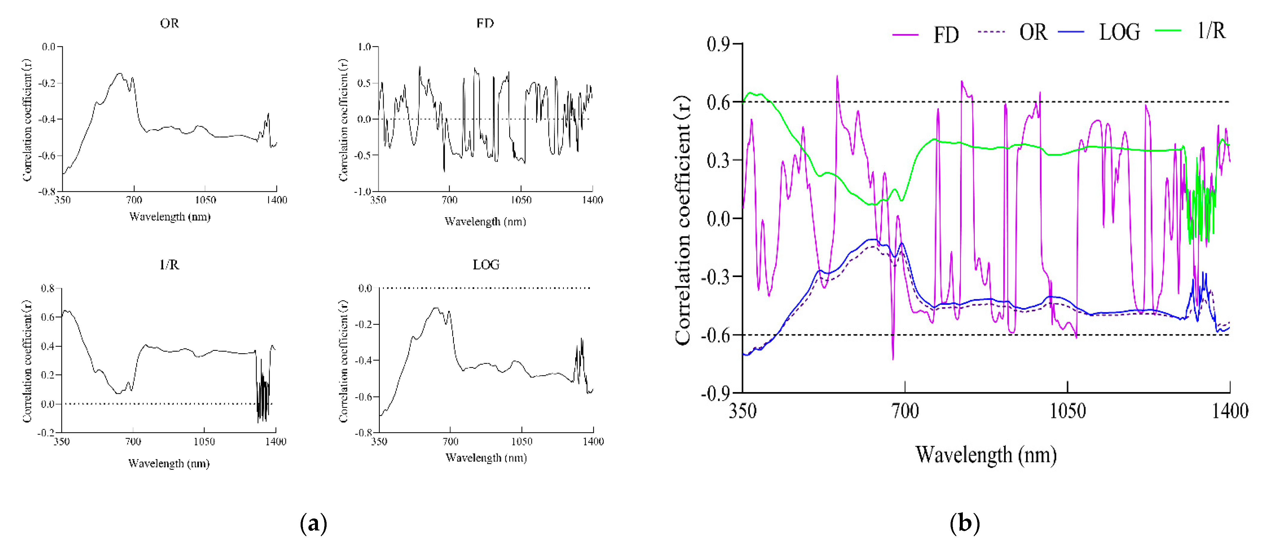
3.2. Correlations between Rice Canopy Spectral Transformations and LAI

To better compare the impacts of spectral transformations on LAI, based on the original reflectance (OR), three transformations, FD, LOG, and 1/R were conducted and their correlations with LAI were investigated. It could be seen from Figure 4a that the correlation of OR with LAI was increasing in the wavelength range of 350−700 nm, with the strongest correlation coefficient of −0.702. The correlation was decreasing in the range of 700−1400 nm, approaching −0.5. The correlation curve of FD exhibited continuous fluctuations with multiple peaks, extending the sensitive bands with better correlations, reaching the highest peak at 544 nm with a correlation coefficient of 0.733. The overall effect of FD was better than OR. The correlation curve of LOG was similar to that of OR, with the strongest correlation coefficient of −0.704, not significantly improved compared with OR. The correlation curve of 1/R first decreased and then increased, giving a maximum correlation coefficient in the range of 350−700 nm (r = 0.646). It tended to be flat in the range of 750−1300 nm, with a correlation coefficient close to 0.4.
Figure 4b was made based on the above analysis. The function curve of y = |0.6| was added as a reference to compare the fluctuation ranges of the four preprocessing correlation curves. It was concluded that FD > OR > LOG > 1/R. Therefore, FD processing was selected as SPA input for characteristic bands.

3.3. Screening of Characteristic Bands

The advantage of SPA was that it extracted several characteristic wavelengths of the full range, eliminating redundant information in the original spectral matrix and preventing overfitting during modeling. As shown in Figure 5, the iterative selection of the spectra processed by SPA for OR and FD showed that, under the same number of iterations, the number of characteristic bands selected by the original spectrum was larger, but relatively concentrated at 1230–1400 nm. The first−derivative spectrum could effectively reduce the concentrated distribution of feature bands. This indicated that the first−derivative processed spectral bands could be validly extended, which was conducive to obtaining the optimal bands. Therefore, the choice of first−derivative spectra as the characteristic band made the selection feasible.
The canopy spectra processed by FD across all the growth stages were firstly smoothed for the second round by the SG filter. Then, the characteristic bands were obtained by iterative training. It could be seen from Figure 5c,d that with a variable number of 35, the RMSE was 1.096, and 35 characteristic bands were preferably selected. These characteristic bands were screened out, and 10 characteristic bands with long distances were selected from them to reduce the probability of collinearity, preparing for model optimization.
Then, 10 bands with the highest Pearson correlations were selected and compared with those from SPA, in order to check whether the sensitive bands selected by SPA were superior. The selection results of the two methods are listed in Table 2.

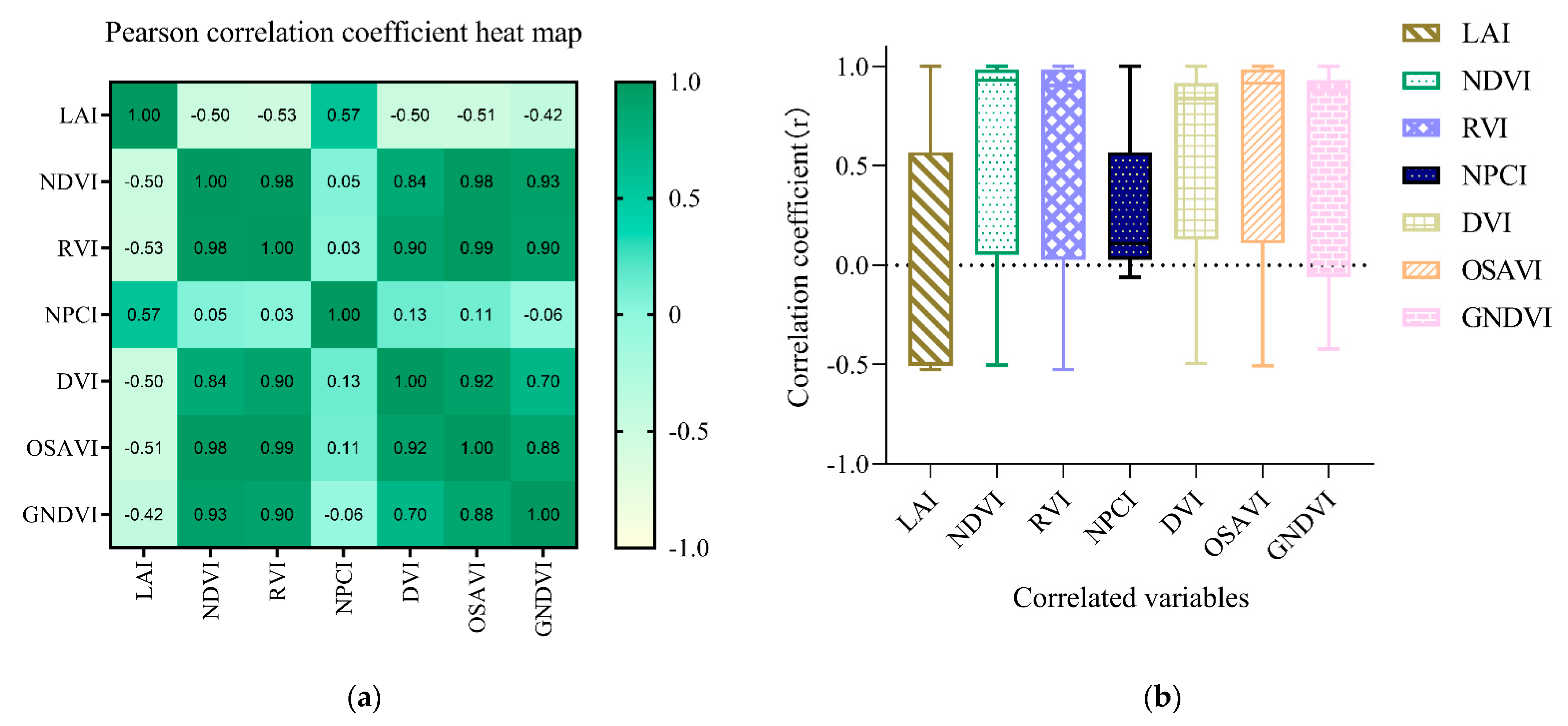
3.4. Determination of Multicollinearity

Due to the continuity of the bands, theoretically multicollinearity occurs. Now, the selected vegetation indices were subjected to Pearson analysis. Then, the characteristic bands and vegetation indices of the whole growth stage were taken to variance inflation factor (VIF) test on the relevant independent variables to determine multicollinearity.
Correlation analysis was carried out between vegetation indices and LAI regarding the whole growth stage, and Pearson correlation coefficient heat map and box-and-whisker plot were made. As shown in the heat map of Figure 6a, the correlation between NPCI and LAI was the highest (r = 0.568, p < 0.01), followed by RVI (r = −0.526, p < 0.01). The correlations were in the order of NPCI > RVI > OSAVI > NDVI > DVI > GNDVI. Therefore, NPCI could serve as one of the independent variables for modeling.
In addition to the correlation between the selected vegetation indices and LAI, there were also strong correlations between individual vegetation indices. As shown in the box-and-whisker plot of Figure 6b, the correlation was 0.980 between NDVI and OSAVI, was 0.980 between NDVI and RVI, and was 0.920 between OSAVI and DVI. VIF test on these parameters was performed.
As shown in Table 3, in terms of vegetation indices, all the vegetation indices showed strong covariance except for NPCI (VIF = 1.373) and GNDVI (VIF = 9.783) which had no collinearity. Regarding the characteristic bands, among those selected by Pearson correlation, all bands had strong collinearity except for 675 (VIF = 3.972) nm. While the characteristic bands processed by SPA had significantly decreased collinearity compared with the Pearson correlation. Though the collinearity was not totally eliminated, the VIF output was significantly optimized.

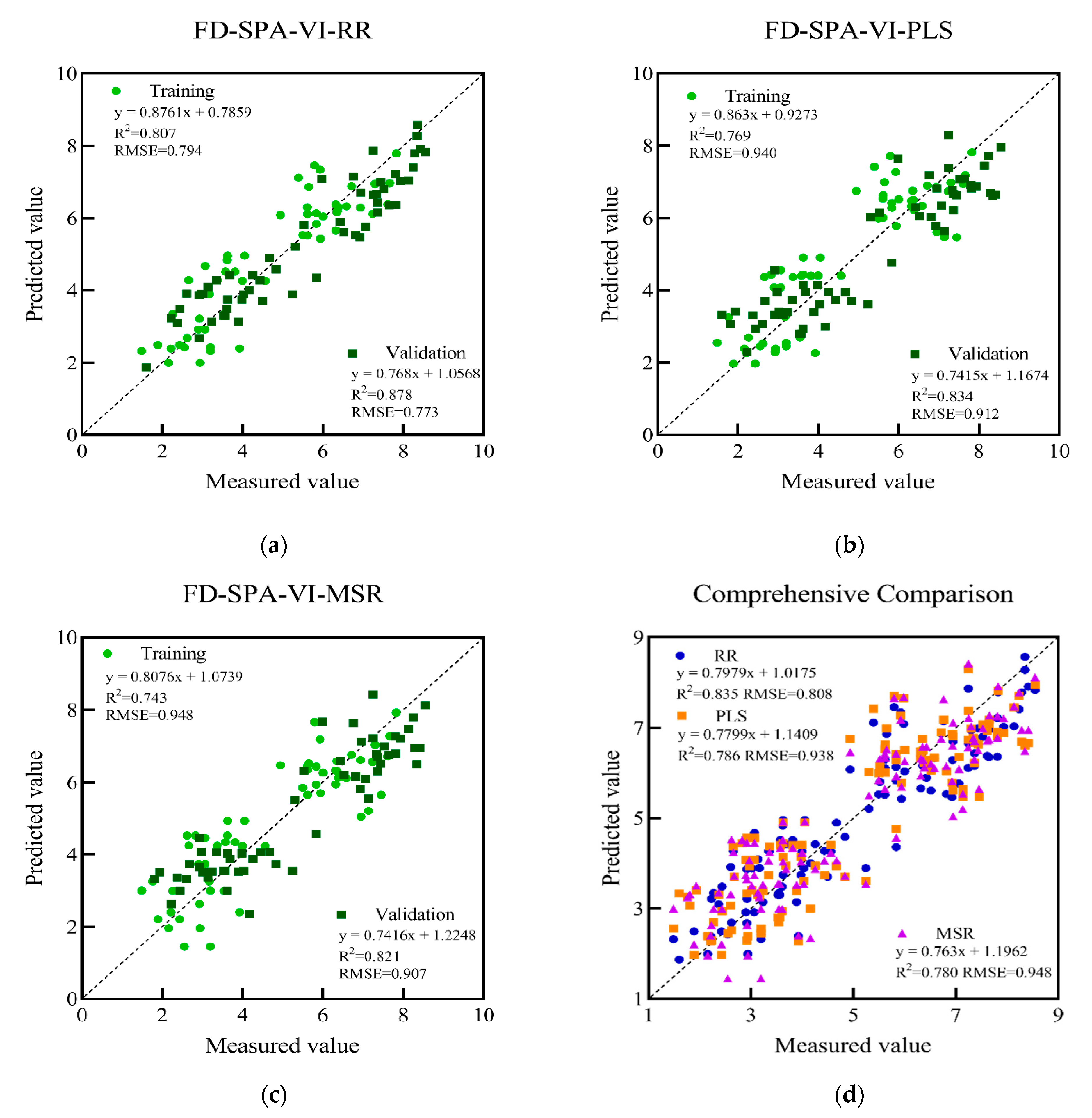
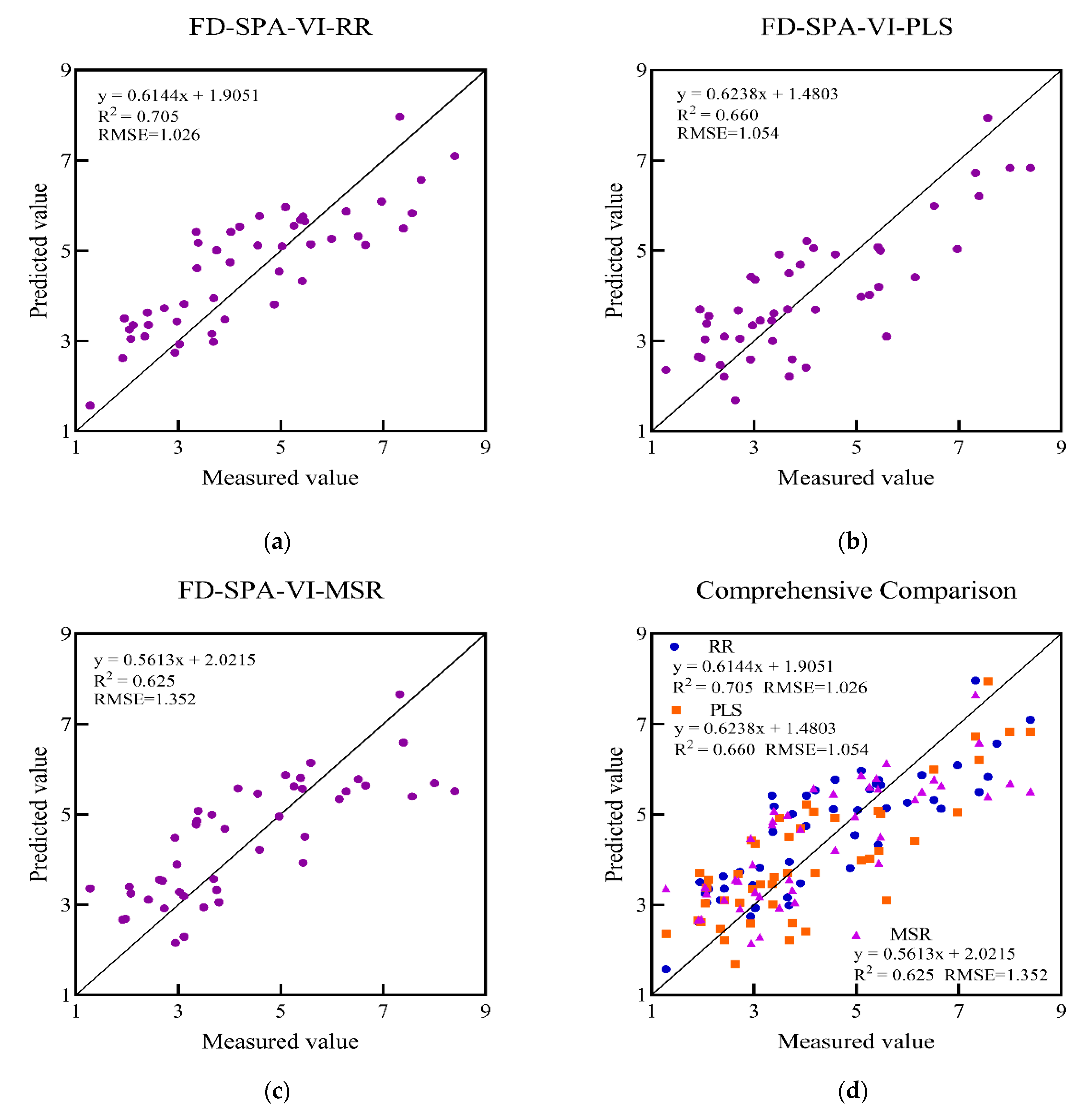
3.5. Establishment and Evaluation of LAI Estimation Model

The characteristic bands were extracted on FD using the SPA and Pearson correlation, respectively. The respective extracted bands were modeled with the LAI in three ways (RR, PLS, MSR) in order to compare which modeling method was more superior and which feature band extraction method had higher model accuracy. Additionally, the model evaluation metrics were R2 and RMSE.
As shown in Table 4, without the inclusion of vegetation index (VI), either using SPA or Pearson correlation, the characteristic bands they chose to model with LAI were modeled best with RR, with the R2 of 0.718 and RMSE of 1.071 for FD-SPA-RR and the R2 of 0.706 and RMSE of 1.067 for FD-Pearson-RR. Comparing the characteristic bands selected by these two methods (SPA, Pearson) separately, it could be seen that the characteristic bands selected by SPA were better modeled with the three models (RR, PLS, MSR) than Pearson.
Comparing again with the addition of vegetation index, FD-SPA-VI was first compared with FD-Pearson-VI, and the better modeling of the characteristic bands selected by SPA was still obtained, which led to the conclusion that SPA was better than Pearson in selecting the characteristic band. Then, the three models of FD-SPA-VI were compared synthetically to conclude that the accuracy of ridge regression is higher, with R2 of 0.807 and RMSE of 0.794 for FD-SPA-VI-RR.
Finally, FD-SPA was compared with FD-SPA-VI, and the table revealed that the accuracy of the model with vegetation index was generally higher than that without VI. The R2 of FD-SPA-RR was 0.718 and the RMSE was 1.071, and the R2 of FD-SPA-VI-RR was 0.807 and the RMSE was 0.794.
In summary: (i). The modeling accuracy of the characteristic bands selected by SPA was higher than that of Pearson correlation; (ii). Among the three modeling methods, ridge regression was the best; (iii). The inclusion of vegetation index could significantly improve the model accuracy.
To further verify whether the model of FD-SPA-VI-RR performed superior, the two ways using SPA were compared on the validation sets.
As shown in Table 5, the performance of the FD-SPA-VI model was indeed superior to that of characteristic bands alone (FD-SPA). The R2 of the FD-SPA-VI-RR model using the validation sets was increased by 0.071 compared with using the training set, and RMSE was decreased by 0.021. The R2 of the FD-SPA-VI-PLS model using the validation sets was increased by 0.065 compared with using the training set, and RMSE was decreased by 0.028. The R2 of the FD-SPA-VI-MSR model using the validation sets was increased by 0.078 compared with using the training set, and RMSE was decreased by 0.041. In conclusion, FD-SPA-VI-RR was more predictive for LAI. The above conclusion was correct.
As shown in Figure 7, the fit of the characteristic bands to the vegetation index was excellent and the modeling results were accurate, indicating that SPA was effective in selecting characteristic bands. Comparing the models of the three modeling sets together, the RR model improved R2 by 0.038 and reduced RMSE by 0.146 compared to the PLS model, and improved R2 by 0.064 and reduced RMSE by 0.154 compared to the MSR model. The modeling of RR performed better than that of PLS and MSR. Comparing three validation sets, the RR model improved R2 by 0.044 and reduced RMSE by 0.139 compared to the PLS model, and improved R2 by 0.057 and reduced RMSE by 0.134 compared to the MSR model. The R2 and RMSE of the validation set generally performed better than that of the modeling set, indicating that all three models were able to eliminate the overfitting problem, but the RR model was superior in monitoring the LAI.
In addition, the accuracy with VI introduced was elevated compared to without VI. Therefore, the FD-SPA-VI-RR model could be used to effectively monitor the LAI of rice.
Thus, the optimal model for monitoring LAI was:
LAI = 5.827 − 67.493 × R752 + 594.376 × R913 + 412.731 × R984 − 233.567 × R1044 − 9.811 × R1097 + 139.265 × R1278 + 67.214 × R1295 − 3.233 × R1303 − 6.272 × R1347 + 26.163 × R1371 + 9.394 × NPCI.
To verify whether different varieties and different nitrogen fertilizer levels may affect the prediction accuracy of the model, this study adopted completely independent validation sets to re-evaluate the optimal model based on FD-SPA-VI. The evaluation results are shown in Figure 8. As shown, the model based on FD-SPA-VI-RR was significantly better than the other two in terms of both R2 and RMSE due to the influence of the whole growth stage. The FD-SPA-VI-RR model can achieve R2 of 0.705 and RMSE of 1.026 for the validation set. Comparing the three models together, the RR model improved R2 by 0.045 and reduced RMSE by 0.028 compared to the PLS model, and improved R2 by 0.080 and reduced RMSE by 0.326 compared to the MSR model. Therefore, the optimal model for predicting rice LAI was the one based on FD-SPA-VI-RR.

4. Discussion

After reviewing the results of previous studies, it was proved that hyperspectral could obtain the spectral information of crops and analyze the reflectance of crops without destroying the vegetation [42]. LAI was an important parameter to characterize crop growth and predict crop biomass, the two of which together could quickly and intuitively predict the growth situation of rice [43,44,45]. Therefore, the effective combination of the two had been the focus of research nowadays. Li et al. [46] used fractional differential and continuous wavelet transform to process the hyperspectral reflectance of the wheat canopy, and constructed LAI estimation models for various growth stages. Xing et al. [47] studied the vegetation indices and their optimized red-edge modified counterparts to retrieve the LAI for five main growth stages, and used hyperspectral data to analyze the relationship between the LAI and the vegetation indices. Some scholars have also combined ground hyperspectral data with satellite remote sensing to monitor the growth of crops on the ground. For example, Chen et al. [48] used China GaoFen-5 (GF-5) hyperspectral data to estimate LAI using different feature selection and machine learning methods. However, the combination of these two was based on the original spectrum, and no spectrum transformation was performed. Therefore, it was unknown whether the model after spectrum conversion would be superior to the original spectrum. In the present study, based on the preprocessing of the original spectrum by the SG convolution smoothing method, the first-derivative transformation, the reciprocal transformation and the logarithmic transformation were conducted [49]. Furthermore, the correlations between the four types of spectra and LAI were analyzed and compared. It was concluded that compared with the original spectrum, the correlation between FD and LAI was higher and FD effectively extended the sensitive bands with higher correlations, convenient for the screening of subsequent characteristic bands.
In terms of the selection of characteristic bands, some scholars extracted the optimal bands through the correlations between the spectral bands and the independent variables. Liu et al. [50] selected the characteristic bands of chlorophyll content by introducing an improved ant colony optimization with an automatic updating mechanism (AU-ACO), and compared it with standard ACO algorithm and full-band modeling methods. Guo et al. [51] used the continuum removal method to expand the characteristic bands of the absorption spectrum of chlorophylls. The convergence speed of the ant colony algorithm was slow, and it was easy to cause local optimal solutions. Moreover, the selection of parameters relies more on experience and trial and error, and inappropriate initial parameters will weaken the algorithm’s ability to find the optimum. Now, the iterative optimization of SPA can be applied to the selection of hyperspectral characteristic bands (Xie et al. [52]), and the advantage of the successive projections algorithm (SPA) was that it was faster, more accurate, and easier to implement than the ant colony algorithm, and facilitates the elimination of redundant information in the original spectrum matrix [13]. Overfitting of the model was the most feared problem in most studies. In this study, SPA and Pearson correlation were used to extract the FD-processed canopy spectrum. The comparison between these two methods indicated that SPA was superior in extracting the spectrum bands. It not only improved the accuracy, but also eliminated the problem of overfitting.
In terms of modeling methods, when multicollinearity existed in the selected correlated independent variables, there were three methods to eliminate collinearity: ridge regression, principal component analysis (PCA), and partial least squares. PCA and PLS have been widely applied. Kleshchenko et al. [53] used PCA to calculate the dependence equation of winter wheat yield on extracted components. Peron Danaher et al. [54] used a spectroradiometer combined with leaf tissue to collect the spectral profiles of wheat leaves and canopies for standard analysis and determination of nitrogen, and then established prediction models for leaf and canopy nitrogen concentrations using PLS regression. Agricultural application of ridge regression was not as popular as the other two, but it did not mean that the model accuracy of ridge regression was lower. Ahmed A et al. [55] used the kernel ridge regression (KRR) method with complete ensemble empirical mode decomposition with adaptive noise (CEEMDAN) and grey wolf optimization (GWO) to estimate the yield of wheat in South Australia, and the established model had a highly accurate and can be used to support precision agriculture. In this study, a multivariate stepwise regression model was introduced, and further the three modeling methods of RR, PLS, and MSR were compared. Not only a reliable optimal model was obtained, but also the collinearity between the proximity bands was eliminated. The optimal model was FD-SPA-VI-RR, with R2 of 0.807 and RMSE of 0.794.
In addition, the same research base that was used for both training and validation leads to the limitations of the model. In this study, a portion of the data collected in Gongdao Town was used as the training set, the remaining portion of the data was used as the validation set 1, and the data collected at another test site was used as the validation set 2. Two validations were performed as a way to demonstrate whether the selected model had high accuracy. The results showed that the accuracy of the validation set 2 had decreased, but the overall accuracy was higher, and the error had increased. This indicated that the FD-SPA-VI-RR model had a promising application, but more datasets need to be added in the future to ensure the generalizability of the model.
Moreover, this model could also be extended to satellite hyperspectral in the future, which made a fundamental work for monitoring rice LAI, but could not be used directly and required a scale conversion of the band function. Because the optimal model had been found and the model variables were shown, the monitoring of rice LAI could be performed as long as the corresponding band was found in the satellite hyperspectral.
Surely LAI may also be affected by various factors such as climate environment and soil fertility. Therefore, continuous fixed-point experiments were expected that multi-year data could be used in multi-factor analysis, and machine learning could be used for modeling, further improving the model accuracy. Moreover, the correlation between spectral reflectance and LAI was high, but it did not directly indicate that spectral reflectance had a clear indication on LAI. Other factors such as leaf soil plant analysis development (SPAD) need to be considered too. All of these provided a theoretical basis for promoting the monitoring of rice growth.

5. Conclusions

In this study, it was found that the correlation between the rice canopy spectrum after transformation of the original spectrum and LAI was truly improved, with the most distinct improvement occurred for the first-derivative transformation. Therefore, it can be concluded that the first-derivative transformation could enhance the effective information of the spectrum. With respect to the extraction of characteristic bands processed by FD, SPA could accurately and rapidly locate the effective spectral information, effectively improving the accuracy of the subsequent model. SPA had important application value in enhancing model validity and eliminating overfitting problem. Furthermore, introducing vegetation indices with high correlations as independent variables for model establishment may also elevate the model accuracy. Therefore, the optimal modeling combination was FD-SPA-VI-RR, with R2 of 0.807 and RMSE of 0.794 for the training set, R2 of 0.878 and RMSE of 0.773 for the validation set 1, and R2 of 0.705 and RMSE of 1.026 for the validation set 2.
This method was reproducible to some extent. It was not necessary to purchase the same type of sensor with the same specifications, but only the spectrum included in the optimal model proposed in the study, even if it was a simple instrument. If such an instrument was not available in the market, the model also provided a certain technical approach for the independent development of a rice LAI detector, providing a theoretical basis for its application in practical production.
The model was able to be applied to field production because the secondary validation was evaluated with data from Experiment 2, and the accuracy, although reduced, was generally high. In future studies, more sample sizes will be added for model calibration to improve the model and increase its applicability.

Author Contributions

Conceptualization, C.T. and S.J.; methodology, S.J. and C.T.; software, S.J. and C.G.; validation, S.J. and C.G.; formal analysis, S.J., X.X. and H.Z.; investigation, S.J., Q.H., Z.Z. and Z.H.; data curation, S.J.; writing—original draft preparation, S.J.; writing—review and editing, C.T. and S.J.; visualization, S.J. and C.G.; supervision, R.Z. and B.L. All authors have read and agreed to the published version of the manuscript.

Funding

This research was funded by the National Natural Science Foundation of China (No. 32071902), the Key Research Program of Jiangsu Province, China (No. BE2020319), the Yangzhou University Interdisciplinary Research Foundation for Crop Science Discipline of Targeted Support (No. yzuxk202007, No. yzuxk202008) and the Priority Academic Program Development of Jiangsu Higher Education Institutions (PAPD).

Data Availability Statement

Not report any data.

Acknowledgments

The authors are very grateful to remote sensing as a platform to keep us updated with the latest information and intelligence. Finally, we would like to thank our supervisor for providing us with valuable suggestions while writing the article.

Conflicts of Interest

The authors declare no conflict of interest.

References

  1. Yang, K.; Gong, Y.; Fang, S.; Duan, B.; Yuan, N.; Peng, Y.; Wu, X.; Zhu, R. Combining spectral and texture features of UAV images for the remote estimation of rice LAI throughout the entire growing season. Remote Sens. 2021, 13, 3001. [Google Scholar] [CrossRef]
  2. Li, S.; Yuan, F.; Ata-UI-Karim, S.T.; Zheng, H.; Cheng, T.; Liu, X.; Tian, Y.; Zhu, Y.; Cao, W.; Cao, Q. Combining color indices and textures of UAV-based digital imagery for rice LAI estimation. Remote Sens. 2019, 11, 1763. [Google Scholar] [CrossRef] [Green Version]
  3. Yao, Y.; Liu, Q.; Liu, Q.; Li, X. LAI retrieval and uncertainty evaluations for typical row-planted crops at different growth stages. Remote Sens. Environ. 2008, 112, 94–106. [Google Scholar] [CrossRef]
  4. Zhou, H.; Zhou, G.; Song, X.; He, Q. Dynamic characteristics of canopy and vegetation water content during an entire maize growing season in relation to spectral-based indices. Remote Sens. 2022, 14, 584. [Google Scholar] [CrossRef]
  5. Olson, M.B.; Crawford, M.M.; Vyn, T.J. Hyperspectral indices for predicting nitrogen use efficiency in maize hybrids. Remote Sens. 2022, 14, 1721. [Google Scholar] [CrossRef]
  6. Prasad, N.; Semwal, M.; Kalra, A. Hyperspectral vegetation indices offer insights for determining economically optimal time of harvest in Mentha arvensis. Ind. Crops Prod. 2022, 180, 114753. [Google Scholar] [CrossRef]
  7. Yang, R.; Tian, H.; Kan, J. Classification of sugar beets based on hyperspectral and extreme learning machine methods. Appl. Eng. Agric. 2018, 34, 891–897. [Google Scholar] [CrossRef]
  8. El-Hendawy, S.; Al-Suhaibani, N.; Mubushar, M.; Tahir, M.U.; Marey, S.; Refay, Y.; Tola, E. Combining hyperspectral reflectance and multivariate regression models to estimate plant biomass of advanced spring wheat lines in diverse phenological stages under salinity conditions. Appl. Sci. 2022, 12, 1983. [Google Scholar] [CrossRef]
  9. Wang, Z.; Chen, J.; Zhang, J.; Fan, Y.; Cheng, Y.; Wang, B.; Wu, X.; Tan, X.; Tan, T.; Li, S.; et al. Predicting grain yield and protein content using canopy reflectance in maize grown under different water and nitrogen levels. Field Crops Res. 2021, 260, 107988. [Google Scholar] [CrossRef]
  10. Gu, X.; Wang, L.; Song, X.; Xu, X. Estimating Leaf Nitrogen Accumulation in Maize Based on Canopy Hyperspectrum Data. In Proceedings of the Remote Sensing for Agriculture, Ecosystems, and Hydrology XVIII, Edinburgh, UK, 26–29 September 2016. [Google Scholar]
  11. Gao, J.; Ni, J.; Wang, D.; Deng, L.; Li, J.; Han, Z. Pixel-level aflatoxin detecting in maize based on feature selection and hyperspectral imaging. Spectrochim. Acta A 2020, 234, 118269. [Google Scholar] [CrossRef] [PubMed]
  12. Zhang, H.; Gu, B.; Mu, J.; Ruan, P.; Li, D. Wheat hardness prediction research based on NIR hyperspectral analysis combined with ant colony optimization algorithm. Procedia Eng. 2017, 174, 648–656. [Google Scholar] [CrossRef]
  13. Liu, T.; Xu, T.y.; Yu, F.h.; Yuan, Q.y.; Guo, Z.h.; Xu, B. Chlorophyll content estimation of northeast japonica rice based on improved feature band selection and hybrid integrated modeling. Spectrosc. Spect. Anal. 2021, 41, 2556–2564. [Google Scholar]
  14. Wang, J.; Sun, L.; Feng, G.; Bai, H.; Yang, J.; Gai, Z.; Zhao, Z.; Zhang, G. Intelligent detection of hard seeds of snap bean based on hyperspectral imaging. Spectrochim. Acta A 2022, 275, 121169. [Google Scholar] [CrossRef] [PubMed]
  15. Wang, J.; Zhou, Q.; Shang, J.; Liu, C.; Zhuang, T.; Ding, J.; Xian, Y.; Zhao, L.; Wang, W.; Zhou, G.; et al. UAV- and machine learning-based retrieval of wheat SPAD values at the overwintering stage for variety screening. Remote Sens. 2021, 13, 5166. [Google Scholar] [CrossRef]
  16. Wang, T.; Gao, M.; Cao, C.; You, J.; Zhang, X.; Shen, L. Winter wheat chlorophyll content retrieval based on machine learning using in situ hyperspectral data. Comput. Electron. Agric. 2022, 193, 106728. [Google Scholar] [CrossRef]
  17. Shi, X.; Yao, L.; Pan, T. Visible and near-infrared spectroscopy with multi-parameters optimization of Savitzky-Golay smoothing applied to rapid analysis of soil cr content of pearl river delta. J. Geogr. Environ. Protect. 2021, 9, 75–83. [Google Scholar] [CrossRef]
  18. Chen, S.; Hu, T.; Luo, L.; He, Q.; Zhang, S.; Li, M.; Cui, X.; Li, H. Rapid estimation of leaf nitrogen content in apple-trees based on canopy hyperspectral reflectance using multivariate methods. Infrared Phys. Technol. 2020, 111, 103542. [Google Scholar] [CrossRef]
  19. Sun, J.; Yang, W.; Zhang, M.; Feng, M.; Xiao, L.; Ding, G. Estimation of water content in corn leaves using hyperspectral data based on fractional order Savitzky-Golay derivation coupled with wavelength selection. Comput. Electron. Agric. 2021, 182, 105989. [Google Scholar] [CrossRef]
  20. Savitzky, A.; Golay, M.J.E. Smoothing and differentiation of data by simplified least squares procedures. Anal. Chem. 1964, 36, 1627–1639. [Google Scholar] [CrossRef]
  21. Ma, Y.; Zhang, Q.; Yi, X.; Ma, L.; Zhang, L.; Huang, C.; Zhang, Z.; Lv, X. Estimation of cotton leaf area index (LAI) based on spectral transformation and vegetation index. Remote Sens. 2022, 14, 136. [Google Scholar] [CrossRef]
  22. Feng, Z.-H.; Wang, L.-Y.; Yang, Z.-Q.; Zhang, Y.-Y.; Li, X.; Song, L.; He, L.; Duan, J.-Z.; Feng, W. Hyperspectral monitoring of powdery mildew diease severity in wheat based on machine learning. Front. Plant Sci. 2022, 13, 828454. [Google Scholar] [CrossRef] [PubMed]
  23. Cui, S.; Zhou, K.; Ding, R.; Cheng, Y.; Jiang, G. Estimation of soil copper content based on fractional-order derivative spectroscopy and spectral characteristic band selection. Spectrochim. Acta A 2022, 275, 121190. [Google Scholar] [CrossRef] [PubMed]
  24. Araújo, M.C.U.; Saldanha, T.C.B.; Galvão, R.K.H.; Yoneyama, T.; Chame, H.C.; Visani, V. The successive projections algorithm for variable selection in spectroscopic multicomponent analysis. Chemometr. Intell. Lab. 2001, 57, 65–73. [Google Scholar] [CrossRef]
  25. Pearson, K. On the generalised equations of elasticity, and their application to the wave theory of light. Lond. Math. Soc. 1888, s1-20, 297–349. [Google Scholar] [CrossRef]
  26. Wang, F.; Huang, J.; Tang, Y.; Wang, X. New vegetation index and its application in estimating leaf area index of rice. Rice Sci. 2007, 14, 195–203. [Google Scholar] [CrossRef]
  27. Harrell, D.L.; Tubaña, B.S.; Walker, T.W.; Phillips, S.B. Estimating rice grain yield potential using normalized difference vegetation index. Agron. J. 2011, 103, 1717–1723. [Google Scholar] [CrossRef]
  28. Adams, M.L.; Philpot, W.D.; Norvell, W.A. Yellowness index: An application of spectral second derivatives to estimate chlorosis of leaves in stressed vegetation. Int. J. Remote Sens. 1999, 20, 3663–3675. [Google Scholar] [CrossRef]
  29. Gitelson, A.A.; Merzlyak, M.N. Signature analysis of leaf reflectance spectra: Algorithm development for remote sensing of chlorophyll. J. Plant Physiol. 1996, 148, 494–500. [Google Scholar] [CrossRef]
  30. Rondeaux, G.; Steven, M.; Baret, F. Optimization of soil-adjusted vegetation indices. Remote Sens. Environ. 1996, 55, 95–107. [Google Scholar] [CrossRef]
  31. Richardson, A.J.; Wiegand, C.L. Distinguishing vegetation from soil background information. Photogramm. Eng. Remote Sens. 1977, 43, 1541–1552. [Google Scholar]
  32. Serrano, L.; Peñuelas, J.; Ustin, S.L. Remote sensing of nitrogen and lignin in Mediterranean vegetation from AVIRIS data. Remote Sens. Environ. 2002, 81, 355–364. [Google Scholar] [CrossRef]
  33. Peñuelas, J.; Gamon, J.A.; Fredeen, A.L.; Merino, J.; Field, C.B. Reflectance indices associated with physiological changes in nitrogen- and water-limited sunflower leaves. Remote Sens. Environ. 1994, 48, 135–146. [Google Scholar] [CrossRef]
  34. Etaga, H.O.; Ndubisi, R.C.; Oluebube, N.L. Effect of multicollinearity on variable selection in multiple regression. Sci. J. Appl. Math. Stat. 2021, 9, 141–153. [Google Scholar]
  35. Abeysiriwardana, H.D.; Gomes, P.I. Integrating vegetation indices and geo-environmental factors in GIS-based landslide-susceptibility mapping: Using logistic regression. J. Mt. Sci-Engl. 2022, 19, 477–492. [Google Scholar] [CrossRef]
  36. Midi, H.; Sarkar, S.K.; Rana, S. Collinearity diagnostics of binary logistic regression model. J. Interdiscip. Math. 2010, 13, 253–267. [Google Scholar] [CrossRef]
  37. Ivanda, A.; Šerić, L.; Bugarić, M.; Braović, M. Mapping chlorophyll-a concentrations in the Kaštela Bay and Brač Channel using ridge regression and Sentinel-2 satellite images. Electronics 2021, 10, 3004. [Google Scholar] [CrossRef]
  38. Hssaini, L.; Razouk, R.; Bouslihim, Y. Rapid prediction of fig phenolic acids and flavonoids using mid-infrared spectroscopy combined with partial least square regression. Front. Plant Sci. 2022, 13, 782159. [Google Scholar] [CrossRef] [PubMed]
  39. Yang, H.; Xu, H.; Zhong, X. Prediction of soil heavy metal concentrations in copper tailings area using hyperspectral reflectance. Environ. Earth Sci. 2022, 81, 183. [Google Scholar] [CrossRef]
  40. Schmitz, P.K.; Kandel, H.J. Using canopy measurements to predict soybean seed yield. Remote Sens. 2021, 13, 3260. [Google Scholar] [CrossRef]
  41. Cheng, H.; Wang, J.; Du, Y.; Zhai, T.; Fang, Y.; Li, Z. Exploring the potential of canopy reflectance spectra for estimating organic carbon content of aboveground vegetation in coastal wetlands. Int. J. Remote Sens. 2021, 42, 3850–3872. [Google Scholar] [CrossRef]
  42. Sapes, G.; Lapadat, C.; Schweiger, A.K.; Juzwik, J.; Montgomery, R.; Gholizadeh, H.; Townsend, P.A.; Gamon, J.A.; Cavender-Bares, J. Canopy spectral reflectance detects oak wilt at the landscape scale using phylogenetic discrimination. Remote Sens. Environ. 2022, 273, 112961. [Google Scholar] [CrossRef]
  43. Panigrahi, N.; Das, B.S. Evaluation of regression algorithms for estimating leaf area index and canopy water content from water stressed rice canopy reflectance. Inf. Process. Agric. 2021, 8, 284–298. [Google Scholar] [CrossRef]
  44. Duan, B.; Liu, Y.; Gong, Y.; Peng, Y.; Wu, X.; Zhu, R.; Fang, S. Remote estimation of rice LAI based on Fourier spectrum texture from UAV image. Plant Methods 2019, 15, 124. [Google Scholar] [CrossRef] [PubMed] [Green Version]
  45. Shi, Y.; Gao, Y.; Wang, Y.; Luo, D.; Chen, S.; Ding, Z.; Fan, K. Using unmanned aerial vehicle-based multispectral image data to monitor the growth of intercropping crops in tea plantation. Front. Plant Sci. 2022, 13, 820585. [Google Scholar] [CrossRef]
  46. Li, C.; Wang, Y.; Ma, C.; Ding, F.; Li, Y.; Chen, W.; Li, J.; Xiao, Z. Hyperspectral estimation of winter wheat leaf area index based on continuous wavelet transform and fractional order differentiation. Sensors 2021, 21, 8497. [Google Scholar] [CrossRef]
  47. Xing, N.; Huang, W.; Dong, Y.; Ye, H.; Pignatti, S.; Laneve, G.; Casa, R. Estimation of winter wheat leaf area index at different growth stages using optimized red-edge hyperspectral vegetation indices. IOP Conf. Ser. Earth Environ. Sci. 2020, 509, 012027. [Google Scholar] [CrossRef]
  48. Chen, Z.; Jia, K.; Xiao, C.; Wei, D.; Zhao, X.; Lan, J.; Wei, X.; Yao, Y.; Wang, B.; Sun, Y.; et al. Leaf area index estimation algorithm for GF-5 hyperspectral data based on different feature selection and machine learning methods. Remote Sens. 2020, 12, 2110. [Google Scholar] [CrossRef]
  49. Zhang, G.; Hao, H.; Wang, Y.; Jiang, Y.; Shi, J.; Yu, J.; Cui, X.; Li, J.; Zhou, S.; Yu, B. Optimized adaptive Savitzky-Golay filtering algorithm based on deep learning network for absorption spectroscopy. Spectrochim. Acta A 2021, 263, 120187. [Google Scholar] [CrossRef]
  50. Liu, T.; Xu, T.; Yu, F.; Yuan, Q.; Guo, Z.; Xu, B. A method combining ELM and PLSR (ELM-P) for estimating chlorophyll content in rice with feature bands extracted by an improved ant colony optimization algorithm. Comput. Electron. Agr. 2021, 186, 106177. [Google Scholar] [CrossRef]
  51. Guo, J.; Zhang, J.; Xiong, S.; Zhang, Z.; Wei, Q.; Zhang, W.; Feng, W.; Ma, X. Hyperspectral assessment of leaf nitrogen accumulation for winter wheat using different regression modeling. Precis. Agric. 2021, 22, 1634–1658. [Google Scholar] [CrossRef]
  52. Xie, S.; Ding, F.; Chen, S.; Wang, X.; Li, Y.; Ma, K. Prediction of soil organic matter content based on characteristic band selection method. Spectrochim. Acta A 2022, 273, 120949. [Google Scholar] [CrossRef] [PubMed]
  53. Kleshchenko, A.D.; Savitskaya, O.V. Estimation of winter wheat yield using the principal component analysis based on the integration of satellite and ground information. Russ. Meteorol. Hydrol. 2021, 46, 881–887. [Google Scholar] [CrossRef]
  54. Peron-Danaher, R.; Russell, B.; Cotrozzi, L.; Mohammadi, M.; Couture, J.J. Incorporating multi-scale, spectrally detected nitrogen concentrations into assessing nitrogen use efficiency for winter wheat breeding populations. Remote Sens. 2021, 13, 3991. [Google Scholar] [CrossRef]
  55. Ahmed, A.A.M.; Sharma, E.; Jui, S.J.; Deo, R.C.; Nguyen-Huy, T.; Ali, M. Kernel ridge regression hybrid method for wheat yield prediction with satellite-derived predictors. Remote Sens. 2022, 14, 1136. [Google Scholar] [CrossRef]
Figure 1. A flowchart of the research process.
Remotesensing 14 02777 g001
Figure 2. Study area overview. (a) Study area location; (b) experimental area 1 and plot distribution; (c) experimental area 2 and plot distribution.
Remotesensing 14 02777 g002
Figure 3. Spectral reflectance of rice canopy in all plots at the whole fertility period. (a) Original canopy spectral reflectance; (b) first−derivative canopy spectral reflectance; (c) reciprocal spectral reflectance; (d) logarithmic spectral reflectance.
Remotesensing 14 02777 g003aRemotesensing 14 02777 g003b
Figure 4. Correlation of LAI with original spectral reflectance and its transformation. (a) Separate spectral processing and LAI correlation; (b) all spectral treatments correlated with LAI.
Remotesensing 14 02777 g004
Figure 5. Optimization of the characteristic bands for the whole fertility period using the SPA algorithm: (a) Selection of the number of original reflectivity characteristic bands; (b) determination of the original reflectivity characteristic waveband; (c) selection of the number of first−derivative characteristic bands; (d) determination of the first−derivative reflectivity characteristic waveband.
Remotesensing 14 02777 g005
Figure 6. Box−and−whisker plots and heat maps of vegetation index and LAI correlation coefficients for the whole fertility period. The sample size of LAI was 120: (a) Heat maps of vegetation index; (b) box−and−whisker plots.
Remotesensing 14 02777 g006
Figure 7. Inspection results based on the three modeling methods of FD-SPA-VI. (a) FD-SPA-VI-RR model; (b) FD-SPA-VI-PLS model; (c) FD-SPA-VI-MSR model; (d) comprehensive comparison of three models. The total number of samples for LAI was 120, 60 training sets and 60 validation sets.
Remotesensing 14 02777 g007
Figure 8. Evaluation results of the modeling method based on the validation set 2. (a) SPA-VI-RR model; (b) SPA-VI-PLS model; (c) SPA-VI-MSR model; (d) comprehensive comparison of three models. The validation LAI sample size was 45.
Remotesensing 14 02777 g008
Table 1. Vegetation index and its calculation formula.
Vegetation IndexFull NameCalculation FormulaCitation
NDVINormalized Differential Vegetation Index N I R R N I R + R Adams et al. [28]
GNDVIGreen Normalized Differential Vegetation Index N I R G N I R + G Gitelson et al. [29]
OSAVIOptimized Soil Adjusted Vegetation Index ( N I R R ) ( N I R + R + 0.16 ) Rondeaux et al. [30]
DVIDifferential Vegetation Index N I R R Richardson et al. [31]
RVIRatio Vegetation Index N I R R Serrano et al. [32]
NPCINormalized Pigment Chlorophyll Index R 680 R 430 R 680 + R 430 Peñuelas et al. [33]
Table 2. Selection of characteristic wavebands of different methods.
Selection MethodMain BandsOptimum Band
SPA1347, 1349, 1322, 1301, 1298, 1331, 1327, 1320, 1340, 1343, 1336, 1292,
1354, 1334, 1309, 933, 1366, 1325, 1278, 1361, 913, 1282, 1295, 1287, 1324, 1097, 1371, 906, 752, 951, 1303, 1060, 1274, 984, 1044
752 nm, 913 nm, 984 nm, 1044 nm, 1097 nm, 1278 nm, 1295 nm, 1303 nm, 1347 nm, 1371 nm
Pearson554, 822, 823, 555, 824, 825, 826, 827, 828, 553, 675, 673, 674554 nm, 555 nm, 675 nm, 822 nm, 824 nm, 825 nm, 826 nm, 827 nm, 828 nm, 553 nm
Table 3. Results of VIF test for the whole fertility period of characteristic bands and vegetation indices.
SPA BandsVIFPearson BandsVIFVIVIF
752 nm44.154553 nm52.292NDVI185.781
913 nm11.197554 nm282.518DVI31.498
984 nm236.299555 nm127.756NPCI1.373
1044 nm279.809675 nm3.972RVI119.491
1097 nm54.865822 nm79.731GNDVI9.783
1278 nm9.033824 nm2098.171OSAVI130.941
1295 nm4.666826 nm4414.197
1303 nm3.497828 nm1553.898
1347 nm2.040825 nm25,813.464
1371 nm4.557827 nm27,061.104
Table 4. Modeling based on the selection of different independent variables with LAI. The total number of samples for LAI was 120, 60 modeling sets and 60 validation sets.
Variable SelectionNumber of VariablesModeling MethodR2RMSE
FD-SPA11RR0.7181.071
11PLS0.7031.138
5MSR0.6661.187
FD-Pearson11RR0.7061.067
11PLS0.6641.147
3MSR0.6531.167
FD-SPA-VI12RR0.8070.794
12PLS0.7690.940
5MSR0.7430.948
FD-Pearson-VI12RR0.7221.001
12PLS0.6941.065
4MSR0.6581.136
Table 5. Comparison of modeling set and validation set The total number of samples for LAI was 120, 60 modeling sets and 60 validation sets.
Variable SelectionModeling SetValidation Set
R2RMSER2RMSE
FD-SPA-RR0.7181.0710.8151.046
FD-SPA-PLS0.7031.1380.7861.118
FD-SPA-MSR0.6661.1870.7571.162
FD-SPA-VI-RR0.8070.7940.8780.773
FD-SPA-VI-PLS0.7690.9400.8340.912
FD-SPA-VI-MSR0.7430.9480.8210.907
Publisher’s Note: MDPI stays neutral with regard to jurisdictional claims in published maps and institutional affiliations.

