Different Vegetation Information Inputs Significantly Affect the Evapotranspiration Simulations of the PT-JPL Model

Abstract

Evapotranspiration (ET) is an essential part of the global water cycle, and accurate quantification of ET is of great significance for hydrological research and practice. The Priestley-Taylor Jet Propulsion Laboratory (PT-JPL) model is a commonly used remotely sensed (RS) ET model. The original PT-JPL model includes multiple vegetation variables but only requires the Normalized Difference Vegetation Index (NDVI) as the vegetation input. Other vegetation inputs (e.g., Leaf Area Index (LAI) and Fraction of Absorbed Photosynthetically Active Radiation (FAPAR)) are estimated by the NDVI-based empirical methods. Here we investigate whether introducing more RS vegetation variables beyond NDVI can improve the PT-JPL model’s performance. We combine the vegetation variables derived from RS and empirical methods into four vegetation input schemes for the PT-JPL model. The model performance under four schemes is evaluated at the site scale with the eddy covariance (EC)-based ET measurements and at the basin scale with the water balance-based ET estimates. The results show that the vegetation variables derived by RS and empirical methods are quite different. The ecophysiological constraints of the PT-JPL model constructed by the former are more reasonable in spatial distribution than those constructed by the latter. However, as vegetation input of the PT-JPL model, the scheme derived from empirical methods performs best among the four schemes. In other words, introducing more remotely sensed vegetation variables beyond NDVI into the PT-JPL model degrades the model performance to varying degrees. One possible reason for this is the unrealistic ET partitioning. It is necessary to re-parameterize the biophysical constraints of the PT-JPL model to ensure that the model obtains reasonable internal process simulations, that is, “getting the right results for right reasons.”

1. Introduction

Evapotranspiration (ET) is an essential part of the global water cycle, which is the second-largest water flux behind precipitation. Approximately 60% of global land precipitation returns to the atmosphere through ET [1]. ET even accounts for more than 90% of annual precipitation in some arid regions [2]. In this sense, the ratio of ET to precipitation directly determines the regional water availability on the mean annual scale. Therefore, accurately quantifying ET is of great importance for hydrological practices such as water resources management, crop yield prediction, and drought forecasting [3,4,5,6]. However, ET is a complex natural process, regulated by multiple interacting factors such as climate, topography, soil, and vegetation, and often has great variability in space and time [7,8]. Accurately quantifying the spatial-temporal change in ET at large spatial scales is challenging. Unlike other water balance components (e.g., precipitation and runoff), ET cannot be measured directly due to its invisibility. Existing indirect measurement methods (e.g., the lysimeter, Bowen ratio, and eddy-covariance) can only provide the site-scale ET measurements [9]. It is impractical to directly extrapolate the site-scale observations to regional scales due to the high spatial heterogeneity of ET. The site-scale ET observations are more often used as reference data to validate ET simulations of various methods [10]. Moreover, ground-based ET observations often suffer from various issues such as data gaps, short time spans, sparse gauge distribution, and uncontrollable error sources [9]. These issues further complicate the large-scale ET estimation.

Remote sensing (RS) technology provides various types of land surface information with high temporal and spatial resolution and thus has great potential in regional ET modeling [5,11]. Over the past three decades, RS-based ET estimation has evolved into a variety of methods. The surface energy balance method is one of the earliest RS-based ET methods, which treats ET as a residual term (the latent heat) of the surface energy balance [12,13,14]. This method typically uses the RS vegetation information to allocate available energy to different evaporating surfaces [11] or parameterize the state variables of ET models [15]. The surface energy balance method can provide accurate ET estimation if the energy budget terms other than the latent heat (e.g., the net radiation, sensible heat, and ground heat flux) can be accurately measured or estimated. However, it is challenging to accurately obtain these energy budget terms because the measurement of surface energy terms requires sophisticated instruments and skilled operators [5]. Conventional weather stations do not directly measure these energy terms. In practice, the surface energy terms are often estimated by some indirect methods [9]. However, any errors in measured and/or estimated energy terms can be directly propagated to ET estimates [5,10,16].

The Penman-Monteith (PM)-type [17,18] methods combine aerodynamic and radiative terms affecting ET and are widely used for large-scale ET estimates [19]. A major difficulty of applying the PM-type methods is how to reasonably estimate the canopy resistance [9,11]. Although numerous canopy resistance models have been developed [11,16,20,21,22], most of these models are essentially empirical or semi-empirical and focus on single or limited factors affecting the canopy resistance. In fact, the canopy resistance is sensitive to multiple environmental factors such as soil moisture, light, temperature, and plant types [9,20,23,24]. It is difficult to reasonably parameterize this resistance at large spatial scales due to the complexity and heterogeneity of the influencing factors [9].

The Priestley-Taylor method [25] provides a simple but effective method to estimate ET under saturated surfaces (this is, the potential ET), avoiding parameterizing aerodynamic and canopy resistances in PM-type methods. Based on the Priestley-Taylor method, Fisher et al. [26] constructed multiple biophysical constraints to reduce the potential ET to actual ET and developed a simple remotely sensed ET model, namely the PT-JPL model. This model has a clear physical meaning, low requirements for forcing data, and shows good applicability in many regions of the world [27,28,29]. The PT-JPL model uses multiple vegetation variables to partition ET components and construct ecophysiological constraints. The vegetation variables used in the original PT-JPL model include LAI, Fraction of Absorbed Photosynthetically Active Radiation (FAPAR), and Fraction of Intercepted Photosynthetically Active Radiation (FIPAR). All these vegetation variables in the original PT-JPL model can be estimated by NDVI-based empirical equations [26]. However, the development of RS technology provides an alternative way to obtain these variables. Various global RS vegetation variables have been developed recently, and they are easily accessed from various internet data-sharing platforms. Increasingly, scholars have tended to use the RS-based rather than empirically based vegetation variables to drive the PT-JPL model [2,30,31]. This raises the question of whether RS-based vegetation variables yield better ET estimates than the empirically based variables? As far as we know, little relevant research has been carried out up to the present.

To fill this gap, we introduce two RS vegetation variables beyond NDVI into the PT-JPL model and investigate the influence of different vegetation input schemes on ET estimates. Specifically, we first combine vegetation variables estimated by empirical methods and RS products into four vegetation input schemes for the PT-JPL model (Section 2.2). Then, the model performance under the four schemes is systematically evaluated at the site and basin scales. Note that empirical methods are not entirely free of RS vegetation information, and they require RS NDVI to estimate other vegetation variables (LAI, FAPAR, and FIPAR).

2. Methods and Data

2.1. Description of the PT-JPL Model

The Priestley-Taylor equation has been widely used for calculating potential ET under unstressed conditions [25]. The general form of the Priestley-Taylor equation is expressed as:

$$LE=\mathsf{\alpha }\frac{\Delta }{\Delta +\mathsf{\gamma }}(R_{\mathrm{n}}-G)$$

(1)

where α is the Priestley-Taylor coefficient over wet surfaces, Δ is the slope of saturated vapor pressure curve (kPa °C⁻¹), γ is the psychrometric constant (~0.066 kPa °C⁻¹), R_n and G are net radiation and ground heat flux (W m⁻²), respectively. G is often ignored in some ET algorithms since it is small compared to R_n, especially when the land surface is fully covered by vegetation or the calculation time steps are daily or longer [19]. For the underlying surface of bare soil or sparse vegetation, however, G may play an important role in ET estimation. Here, an empirical formula based on vegetation coverage is used for G estimation [32]. Based on the Priestley-Taylor equation, Fisher et al. [26] developed a RS-based ET algorithm that uses multiple biophysical constraints to reduce the potential ET to actual ET. The model assumes that NDVI can well capture the chlorophyll changes of a canopy because these vegetation indices based on NIR differences (e.g., NDVI) are sensitive to chlorophyll changes. Based on this assumption, other vegetation variables (e.g., LAI, FAPAR, and FIPAR) in the model can be calculated by NDVI. It balances the complexity and accuracy of the model well and has been widely used for regional or global-scale ET simulations [30,33]. The PT-JPL model runs at the daily timescale, and it partitions ET into canopy transpiration (ET_c), soil evaporation (ET_s), and interception evaporation (ET_i). Detailed formulas of the PT-JPL model are shown in Table 1.

Unlike the original PT-JPL model, here we use the daily average (rather than midday) relative humidity (RH) and vapor pressure deficit (VPD) to calculate the soil moisture constraint (f_SM) because of the better model performance obtained from the daily average values (see Table S1). The optimum plant growth temperature (T_opt) used in the function plant temperature constraint (see Table 1) is set to 25 °C following [2], which is different from the original setting of the PT-JPL model. T_opt = 25 °C can provide better ET simulations than the original parameterization of T_opt [26] in the PT-JPL model at both site and basin scales (see Table S2). The LAI used in the original PT-JPL model is the total LAI that includes the green and non-green leaf area of a canopy per unit ground area [26], while RS LAI is essentially the green LAI. Strictly speaking, RS LAI does not meet the input requirements of the original PT-JPL model. However, it is difficult to obtain reliable total LAI globally, either by RS or empirical methods [34]. In practice, RS LAI data are widely used for allocating energy availability to the canopy and soil surface [35].

Priestley and Taylor [25] suggested an average of 1.26 for α. In practical applications, the coefficient α was found to vary from 0.72 to 1.57, depending on surface vegetation and microclimatic conditions [36]. Here, we insist on using the original coefficient of the Priestley-Taylor model since it has commanded substantial experimental support, especially in humid regions [37,38].

Table 1. Summary of parameters and equations for the PT-JPL model. R_n is the net radiation, R_nc is net radiation to the canopy (R_n − R_ns), R_ns is net radiation to the soil (R_n exp(−k_Rn LAI)), RH is relative humidity (%), T_max is maximum air temperature, T_opt is optimum plant growth temperature, and the default value of T_opt is 25 °C [2], VPD is saturation vapor pressure deficit, FAPAR_max is the maximum value of FAPAR in a year, k_Rn is extinction coefficient (k_Rn = 0.60) [39], k_PAR = 0.5 [40], β = 1.0 kPa, m₁ = 1.2 × 1.136, b₁ = 1.2 × (−0.04) [41], m₂ = 1.0, b₂ = −0.05 [26], SAVI is soil adjusted vegetation index (NDVI × 0.45 + 0.132) [28].

Variables	Description	Equation	References
ET	Evapotranspiration	$\mathrm{E}{\mathrm{T}}_{\mathrm{c}}+\mathrm{E}{\mathrm{T}}_{\mathrm{s}}+\mathrm{E}{\mathrm{T}}_{\mathrm{i}}$
ETc	Canopy transpiration	$(1-f_{\mathrm{wet}})f_{\mathrm{g}}{f}_{\mathrm{T}}{f}_{\mathrm{M}}\mathsf{\alpha }\frac{\Delta }{\Delta +\mathsf{\gamma }}{R}_{\mathrm{nc}}$	[25,26]
ETs	Soil evaporation	$(f_{\mathrm{wet}}+f_{\mathrm{SM}}(1-f_{\mathrm{wet}}))\mathsf{\alpha }\frac{\Delta }{\Delta +\mathsf{\gamma }}(R_{\mathrm{ns}}-G)$	[25,26]
ETi	Interception evaporation	$f_{\mathrm{wet}}\mathsf{\alpha }\frac{\Delta }{\Delta +\mathsf{\gamma }}{R}_{\mathrm{nc}}$	[25,26]
fwet	Relative surface wetness	$\mathrm{if} RH<70,f_{\mathrm{wet}}=0, \mathrm{otherwise} f_{\mathrm{wet}}=R{H}^4$	[26]
fT	Plant temperature constraint	$\exp (-{(\frac{T_{\max }-T_{\mathrm{opt}}}{T_{\mathrm{opt}}})}^2)$	[42]
fg	Green canopy fraction	$\mathrm{FAPAR}/\mathrm{FIPAR}$	[26]
fM	Plant moisture constraint	$\mathrm{FAPAR}/\mathrm{FAPARmax}$	[26]
fSM	Soil moisture constraint	$R{H}^{VPD/\beta }$	[26]
G	Ground heat flux	$R_{\mathrm{n}}(0.05+0.265(1-\mathrm{FIPAR}\left)\right)$	[32]
FAPAR	Fraction of Absorbed PAR	$m_1\mathrm{SAVI}+b_1$	[41]
FIPAR	Fraction of Intercepted PAR	$m_2\mathrm{NDVI}+b_2$	[26]
LAI	Total leaf area index	$-\ln (1-f_{\mathrm{c}})/k_{PAR}$	[40]
fc	Fractional total vegetation cover	$\mathrm{FIPAR}$	[26]

Table 1. Summary of parameters and equations for the PT-JPL model. R_n is the net radiation, R_nc is net radiation to the canopy (R_n − R_ns), R_ns is net radiation to the soil (R_n exp(−k_Rn LAI)), RH is relative humidity (%), T_max is maximum air temperature, T_opt is optimum plant growth temperature, and the default value of T_opt is 25 °C [2], VPD is saturation vapor pressure deficit, FAPAR_max is the maximum value of FAPAR in a year, k_Rn is extinction coefficient (k_Rn = 0.60) [39], k_PAR = 0.5 [40], β = 1.0 kPa, m₁ = 1.2 × 1.136, b₁ = 1.2 × (−0.04) [41], m₂ = 1.0, b₂ = −0.05 [26], SAVI is soil adjusted vegetation index (NDVI × 0.45 + 0.132) [28].

Variables	Description	Equation	References
ET	Evapotranspiration	$\mathrm{E}{\mathrm{T}}_{\mathrm{c}}+\mathrm{E}{\mathrm{T}}_{\mathrm{s}}+\mathrm{E}{\mathrm{T}}_{\mathrm{i}}$
ETc	Canopy transpiration	$(1-f_{\mathrm{wet}})f_{\mathrm{g}}{f}_{\mathrm{T}}{f}_{\mathrm{M}}\mathsf{\alpha }\frac{\Delta }{\Delta +\mathsf{\gamma }}{R}_{\mathrm{nc}}$	[25,26]
ETs	Soil evaporation	$(f_{\mathrm{wet}}+f_{\mathrm{SM}}(1-f_{\mathrm{wet}}))\mathsf{\alpha }\frac{\Delta }{\Delta +\mathsf{\gamma }}(R_{\mathrm{ns}}-G)$	[25,26]
ETi	Interception evaporation	$f_{\mathrm{wet}}\mathsf{\alpha }\frac{\Delta }{\Delta +\mathsf{\gamma }}{R}_{\mathrm{nc}}$	[25,26]
fwet	Relative surface wetness	$\mathrm{if} RH<70,f_{\mathrm{wet}}=0, \mathrm{otherwise} f_{\mathrm{wet}}=R{H}^4$	[26]
fT	Plant temperature constraint	$\exp (-{(\frac{T_{\max }-T_{\mathrm{opt}}}{T_{\mathrm{opt}}})}^2)$	[42]
fg	Green canopy fraction	$\mathrm{FAPAR}/\mathrm{FIPAR}$	[26]
fM	Plant moisture constraint	$\mathrm{FAPAR}/\mathrm{FAPARmax}$	[26]
fSM	Soil moisture constraint	$R{H}^{VPD/\beta }$	[26]
G	Ground heat flux	$R_{\mathrm{n}}(0.05+0.265(1-\mathrm{FIPAR}\left)\right)$	[32]
FAPAR	Fraction of Absorbed PAR	$m_1\mathrm{SAVI}+b_1$	[41]
FIPAR	Fraction of Intercepted PAR	$m_2\mathrm{NDVI}+b_2$	[26]
LAI	Total leaf area index	$-\ln (1-f_{\mathrm{c}})/k_{PAR}$	[40]
fc	Fractional total vegetation cover	$\mathrm{FIPAR}$	[26]

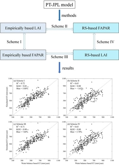
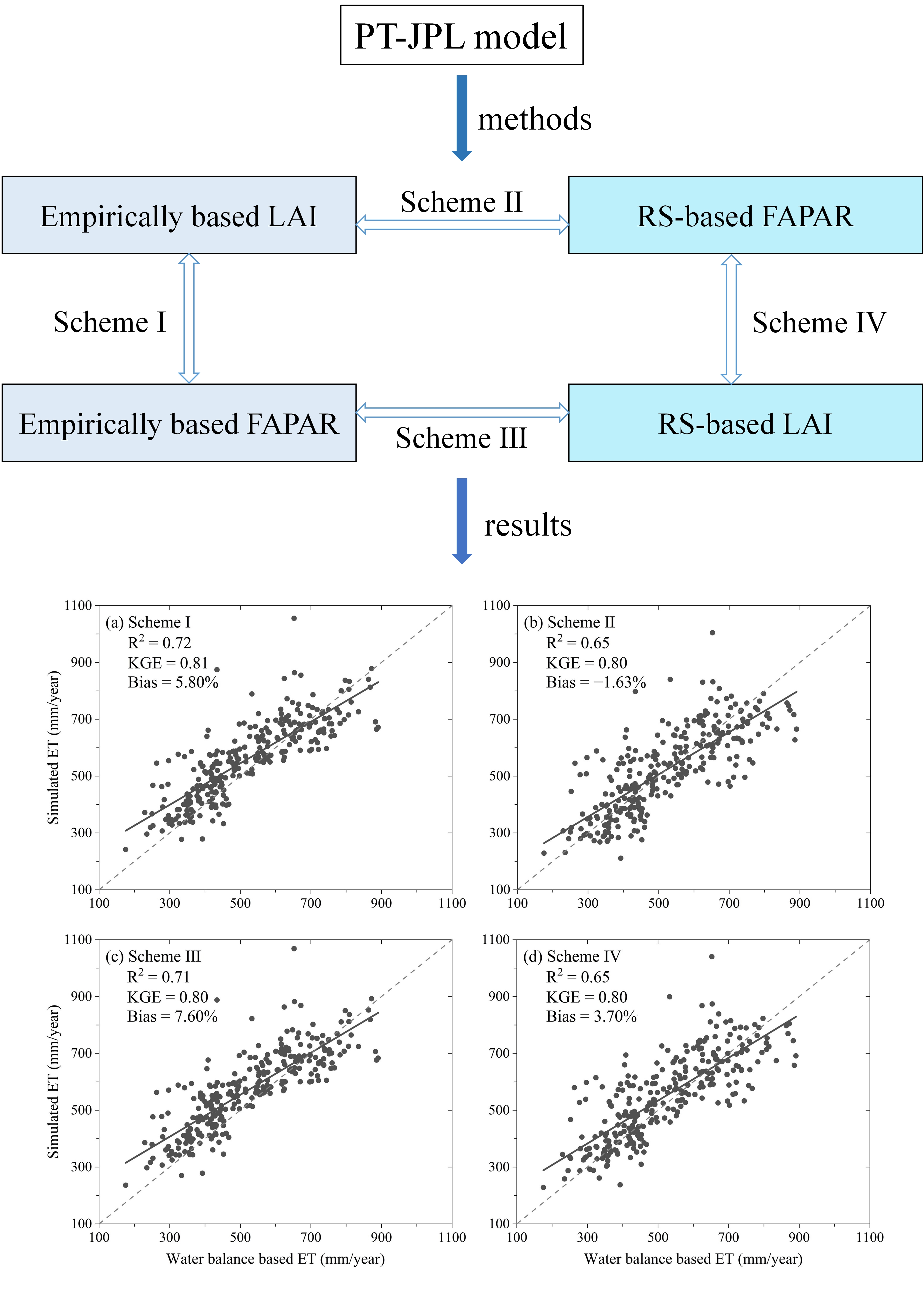
2.2. The Setting of Vegetation Input Schemes for the PT-JPL Model

The PT-JPL model contains three vegetation variables: LAI, FAPAR, and FIPAR. LAI and FAPAR can be obtained from multiple RS data sources [43,44,45,46,47], while global RS FIPAR product is not available. Here we combine LAI and FAPAR estimates from empirical methods and RS products into four vegetation input schemes for the PT-JPL model (Figure 1):

(I)

empirically based LAI and FAPAR (the baseline scheme),

(II)

empirically based LAI and RS-based FAPAR,

(III)

RS-based LAI and empirically based FAPAR,

(IV)

RS-based LAI and FAPAR.

The specific empirical equations used for LAI and FAPAR estimation can be found in Table 1. RS-based LAI and FAPAR refer to the GLASS LAI and FAPAR products [44]. The GLASS LAI product is generated from general regression neural networks, and it showed high accuracy during comparison with similar products and validation with in situ observations [48]. The GLASS FAPAR product is derived from the GLASS LAI product through a series of algorithms [45]. The two products have a spatial resolution of 0.05° and a time span from 1981 to 2018. The NDVI dataset is obtained from the Global Inventory Monitoring and Modeling System (GIMMS) project [49]. This dataset is generated from multiple satellite sensors and considers multiple factors affecting data quality, such as calibration loss, orbital drift, and volcanic eruptions [50].

2.3. The Forcing Data and Evaluation Data for the PT-JPL Model

The forcing data of the PT-JPL model includes meteorological data and albedo data in addition to vegetation input data. Meteorological data includes daily temperature, relative humidity, wind speed, and sunshine duration. We use a professional meteorological interpolation software, namely the Anusplin [51], to interpolate the gauge-based data to gridded data. The Anusplin’s algorithm can consider the effect of terrain on interpolated variables. The albedo and sunshine duration data are used to calculate the R_n, following the method of Allen et al. [19]. We validate R_n estimates with flux site observations. The results indicate that there is a good agreement between our estimated R_n and observed R_n (see Figure S1). The resolution of original NDVI data is 1/12 degree, and the data is resampled to 0.05° × 0.05° with the nearest neighbor resampling approach [52]. The 8-day or half-month RS vegetation data are linearly interpolated to the daily data to match the time step at which the model runs. Natural runoff data from 1981 to 2000 are provided by the Hydrological Bureau of the Ministry of Water Resources in China. More information on the forcing and validation data of the PT-JPL model can be found in

Table 2. Details of model forcing data and evaluation data.

Data Type	Name	Sources
Meteorological forcing data	Precipitation	CMA (http://data.cma.cn/) (accessed on 15 May 2022)
	Relative humidity	Idem
	Temperature	Idem
	Wind speed	Idem
	Sunshine duration	Idem
Land surface data	NDVI [1/12 degree]	https://ecocast.arc.nasa.gov/data/pub/gimms/3g.v1 (accessed on 15 May 2022)
	Albedo [0.05 degree]	http://www.glass.umd.edu/Download.htm (accessed on 21 May 2022)
	LAI [0.05 degree]	Idem
	FAPAR [0.05 degree]	Idem
Evaluation data	River discharge	Hydrological Bureau of the Ministry of Water Resources in China
	ET flux	ChinaFLUX (http://www.chinaflux.org/) (accessed on 30 March 2022), FLUXNET2015 (https://fluxnet.org/data/fluxnet2015-dataset/) (accessed on 26 January 2022), and Science Data Bank (http://www.sciencedb.cn/dataSet/handle/939) (accessed on 18 May 2022)
	GLEAM v3.5 [0.25 degree]	https://www.gleam.eu/ (accessed on 16 February 2022)

.

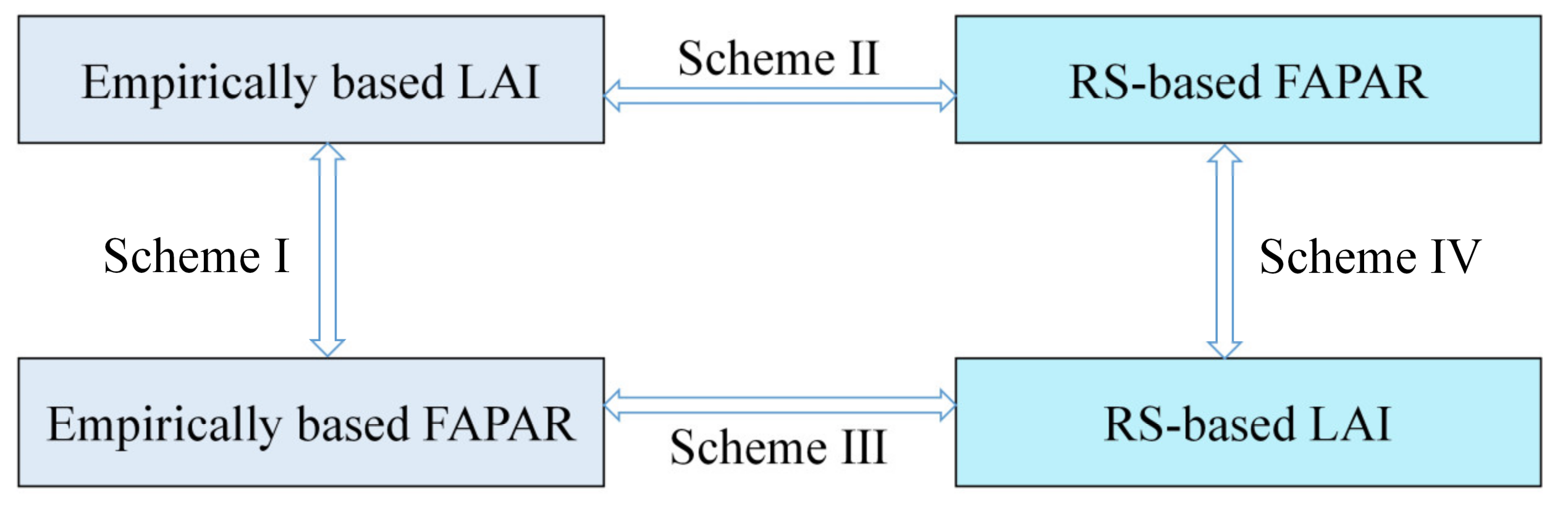
The performance of the PT-JPL model under four vegetation input schemes is evaluated at the site and basin scales. At the site scale, the EC-based ET measurements from 10 ChinaFlux sites are used as the benchmark data to evaluate the model performance (see

Table 3. The information on the ten flux sites. MAP: mean annual precipitation; MAT: mean annual temperature.

Station	Ecosystem Type	Elevation (m)	MAP (mm/Year)	MAT (°C)	Time Range
CBS	Mixed forests	738	713	3.6	2003–2010
QYZ	Evergreen Needleleaf Forests	110	1542	17.9	2003–2010
DHS	Evergreen Broadleaf Forests	300	1956	20.9	2003–2010
NMG	Grasslands	1200	338	0.9	2007–2010
DL	Grasslands	1350	319	2.0	2006–2008
DX	Grasslands	4333	450	1.3	2004–2010
CL	Grasslands	171	315	7.5	2007–2010
HB	Shrublands	3190	535	−1.2	2003–2010
YC	Croplands	28	582	13.1	2003–2010
LC	Croplands	50	490	12.9	2007–2013

). These flux sites cover different types of ecosystems in China, including three forest sites, four grassland sites, one shrubland site, and two cropland sites (Figure 2 and Table 3). The main crop types at the two cropland sites are winter wheat and summer maize. The observation data from rainy days (daily precipitation greater than 0.5 mm) are excluded from model evaluation given the potentially large observation errors on rainy days. At the basin scale, the water balance-based ET estimates are used to validate the PT-JPL model’s performance. The water balance method assumes that the total storage change (ΔS) can be ignored on the mean annual scale. Then, mean annual ET can be estimated as the difference between precipitation (P) and runoff (R): ET = P-R. This method has been widely used for the basin-scale ET evaluation [53,54]. A total of 286 basins are used here (Figure 2), and these basins cover diverse climatic and landscape conditions, with the aridity index ranging from 0.47 to 2.73 [55]. The basin-scale model evaluation is only performed for the period 1982–2000 because runoff data outside this period are not available. In addition, the Global Evaporation Amsterdam Model (GLEAM) ET product (version 3.5) [56,57] is used to evaluate the reliability of ET component partitioning for the PT-JPL model.

2.4. Model Performance Assessment

Three model performance indicators are used: coefficient of determination (R²), percent relative bias (Bias, %), and Kling-Gupta efficiency (KGE) [58]. The value of R² ranges from 0 to 1, and R² = 1 is the optimal value. Bias measures the degree to which simulations are overestimated (positive value) or underestimated (negative value) relative to observations, and it ranges from −∞ to +∞, with an optimal value of zero. KGE is a comprehensive indicator to measure the consistency between simulations and observations. It integrates three independent indicators (bias, variance, and correlation) into one function [59]. The value of KGE is in the range between −∞ and 1.0, with an optimal value of 1.0.

3. Results

3.1. Comparison of Vegetation Variables Estimated by Empirical and Remote Sensing Methods

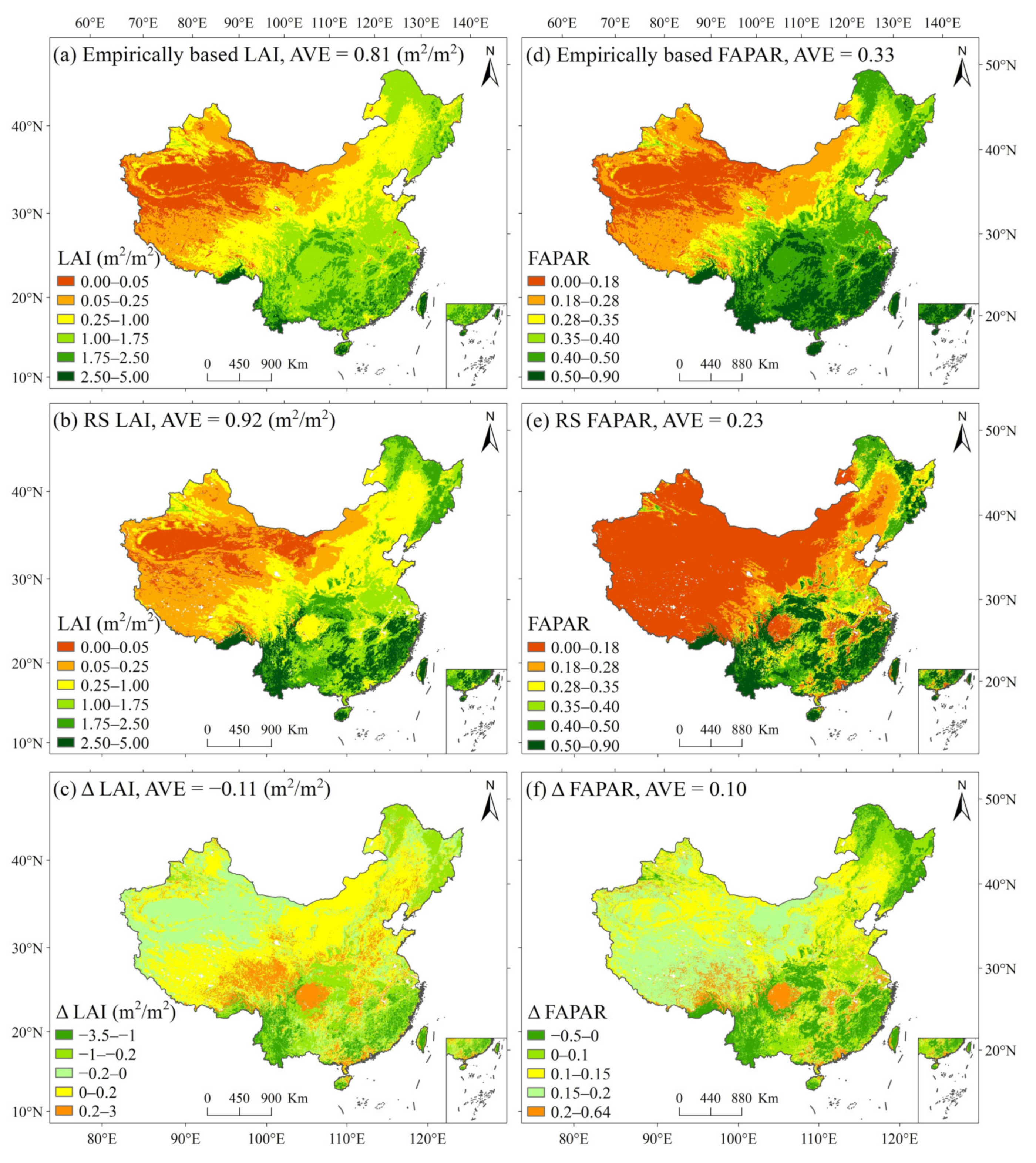
We compare LAI and FAPAR estimated by empirical methods and RS (GLASS) products. Figure 3 shows the spatial patterns of mean annual LAI (FAPAR) estimates from the two methods and their difference across China. The empirically based LAI shows a similar spatial pattern to RS LAI, with a decreasing trend from southeast to northwest China (Figure 3a,b). However, the two methods have significant differences in LAI estimates, particularly in well-vegetated areas (Figure 3c). On a national scale, mean annual LAI estimates from the empirical method and RS product are 0.81 and 0.92 m²/m², respectively. The empirically based LAI has lower values than RS LAI in most areas. The FAPAR estimated by the two methods shows a similar spatial pattern to the LAI (Figure 3d,e), and empirically based FAPAR in most areas is higher than RS FAPAR (Figure 3f).

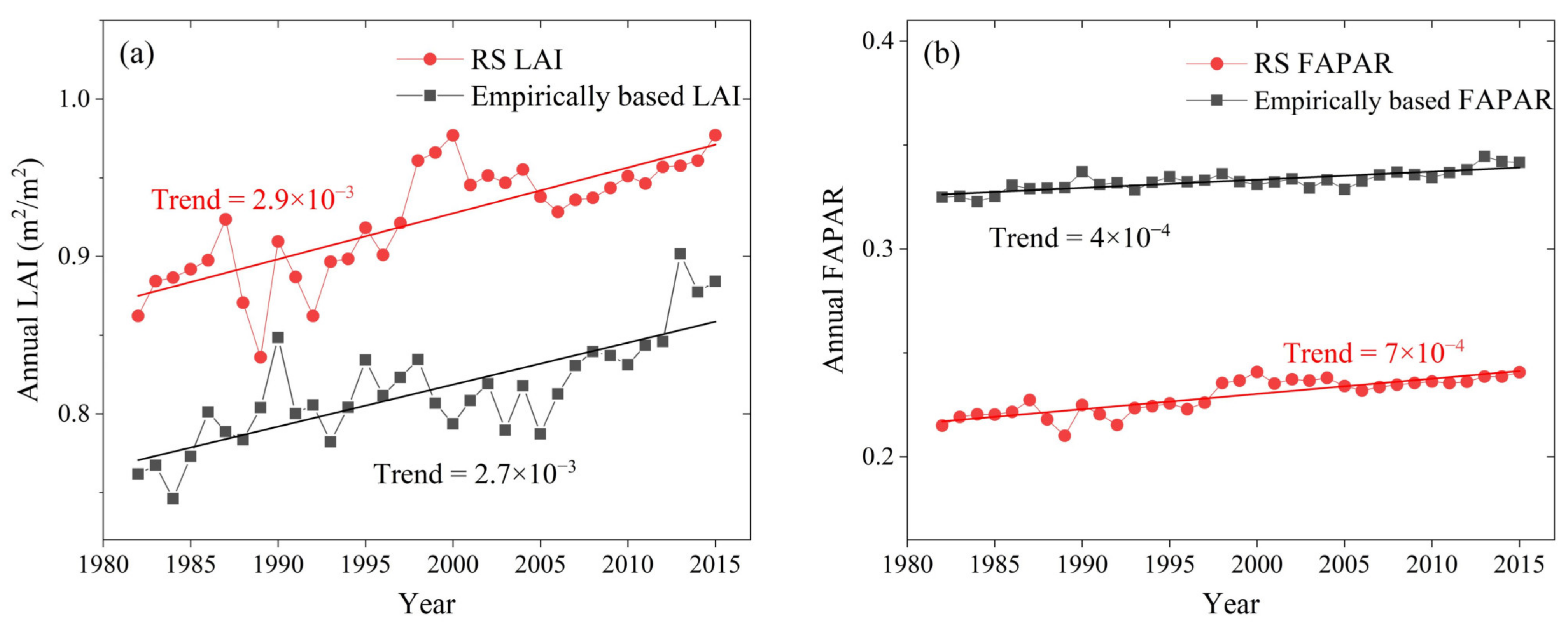
We also compare the interannual changes of national-scale LAI (Figure 4a) and FAPAR (Figure 4b) estimated by the two methods from 1982 to 2015. The empirically based LAI is apparently less than RS LAI, but the empirically based FAPAR is always larger than RS FAPAR. The annual trends of the two vegetation variables from RS products ((LAI: 2.9 × 10⁻³, FAPAR: 7 × 10⁻⁴) are larger than those from empirical methods (LAI: 2.7 × 10⁻³, FAPAR: 4 × 10⁻⁴).

3.2. The Difference in ET Estimates under Four Vegetation Input Schemes

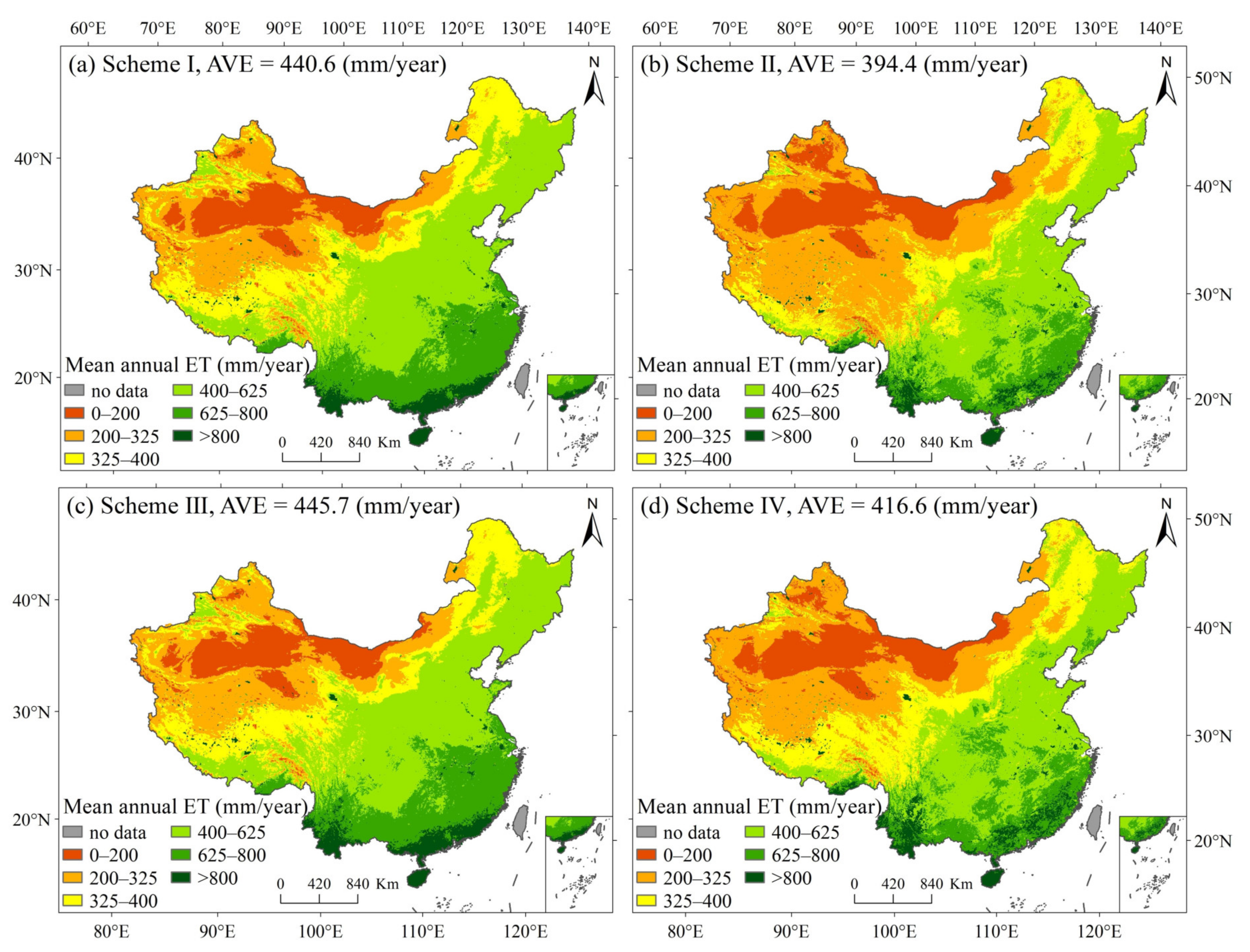
We compare mean annual ET estimates of the PT-JPL model under four vegetation input schemes (Figure 5). Mean annual ET estimates from the four schemes show a consistent spatial pattern: a decreasing trend from southeast to northwest China. However, there are pronounced differences in national average ET estimates under the four schemes. Mean annual ET estimates from schemes I and III are close (440.6 mm/year versus 445.7 mm/year), and their values are significantly larger than those obtained from schemes II (394.4 mm/year) and IV (416.6 mm/year). Spatial differences in mean annual ET estimates under the four schemes are mainly reflected in areas with higher ET values, such as southeast China.

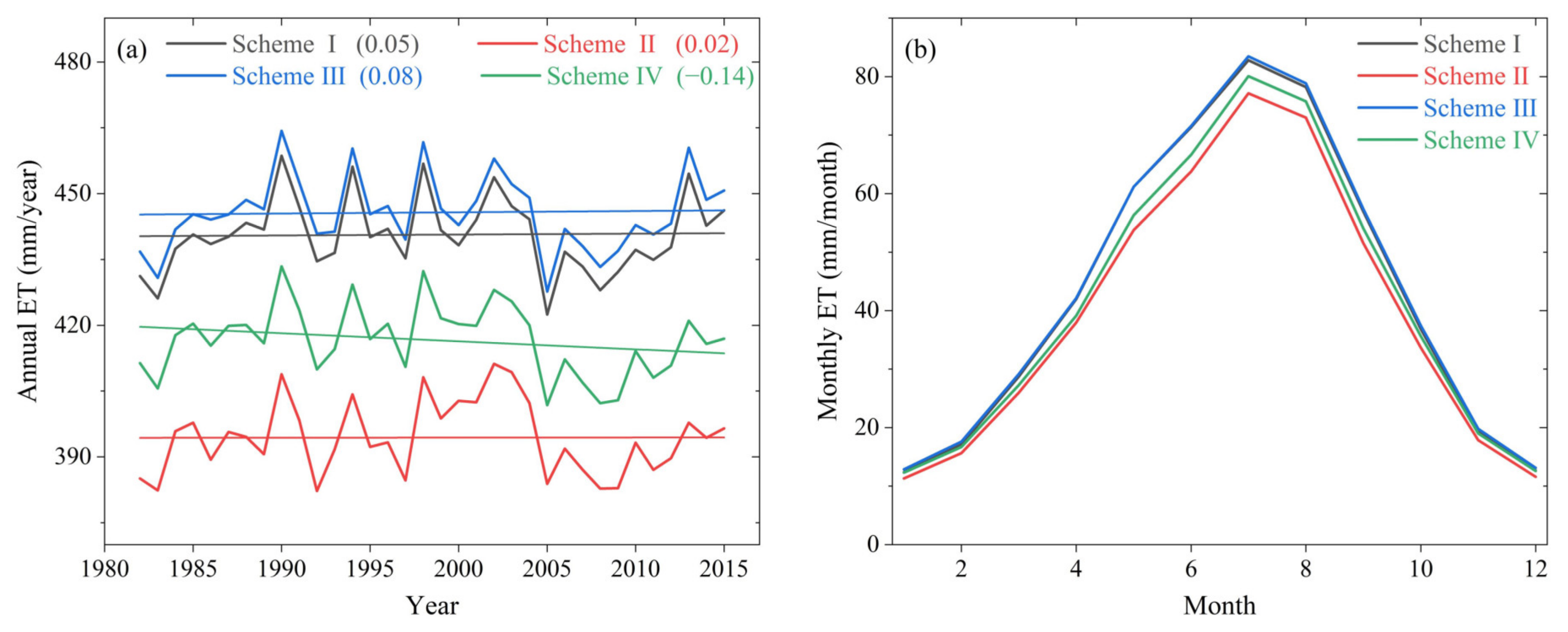
We also compare the interannual variability and seasonal cycle of national average ET estimates under the four schemes from 1982 to 2015 (Figure 6). National-scale annual ET estimates show similar interannual variability but different trends under the four schemes. The trends in annual ET under the four schemes (from I to IV) are 0.05, 0.02, 0.08, and −0.14 mm/year, respectively. The four schemes produce a reverse V-shape intra-annual variation of ET, and the highest values occur in July (Figure 6b). Mean monthly ET estimates from schemes I and III are close to each other, and their values are apparently higher than those from schemes II and IV.

3.3. ET Assessment at the Site and Basin Scales

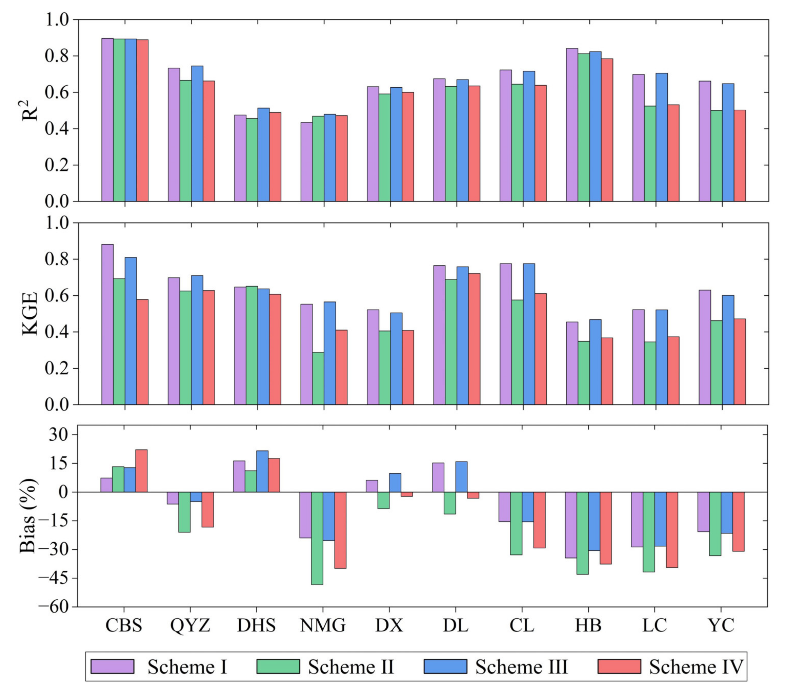
We use the EC-based ET observations from ten flux sites to evaluate the performance of the PT-JPL model under four vegetation input schemes (Figure 7). In terms of the KGE score, scheme I performs best and slightly outperforms scheme III, followed by schemes II and IV. The average KGE values of the ten flux sites under the four schemes are 0.65, 0.51, 0.64, and 0.52, respectively. In terms of ecosystem types, scheme I still outperforms other schemes. For example, the average KGE scores of the forest sites (CBS, QYZ, and DHS) under the four schemes are 0.74, 0.66, 0.72, and 0.60, respectively.

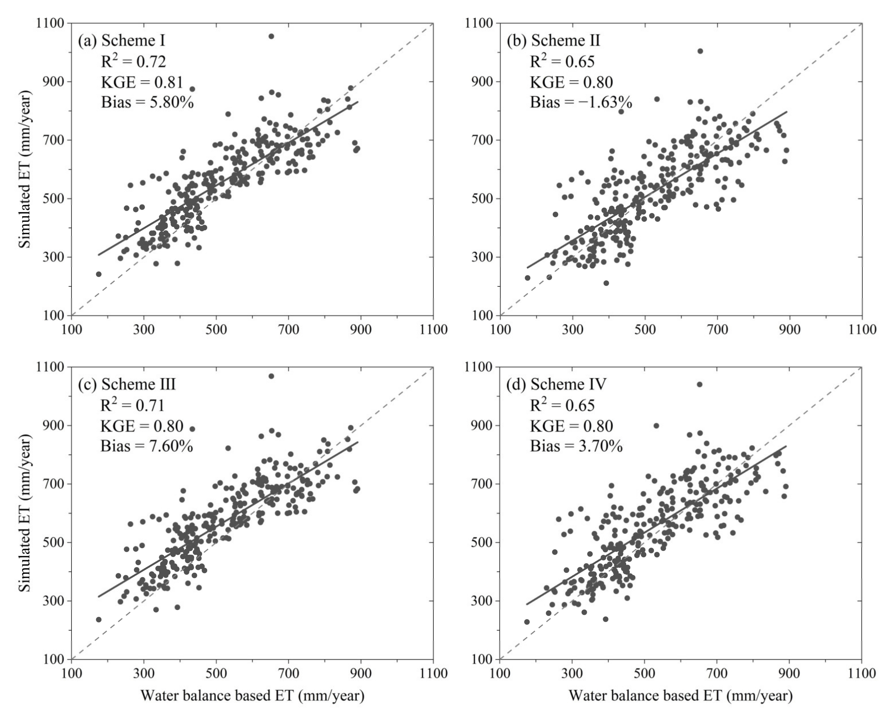
We also evaluate mean annual ET estimates under the four schemes using the water balance-based ET estimates (Figure 8). As shown in Figure 8, scheme I is generally superior to other schemes, which performs best in terms of R² and KGE. The R² values obtained by the four schemes (from I to IV) are 0.72, 0.65, 0.71, and 0.65, respectively. The KGE values under the four schemes are 0.81, 0.80, 0.80, and 0.80, respectively. In addition, scheme III is slightly inferior to scheme I, but it generally outperforms the other two schemes.

4. Discussion

4.1. Why Does Introducing More RS Vegetation Variables beyond NDVI Degrade the Performance of the PT-JPL Model?

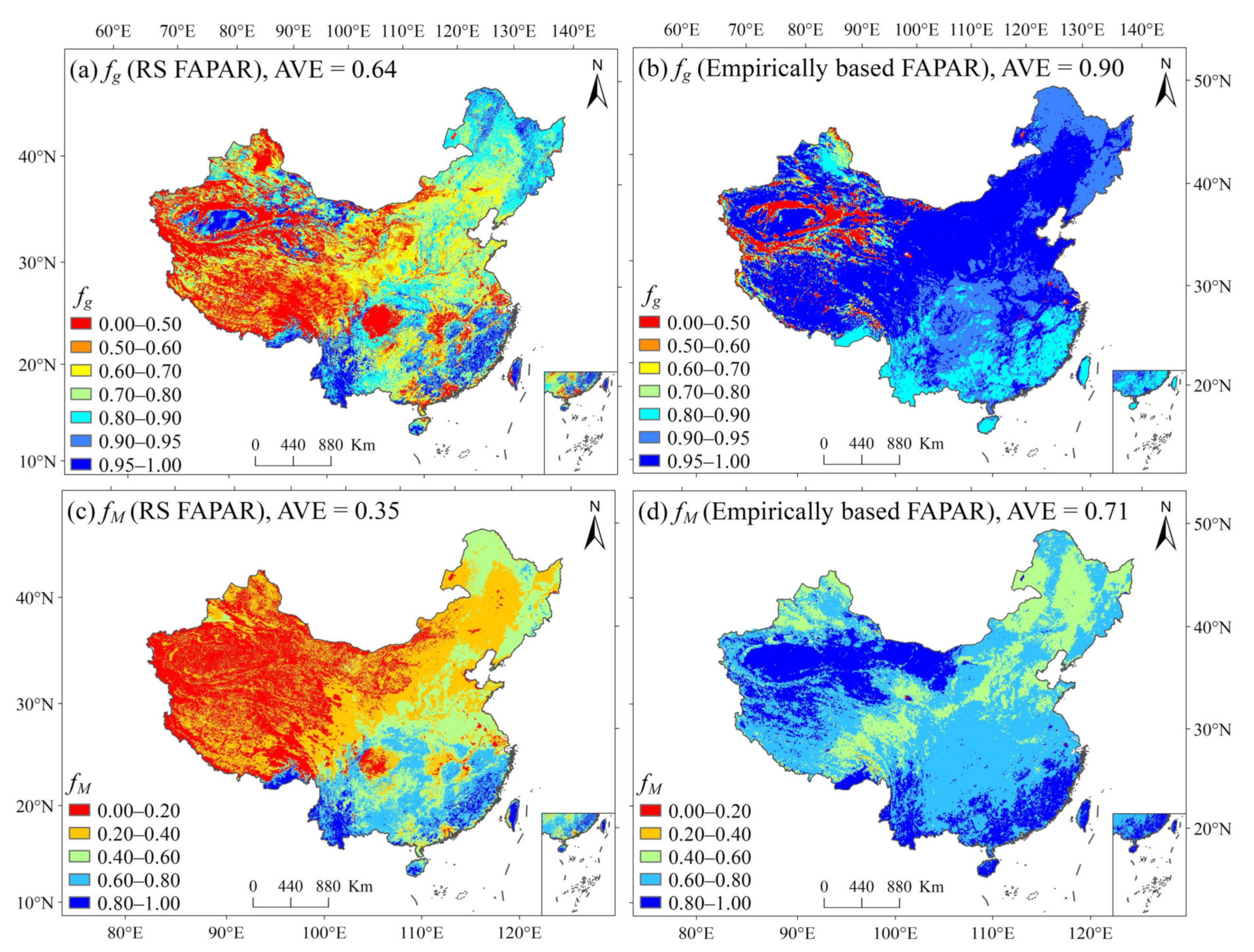
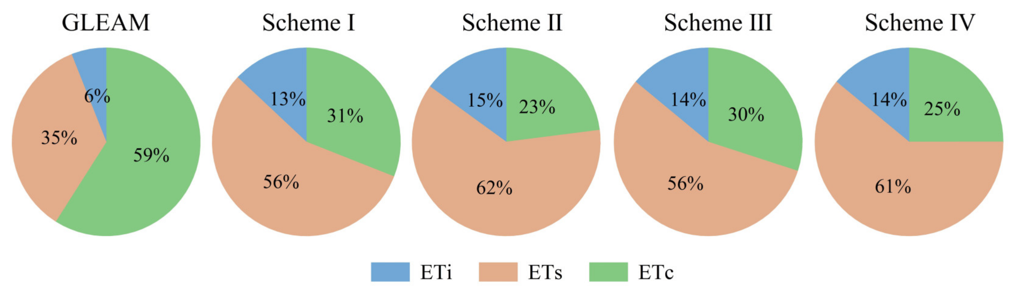
Some RS ET models require multiple vegetation variables as inputs to allocate the energy and construct environmental constraints for ET [2,26,30,60,61]. There are usually two strategies to obtain these vegetation variables. The first strategy is to use the existing RS data as much as possible [2,62,63]. The second strategy is to use a single RS vegetation variable (e.g., NDVI) in combination with empirical equation(s) to estimate other vegetation variables (e.g., LAI and FAPAR). Both strategies have their advantages and shortcomings. The first strategy can make full use of multi-source RS vegetation information, but the uncertainties of RS vegetation variables from different sources may also be propagated into ET simulations [35]. The second strategy simplifies the model’s vegetation inputs but may introduce the uncertainty of empirical equation(s) into ET simulations [64]. This study evaluated the performance of the PT-JPL model under the above two strategies and their combinations. We first compared the differences in two vegetation inputs (LAI and FAPAR) estimated by empirical methods and RS products. The results indicated that there are considerable differences in the LAI and FAPAR estimated by the two methods (Figure 3 and Figure 4). Considering that the RS LAI and FAPAR products are generated based on complex algorithms and have been extensively verified globally [48,65], we have reason to believe that the two vegetation variables estimated by empirical methods have larger uncertainties than RS products. Figure 9 confirms our hypotheses that the RS-derived green canopy fraction (f_g) and plant moisture constraint (f_M) (see Table 1) are more reasonable on spatial patterns than those estimated by empirical equations. The RS-derived f_g and f_M show similar spatial patterns to LAI and aridity index (Figure 9a,c), respectively, which match the physical meaning represented by the two state variables. In contrast, the empirically based f_g and f_M are much higher than those derived by RS products, and their spatial patterns are unreasonable in terms of the physical meaning they represent. However, why do better f_g and f_M estimates not yield better ET simulations? To answer this question, we further examined the proportion of ET components (ET_i, ET_s, and ET_c) across China under the four vegetation input schemes. An extensively validated global ET product, namely the Global Land Evaporation Amsterdam Model (GLEAM v3.5) [56,57], was used as benchmark data to evaluate the reliability of ET component partitioning for the PT-JPL model. Under the four vegetation input schemes, the PT-JPL model yields a much larger contribution from ET_i (13–15%) than the GLEAM (6%) product in China (Figure 10), and the contribution of ET_i to ET even exceeds 40% in parts of southern China (see Figure S2). Some studies have also reported the overestimation of ET_i by the PT-JPL model [66,67]. The reason for the overestimation of ET_i in the PT-JPL model is most likely the unreasonable parameterization of relative surface wetness (f_wet, it is also called the faction of wet canopy). The PT-JPL model uses relative humidity (RH) to parameterize f_wet (f_wet = RH⁴) if RH > 70%. This implies that ET_i occurs as long as RH > 70%, even in the absence of precipitation. This assumption is problematic since RH and precipitation are often decoupled, especially in humid regions of China, where there are many days during a year when RH > 70% but no precipitation occurs.

In addition to the overestimation of ET_i, the proportion of transpiration (ET_c) to ET from the PT-JPL model is likely to be underestimated (see Figure 10). Three potential reasons contribute to the low proportion of ET_c to ET across China. First, the energy allocated to the canopy layer was underestimated due to the underestimation of LAI (see Figure 4a). The LAI defined in the original PT-JPL model is the total LAI, while GLASS LAI is essentially the green LAI. In theory, the GLASS LAI should be less than or equal to total LAI if a reasonable LAI parameterization is used. However, the NDVI-derived LAI is significantly smaller than the RS LAI (see Figure 4a). Second, ET_c may be over-constrained in the PT-JPL model: three biophysical constraints (f_g, f_T, and f_M) are used in the model. A low value for any of these constraints would make ET_c much smaller than its potential value (the value under unstressed conditions). By contrast, the GLEAM uses the same method of potential evaporation as the PT-JPL but only uses a soil water constraint to reduce potential evaporation to actual evaporation [56,57]. Third, the proportion of ET_s to ET may be overestimated in the PT-JPL model to offset the underestimation of ET_c, thereby ensuring the rationality of ET simulations. The overestimation of ET_s is achieved by the underestimation of LAI and the overestimation of soil moisture constraint (f_SM). The model calculates the f_SM with daily relative humidity and VPD. This constraint may well reflect the soil moisture status in humid areas but not in arid areas [68]. For example, the desert and Gobi areas of northwest China have extremely dry climates, where the mean annual aridity index exceeds 5.0 (see Figure S3). The real f_SM in these areas should be close to zero, but f_SM estimates in these areas range from 0.3 to 0.6. Overall, the PT-JPL model provides an efficient tool to simulate ET, but the rationality of ET partitioning needs to be revisited. The unrealistic ET portioning is largely attributable to inadequate model constraint schemes, that is, “getting the right results for the wrong reasons.” This explains why introducing more remote sensing variables other than NDVI degrades the model’s performance to varying degrees.

From the perspective of the model application, it is redundant to introduce more RS vegetation variables beyond NDVI, if we only pursue the rationality of ET simulations. However, model users sometimes need to divide ET components reasonably. In this case, it is necessary to re-parameterize the biophysical constraints of the PT-JPL model to achieve a reasonable ET partitioning. Specific model improvement suggestions are summarized as follows: (i) increasing the exponent of the f_wet function (f_wet = RH⁴) to reduce the fraction of ET_i to ET, (ii) introducing RS LAI and FAPAR data, and (iii) re-parameterizing the biophysical constraints based on multi-source ET observations.

4.2. The Model Sensitivity to Vegetation Variables

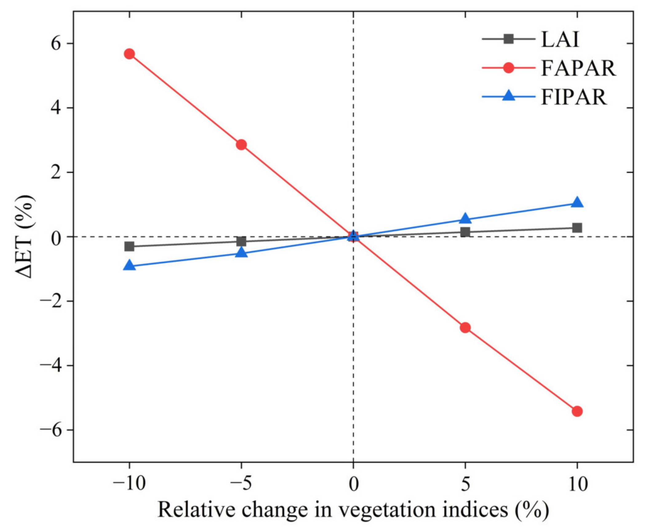
The differences in ET simulations between different vegetation input schemes essentially reflect the model sensitivity to vegetation input variables. For example, the LAI estimates from schemes I and III differ greatly (Figure 4a), but little difference in ET estimates was found between the two schemes. This means that the model is not sensitive to the input of LAI. To fully demonstrate the model sensitivity to vegetation input variables (LAI, FAPAR, and FIPAR), we exerted four perturbations (−10%, −5%, 5%, 10%) to each vegetation variable one by one and then calculated the relative difference in ET simulations (ΔET, %) from baseline simulations (the results of the scheme I). The larger the ΔET, the more sensitive the model is to the change in vegetation variable. The results show that the PT-JPL model is most sensitive to the change in FAPAR, followed by FIPAR and LAI (Figure 11). This result explains why schemes I and III behave similarly, while considerable differences exist between the scheme I and schemes II and IV.

4.3. Potential Uncertainty Sources

Many factors can cause uncertainty in the evaluation results. First, the EC-based ET measurements have two inherent deficiencies: the non-closure of energy balance components and the scale mismatch during the “site-to-pixel” model evaluation [4]. The issue of energy balance non-closure has been observed on almost all flux stations globally [69,70,71]. The non-closure degree of surface energy components in some European sites is generally between 10–30%, as reported by Mauder et al. [72]. Numerous factors affect the closure degree of the energy balance components, including the sampling errors, instrument bias, neglected energy sinks, and horizontal and/or vertical advection of heat and water vapor [69]. In addition, the spatial representation of an EC flux tower is about several hundred square meters, depending on the measured height above the canopy layer and wind speeds [9]. However, the grid area of the model calculation is about 18–29 km² (depending on the altitude). The scale mismatch also has the capacity to skew evaluation results, given the nature of considerable spatial heterogeneity in ET [4]. The uncertainty in the water balance-based ET estimates may also affect the evaluation results. The water balance method assumes that the changes in water storage (S) can be ignored on the mean annual timescale, and then the basin-average ET is estimated as the difference between precipitation and runoff. However, the assumption of S = 0 may not hold, especially in small basins [53,73]. Small basins often have frequent water exchange with neighboring basins, and ignoring this part of the water may result in a large bias in ET estimation from the water balance method [74].

The uncertainty of the forcing data is an important error source for ET simulations [75]. In this study, the meteorological variables from 824 meteorological stations were interpolated into gridded data to drive the PT-JPL model. However, the spatial distribution of these stations is sparse and uneven, especially in the western regions (see Figure 2). This may affect the accuracy of the interpolated meteorological data. In addition, R_n is the key input for the PT-JPL model, and its error may greatly affect the output of the PT-JPL model [26,75]. However, R_n is not a routine observation item of meteorological stations in China. Here we use the sunshine duration, RS albedo, and FAO-56 PM method to calculate the daily R_n [19]. R_n is calculated as the difference between incoming and outgoing radiation of both short and long wavelengths. This method itself has some flaws. It uses the air temperature instead of the land surface temperature to calculate the outgoing longwave radiation since the land surface temperature data before 2000 are not available. This may result in bias in R_n estimates [31]. Nevertheless, the validation results at flux sites indicated that the R_n estimates from the FAO-56 PM method are generally reliable.

The PT-JPL model under the four vegetation input schemes systematically underestimates the ET at the two cropland sites (see Figure 7). This may be due to the effect of agricultural irrigation, which can significantly increase the regional ET rate. However, the PT-JPL model does not take into account the effect of irrigation on ET, thus underestimating ET estimates at these sites. Previous studies have also reported the underestimation of ET at these cropland sites [76,77]. In addition, a single RS vegetation data source (i.e., GLASS) was used here, and these data inevitably have varying degrees of uncertainty. Replacing GLASS with other RS data sources may have the effect of skewing the evaluation results.

5. Conclusions

The major purpose of this study is to investigate whether introducing more vegetation variables beyond NDVI into the PT-JPL model can improve the model’s performance. The vegetation variables estimated by empirical methods and RS (GLASS) products were combined into four different vegetation input schemes for the PT-JPL model. We then evaluated the performance of the PT-JPL model under four schemes at the site and basin scales. The main conclusions are as follows.

(1)

Introducing more RS vegetation information beyond NDVI degrades the accuracy of ET simulations for the PT-JPL model to varying degrees.

(2)

A possible reason for this is the misinterpretation of ET components caused by unreasonable parameterization schemes of biophysical constraints.

(3)

It is necessary to re-parameterize the biophysical constraints of the PT-JPL if the rationality of ET component simulations is sought.

This study highlights the importance of vegetation variable inputs from different sources to ET simulations.

References

- Oki, T.; Kanae, S. Global hydrological cycles and world water resources. Science 2006, 313, 1068–1072. [Google Scholar] [CrossRef] [PubMed] [Green Version]
- García, M.; Sandholt, I.; Ceccato, P.; Ridler, M.; Mougin, E.; Kergoat, L.; Morillas, L.; Timouk, F.; Fensholt, R.; Domingo, F. Actual evapotranspiration in drylands derived from in-situ and satellite data: Assessing biophysical constraints. Remote Sens. Environ. 2013, 131, 103–118. [Google Scholar] [CrossRef]
- Mu, Q.; Zhao, M.; Running, S.W. Improvements to a MODIS global terrestrial evapotranspiration algorithm. Remote Sens. Environ. 2011, 115, 1781–1800. [Google Scholar] [CrossRef]
- Bai, P.; Liu, X. Intercomparison and evaluation of three global high-resolution evapotranspiration products across China. J. Hydrol. 2018, 566, 743–755. [Google Scholar] [CrossRef]
- Glenn, E.P.; Huete, A.R.; Nagler, P.L.; Hirschboeck, K.K.; Brown, P. Integrating Remote Sensing and Ground Methods to Estimate Evapotranspiration. Crit. Rev. Plant Sci. 2007, 26, 139–168. [Google Scholar] [CrossRef]
- Guo, M.; Li, J.; Wang, Y.; Long, Q.; Bai, P. Spatiotemporal Variations of Meteorological Droughts and the Assessments of Agricultural Drought Risk in a Typical Agricultural Province of China. Atmosphere 2019, 10, 542. [Google Scholar] [CrossRef] [Green Version]
- Friedl, M. Relationships among remotely sensed data, surface energy balance, and area-averaged fluxes over partially vegetated land surfaces. J. Appl. Meteorol. Climatol. 1996, 35, 2091–2103. [Google Scholar] [CrossRef]
- Mu, Q.; Heinsch, F.A.; Zhao, M.; Running, S.W. Development of a global evapotranspiration algorithm based on MODIS and global meteorology data. Remote Sens. Environ. 2007, 111, 519–536. [Google Scholar] [CrossRef]
- Wang, K.; Dickinson, R.E. A review of global terrestrial evapotranspiration: Observation, modeling, climatology, and climatic variability. Rev. Geophys. 2012, 50, RG2005. [Google Scholar] [CrossRef]
- Zhang, J.; Bai, Y.; Yan, H.; Guo, H.; Yang, S.; Wang, J. Linking observation, modelling and satellite-based estimation of global land evapotranspiration. Big Earth Data 2020, 4, 94–127. [Google Scholar] [CrossRef]
- Zhang, K.; Kimball, J.S.; Running, S.W. A review of remote sensing based actual evapotranspiration estimation. WIREs Water 2016, 3, 834–853. [Google Scholar] [CrossRef]
- Kustas, W.P.; Norman, J.M. Evaluation of soil and vegetation heat flux predictions using a simple two-source model with radiometric temperatures for partial canopy cover. Agric. For. Meteorol. 1999, 94, 13–29. [Google Scholar] [CrossRef]
- Bastiaanssen, W.G.M.; Menenti, M.; Feddes, R.A.; Holtslag, A.A.M. A remote sensing surface energy balance algorithm for land (SEBAL). 1. Formulation. J. Hydrol. 1998, 212–213, 198–212. [Google Scholar] [CrossRef]
- Norman, J.M.; Kustas, W.P.; Humes, K.S. Source approach for estimating soil and vegetation energy fluxes in observations of directional radiometric surface temperature. Agric. For. Meteorol. 1995, 77, 263–293. [Google Scholar] [CrossRef]
- Su, Z. The Surface Energy Balance System (SEBS) for estimation of turbulent heat fluxes. Hydrol. Earth Syst. Sci. 2002, 6, 85–100. [Google Scholar] [CrossRef]
- Cleugh, H.A.; Leuning, R.; Mu, Q.; Running, S.W. Regional evaporation estimates from flux tower and MODIS satellite data. Remote Sens. Environ. 2007, 106, 285–304. [Google Scholar] [CrossRef]
- Penman, H.L. Natural evaporation from open water, bare soil and grass. Proc. R. Soc. London.Ser. A Math. Phys. Eng. Sci. 1948, 193, 120–145. [Google Scholar] [CrossRef] [Green Version]
- Monteith, J.L. Evaporation and environment. In Symposia of the Society for Experimental Biology; Cambridge University Press (CUP): Cambridge, UK, 1965; pp. 205–234. [Google Scholar]
- Allen, R.G.; Pereira, L.S.; Raes, D.; Smith, M. FAO Irrigation and Drainage Paper No. 56; Food and Agriculture Organization of the United Nations: Rome, Italy, 1998. [Google Scholar]
- Stewart, J.B. Modelling surface conductance of pine forest. Agric. For. Meteorol. 1988, 43, 19–35. [Google Scholar] [CrossRef]
- Ball, J.T.; Woodrow, I.E.; Berry, J.A. A model predicting stomatal conductance and its contribution to the control of photosynthesis under different environmental conditions. In Progress in Photosynthesis Research; Springer: Dordrecht, The Netherlands, 1987; pp. 221–224. [Google Scholar]
- Leuning, R.; Zhang, Y.Q.; Rajaud, A.; Cleugh, H.; Tu, K. A simple surface conductance model to estimate regional evaporation using MODIS leaf area index and the Penman-Monteith equation. Water Resour. Res. 2008, 44, W10419. [Google Scholar] [CrossRef]
- Beven, K. A sensitivity analysis of the Penman-Monteith actual evapotranspiration estimates. J. Hydrol. 1979, 44, 169–190. [Google Scholar] [CrossRef]
- Gong, L.; Xu, C.-Y.; Chen, D.; Halldin, S.; Chen, Y.D. Sensitivity of the Penman–Monteith reference evapotranspiration to key climatic variables in the Changjiang (Yangtze River) basin. J. Hydrol. 2006, 329, 620–629. [Google Scholar] [CrossRef]
- Priestley, C.H.B.; Taylor, R.J. On the assessment of surface heat flux and evaporation using large-scale parameters. Mon. Weather Rev. 1972, 100, 81–92. [Google Scholar] [CrossRef]
- Fisher, J.B.; Tu, K.P.; Baldocchi, D.D. Global estimates of the land–atmosphere water flux based on monthly AVHRR and ISLSCP-II data, validated at 16 FLUXNET sites. Remote Sens. Environ. 2008, 112, 901–919. [Google Scholar] [CrossRef]
- McCabe, M.F.; Ershadi, A.; Jimenez, C.; Miralles, D.G.; Michel, D.; Wood, E.F. The GEWEX LandFlux project: Evaluation of model evaporation using tower-based and globally gridded forcing data. Geosci. Model. Dev. 2016, 9, 283–305. [Google Scholar] [CrossRef] [Green Version]
- Ershadi, A.; McCabe, M.F.; Evans, J.P.; Chaney, N.W.; Wood, E.F. Multi-site evaluation of terrestrial evaporation models using FLUXNET data. Agric. For. Meteorol. 2014, 187, 46–61. [Google Scholar] [CrossRef]
- Gomis-Cebolla, J.; Jimenez, J.C.; Sobrino, J.A.; Corbari, C.; Mancini, M. Intercomparison of remote-sensing based evapotranspiration algorithms over amazonian forests. Int. J. Appl. Earth Obs. Geoinf. 2019, 80, 280–294. [Google Scholar] [CrossRef]
- Shao, R.; Zhang, B.; Su, T.; Long, B.; Cheng, L.; Xue, Y.; Yang, W. Estimating the increase in regional evaporative water consumption as a result of vegetation restoration over the loess plateau, china. J. Geophys. Res. Atmos. 2019, 124, 11783–11802. [Google Scholar] [CrossRef]
- Yao, Y.; Liang, S.; Li, X.; Chen, J.; Liu, S.; Jia, K.; Zhang, X.; Xiao, Z.; Fisher, J.B.; Mu, Q.; et al. Improving global terrestrial evapotranspiration estimation using support vector machine by integrating three process-based algorithms. Agric. For. Meteorol. 2017, 242, 55–74. [Google Scholar] [CrossRef]
- Su, Z.; Schmugge, T.; Kustas, W.; Massman, W. An evaluation of two models for estimation of the roughness height for heat transfer between the land surface and the atmosphere. J. Appl. Meteorol. Climatol. 2001, 40, 1933–1951. [Google Scholar] [CrossRef] [Green Version]
- Stisen, S.; Soltani, M.; Mendiguren, G.; Langkilde, H.; Garcia, M.; Koch, J. Spatial patterns in actual evapotranspiration climatologies for europe. Remote Sens. 2021, 13, 2410. [Google Scholar] [CrossRef]
- Jonckheere, I.; Fleck, S.; Nackaerts, K.; Muys, B.; Coppin, P.; Weiss, M.; Baret, F. Review of methods for in situ leaf area index determination: Part I. Theories, sensors and hemispherical photography. Agric. For. Meteorol. 2004, 121, 19–35. [Google Scholar] [CrossRef]
- Chen, H.; Zhu, G.; Zhang, K.; Bi, J.; Jia, X.; Ding, B.; Zhang, Y.; Shang, S.; Zhao, N.; Qin, W. Evaluation of Evapotranspiration Models Using Different LAI and Meteorological Forcing Data from 1982 to 2017. Remote Sens. 2020, 12, 2473. [Google Scholar] [CrossRef]
- Flint, A.L.; Childs, S.W. Use of the Priestley-Taylor evaporation equation for soil water limited conditions in a small forest clearcut. Agric. For. Meteorol. 1991, 56, 247–260. [Google Scholar] [CrossRef]
- Yang, Y.; Roderick, M.L. Radiation, surface temperature and evaporation over wet surfaces. Quart. J. Roy. Meteorol. Soc. 2019, 145, 1118–1129. [Google Scholar] [CrossRef]
- McAneney, K.J.; Itier, B. Operational limits to the Priestley-Taylor formula. Irrig. Sci. 1996, 17, 37–43. [Google Scholar] [CrossRef]
- Impens, I.; Lemeur, R. Extinction of net radiation in different crop canopies. Arch. Für Meteorol. Geophys. Und Bioklimatol. Ser. B 1969, 17, 403–412. [Google Scholar] [CrossRef]
- Ross, J. Chapter 2. Radiative Transfer in Plant Communities. In Vegetation and the Atmosphere; Monteith, J.L., Ed.; Academic Press: London, UK, 1976; Volume 1, pp. 13–55. [Google Scholar]
- Gao, X.; Huete, A.R.; Ni, W.; Miura, T. Optical–biophysical relationships of vegetation spectra without background contamination. Remote Sens. Environ. 2000, 74, 609–620. [Google Scholar] [CrossRef]
- June, T.; Evans, J.R.; Farquhar, G.D. A simple new equation for the reversible temperature dependence of photosynthetic electron transport: A study on soybean leaf. Funct. Plant Biol. 2004, 31, 275–283. [Google Scholar] [CrossRef] [Green Version]
- Claverie, M.; Matthews, J.; Vermote, E.; Justice, C. A 30+ Year AVHRR LAI and FAPAR Climate Data Record: Algorithm Description and Validation. Remote Sens. 2016, 8, 263. [Google Scholar] [CrossRef] [Green Version]
- Xiao, Z.; Liang, S.; Wang, J.; Xiang, Y.; Zhao, X.; Song, J. Long-Time-Series Global Land Surface Satellite Leaf Area Index Product Derived From MODIS and AVHRR Surface Reflectance. IEEE Trans. Geosci. Remote Sens. 2016, 54, 5301–5318. [Google Scholar] [CrossRef]
- Xiao, Z.; Liang, S.; Sun, R.; Wang, J.; Jiang, B. Estimating the fraction of absorbed photosynthetically active radiation from the MODIS data based GLASS leaf area index product. Remote Sens. Environ. 2015, 171, 105–117. [Google Scholar] [CrossRef]
- Zhu, Z.; Bi, J.; Pan, Y.; Ganguly, S.; Anav, A.; Xu, L.; Samanta, A.; Piao, S.; Nemani, R.; Myneni, R. Global Data Sets of Vegetation Leaf Area Index (LAI) 3g and Fraction of Photosynthetically Active Radiation (FPAR)3g Derived from Global Inventory Modeling and Mapping Studies (GIMMS) Normalized Difference Vegetation Index (NDVI3g) for the Period 1981 to 2011. Remote Sens. 2013, 5, 927–948. [Google Scholar] [CrossRef] [Green Version]
- Liu, Y.; Liu, R.; Chen, J.M. Retrospective retrieval of long-term consistent global leaf area index (1981–2011) from combined AVHRR and MODIS data. J. Geophys. Res. Biogeosci. 2012, 117, G04003. [Google Scholar] [CrossRef]
- Xiao, Z.; Liang, S.; Jiang, B. Evaluation of four long time-series global leaf area index products. Agric. For. Meteorol. 2017, 246, 218–230. [Google Scholar] [CrossRef]
- Tucker, C.J.; Pinzon, J.E.; Brown, M.E.; Slayback, D.A.; Pak, E.W.; Mahoney, R.; Vermote, E.F.; El Saleous, N. An extended AVHRR 8-km NDVI dataset compatible with MODIS and SPOT vegetation NDVI data. Int. J. Remote Sens. 2005, 26, 4485–4498. [Google Scholar] [CrossRef]
- Pinzon, J.; Tucker, C. A Non-Stationary 1981–2012 AVHRR NDVI3g Time Series. Remote Sens. 2014, 6, 6929–6960. [Google Scholar] [CrossRef] [Green Version]
- Hutchinson, M.F.; Xu, T. Anusplin version 4.2 user guide. In Centre for Resource Environmental Studies; The Australian National University: Canberra, Australia, 2004; p. 54. [Google Scholar]
- Bai, P.; Liu, X.M.; Zhang, Y.Q.; Liu, C.M. Assessing the impacts of vegetation greenness change on evapotranspiration and water yield in China. Water Resour. Res. 2020, 56, e2019WR027019. [Google Scholar] [CrossRef]
- Zeng, Z.; Piao, S.; Lin, X.; Yin, G.; Peng, S.; Ciais, P.; Myneni, R.B. Global evapotranspiration over the past three decades: Estimation based on the water balance equation combined with empirical models. Environ. Res. Lett. 2012, 7, 014026. [Google Scholar] [CrossRef]
- Senay, G.B.; Leake, S.; Nagler, P.L.; Artan, G.; Dickinson, J.; Cordova, J.T.; Glenn, E.P. Estimating basin scale evapotranspiration (ET) by water balance and remote sensing methods. Hydrol. Process. 2011, 25, 4037–4049. [Google Scholar] [CrossRef]
- Bai, P.; Liu, X.; Zhang, D.; Liu, C. Estimation of the Budyko model parameter for small basins in China. Hydrol. Process. 2020, 34, 125–138. [Google Scholar] [CrossRef]
- Martens, B.; Miralles, D.G.; Lievens, H.; van der Schalie, R.; de Jeu, R.A.M.; Fernández-Prieto, D.; Beck, H.E.; Dorigo, W.A.; Verhoest, N.E.C. GLEAM v3: Satellite-based land evaporation and root-zone soil moisture. Geosci. Model. Dev. 2017, 10, 1903–1925. [Google Scholar] [CrossRef] [Green Version]
- Miralles, D.G.; Holmes, T.R.H.; De Jeu, R.A.M.; Gash, J.H.; Meesters, A.G.C.A.; Dolman, A.J. Global land-surface evaporation estimated from satellite-based observations. Hydrol. Earth Syst. Sci. 2011, 15, 453–469. [Google Scholar] [CrossRef] [Green Version]
- Gupta, H.V.; Kling, H.; Yilmaz, K.K.; Martinez, G.F. Decomposition of the mean squared error and NSE performance criteria: Implications for improving hydrological modelling. J. Hydrol. 2009, 377, 80–91. [Google Scholar] [CrossRef] [Green Version]
- Knoben, W.J.; Freer, J.E.; Woods, R.A. Inherent benchmark or not? Comparing Nash–Sutcliffe and Kling–Gupta efficiency scores. Hydrol. Earth Syst. Sci. 2019, 23, 4323–4331. [Google Scholar] [CrossRef] [Green Version]
- Yao, Y.; Liang, S.; Cheng, J.; Liu, S.; Fisher, J.B.; Zhang, X.; Jia, K.; Zhao, X.; Qin, Q.; Zhao, B.; et al. MODIS-driven estimation of terrestrial latent heat flux in China based on a modified Priestley–Taylor algorithm. Agric. For. Meteorol. 2013, 171–172, 187–202. [Google Scholar] [CrossRef]
- Purdy, A.J.; Fisher, J.B.; Goulden, M.L.; Colliander, A.; Halverson, G.; Tu, K.; Famiglietti, J.S. SMAP soil moisture improves global evapotranspiration. Remote Sens. Environ. 2018, 219, 1–14. [Google Scholar] [CrossRef]
- Moyano, M.; Garcia, M.; Palacios-Orueta, A.; Tornos, L.; Fisher, J.; Fernández, N.; Recuero, L.; Juana, L. Vegetation Water Use Based on a Thermal and Optical Remote Sensing Model in the Mediterranean Region of Doñana. Remote Sens. 2018, 10, 1105. [Google Scholar] [CrossRef] [Green Version]
- Aragon, B.; Houborg, R.; Tu, K.; Fisher, J.B.; McCabe, M. CubeSats enable high spatiotemporal retrievals of crop-water use for precision agriculture. Remote Sens. 2018, 10, 1867. [Google Scholar] [CrossRef] [Green Version]
- Talsma, C.; Good, S.; Miralles, D.; Fisher, J.; Martens, B.; Jimenez, C.; Purdy, A. Sensitivity of Evapotranspiration Components in Remote Sensing-Based Models. Remote Sens. 2018, 10, 1601. [Google Scholar] [CrossRef] [Green Version]
- Xiao, Z.; Liang, S.; Sun, R. Evaluation of Three Long Time Series for Global Fraction of Absorbed Photosynthetically Active Radiation (FAPAR) Products. IEEE Trans. Geosci. Remote Sens. 2018, 56, 5509–5524. [Google Scholar] [CrossRef]
- Talsma, C.J.; Good, S.P.; Jimenez, C.; Martens, B.; Fisher, J.B.; Miralles, D.G.; McCabe, M.F.; Purdy, A.J. Partitioning of evapotranspiration in remote sensing-based models. Agric. For. Meteorol. 2018, 260, 131–143. [Google Scholar] [CrossRef]
- Miralles, D.G.; Jiménez, C.; Jung, M.; Michel, D.; Ershadi, A.; McCabe, M.F.; Hirschi, M.; Martens, B.; Dolman, A.J.; Fisher, J.B.; et al. The WACMOS-ET project—Part 2: Evaluation of global terrestrial evaporation data sets. Hydrol. Earth Syst. Sci. 2016, 20, 823–842. [Google Scholar] [CrossRef] [Green Version]
- Marshall, M.; Tu, K.; Andreo, V. On parameterizing soil evaporation in a direct remote sensing model of ET: PT-JPL. Water Resour. Res. 2020, 56, e2019WR026290. [Google Scholar] [CrossRef]
- Wilson, K.; Goldstein, A.; Falge, E.; Aubinet, M.; Baldocchi, D.; Berbigier, P.; Bernhofer, C.; Ceulemans, R.; Dolman, H.; Field, C. Energy balance closure at FLUXNET sites. Agric. For. Meteorol. 2002, 113, 223–243. [Google Scholar] [CrossRef] [Green Version]
- Mauder, M.; Genzel, S.; Fu, J.; Kiese, R.; Soltani, M.; Steinbrecher, R.; Zeeman, M.; Banerjee, T.; De Roo, F.; Kunstmann, H. Evaluation of energy balance closure adjustment methods by independent evapotranspiration estimates from lysimeters and hydrological simulations. Hydrol. Process. 2018, 32, 39–50. [Google Scholar] [CrossRef]
- Foken, T.; Aubinet, M.; Finnigan, J.J.; Leclerc, M.Y.; Mauder, M.; Paw, U.K.T. Results of a panel discussion about the energy balance closure correction for trace gases. Bull. Am. Meteorol. Soc. 2011, 92, ES13–ES18. [Google Scholar] [CrossRef] [Green Version]
- Mauder, M.; Foken, T.; Cuxart, J. Surface-Energy-Balance Closure over Land: A Review. Bound. Layer Meteorol. 2020, 177, 395–426. [Google Scholar] [CrossRef]
- Han, J.; Yang, Y.; Roderick, M.L.; McVicar, T.R.; Yang, D.; Zhang, S.; Beck, H.E. Assessing the Steady-State Assumption in Water Balance Calculation Across Global Catchments. Water Resour. Res. 2020, 56, e2020WR027392. [Google Scholar] [CrossRef]
- Guo, M.; Li, J.; Wang, Y.; Bai, P.; Wang, J. Distinguishing the Relative Contribution of Environmental Factors to Runoff Change in the Headwaters of the Yangtze River. Water 2019, 11, 1432. [Google Scholar] [CrossRef] [Green Version]
- Badgley, G.; Fisher, J.B.; Jiménez, C.; Tu, K.P.; Vinukollu, R. On uncertainty in global terrestrial evapotranspiration estimates from choice of input forcing datasets. J. Hydrometeorol. 2015, 16, 1449–1455. [Google Scholar] [CrossRef]
- Li, G.; Zhang, F.; Jing, Y.; Liu, Y.; Sun, G. Response of evapotranspiration to changes in land use and land cover and climate in China during 2001–2013. Sci. Total Environ. 2017, 596–597, 256–265. [Google Scholar] [CrossRef]
- Yao, Y.; Liang, S.; Yu, J.; Zhao, S.; Lin, Y.; Jia, K.; Zhang, X.; Cheng, J.; Xie, X.; Sun, L.; et al. Differences in estimating terrestrial water flux from three satellite-based Priestley-Taylor algorithms. Int. J. Appl. Earth Obs. Geoinf. 2017, 56, 1–12. [Google Scholar] [CrossRef]
Figure 1.
The setting of four vegetation input schemes for the PT-JPL model. Empirically based LAI and FAPAR represent LAI and FAPAR estimated by empirical equations. RS-based LAI and FAPAR represent remote sensing retrieved LAI and FAPAR products.
Figure 2.
Locations of the meteorological stations (grey dots), flux stations (red stars) and 286 test basins. The insert shows the spatial pattern of the aridity index, which is defined as the ratio of potential ET (PET) to precipitation (P) at the mean annual scale.
Figure 3.
The spatial pattern of mean annual (1982–2015) LAI estimated by the empirical method (a) and RS (GLASS) product (b), and their differences (ΔLAI) (c). The right column (d–f) is same as the left column, but for the FAPAR. AVE: National average.
Figure 4.
The interannual changes in national-scale LAI (a) and FAPAR (b) estimated by empirical methods and RS (GLASS) products from 1982 to 2015.
Figure 5.
The spatial pattern of mean annual (1982–2015) ET estimates from the PT-JPL model under four vegetation input schemes. AVE: National average.
Figure 6.
The interannual change (a) and seasonal cycle (b) of national average ET estimates under four vegetation input schemes from 1982 to 2015.
Figure 7.
Comparison of the performance of the PT-JPL model at ten flux sites under the four schemes.
Figure 8.
Scatterplots of simulated versus water balance-based mean annual ET at 286 test basins from 1982 to 2000. The dots represent mean annual ET of test basins; the solid line represents the regression line; the dashed line represents the 1:1 line.
Figure 9.
The spatial pattern of mean annual (1982–2015) green canopy fraction (fg) estimated by RS (GLASS) FAPAR (a) and empirically based FAPAR (b). The bottom two panels (c,d) are same as the top two panels, but for the soil moisture constraint (fM) estimation. AVE: National average.
Figure 10.
Pie charts illustrate the national average contribution of each component to total ET for GLEAM and PT-JPL model. ETi: Interception evaporation; ETs: Soil evaporation; ETc: Canopy transpiration.
Figure 11.
The model sensitivity to changes in vegetation variables (LAI, FAPAR, and FIPAR) for the PT-JPL model. The larger the slope of the line, the more sensitive the model is to the change in vegetation variable. ΔET: The relative difference in ET simulations (%).