
Coupled Heterogeneous Tucker Decomposition: A Feature Extraction Method for Multisource Fusion and Domain Adaptation Using Multisource Heterogeneous Remote Sensing Data

Abstract
:
1. Introduction
1.1. Existing Multisource Fusion-Oriented and Domain Adaptation-Oriented Feature Extraction Methods
1.2. Motivation and Contributions
- (1)
- From the perspective of theory, compared with the classical TD and HTD, which can only extract a compressed representation of a single tensor, the proposed C-HTD can be considered a natural extension of the classical TD and HTD that can extract compressed representations of multiple tensors with different dimensions (i.e., heterogeneous tensors) in an associative manner. More importantly, by establishing different coupling constraints, C-HTD can extract complementary information and shared information from the multisource heterogeneous tensors, which dramatically expands the practicability of the TD and HTD techniques;
- (2)
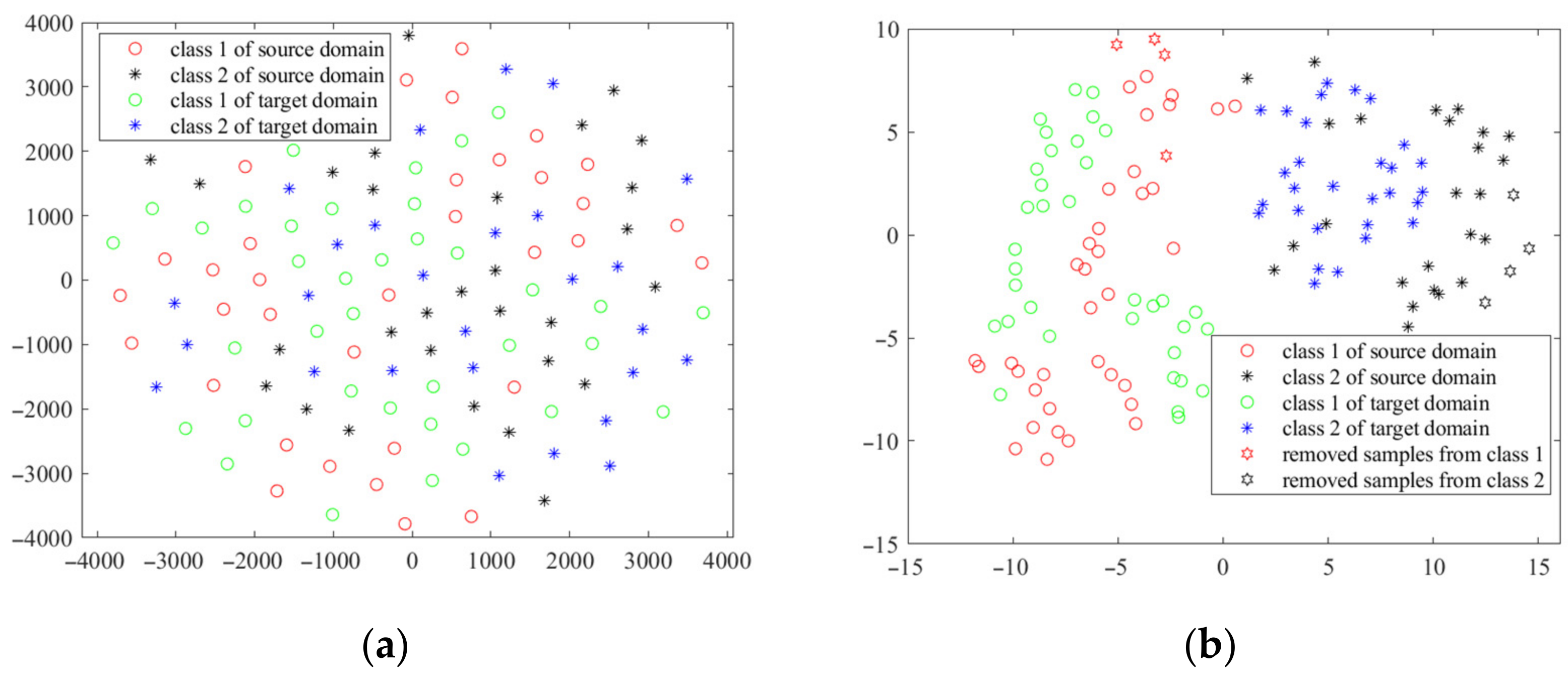
- From the perspective of the application, compared with the existing multisource fusion-oriented and domain adaptation-oriented feature extraction methods that can only deal with vector or homogeneous tensors, the C-HTD is a unified framework that can deal with multisource fusion-oriented and domain adaptation-oriented feature extraction using multisource heterogeneous tensors directly. In addition, the proposed C-HTD can be applied to both supervised and semi-supervised cases by establishing a class-indicator factor matrix along with sample mode. Moreover, unlike the existing domain adaptation methods that are susceptible to outliers, the CCT-HTD can reduce the impact of outliers on domain adaptation results effectively using an adaptive sample-weighing matrix along with sample mode;
- (3)
- To ensure the effective implementation of the proposed C-HTD, the alternative optimization scheme is proposed to solve the optimization problems of CFM-HTD and CCT-HTD to obtain the optimal multisource features and the predicted class labels by sequentially updating the core tensors and a series of factor matrices. Additionally, the detailed theoretical analysis provides the convergence and complexity of C-HTD.
2. Method
2.1. Preliminaries
2.1.1. Notations and Fundamental Tensor Operations
2.1.2. Tucker Decomposition
2.2. Coupled Factor Matrix-Based Heterogeneous Tucker Decomposition
2.2.1. Motivation
2.2.2. Formulation
2.2.3. Optimization
2.3. Coupled Core Tensor-Based Heterogeneous Tucker Decomposition
2.3.1. Motivation
2.3.2. Formulation
3. Results
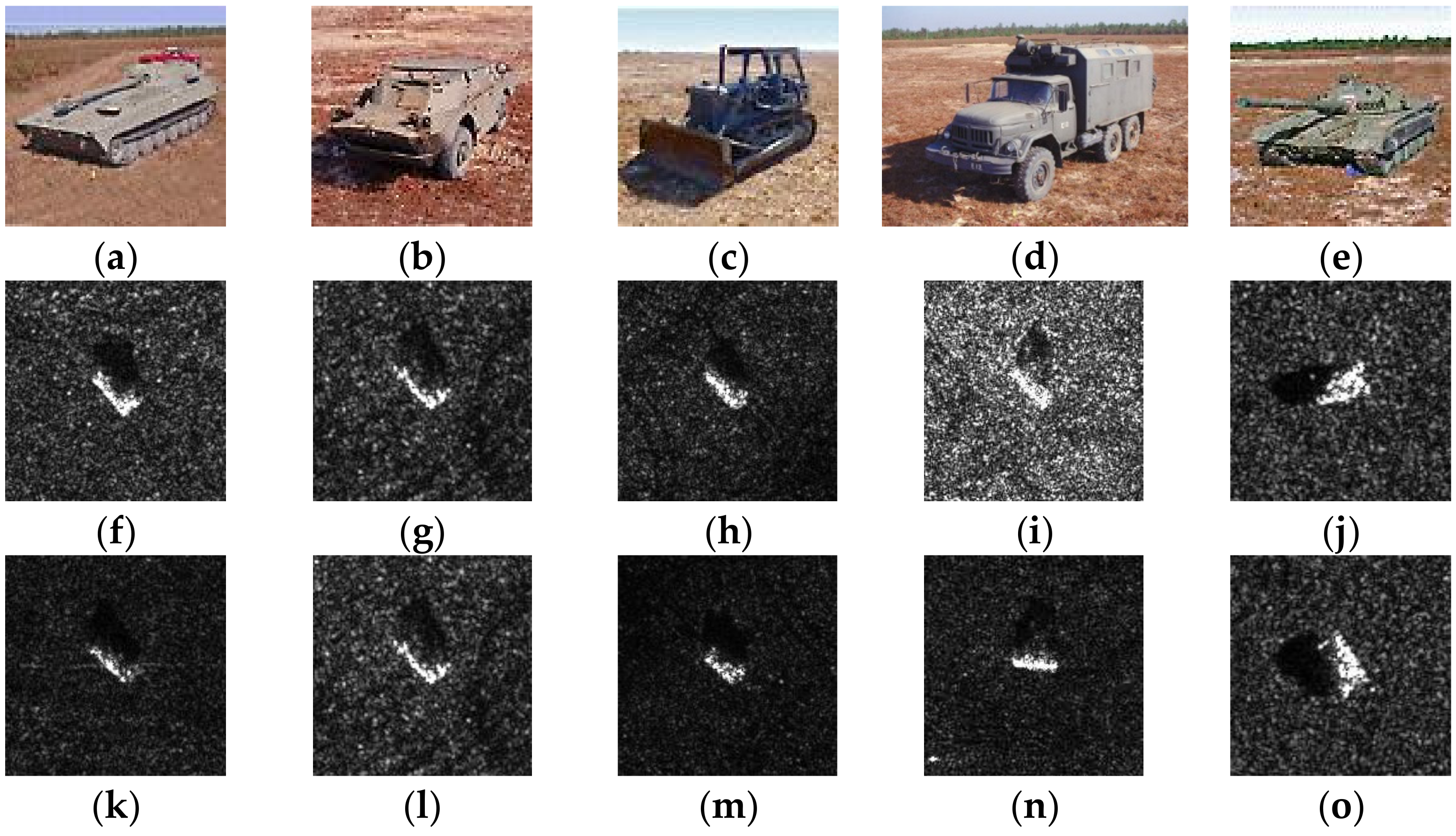
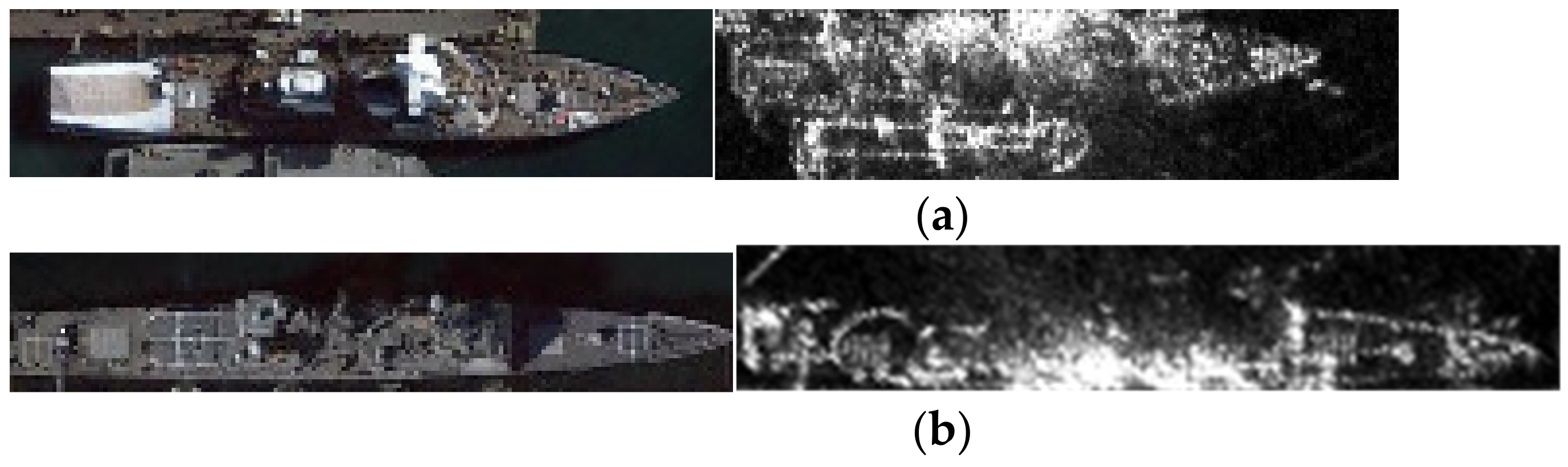
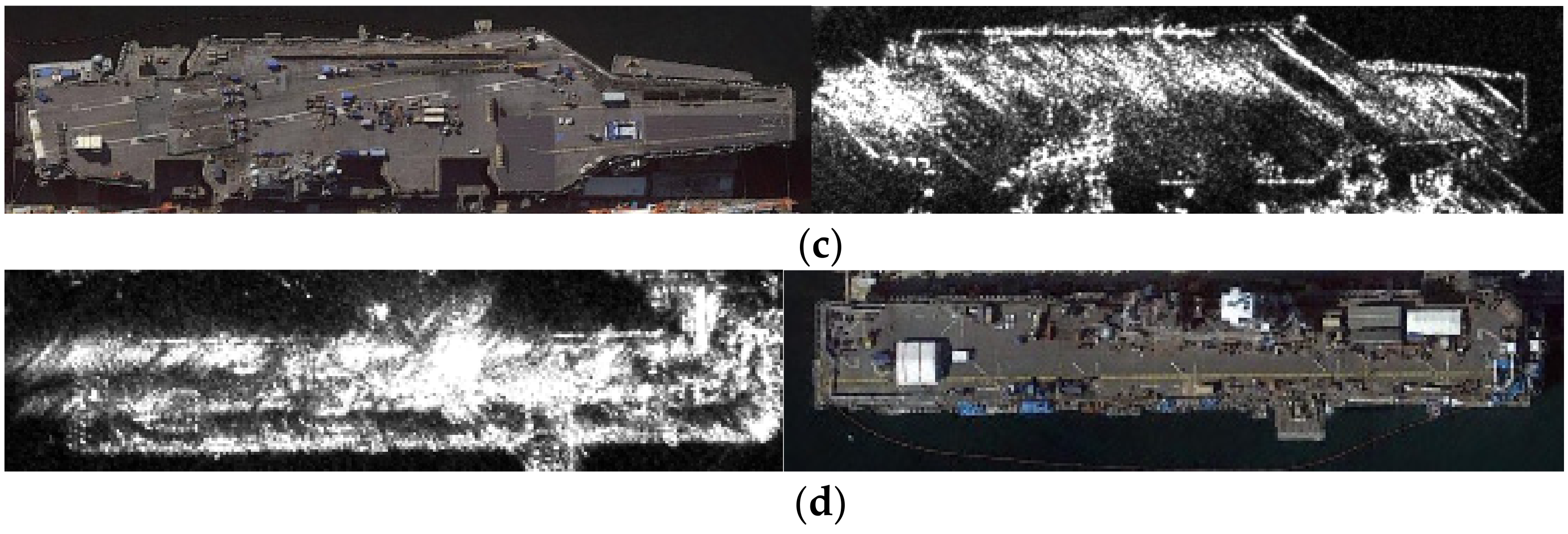
3.1. Datasets
3.2. Construction of Heterogeneous Tensors
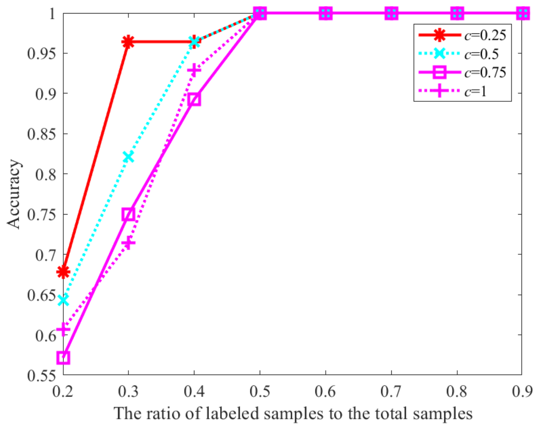
3.3. Analysis of the Impact of Parameter Setting on CFM-HTD
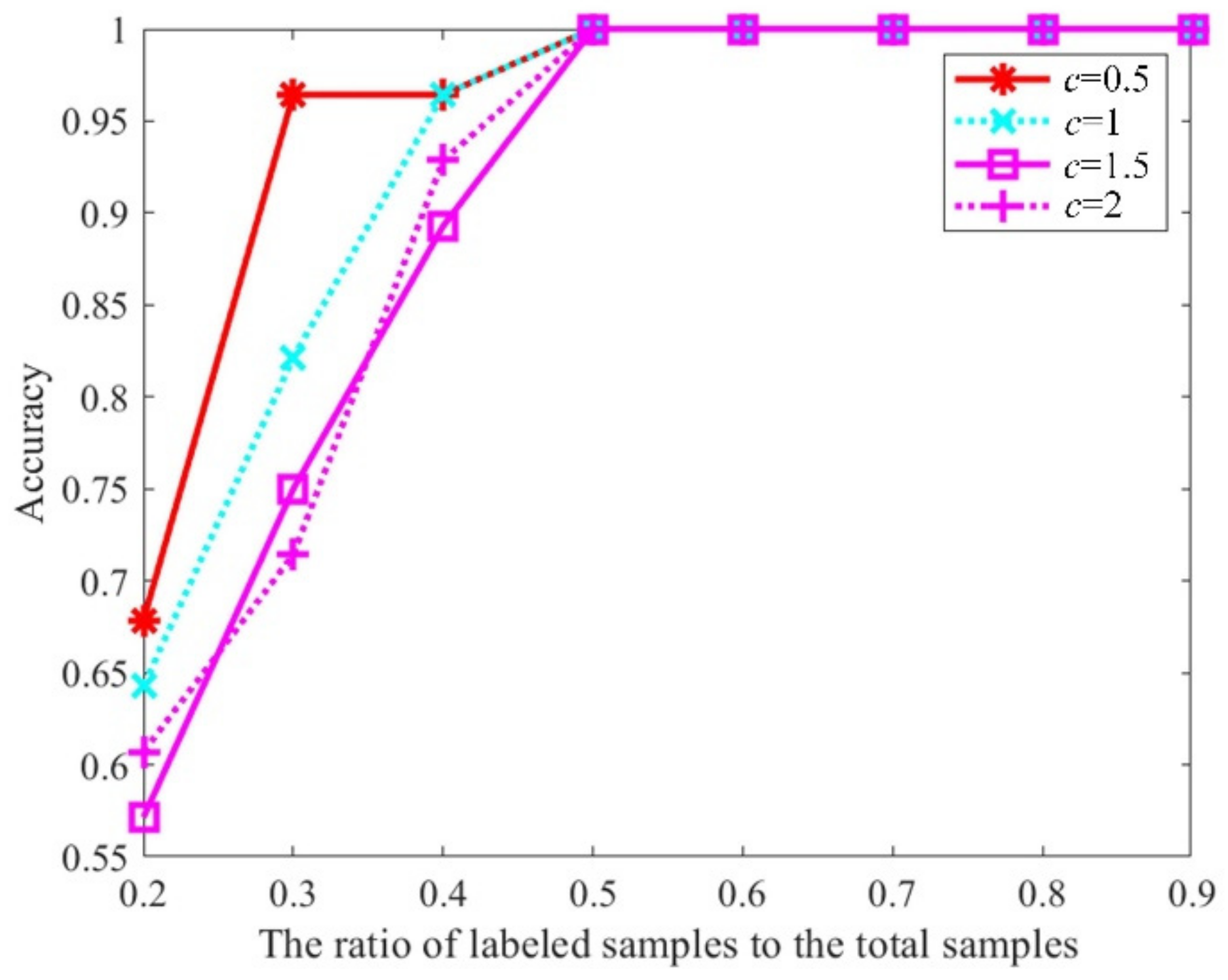
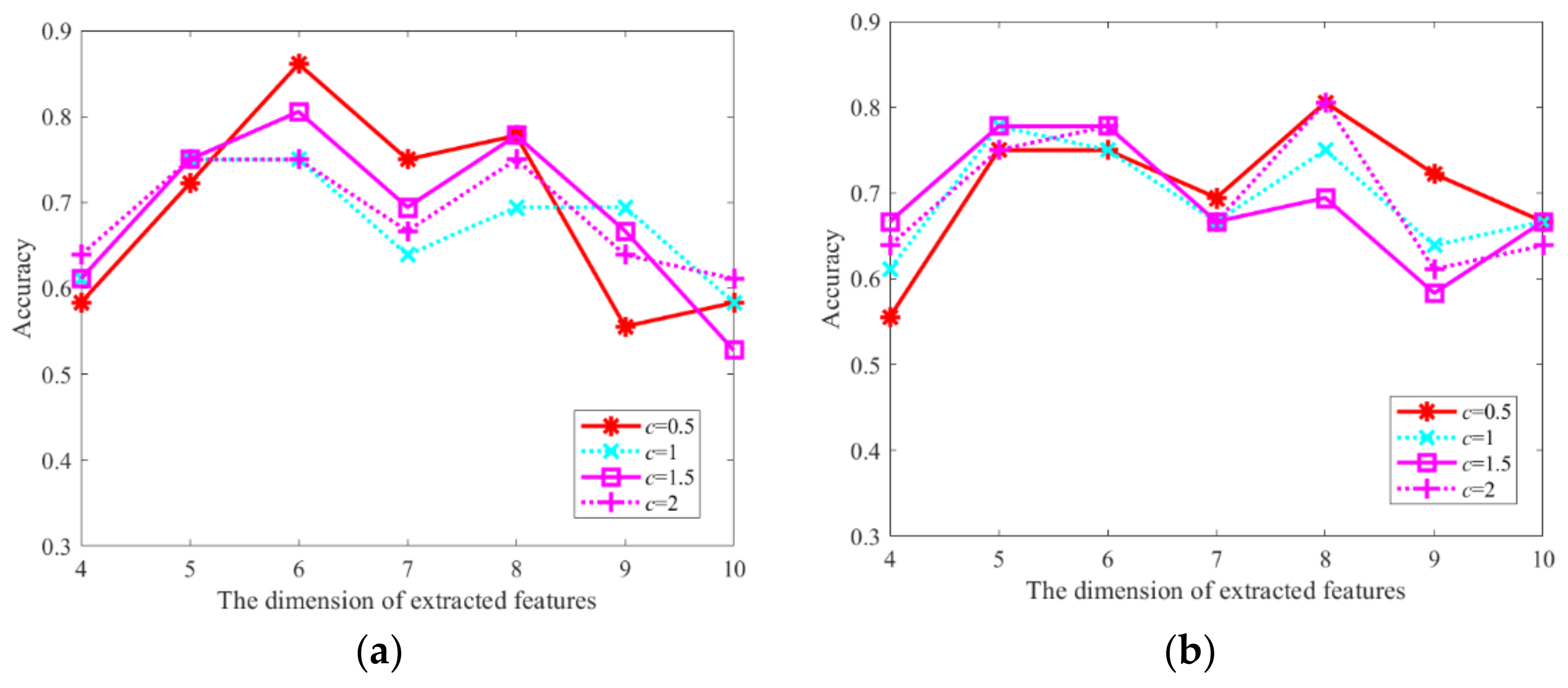
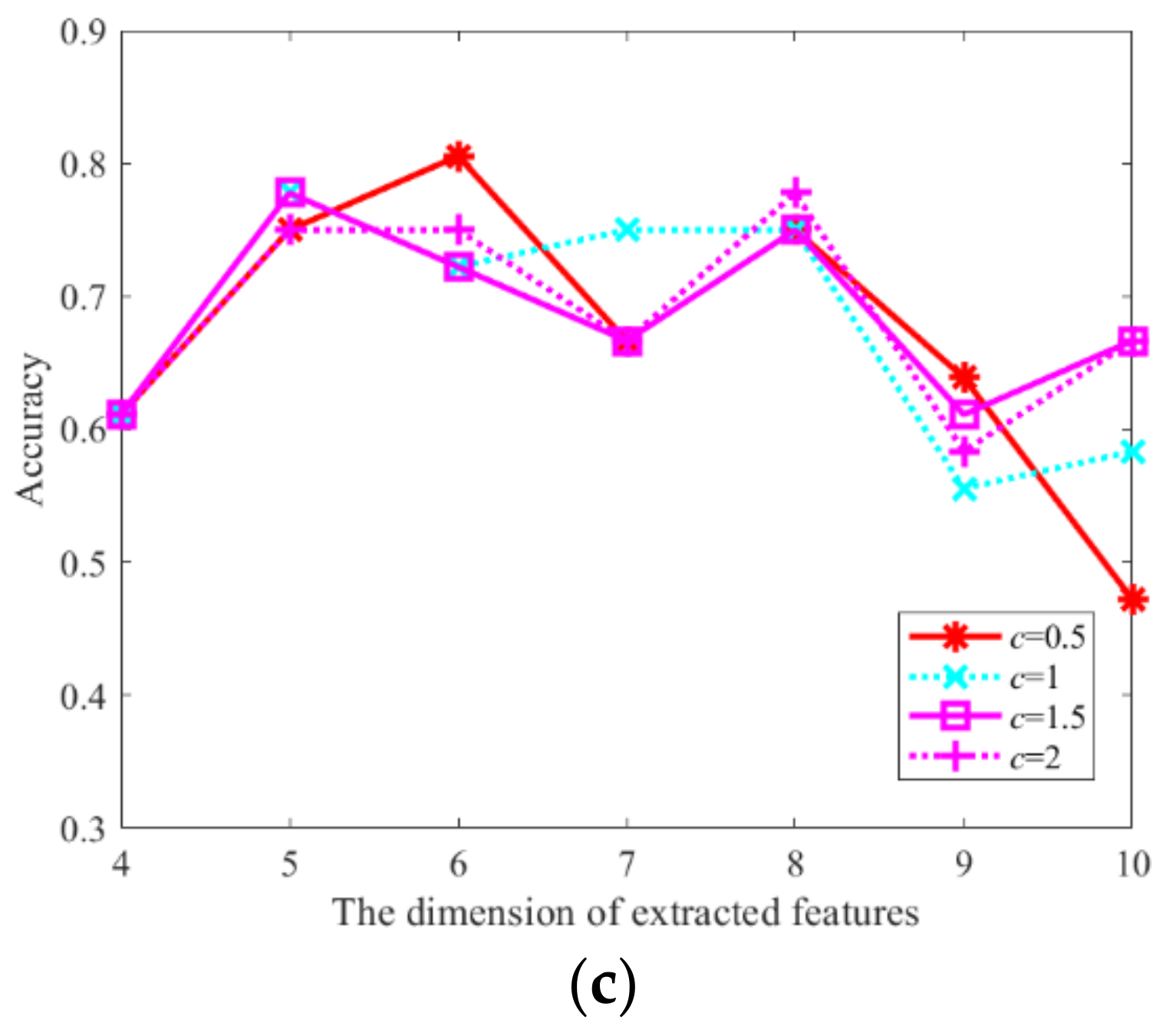
3.4. Analysis of the Impact of Parameter Setting on CCT-HTD
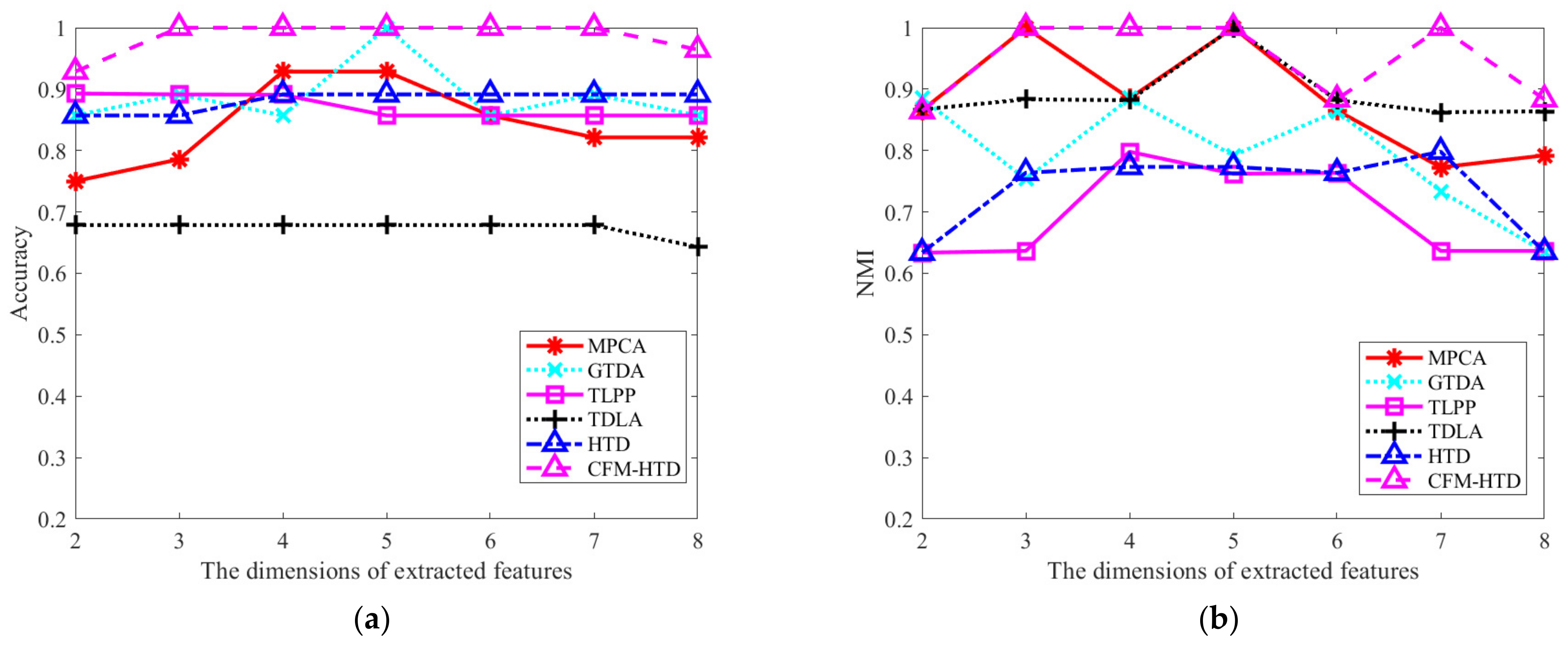
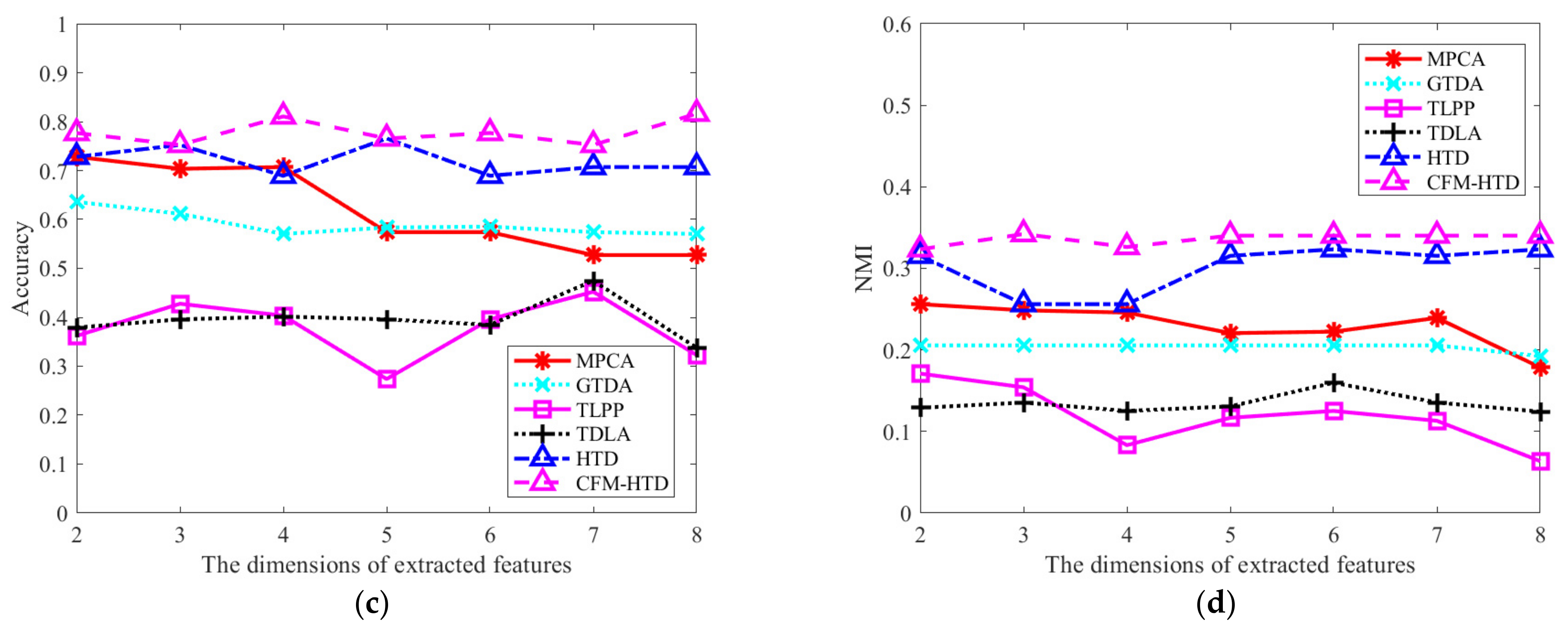
3.5. Evaluation of the Performance of CFM-HTD Compared with Typical Multisource Fusion Methods
3.6. Evaluation of the Performance of CCT-HTD Compared with Typical Domain Adaptation Methods
4. Discussion
4.1. Discussion of the Experimental Results of the Proposed Methods
4.2. Discussion of the Relationship between Coupled Heterogeneous Tucker Decomposition and the Existing Methods
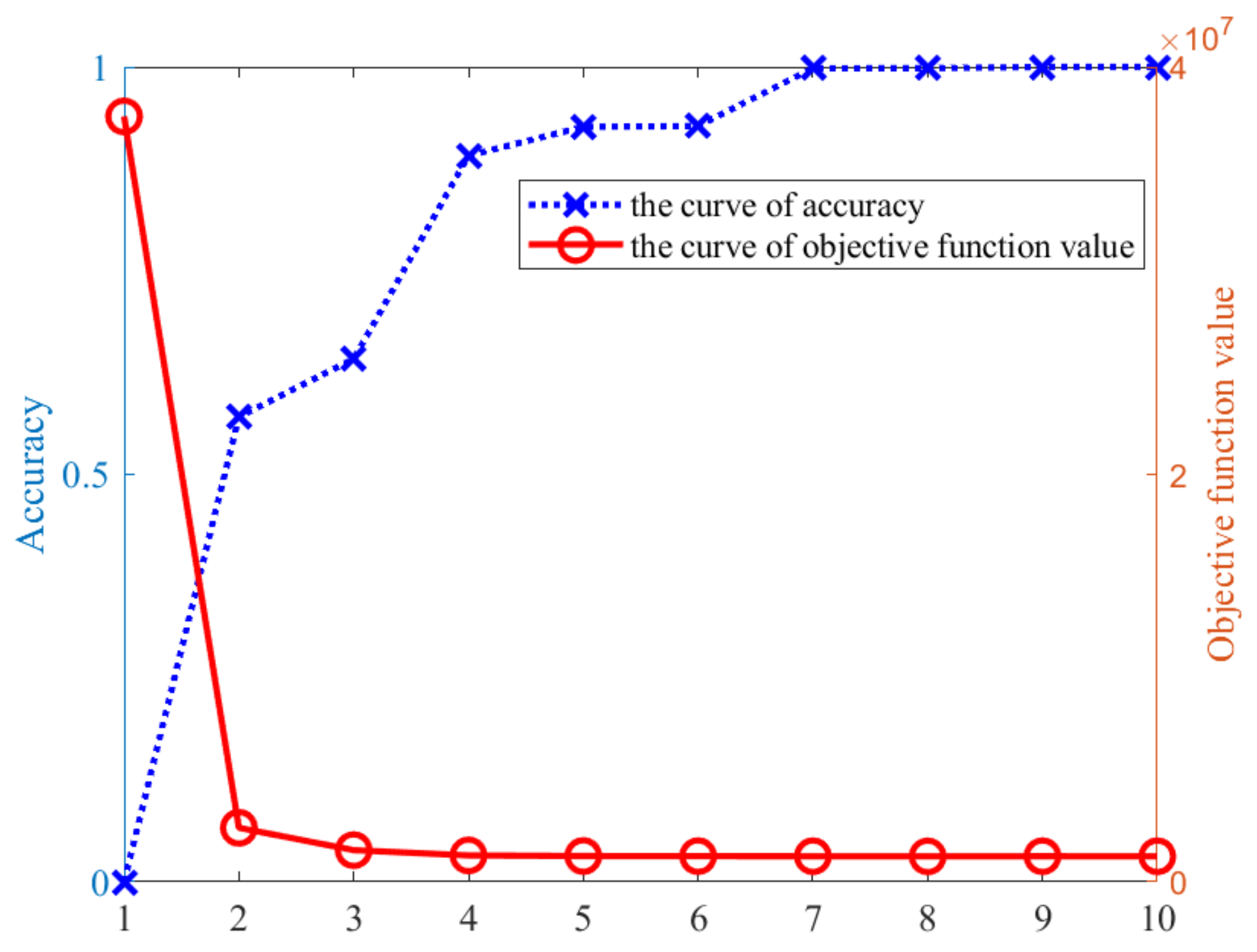
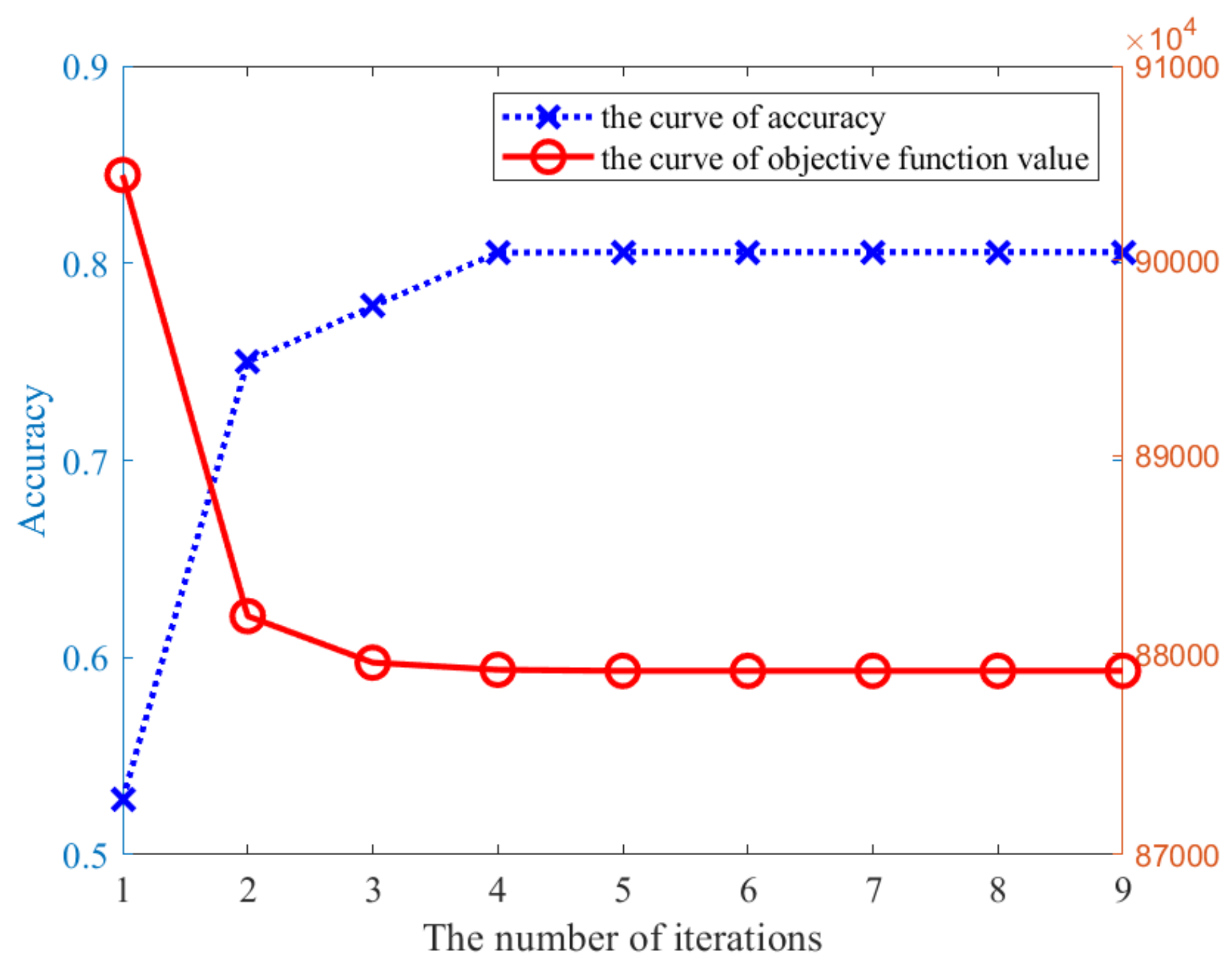
4.3. Discussion of the Convergence and Complexity
5. Conclusions
Supplementary Materials
Author Contributions
Funding
Data Availability Statement
Conflicts of Interest
Appendix A
References
- Mahmoudi, F.T.; Samadzadegan, F.; Reinartz, P. Object recognition based on the context aware decision-level fusion in multiviews imagery. IEEE J. Sel. Top. Appl. Earth Obs. Remote Sens. 2014, 8, 12–22. [Google Scholar] [CrossRef] [Green Version]
- Wu, B.; Sun, X.; Wu, Q.; Yan, M.; Wang, H.; Fu, K. Building reconstruction from high-resolution multiview aerial imagery. IEEE Geosci. Remote Sens. Lett. 2014, 12, 855–859. [Google Scholar]
- Sumbul, G.; Cinbis, R.G.; Aksoy, S. Multisource region attention network for fine-grained object recognition in remote sensing imagery. IEEE Trans. Geosci. Remote Sens. 2019, 57, 4929–4937. [Google Scholar] [CrossRef]
- Karachristos, K.; Koukiou, G.; Anastassopoulos, V. Fully Polarimetric Land Cover Classification Based on Hidden Markov Models Trained with Multiple Observations. Adv. Remote Sens. 2021, 10, 102–114. [Google Scholar] [CrossRef]
- Koukiou, G.; Anastassopoulos, V. Fully Polarimetric Land Cover Classification Based on Markov Chains. Adv. Remote Sens. 2021, 10, 47–65. [Google Scholar] [CrossRef]
- Jolliffe, I.T. Springer series in statistics. In Principal Component Analysis; Springer: New York, NY, USA, 2002; p. 29. [Google Scholar]
- Martinez, A.M.; Kak, A.C. Pca versus lda. IEEE Trans. Pattern Anal. Mach. Intell. 2001, 23, 228–233. [Google Scholar] [CrossRef] [Green Version]
- Zhang, Q.; Tian, Y.; Yang, Y.; Pan, C. Automatic spatial–spectral feature selection for hyperspectral image via discriminative sparse multimodal learning. IEEE Trans. Geosci. Remote Sens. 2014, 53, 261–279. [Google Scholar] [CrossRef]
- Yang, M.-S.; Sinaga, K.P. A feature-reduction multi-view k-means clustering algorithm. IEEE Access 2019, 7, 114472–114486. [Google Scholar] [CrossRef]
- Pan, S.J.; Tsang, I.W.; Kwok, J.T.; Yang, Q. Domain adaptation via transfer component analysis. IEEE Trans. Neural Netw. 2010, 22, 199–210. [Google Scholar] [CrossRef] [Green Version]
- Gretton, A.; Borgwardt, K.M.; Rasch, M.J.; Schölkopf, B.; Smola, A. A kernel two-sample test. J. Mach. Learn. Res. 2012, 13, 723–773. [Google Scholar]
- Long, M.; Wang, J.; Ding, G.; Sun, J.; Yu, P.S. Transfer feature learning with joint distribution adaptation. In Proceedings of the IEEE International Conference on Computer Vision, Sydney, Australia, 1–8 December 2013; pp. 2200–2207. [Google Scholar]
- Peng, Z.; Zhang, W.; Han, N.; Fang, X.; Kang, P.; Teng, L. Active transfer learning. IEEE Trans. Circuits Syst. Video Technol. 2019, 30, 1022–1036. [Google Scholar] [CrossRef] [Green Version]
- Liu, Y.; Tu, W.; Du, B.; Zhang, L.; Tao, D. Homologous component analysis for domain adaptation. IEEE Trans. Image Process. 2019, 29, 1074–1089. [Google Scholar] [CrossRef] [PubMed]
- Tucker, L.R. Implications of factor analysis of three-way matrices for measurement of change. Probl. Meas. Change 1963, 15, 3. [Google Scholar]
- Harshman, R.A. Foundations of the PARAFAC Procedure: Models and Conditions for an “Explanatory” Multimodal Factor Analysis; University Microfilms: Ann Arbor, MI, USA, 1970. [Google Scholar]
- Lu, H.; Plataniotis, K.N.; Venetsanopoulos, A.N. MPCA: Multilinear principal component analysis of tensor objects. IEEE Trans. Neural Netw. 2008, 19, 18–39. [Google Scholar]
- Tao, D.; Li, X.; Wu, X.; Maybank, S.J. General tensor discriminant analysis and gabor features for gait recognition. IEEE Trans. Pattern Anal. Mach. Intell. 2007, 29, 1700–1715. [Google Scholar] [CrossRef]
- Zheng, D.; Du, X.; Cui, L. Tensor locality preserving projections for face recognition. In Proceedings of the 2010 IEEE International Conference on Systems, Man and Cybernetics, Istanbul, Turkey, 10–13 October 2010; pp. 2347–2350. [Google Scholar]
- Zhang, L.; Zhang, L.; Tao, D.; Huang, X. Tensor discriminative locality alignment for hyperspectral image spectral–spatial feature extraction. IEEE Trans. Geosci. Remote Sens. 2012, 51, 242–256. [Google Scholar] [CrossRef]
- Sun, Y.; Gao, J.; Hong, X.; Mishra, B.; Yin, B. Heterogeneous tensor decomposition for clustering via manifold optimization. IEEE Trans. Pattern Anal. Mach. Intell. 2015, 38, 476–489. [Google Scholar] [CrossRef] [Green Version]
- Sun, B.; Feng, J.; Saenko, K. Correlation alignment for unsupervised domain adaptation. In Domain Adaptation in Computer Vision Applications; Springer: Berlin/Heidelberg, Germany, 2017; pp. 153–171. [Google Scholar]
- Jia, S.; Liu, X.; Xu, M.; Yan, Q.; Zhou, J.; Jia, X.; Li, Q. Gradient feature-oriented 3-D domain adaptation for hyperspectral image classification. IEEE Trans. Geosci. Remote Sens. 2021, 60, 1–17. [Google Scholar] [CrossRef]
- Gao, G.; Gu, Y. Tensorized principal component alignment: A unified framework for multimodal high-resolution images classification. IEEE Trans. Geosci. Remote Sens. 2018, 57, 46–61. [Google Scholar] [CrossRef]
- Tao, D.; Li, X.; Wu, X.; Hu, W.; Maybank, S.J. Supervised tensor learning. Knowl. Inf. Syst. 2007, 1, 1–42. [Google Scholar] [CrossRef]
- Ma, Z.; Yang, L.T.; Zhang, Q. Support Multimode Tensor Machine for Multiple Classification on Industrial Big Data. IEEE Trans. Ind. Inf. 2020, 17, 3382–3390. [Google Scholar] [CrossRef]
- Rosenstein, M.T.; Marx, Z.; Kaelbling, L.P.; Dietterich, T.G. To Transfer or Not to Transfer. In Proceedings of the NIPS: 2005. Workshop on Transfer Learning, Vancouver, BC, Canada, 5–8 December 2005. [Google Scholar]
- Kolda, T.G.; Bader, B.W. Tensor decompositions and applications. SIAM Rev. 2009, 51, 455–500. [Google Scholar] [CrossRef]
- De Lathauwer, L.; De Moor, B.; Vandewalle, J. A multilinear singular value decomposition. SIAM J. Matrix Anal. Appl. 2000, 21, 1253–1278. [Google Scholar] [CrossRef] [Green Version]
- De Lathauwer, L.; De Moor, B.; Vandewalle, J. On the best rank-1 and rank-(r 1, r 2,..., rn) approximation of higher-order tensors. SIAM J. Matrix Anal. Appl. 2000, 21, 1324–1342. [Google Scholar] [CrossRef]
- Higham, N.; Papadimitriou, P. Matrix Procrustes Problems; Rapport technique; University of Manchester: Manchester, UK, 1995. [Google Scholar]
- Boyd, S.; Parikh, N.; Chu, E.; Peleato, B.; Eckstein, J. Distributed optimization and statistical learning via the alternating direction method of multipliers. Found. Trends Mach. Learn. 2011, 3, 1–122. [Google Scholar] [CrossRef]
- Ross, T.D.; Worrell, S.W.; Velten, V.J.; Mossing, J.C.; Bryant, M.L. Standard SAR ATR evaluation experiments using the MSTAR public release data set. In Proceedings of the Algorithms for Synthetic Aperture Radar Imagery V, Orlando, FL, USA, 15 September 1998; pp. 566–573. [Google Scholar]
- Zhang, L.; Zhang, L.; Tao, D.; Huang, X. A multifeature tensor for remote-sensing target recognition. IEEE Geosci. Remote Sens. Lett. 2010, 8, 374–378. [Google Scholar] [CrossRef]
- Gonzalez, R.C. Digital Image Processing; Pearson Education India: Chennai, Indian, 2009. [Google Scholar]
- Cameron, W.L.; Rais, H. Derivation of a signed Cameron decomposition asymmetry parameter and relationship of Cameron to Huynen decomposition parameters. IEEE Trans. Geosci. Remote Sens. 2011, 49, 1677–1688. [Google Scholar] [CrossRef]
- Touzi, R. Target scattering decomposition in terms of roll-invariant target parameters. IEEE Trans. Geosci. Remote Sens. 2006, 45, 73–84. [Google Scholar] [CrossRef]
- Van der Maaten, L.; Hinton, G. Visualizing data using t-SNE. J. Mach. Learn. Res. 2008, 9, 2579–2605. [Google Scholar]
- Roweis, S.T.; Saul, L.K. Nonlinear dimensionality reduction by locally linear embedding. Science 2000, 290, 2323–2326. [Google Scholar] [CrossRef] [PubMed] [Green Version]
- Belkin, M.; Niyogi, P. Laplacian eigenmaps for dimensionality reduction and data representation. Neural Comput. 2003, 15, 1373–1396. [Google Scholar] [CrossRef] [Green Version]
- Tian, L.; Tang, Y.; Hu, L.; Ren, Z.; Zhang, W. Domain adaptation by class centroid matching and local manifold self-learning. IEEE Trans. Image Process. 2020, 29, 9703–9718. [Google Scholar] [CrossRef] [PubMed]
- Hu, W.; Kong, X.; Xie, L.; Yan, H.; Qin, W.; Meng, X.; Yan, Y.; Yin, E. Joint Feature-Space and Sample-Space Based Heterogeneous Feature Transfer Method for Object Recognition Using Remote Sensing Images with Different Spatial Resolutions. Sensors 2021, 21, 7568. [Google Scholar] [CrossRef] [PubMed]
- Cortes, C.; Vapnik, V. Support-vector networks. Mach. Learn. 1995, 20, 273–297. [Google Scholar] [CrossRef]
- Peng, W. Constrained nonnegative tensor factorization for clustering. In Proceedings of the 2010 Ninth International Conference on Machine Learning and Applications, Washington, DC, USA, 12–14 December 2010; pp. 954–957. [Google Scholar]


| Satellite | Roll Angle | Resolution | Acquired Time |
|---|---|---|---|
| SuperView-1 | −2.79° | 0.5 m | 9 February 2020 |
| SuperView-1 | −13.62° | 0.5 m | 30 July 2020 |
| Jilin-1 | 33.11° | 1 m | 7 October 2020 |
| Jilin-1 | −34.20° | 1 m | 7 November 2020 |
| PCA | LLE | LE | MPCA | HTD | GTDA | TLPP | TDLA | CFM-HTD | |
|---|---|---|---|---|---|---|---|---|---|
| NMI | 0.769 | 0.184 | 0.200 | 0.8633 | 0.7981 | 0.8827 | 0.7984 | 0.8827 | 1 |
| ACC | 0.75 | 0.6071 | 0.6786 | 0.9286 | 0.8929 | 0.8929 | 0.6786 | 1 | 1 |
| PCA | LLE | LE | MPCA | HTD | GTDA | TLPP | TDLA | CFM-HTD | |
|---|---|---|---|---|---|---|---|---|---|
| NMI | 0.2159 | 0.1423 | 0.0797 | 0.2556 | 0.3234 | 0.2063 | 0.1715 | 0.1598 | 0.3403 |
| ACC | 0.7288 | 0.5876 | 0.4832 | 0.7232 | 0.7655 | 0.6384 | 0.4520 | 0.4746 | 0.7797 |
| PCA | LLE | LE | MPCA | HTD | GTDA | TLPP | TDLA | CFM-HTD | |
|---|---|---|---|---|---|---|---|---|---|
| NMI | 0.2496 | 0.1992 | 0.2166 | 0.2199 | 0.3365 | 0.2762 | 0.2596 | 0.3885 | 0.4052 |
| ACC | 0.7742 | 0.6452 | 0.6774 | 0.8065 | 0.8338 | 0.7419 | 0.7419 | 0.8710 | 0.8710 |
| Classifier | Task | PCA | HTD | TCA | CORAL | JDA | ATL | CMMS | JFSSS-HFT | CCT-HTD |
|---|---|---|---|---|---|---|---|---|---|---|
| 1NN | 47.2% | 52.78% | 77.8% | 50% | 63.89% | 52.78% | 52.78% | 83.3% | 86.1% | |
| 47.7% | 53.85% | 49.3% | 47.7% | 49.2% | 46.2% | 52.3% | 83.1% | 84.62 | ||
| SVM | 58.33% | 50% | 80.56% | 55.56% | 69.44% | 55.56% | 55.56% | 86.1% | 86.1% | |
| 49.3% | 50.77% | 67.7% | 46.2% | 55.4% | 49.2% | 49.2% | 78.5% | 83.08% |
| Classifier | Task | PCA | HTD | TCA | CORAL | JDA | ATL | CMMS | JFSSS-HFT | CCT-HTD |
|---|---|---|---|---|---|---|---|---|---|---|
| 1NN | 59.89% | 49.15% | 61.58% | 58.19% | 68.93% | 59.89% | 72.88% | 66.67% | 73.45% | |
| 59.89% | 51.41% | 59.32% | 20.90% | 59.32% | 40.68% | 68.30% | 61.02% | 71.19% | ||
| SVM | 52.54% | 51.41% | 62.15% | 24.29% | 55.37% | 48.02% | 80.79% | 51.89% | 81.92% | |
| 44.63% | 48.59% | 51.97% | 16.38% | 52.54% | 42.94% | 78.53% | 51.97% | 80.79% |
| Classifier | Task | PCA | HTD | TCA | CORAL | JDA | ATL | CMMS | JFSSS-HFT | CCT-HTD |
|---|---|---|---|---|---|---|---|---|---|---|
| 1NN | 38.71% | 35.48% | 41.94% | 48.39% | 32.26% | 48.39% | 54.84% | 58.06% | 61.29% | |
| 45.16% | 41.94% | 54.84% | 32.26% | 54.84% | 51.61% | 58.06% | 51.61% | 61.29% | ||
| SVM | 48.39% | 48.39% | 41.94% | 29.03% | 48.39% | 48.39% | 58.06% | 61.29% | 64.62% | |
| 54.84% | 48.39% | 54.84% | 25.81% | 51.61% | 51.61% | 51.61% | 58.06% | 67.74% |
| Classifier | Task | PCA | HTD | TCA | CORAL | JDA | ATL | CMMS | JFSSS-HFT | CCT-HTD |
|---|---|---|---|---|---|---|---|---|---|---|
| 1NN | 30.56% | 47.22% | 77.8% | 44.4% | 50% | 50% | 47.22% | 66.67% | 83.3% | |
| 47.7% | 47.69% | 33.85% | 47.7% | 44.62% | 69.27% | 64.62% | 76.92% | 84.62 | ||
| SVM | 41.67% | 50% | 80.56% | 41.67% | 55.56% | 55.56% | 52.78% | 72.2% | 83.3% | |
| 49.3% | 46.15% | 67.7% | 46.2% | 55.4% | 52.3% | 52.31% | 78.5% | 83.08% |
| Classifier | Task | PCA | HTD | TCA | CORAL | JDA | ATL | CMMS | JFSSS-HFT | CCT-HTD |
|---|---|---|---|---|---|---|---|---|---|---|
| 1NN | 39.25% | 45.76% | 59.02% | 56.83% | 56.83% | 48.63% | 65.57% | 49.18% | 73.45% | |
| 24.19% | 45.20% | 56.99% | 19.35% | 63.98% | 27.96% | 69.35% | 57.53% | 70.43% | ||
| SVM | 30.11% | 46.89% | 49.46% | 20.90% | 50.82% | 44.26% | 78.53% | 38.79% | 80.79% | |
| 25.27% | 45.76% | 58.60% | 15.59% | 52.35% | 24.19% | 67.74% | 46.77% | 79.66% |
Publisher’s Note: MDPI stays neutral with regard to jurisdictional claims in published maps and institutional affiliations. |
© 2022 by the authors. Licensee MDPI, Basel, Switzerland. This article is an open access article distributed under the terms and conditions of the Creative Commons Attribution (CC BY) license (https://creativecommons.org/licenses/by/4.0/).
Share and Cite
Gao, T.; Chen, H.; Lu, J. Coupled Heterogeneous Tucker Decomposition: A Feature Extraction Method for Multisource Fusion and Domain Adaptation Using Multisource Heterogeneous Remote Sensing Data. Remote Sens. 2022, 14, 2553. https://doi.org/10.3390/rs14112553
Gao T, Chen H, Lu J. Coupled Heterogeneous Tucker Decomposition: A Feature Extraction Method for Multisource Fusion and Domain Adaptation Using Multisource Heterogeneous Remote Sensing Data. Remote Sensing. 2022; 14(11):2553. https://doi.org/10.3390/rs14112553
Chicago/Turabian StyleGao, Tong, Hao Chen, and Junhong Lu. 2022. "Coupled Heterogeneous Tucker Decomposition: A Feature Extraction Method for Multisource Fusion and Domain Adaptation Using Multisource Heterogeneous Remote Sensing Data" Remote Sensing 14, no. 11: 2553. https://doi.org/10.3390/rs14112553