
Application of Convolutional Neural Networks on Digital Terrain Models for Analyzing Spatial Relations in Archaeology


1
Geomatics Group, Geography Department, Ruhr University Bochum, 44801 Bochum, Germany
2
LWL-Archaeology for Westphalia, 48157 Münster, Germany
*
Author to whom correspondence should be addressed.
Remote Sens. 2022, 14(11), 2535; https://doi.org/10.3390/rs14112535
Submission received: 2 May 2022
/
Revised: 19 May 2022
/
Accepted: 23 May 2022
/
Published: 25 May 2022
(This article belongs to the Special Issue Advances in Remote Sensing for Exploring Ancient History)
Abstract
:Archaeological research is increasingly embedding individual sites in archaeological contexts and aims at reconstructing entire historical landscapes. In doing so, it benefits from technological developments in the field of archaeological prospection over the last 20 years, including LiDAR-based Digital Terrain Models, special visualizations, and automated site detection. The latter can generate comprehensive datasets with manageable effort that are useful for answering large-scale archaeological research questions. This article presents a highly automated workflow, in which a Convolutional Neural Network is used to detect burial mounds in the proximity of remotely located hollow ways. Detected mounds are then analyzed with respect to their distribution and a possible spatial relation to hollow ways. The detection works well, produces a reasonable number of results, and achieved a precision of at least 77%. The distribution of mounds shows a clear maximum in the radius of 2000–2500 m. This supports future research such as visibility or cost path analysis.

1. Introduction
Archaeological research is constantly evolving, especially considering the influence of relatively new techniques such as LiDAR-derived Digital Terrain Models (DTM) and computer-assisted visualization and detection approaches. The past was characterized by dating records and establishing typological development series. Nowadays, it is about understanding historical contexts and landscapes [1,2,3,4,5]. How did humans used to live, influence, and interact with their environment? How were settlement clusters (Siedlungskammern, early settlements in small, cleared areas in forests) structured internally and how were they related to each other? Where were farms or settlements located, where was agricultural land located, where were the deceased buried, and how was the unsettled environment used? Reconstruction of settled landscapes is becoming increasingly important to understand how humans and their environment influenced each other.
At this point, it is worth investigating ancient pathways as they connected farms, settlements, and settlement clusters. However, detecting these is difficult as they often used the same routes as modern roads due to non-changing topographical conditions. They used to run, as they do today, where the distance between start and destination is the easiest to overcome. Especially in mountainous areas, there is often hardly any variation.
One aspect of historic landscape reconstruction is to analyze possible spatial relations of different archaeological objects [6], such as pathways and burial mounds. Up to now, only in some cases, researchers could verify that burial mounds were located near and directly related to pathways [7]. The difficulty is to find proof of whether routes were already used when nearby burial mounds were built. In general, pathways are difficult to date. Even if such a structure is excavated according to most modern archaeological methods, often only finds from the last phase of use are recovered. Finds from the time when a route was first used are not to be expected. In some lucky cases, hoards are discovered along pathways. They were hidden by travelers in dangerous situations and were intended to be picked up later. This sometimes did not happen and today, hoards therefore allow to date pathways to a certain time or to prove that they have been used for a long period.
Automated detection approaches can produce extensive data sets of archaeological records on regional scales and therefore allow investigations of spatial distributions of different monument types. Research on automation in archaeological prospection using airborne LiDAR-derived DTM applied different classifiers such as Template Matching [8,9,10], Object-based Image Analysis (OBIA) [11,12,13,14] or Convolutional Neural Networks (CNN). In recent years, CNNs have proven to be powerful tools for detecting different kinds of archaeological objects [15,16,17,18,19,20,21,22]. They repeatedly apply different kernel filters to input images (convolution), that have been known in remote sensing for a long time, e.g., from the field of edge detection. In this aspect, they are related to Template Matching, which only applies one kernel filter in the form of the desired structure. While training, a CNN observes, which filters intensify or weaken certain structures in the training images and assigns given class names to unique signatures of positively and negatively triggered filters (neurons). An unknown image will then be classified into the class with the most similar signature.
This study presents a scalable, automated workflow for investigating spatial relations of different monument types. The first part of which is a burial mound detection using a CNN to investigate if these also work well with Westphalian monument types and terrain data (1). The second part integrates automated detection approaches into current research to investigate how automation can assist research on archaeological sites within their respective historical contexts (2). In this study, the suspected spatial relation of burial mounds and pathways is evaluated using basic measurements to estimate, within which distance from pathways human activities are to be expected. This will be the basis for further research.
1.1. Study Area
Pathways do not necessarily leave relief imprints, which is impeding their detection from DTMs. However, in mountainous areas, where topology determined available routes ever since, hollow ways developed along frequently used routes, which were also possibly used longer than pathways in flatlands. This would increase the chance that hollow ways date to the same time as possible mounds in their proximity and make results more reliable. Furthermore, mountainous areas are often forested, which preserves the relief from leveling. Under those conditions, hollow ways, burial mounds, and other relief structures are well visible in a DTM (Figure 1) [23,24].
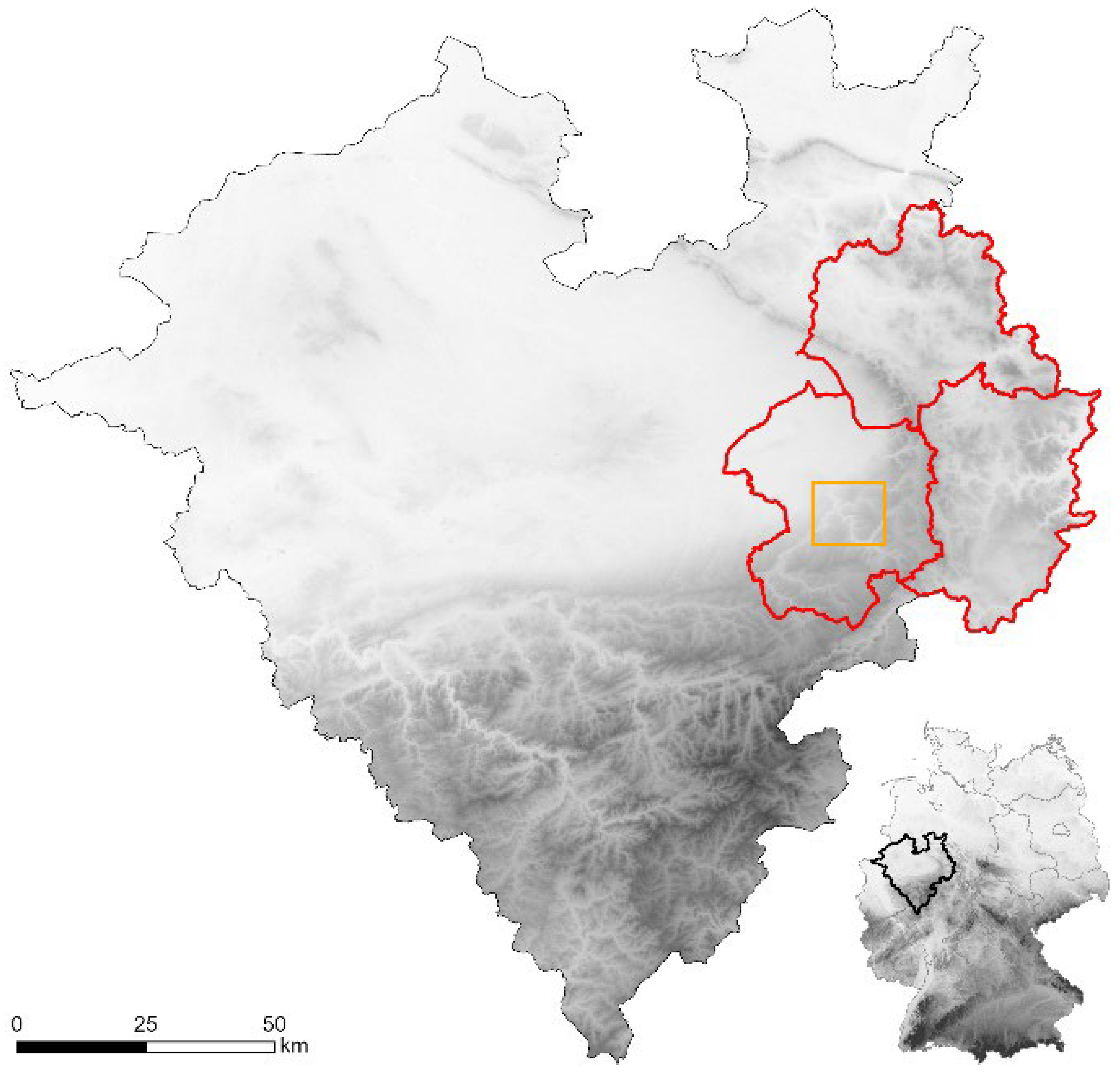
The eastern part of North Rhine-Westphalia, called Westfalen-Lippe, is the area of responsibility of the LWL archaeological institute (Landschaftsverband Westfalen-Lippe, Archäologie für Westfalen, Figure 2). Within this region, several aspects were considered in choosing an adequate study area for this specific study.
- Hollow ways usually appear in mountainous regions as they require certain relief energy.
- Repetitive plowing levels relief features, including above-terrain monuments.
- Only regions that were populated during the Bronze and Iron Age, where most mounds in Westphalia and Lippe date to, are of interest.
- Areas with modern infrastructure are to be rejected as monuments are usually destroyed and new detections probably correspond to modern relief features.
- Forests have a relief-preserving character. Therefore, monuments are most likely to be intact.
Considering all criteria, foremost forests in three regions in East Westphalia and Lippe remain suitable for investigation (Figure 2). The northeastern and central, flat Westphalian Basin (Westfälische Bucht) is unsuitable due to its agricultural character and flat terrain. The same applies to the mountainous area of South Westphalia (Sauerland). According to the current state of research, it was poorly populated in the relevant periods [26].
For training the CNN, a training area of 168 km² was defined (Figure 2) for which reliable reference data are available. It is located directly south of the city of Paderborn in the transition from a rather flat terrain to the Paderborn Plateau, whose surface is cut by river valleys.
1.2. Data
The LiDAR data sets were acquired in 2018 and 2019 and are provided online by the provincial government as filtered last pulse point data in an interpolated regular grid of 1 pt/m² [25]. These data can be converted into a DTM without interpolation and are sufficient for this purpose.
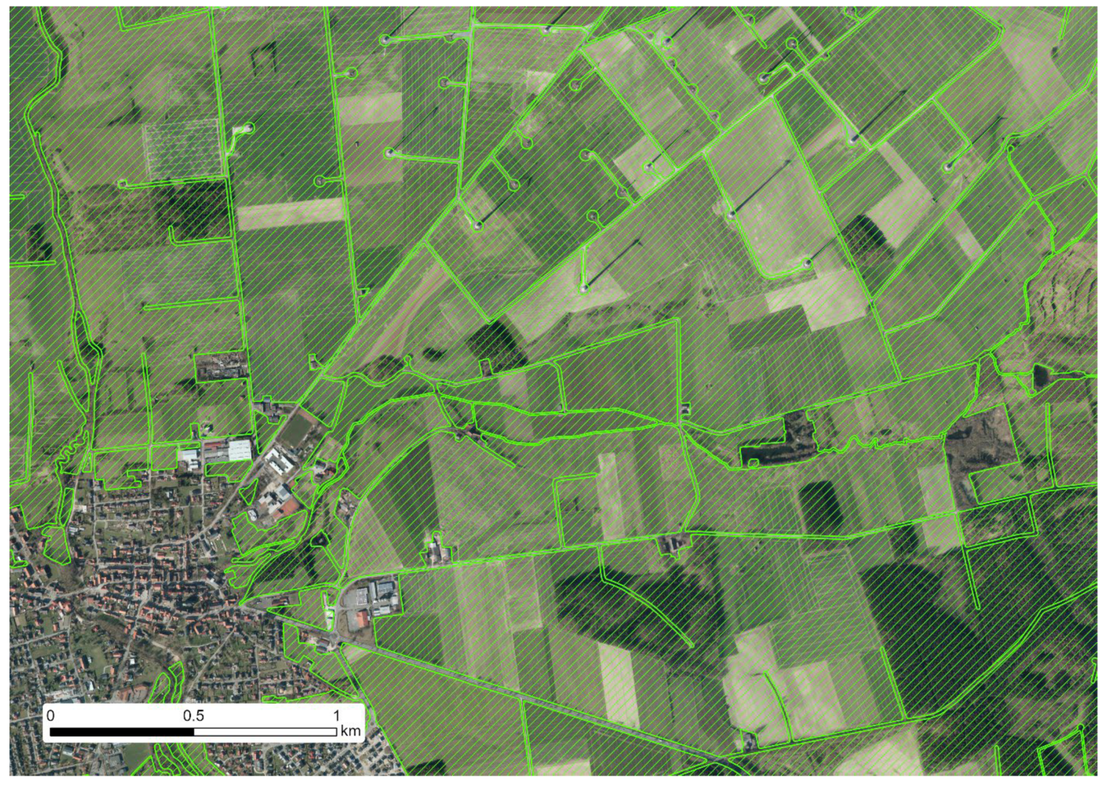
Confusions with modern structures affect both manual and automated classifications of archaeological objects, which is in particular true for simple relief structures such as mounds and pits [12,14,17]. Mounds in forests are more interesting than those in settled areas as they are less likely to be related to modern infrastructure. Location-based ranking is a suitable method for differentiating morphologically identical structures [14,20,28]. This is implemented via the Positive Layer from previous work [29] (Figure 3). During generation, relief imprints of modern infrastructure were estimated and removed from the area of Westphalia and Lippe. Finally, this data set contains areas that are probably not affected and therefore archaeologically relevant. It is used to select hollow ways and to reduce false positives in the classification. Additionally, a governmental forest data set is used to further estimate the remoteness of hollow ways [25].
Data concerning hollow ways and burial mounds were extracted from the LWL database of archaeological records as point vector data. As this database grew over decades and automated detection tools were not available until recently, its data cannot directly serve as a reference for automated detection approaches. Mound clusters are often recorded as a whole. Therefore, the authors ensured that every single mound was represented individually by a centered point geometry. Records of destroyed or completely eroded mounds were removed. After visual inspection, 194 reference mounds were used for training the CNN. This number is not ideal for CNN training. However, access to very high-quality reference data in terms of the issues addressed above is limited.
2. Methodology
Software-wise only ArcGIS Pro 2.9 by ESRI was used as it includes a deep learning infrastructure, whose user-friendly tools grant easy access to deep learning. For time and efficiency reasons, the automated workflow was not run as a whole but was split into a few parts such as preparation and classification. Each of which was automated using the ArcGIS Pro ModelBuilder as that could be used to visualize the workflow at the same time. Unlisted parameters in the corresponding figures were left on default.
To fulfill conditions 4 and 5 of the list above and to estimate the remoteness of hollow ways, the geometric intersection of the Positive Layer and forests was calculated. For every known hollow way in the study area, the portion of archaeologically relevant forests within 500 m was calculated. Only those monuments were considered, that are surrounded by archaeologically relevant forests to an extent of at least 90% and are located in the region described above, leaving a total of 43 monuments. Terrain data were then acquired for circular zones of a 3 km radius around these hollow ways (Figure 4) as well as for the training area.
The acquired terrain point data were directly converted into a raster DTM as the points are already distributed evenly in a 1 m grid and therefore do not require interpolation. From the DTM including absolute height, the following steps generated a 3-band input DTM that the CNN mound classification was based on (Figure 5).
- The initial DTM was smoothed using a circular filter of a 1 m radius to reduce noise.
- Sinks were removed. In slope maps, mounds and sinks look alike as slope values are not indicating upwards or downwards trends. Filling sinks should ease the training process of the CNN.
- The purged DTM was then used to calculate three visualizations that describe mounds in their respective way:
- Aspect: mounds are represented by a unique composition of all available aspects in one place, looking like an umbrella if classified conventionally in 8 cardinal directions (D8).
- Slope: mounds appear as ring-shaped slope anomalies.
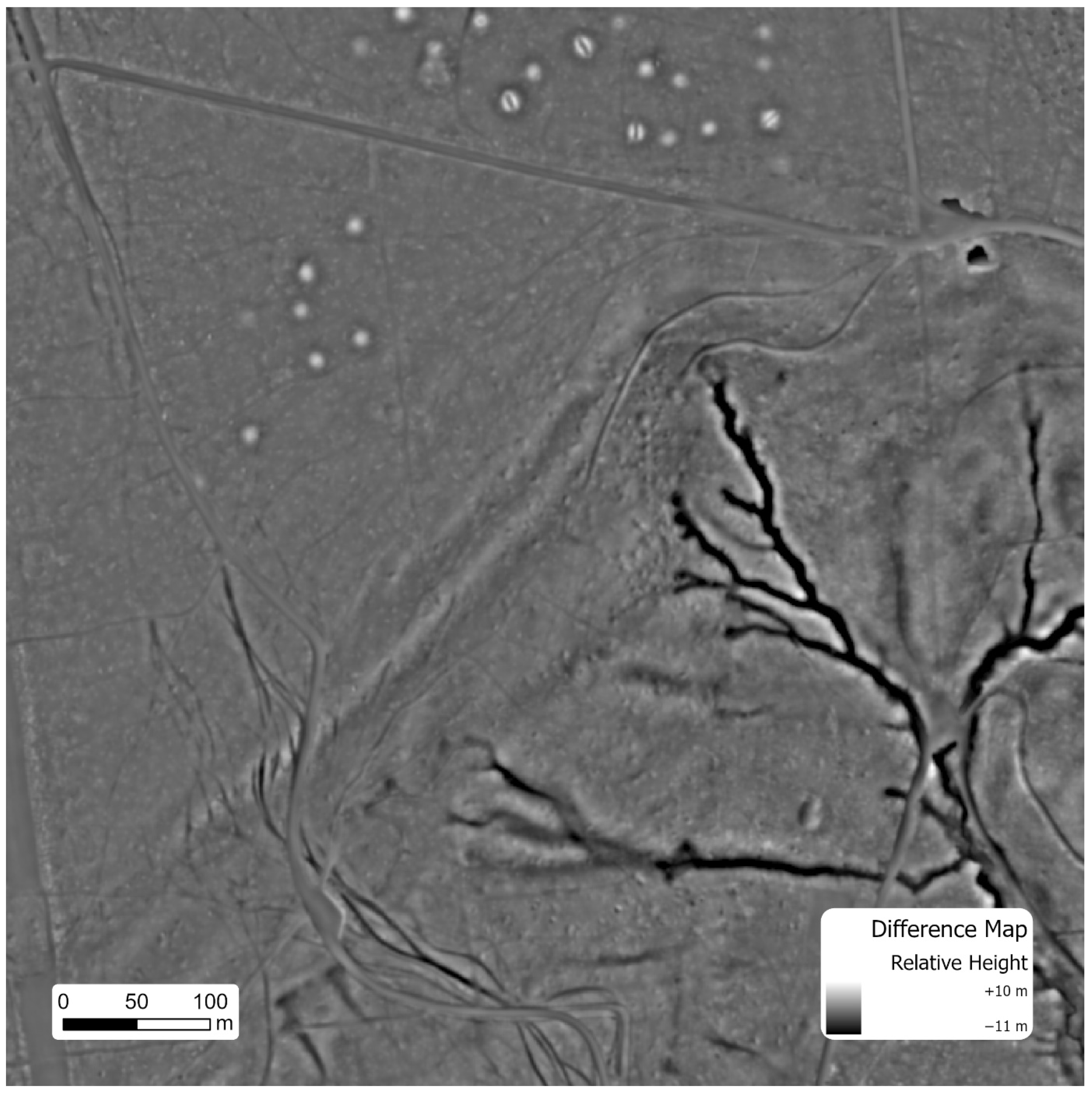
- Difference Map: mounds are described as round local maxima. It is based on trend removal using a circular filter of a radius of 10 m, which corresponds to most known burial mounds. The smoothed DTM including the macro relief was then subtracted from the initial one to extract micro relief features [30].
- These visualizations were finally composed into a 3-band DTM.
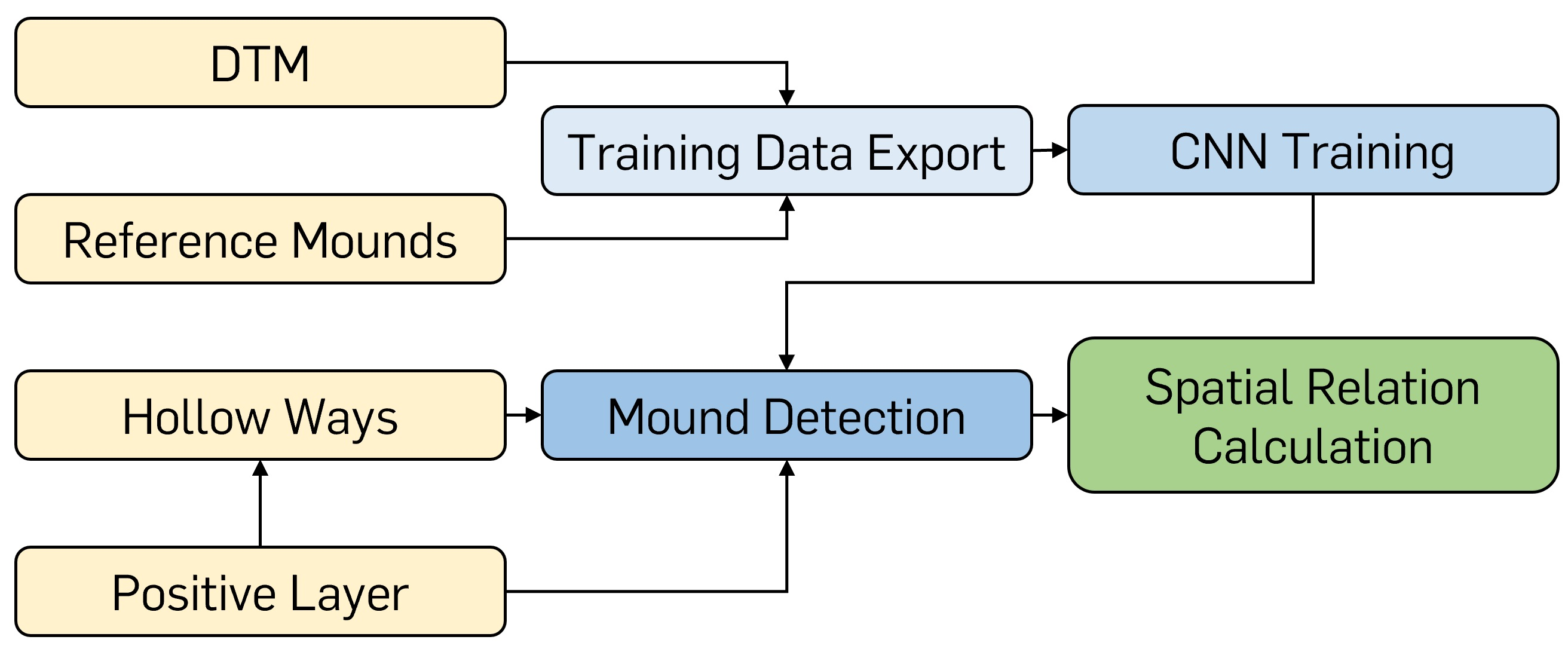
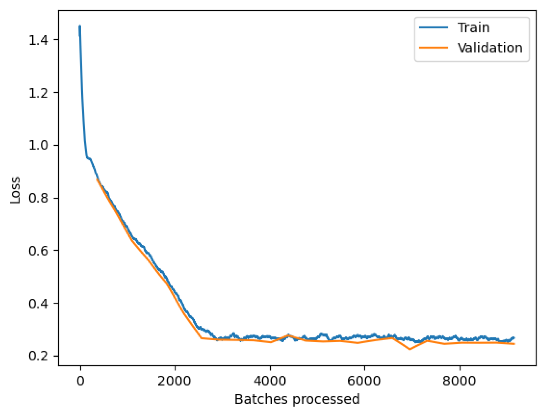
Working with CNNs and other deep learning techniques in this environment consists of three steps: training data generation, training, and detection. A point data set consisting of 194 reference mounds and 219 randomly placed non-mound points was generated. For all points, buffer zones of 12 m radius were calculated. The resulting areas were then used to clip image chips of 30 × 30 pixels from the 3-band DTM using a stride of 15 pixels. To increase the number of chips, a rotation angle of 45° was used, increasing the number of mound samples drastically. In the next step, a Faster R-CNN was trained using a frozen RESNET50 backbone model, a chip size of 175, and an epoch limit of 50 (training stopped after 25 epochs as the model did not further improve). Finally, the CNN was applied to the training area using a threshold of 50%. This is unusually low on purpose to allow a deeper evaluation of the model’s performance (Figure 6 and Figure 7).
On a modern mid-range computer with a Ryzen 3100 8-thread CPU @ 3.90 GHz, 16 GB of RAM, and a GTX 1660 Super (6 GB), the export step took 13 h and 16 min to complete. The authors exaggerated in this case on purpose to investigate the influence of the number of training chips (exports with an angle of 180° only took around 1 h, reducing training time as well). Training then took 2 h and 18 min and detection 1 h and 46 min. The batch_size parameter was maxed out in each step to use available resources as efficiently as possible.
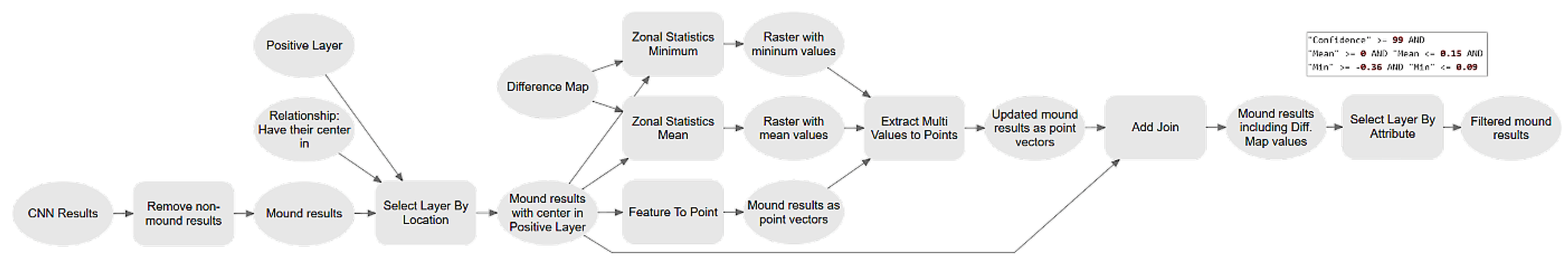
Without post classification (Figure 8), the CNN generated 17,993 results and was able to find 191 of 194 reference mounds (recall: 98.45%). After removing non-mound results, 7210 results were left, including 190 reference mounds (recall: 97.94%). One mound was misclassified, although it served for the generation of image chips. At this stage, precision (true positives/(true positives + false positives)) was not yet reasonable (1.06%/2.64%).
The positive layer removed all results whose center was not located within, as these usually do not represent mounds. This left 3549 results and 186 reference mounds (recall: 95.87%). Some mounds located very close to or crossed by modern infrastructure were removed as well (Figure 9). Raising the confidence threshold to 99% leaves 161 results and 138 detected reference mounds (recall: 71.13%) and produces a reasonable precision of 85.71%. Closer analysis revealed that some results are not false but rather new positives. These are mounds, that the authors did not consider to be suitable for training as they are eroded or damaged and are therefore not representative enough to be part of the training data set. Including them in the calculation would raise precision to 90.68%. It shows that the CNN is generally working well.
These settings turned out to work best for this specific mound detection among other tested configurations. To estimate the influence of training data, first, additional Faster R-CNNs were trained with far less data. The CNNs only performed slightly worse (precision: 88.66%, recall: 44.33%) and using less training data will be considered in future applications, as the extensive 45° data set was generated anyway. Second, the size of training image chips was altered, resulting in worse measurements as well (precision: 68.88%, recall: 69.59%). Mask R-CNNs were tested as well, however, the best performing CNN had an output of only 66 detected mounds at a threshold of 90%. Precision was at only 77.27% and recall at 26.29%.
For the application in unknown regions, the authors consider a high precision to be more important than detecting lots of structures as results should still be interpreted manually. For this specific workflow, the quality therefore is sufficient, as the goal is to produce a manageable number of results that have a high probability to be archaeologically relevant. Therefore, the CNN was applied to a subset of six hollow ways to evaluate transferability and estimate the performance on the whole area(s) of interest (Figure 4). This revealed that additional post classification steps would improve results.
Referring to the principles of OBIA, the output rectangles of the CNN were interpreted as objects, for each of which, the mean and minimum Difference Map pixel values were calculated. Only those were further considered whose mean was ≥0 and ≤0.15 and whose minimum was ≥−0.36 and ≤0.09. These thresholds were determined by manual interpretation of all 348 detections in this area (as reliable reference data are not available). Applying these thresholds only left 12 detections, 9 of which were already included in the database of archaeological records. Three represent probable new detections, meaning that precision is at least 75% while producing a manageable number of results.
Including post classification, the CNN was applied to the whole DTM (Figure 4). Detected mounds were analyzed regarding their spatial distribution around hollow ways. In an iterative process, mounds in areas defined by radii of 500 m to 3000 m were selected and their numbers assigned to the hollow ways (Figure 10).
3. Results
Applied to the whole DTM, the CNN generated 184 output rectangles (Figure 11). About 77 of which were already included in the database of archaeological records. As data for the areas around the hollow ways are probably not complete, the results were interpreted manually to calculate precision at least. This revealed a total of 141 mounds that are to be considered as true positives. The corresponding precision of 77% is already known from the subset. Further, the 43 false positives were investigated regarding the reason for the respective false alarm of the classification. Three of them could be identified as structures that the CNN should not have detected as they are sinks, the exact opposite of mounds. Another eight should have been removed by the Positive Layer as they are modern structures. Some of these are missing in the DLM, others belong to construction sites and are not yet included. The remaining 32 are in fact morphologically identical to burial mounds, e.g., dunes or hilltops. The latter furthermore used to be a welcome location for burial mounds, impeding their isolation even more. The authors observed the same difficulties in another investigation area using OBIA [14].
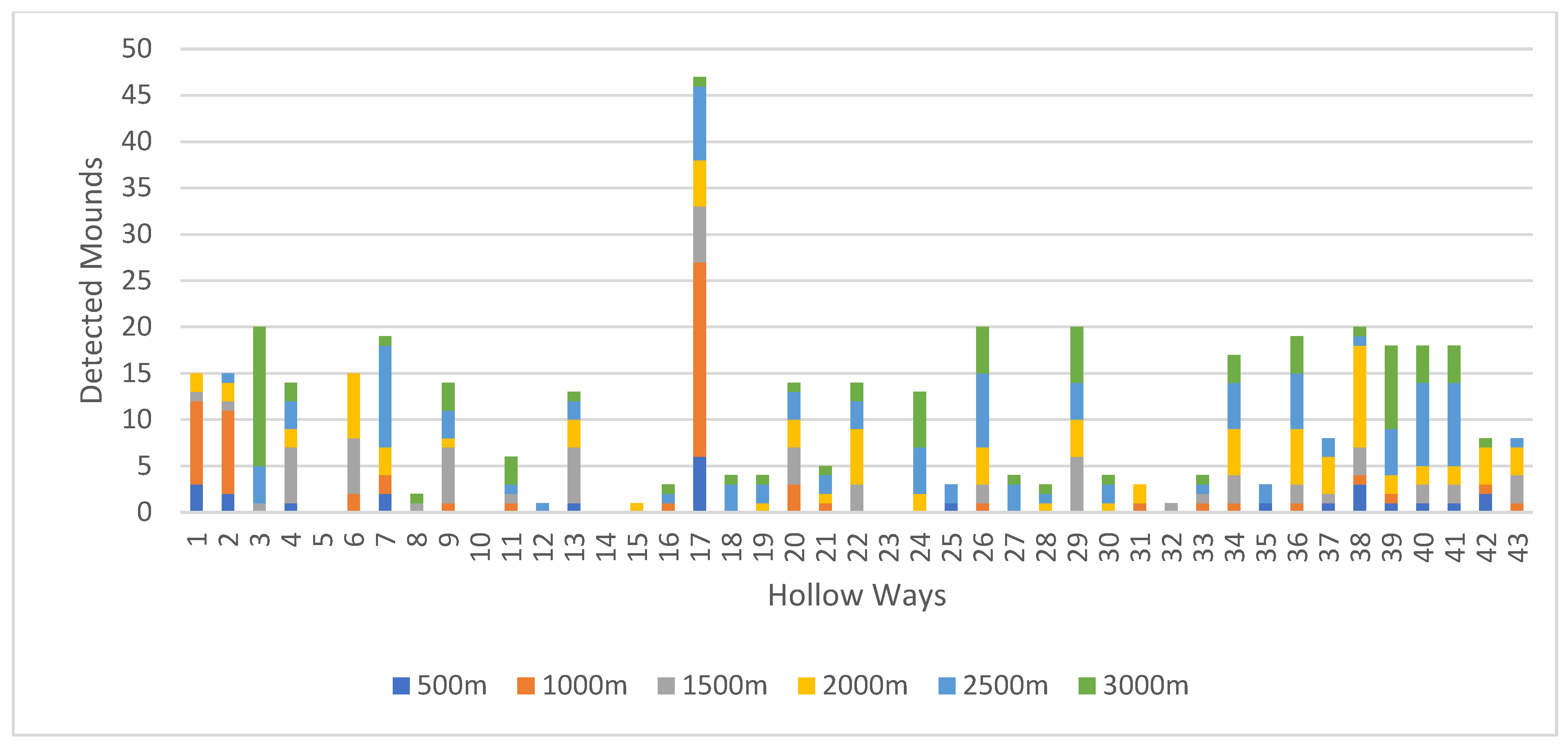
Finally, the number of detected mounds in areas defined by radii of 500 m to 3000 m around each hollow way was calculated (Figure 12 and Table 1).
The combination of the presented hollow way selection and classification allows the following insights and measurements regarding possible spatial relations.
- On the one hand, only 33% of the hollow ways are surrounded by mounds within a radius of 500 m and only 91% within 3000 m. As only very remote locations were considered and archaeological objects should still be existent, the results are probably reliant and hollow ways apparently do not necessarily have mounds around, especially considering that those in a distance of 3000 m are rather unlikely to relate to the observed hollow way. An alternative interpretation is that these hollow ways do not date to an epoch in which burial mounds were built but are younger (Table 1).
- On the other hand, already 72% of the hollow ways have mounds within a distance of 1500 m and 84% within 2000 m. Taking the strict parameters of the (post) classification and weaknesses of the CNN into account, the percentage might actually be higher, which would rather confirm a positive spatial relation. Within this distance, hollow ways are surrounded by two mounds on average (Table 1).
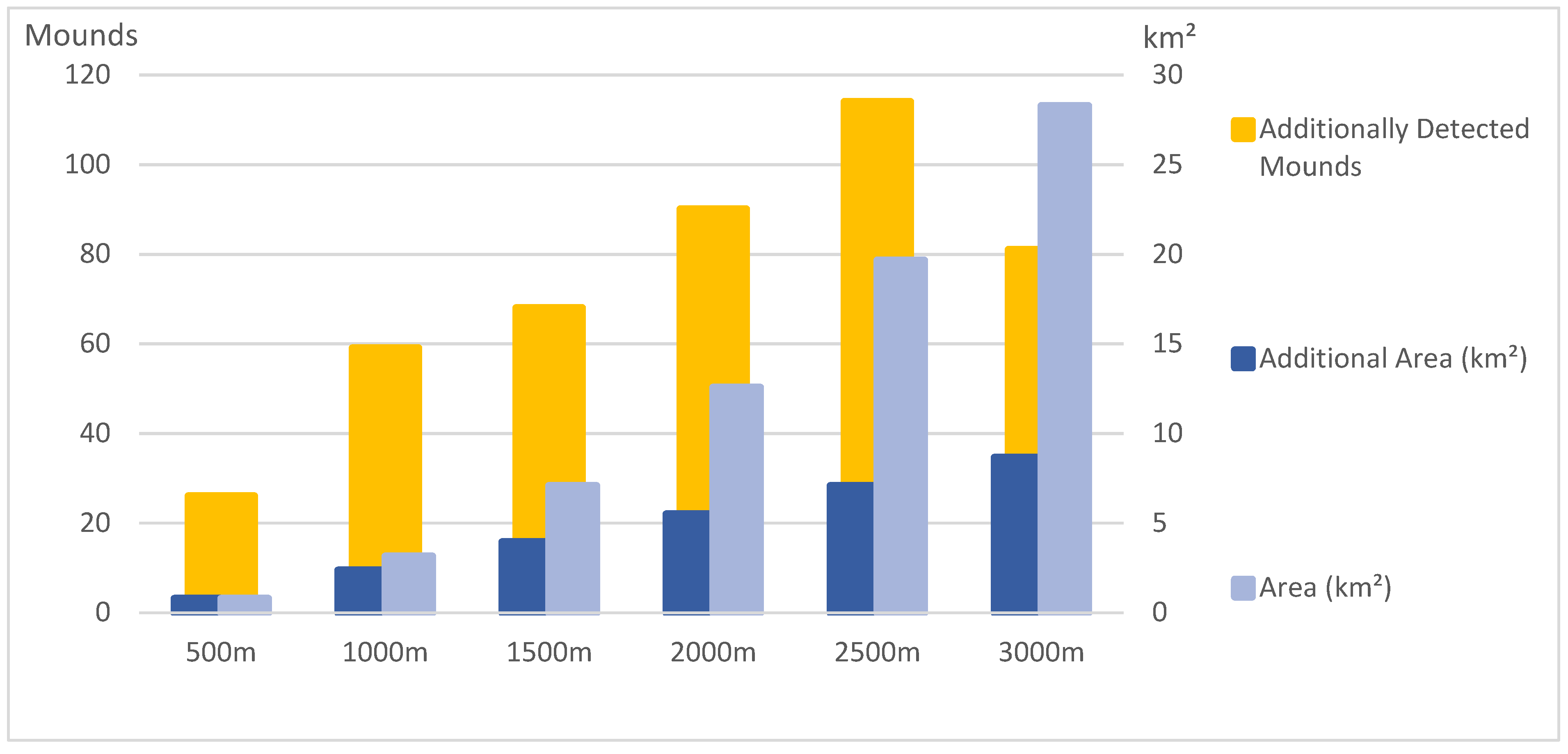
- Corresponding to the basic geographical convention that objects are more related to each other, the closer they are located to one another, the area of investigation around each hollow way should be limited. Furthermore, detections of even larger areas than here require above-average computing resources. As for this study no limit is predefined by archaeological aspects such as visibility or soil type, it is interesting if a meaningful limit can be derived from the data itself.In general, the absolute number of detected mounds increases along with the size of the area around each hollow way. However, the additional (ring-shaped) area compared to the next smaller one also increases due to growing diameters. Thus, the number of additionally detected mounds must also increase to justify larger areas. As long as this is true, increasing the observed area is reasonable. If not, the sweet spot is achieved. Beyond this point, the classification will possibly suffer from including unnecessarily large areas without generating suitable amounts of results and the workflow will become inefficient and unreliable. Here, this is the case at 2500 m as additional detections significantly drop afterward (Figure 13). In some cases, this distance represents the end of forests, which would explain less detections.
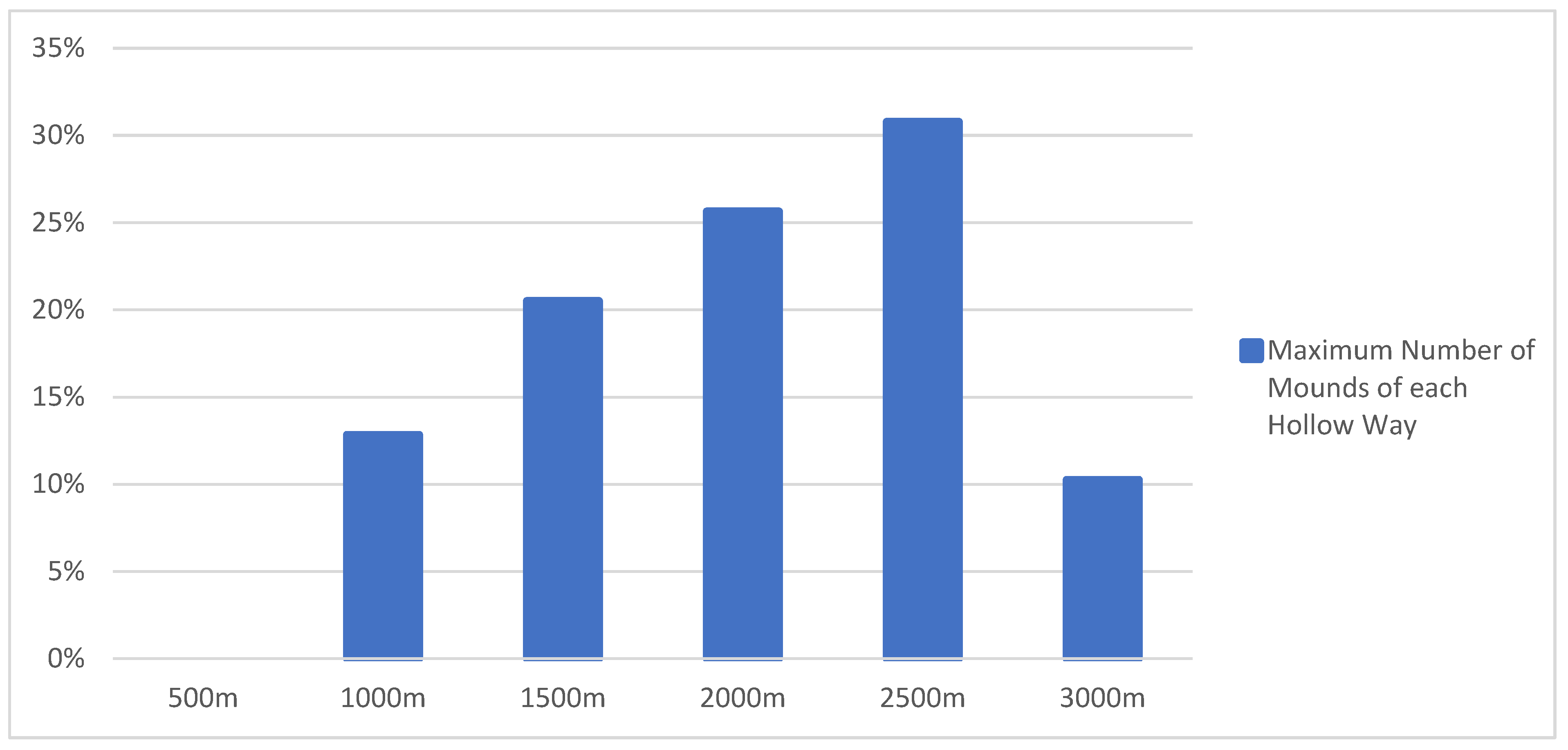
- Analyzing detected mounds around hollow ways as a whole is potentially affected by single hollow ways with large numbers of detections (such as No.17, Table 1). However, considering detected mounds per hollow way allows the same conclusion. No hollow way has its maximum number of mounds within 500 m. For most hollow ways (31%), the area including most mounds is from 2000–2500 m radius, followed by 1500–2000 m (26%) (Figure 14).
- The percentage of hollow ways with a least one mound confirms this as well, as beyond 2500 m, no additional hollow ways appear (91%). In other words: No hollow way has its closest mound within a distance of 2500 m or more (Table 1).
4. Conclusions
The CNN presented useful and reliable performance metrics in the training area. It did not only detect reference mounds but destroyed and eroded mounds as well, which the authors did not consider being part of the reference data set or did not see in the first place. This probably would not have been possible with OBIA as the required object homogeneity is very low.
The application outside the training area revealed that transferability is not naturally given and post classification might be needed. Additionally, the number of detections should be considered when adjusting post classifications parameters. The CNN finally produced useful results, which allow basic insights into spatial relations of hollow ways and burial mounds. Although it was not the focus of this article, the systematic test of different CNNs revealed that Faster R-CNNs outperform Mask R-CNNs by far.
As expected, the Positive Layer also removed some true positives, which is unwanted but is still better than not applying location-based ranking. The amount of training data used here was not necessary, as a significant reduction did not result in equivalently worse results.
The detected mounds could be used for basic spatial relation analysis. To compensate for missed mounds, not only the number of mounds was calculated, but also the distance in which the closed mound is located. This revealed that detection should be limited to 2500 m. Only considering the basic measurements presented above, a spatial relation is far from obvious. Assuming that the results are reliable, not all hollow ways from the Bronze and Iron Age are near burial mounds. An alternative explanation is that not all paths date to these periods.
5. Discussion and Outlook
This study presented a workflow for investigating the spatial relation of hollow ways and burial mounds under rather ideal conditions, under which the workflow itself works well. However, a spatial relation could neither be proven nor denied. More comprehensive and precise applications will be beneficial as the results are dependent on a variety of parameters. Nevertheless, the results reveal guidelines for future applications such as visibility or cost path analysis.
First of which is the selection of hollow ways in terms of the general area of interest as well as regarding the threshold of 90%. The workflow generated useful results and insights under such near-ideal conditions. Future applications of this workflow will reveal its potential under less ideal conditions, and it will be interesting to see, how much of the historic landscape can be reconstructed in such a densely populated region as Westphalia. This will also require more resources in terms of time and computational power. The south of Westphalia was left aside as it was rarely populated in the questionable time. However, this workflow could also be used to verify this. Additionally, the first appearance of hollow ways should be investigated as possibly hollow ways without mounds around date to younger epochs.
The distance categories, in which the number of mounds was counted, are rather arbitrary for now to investigate general trends. Adjusting these to real ancient landscapes, once these become clearer, would be beneficial as the spatial correlation changes within the course of growing radii. The area, in which people used to live and interact, or the visible area around a settlement or hollow way could serve as starting points. The results could also be compared to those of a visibility analysis to investigate, how many mounds in certain proximity can be seen from a specific hollow way. Alternatively, detection could be limited to visible areas.
In technological terms, insights would become more reliable if the CNN would achieve higher precision and recall as then, post classification, if still necessary, could use wider thresholds to detect more results. As the number of training samples was quite low, consequent and repeated generation of training data at locations where the CNN misclassified relief features would be one possible solution. Another parameter is the 3-band DTM, on which this classification is based. E.g., instead of filling the sinks in the original DTM, this could be (additionally) done in the Difference Map as it would consider pseudo structures that are generated by the lowpass filter. For this study, the authors were skeptical about this, as it would have significantly changed the DTM.
Although the application of the Positive Layer not only rejected false positives, it is nevertheless beneficial. Alternatively, only results that are completely within the Positive Layer could be considered (instead of have their center in), which equals stricter class borders. It is possible that more true than false positives are removed. Therefore, the center option was favored in this study as it considers the individual position of a detection. Using the Positive Layer to crop the DTM before detection would probably cut off some archaeological structures but would reduce processing time, especially in situations where hollow ways are close to built-up areas. Rather unsuitable is changing the areas of the Positive Layer (e.g., by buffering) as the resulting areas would be larger than the corresponding relief imprints.
The workflows grew step by step with intermediate performance checks. For reasons of time and efficiency, the workflow was not automated completely as this would have meant reproducing results that were already available. One possible way to apply the workflow to even larger regions would be to iterate over an input data set, investigating one hollow way at once. This would work; however, it would be potentially highly inefficient as the detection would be run multiple times on regions in the proximity of multiple hollow ways. A Python script would serve as a powerful tool that could only iterate over important parts of the input data set, which is not easily possible using the Model Builder—this was used as workflows are easy to generate within models and they can serve for workflow visualization at the same time.
Author Contributions
C.J.: supervision, methodology; I.P.: supervision, archaeological introduction, reference data; M.F.M.-H.: concept, methodology, data acquisition and analysis, workflow execution, result interpretation, writing, visualization. All authors have read and agreed to the published version of the manuscript.
Funding
This research received no external funding.
Acknowledgments
We acknowledge support by the Open Access Publication Funds of the Ruhr-Universität Bochum.
Conflicts of Interest
The authors declare no conflict of interest.
References
- Roalkvam, I. Algorithmic Classification and Statistical Modelling of Coastal Settlement Patterns in Mesolithic South-Eastern Norway. J. Comput. Appl. Archaeol. 2020, 3, 288–307. [Google Scholar] [CrossRef]
- Volkmann, A. Climate change, environment and migration: A GIS-based study of the Roman Iron Age to the Early Middle Ages in the river Oder region. Post-Class. Archaeol. 2015, 5, 69–94. [Google Scholar]
- Vletter, W.F.; van Lanen, R.J. Finding Vanished Routes: Applying a Multi-modelling Approach on Lost Route and Path Networks in the Veluwe Region, the Netherlands. Rural Landsc. 2018, 5, 2. [Google Scholar] [CrossRef] [Green Version]
- Field, S.; Heitman, C.; Richards-Rissetto, H. A Least Cost Analysis: Correlative Modeling of the Chaco Regional Road System. J. Comput. Appl. Archaeol. 2019, 2, 136–150. [Google Scholar] [CrossRef]
- Schmidt, J.; Werther, L.; Zielhofer, C. Shaping pre-modern digital terrain models: The former topography at Charlemagne’s canal construction site. PLoS ONE 2018, 13, e0200167. [Google Scholar] [CrossRef] [PubMed]
- Knoche, B. Riten, Routen, Rinder. Das jungneolithische Erdwerk von Soest im Wegenetz eines extensiven Viehwirtschaftssystems. In Neue Forschungen zum Neolithikum in Soest und am Hellweg; Melzer, W., Ed.; Westfälische Verl.-Buchh. Mocker & Jahn: Soest, Germany, 2013; pp. 119–274. ISBN 978-3-87902-312-7. [Google Scholar]
- Schierhold, K.; Pfeffer, I. Wegeforschung 2.0 oder die Entdeckung einer alten Wegetrasse bei Lotte-Wersen. In Archäologie in Westfalen-Lippe 2014; LWL-Archäologie für Westfalen, Altertumskommission für Westfalen, Eds.; Beier & Beran: Langenweißbach, Germany, 2015; pp. 230–232. ISBN 978-3-95741-040-5. [Google Scholar]
- de Boer, A. Using pattern recognition to search LIDAR data for archeological sites. In The World Is in Your Eyes. CAA2005, Proceedings of the 33rd Computer Applications and Quantitative Methods in Archaeology Conference, Tomar, Portugal, March 2005; Figueiredo, A., Leite Velho, G., Eds.; CAA: Tomar, Portugal, 2007; pp. 245–254. [Google Scholar]
- Schneider, A.; Takla, M.; Nicolay, A.; Raab, A.; Raab, T. A Template-matching Approach Combining Morphometric Variables for Automated Mapping of Charcoal Kiln Sites. Archaeol. Prospect. 2015, 22, 45–62. [Google Scholar] [CrossRef]
- Trier, Ø.D.; Zortea, M.; Tonning, C. Automatic detection of mound structures in airborne laser scanning data. J. Archaeol. Sci. Rep. 2015, 2, 69–79. [Google Scholar] [CrossRef]
- Freeland, T.; Heung, B.; Burley, D.V.; Clark, G.; Knudby, A. Automated feature extraction for prospection and analysis of monumental earthworks from aerial LiDAR in the Kingdom of Tonga. J. Archaeol. Sci. 2016, 69, 64–74. [Google Scholar] [CrossRef]
- Cerrillo-Cuenca, E. An approach to the automatic surveying of prehistoric barrows through LiDAR. Quat. Int. 2017, 435, 135–145. [Google Scholar] [CrossRef]
- Sevara, C.; Pregesbauer, M.; Doneus, M.; Verhoeven, G.; Trinks, I. Pixel versus object—A comparison of strategies for the semi-automated mapping of archaeological features using airborne laser scanning data. J. Archaeol. Sci. Rep. 2016, 5, 485–498. [Google Scholar] [CrossRef]
- Meyer, M.F.; Pfeffer, I.; Jürgens, C. Automated Detection of Field Monuments in Digital Terrain Models of Westphalia Using OBIA. Geosciences 2019, 9, 109. [Google Scholar] [CrossRef] [Green Version]
- Bonhage, A.; Eltaher, M.; Raab, T.; Breuß, M.; Raab, A.; Schneider, A. A modified Mask region-based convolutional neural network approach for the automated detection of archaeological sites on high-resolution light detection and ranging-derived digital elevation models in the North German Lowland. Archaeol. Prospect. 2021, 28, 177–186. [Google Scholar] [CrossRef]
- Zingman, I.; Saupe, D.; Penatti, O.A.B.; Lambers, K. Detection of Fragmented Rectangular Enclosures in Very High Resolution Remote Sensing Images. IEEE Trans. Geosci. Remote Sens. 2016, 54, 4580–4593. [Google Scholar] [CrossRef]
- Davis, D.S.; Caspari, G.; Lipo, C.P.; Sanger, M.C. Deep learning reveals extent of Archaic Native American shell-ring building practices. J. Archaeol. Sci. 2021, 132, 105433. [Google Scholar] [CrossRef]
- Davis, D.S.; Lundin, J. Locating Charcoal Production Sites in Sweden Using LiDAR, Hydrological Algorithms, and Deep Learning. Remote Sens. 2021, 13, 3680. [Google Scholar] [CrossRef]
- Salberg, A.-B.; Trier, Ø.D.; Kampffmeyer, M. Large-Scale Mapping of Small Roads in Lidar Images Using Deep Convolutional Neural Networks. In Image Analysis; Sharma, P., Bianchi, F.M., Eds.; Springer International Publishing: Cham, Switzerland, 2017; pp. 193–204. ISBN 978-3-319-59128-5. [Google Scholar]
- Verschoof-van der Vaart, W.B.; Lambers, K. Applying automated object detection in archaeological practice: A case study from the southern Netherlands. Archaeol. Prospect. 2021, 29, 15–31. [Google Scholar] [CrossRef]
- Trier, Ø.D.; Cowley, D.C.; Waldeland, A.U. Using deep neural networks on airborne laser scanning data: Results from a case study of semi-automatic mapping of archaeological topography on Arran, Scotland. Archaeol. Prospect. 2019, 26, 165–175. [Google Scholar] [CrossRef]
- Caspari, G.; Crespo, P. Convolutional neural networks for archaeological site detection—Finding “princely” tombs. J. Archaeol. Sci. 2019, 110, 104998. [Google Scholar] [CrossRef]
- Klinke, L.; Pfeffer, I. Kontinuität zahlt sich aus—Zum Fortgang der ALS-Prospektion in Westfalen-Lippe. In Archäologie in Westfalen-Lippe 2017; LWL-Archäologie für Westfalen, Altertumskommission für Westfalen, Eds.; Beier & Beran: Langenweißbach, Germany, 2018; pp. 259–261. ISBN 978-3-95741-096-2. [Google Scholar]
- Bergmann, R. Wüstungen im Kreis Höxter: Die Ergebnisse der Untersuchungen 2015. In Archäologie in Westfalen-Lippe 2015; LWL-Archäologie für Westfalen, Altertumskommission für Westfalen, Eds.; Beier & Beran: Langenweißbach, Germany, 2016; pp. 231–237. ISBN 978-3-95741-052-8. [Google Scholar]
- Bezirksregierung Köln. Open Data—Digitale Geobasisdaten NRW. Data Licence Germany: dl-de/by-2-0. Available online: https://www.bezreg-koeln.nrw.de/brk_internet/geobasis/opendata/index.html (accessed on 21 December 2021).
- Deiters, S. Was passierte wann? Einführung in die Frühe, Mittlere und Späte Bronzezeit. In Westfalen in der Bronzezeit; Bérenger, D.J., Grünewald, C., Eds.; Landschaftsverband Westfalen-Lippe: Münster, Germany, 2008; pp. 46–53. ISBN 978-3-8053-3932-2. [Google Scholar]
- NASA. SRTM (Shuttle Radar Topography Mission). Available online: https://www2.jpl.nasa.gov/srtm/ (accessed on 11 September 2019).
- Verschoof-van der Vaart, W.B.; Lambers, K.; Kowalczyk, W.; Bourgeois, Q.P. Combining Deep Learning and Location-Based Ranking for Large-Scale Archaeological Prospection of LiDAR Data from The Netherlands. ISPRS Int. J. Geo-Inf. 2020, 9, 293. [Google Scholar] [CrossRef]
- Meyer-Heß, M.F. Identification of Archaeologically Relevant Areas Using Open Geodata. KN J. Cartogr. Geogr. Inf. 2020, 70, 107–125. [Google Scholar] [CrossRef]
- Hesse, R. LiDAR-derived Local Relief Models—A new tool for archaeological prospection. Archaeol. Prospect. 2010, 79, 67–72. [Google Scholar] [CrossRef]
Figure 1.
A large burial mound cluster in direct proximity to hollow ways. Data source: [25].
Figure 1.
A large burial mound cluster in direct proximity to hollow ways. Data source: [25].

Figure 2.
Location of Westphalia and Lippe, the area of responsibility of the LWL archaeological institute, within Germany (black). The general study area is highlighted in red, and the CNN training area is highlighted in orange. Data source: [25,27].

Figure 3.
A typical landscape overlaid by the Positive Layer. Only archaeologically relevant areas such as fields and forests are included, while modern infrastructure, e.g., settlements, streets, and windmills, were removed. Data source: [25].
Figure 3.
A typical landscape overlaid by the Positive Layer. Only archaeologically relevant areas such as fields and forests are included, while modern infrastructure, e.g., settlements, streets, and windmills, were removed. Data source: [25].

Figure 4.
Overview of the hollow ways (green) including 3 km buffer zones (red and orange), for which the DTM was acquired (grey). The orange area is a subset, in which the CNN was tested before application on the whole dataset (red). Data source: [25].
Figure 4.
Overview of the hollow ways (green) including 3 km buffer zones (red and orange), for which the DTM was acquired (grey). The orange area is a subset, in which the CNN was tested before application on the whole dataset (red). Data source: [25].

Figure 5.
Overview of the DTM generation workflow.

Figure 6.
CNN training data export, training, and detection workflow.

Figure 7.
Training and validation loss during training. Training stopped after 25 epochs.

Figure 8.
Post classification including non-mound removal as well as location-based and attribute-based filtering.
Figure 8.
Post classification including non-mound removal as well as location-based and attribute-based filtering.

Figure 9.
Some mounds in this cluster were removed from the results as they are cut by modern paths. Data source: [25].
Figure 9.
Some mounds in this cluster were removed from the results as they are cut by modern paths. Data source: [25].

Figure 10.
Proximity analysis of hollow ways and detected mounds. The dotted arrow between Count and Calculate Field is a precondition.
Figure 10.
Proximity analysis of hollow ways and detected mounds. The dotted arrow between Count and Calculate Field is a precondition.

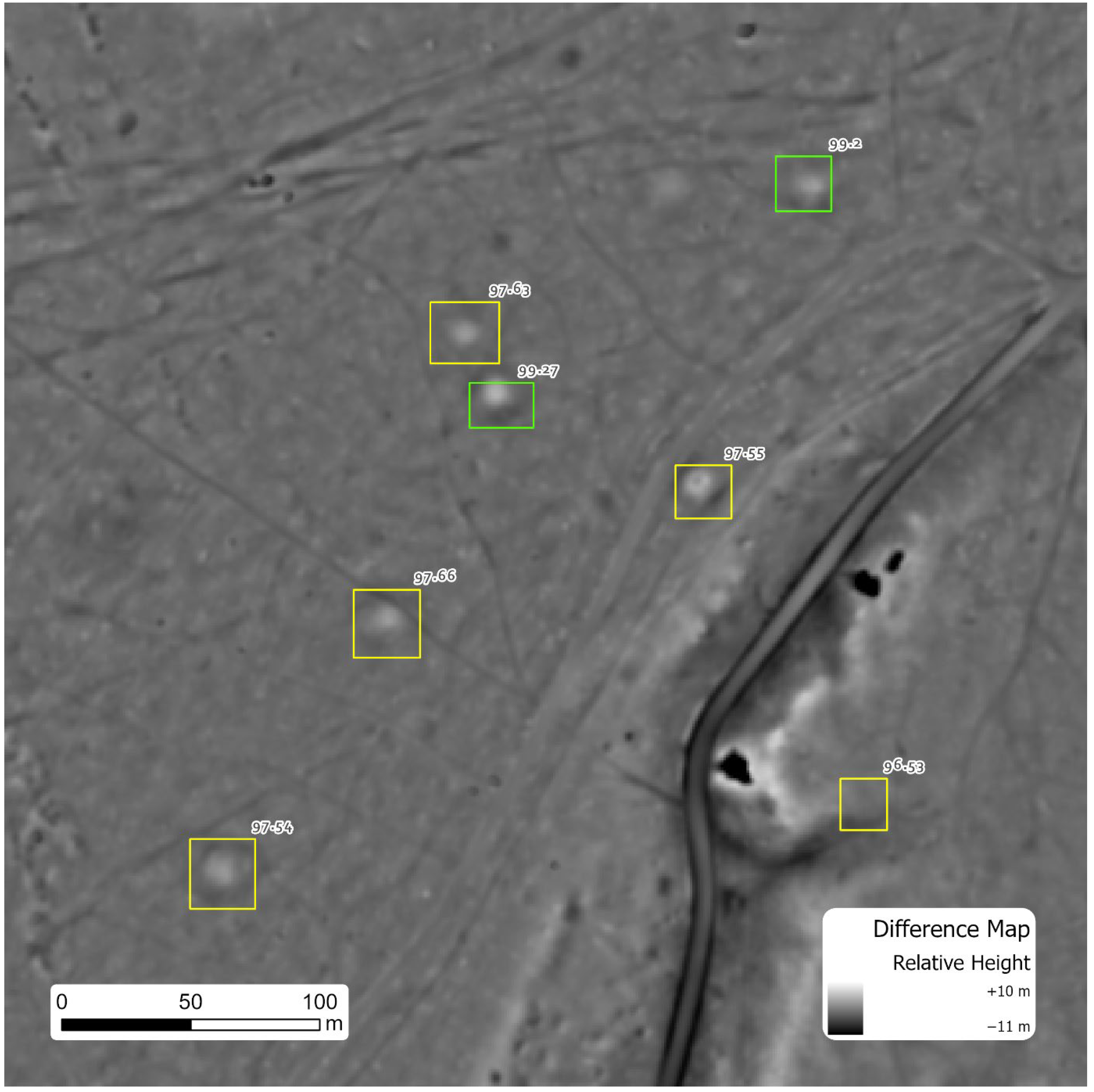
Figure 11.
Detected burial mounds in direct proximity to a hollow way (top). Green polygons represent true positives. Yellow polygons represent detections that were filtered out during post classification as their confidence was too low. Lowering the confidence threshold would have included them, however, too many false positives would have been included as well. Data source: [25].

Figure 12.
Detected mounds around each hollow way. The colors correspond to the zone, in which the mounds are located, and are also to be found in Table 1.
Figure 12.
Detected mounds around each hollow way. The colors correspond to the zone, in which the mounds are located, and are also to be found in Table 1.

Figure 13.
Accumulated area around all hollow ways (light blue) in dependency of the radius, compared to the additionally covered, ring-shaped area after increasing the radius (dark blue) and to the additionally detected mounds (yellow).
Figure 13.
Accumulated area around all hollow ways (light blue) in dependency of the radius, compared to the additionally covered, ring-shaped area after increasing the radius (dark blue) and to the additionally detected mounds (yellow).

Figure 14.
Maximum number of mounds of each hollow way in dependency on the radius.


Table 1.
Detailed list of all results. Numbers that are referenced in the text are highlighted.
| Remoteness (%) | Total Number of Detected Mounds | Mounds Per Zone | Zone of the Maximum Number of Mounds (x) | ||||||||||||||||
|---|---|---|---|---|---|---|---|---|---|---|---|---|---|---|---|---|---|---|---|
| No. | 500 m | 1000 m | 1500 m | 2000 m | 2500 m | 3000 m | 500 m | 1000 m | 1500 m | 2000 m | 2500 m | 3000 m | 500 m | 1000 m | 1500 m | 2000 m | 2500 m | 3000 m | |
| 1 | 98 | 3 | 12 | 13 | 15 | 15 | 15 | 3 | 9 | 1 | 2 | 0 | 0 | 🗶 | |||||
| 2 | 96 | 2 | 11 | 12 | 14 | 15 | 15 | 2 | 9 | 1 | 2 | 1 | 0 | 🗶 | |||||
| 3 | 95 | 0 | 0 | 1 | 1 | 5 | 20 | 0 | 0 | 1 | 0 | 4 | 15 | 🗶 | |||||
| 4 | 95 | 1 | 1 | 7 | 9 | 12 | 14 | 1 | 0 | 6 | 2 | 3 | 2 | 🗶 | |||||
| 5 | 94 | 0 | 0 | 0 | 0 | 0 | 0 | 0 | 0 | 0 | 0 | 0 | 0 | ||||||
| 6 | 94 | 0 | 2 | 8 | 15 | 15 | 15 | 0 | 2 | 6 | 7 | 0 | 0 | 🗶 | |||||
| 7 | 94 | 2 | 4 | 4 | 7 | 18 | 19 | 2 | 2 | 0 | 3 | 11 | 1 | 🗶 | |||||
| 8 | 94 | 0 | 0 | 1 | 1 | 1 | 2 | 0 | 0 | 1 | 0 | 0 | 1 | 🗶 | |||||
| 9 | 93 | 0 | 1 | 7 | 8 | 11 | 14 | 0 | 1 | 6 | 1 | 3 | 3 | 🗶 | |||||
| 10 | 93 | 0 | 0 | 0 | 0 | 0 | 0 | 0 | 0 | 0 | 0 | 0 | 0 | ||||||
| 11 | 93 | 0 | 1 | 2 | 2 | 3 | 6 | 0 | 1 | 1 | 0 | 1 | 3 | 🗶 | |||||
| 12 | 93 | 0 | 0 | 0 | 0 | 1 | 1 | 0 | 0 | 0 | 0 | 1 | 0 | 🗶 | |||||
| 13 | 93 | 1 | 1 | 7 | 10 | 12 | 13 | 1 | 0 | 6 | 3 | 2 | 1 | 🗶 | |||||
| 14 | 93 | 0 | 0 | 0 | 0 | 0 | 0 | 0 | 0 | 0 | 0 | 0 | 0 | ||||||
| 15 | 93 | 0 | 0 | 0 | 1 | 1 | 1 | 0 | 0 | 0 | 1 | 0 | 0 | 🗶 | |||||
| 16 | 93 | 0 | 1 | 1 | 1 | 2 | 3 | 0 | 1 | 0 | 0 | 1 | 1 | 🗶 | |||||
| 17 | 93 | 6 | 27 | 33 | 38 | 46 | 47 | 6 | 21 | 6 | 5 | 8 | 1 | 🗶 | |||||
| 18 | 93 | 0 | 0 | 0 | 0 | 3 | 4 | 0 | 0 | 0 | 0 | 3 | 1 | 🗶 | |||||
| 19 | 92 | 0 | 0 | 0 | 1 | 3 | 4 | 0 | 0 | 0 | 1 | 2 | 1 | 🗶 | |||||
| 20 | 92 | 0 | 3 | 7 | 10 | 13 | 14 | 0 | 3 | 4 | 3 | 3 | 1 | 🗶 | |||||
| 21 | 92 | 0 | 1 | 1 | 2 | 4 | 5 | 0 | 1 | 0 | 1 | 2 | 1 | 🗶 | |||||
| 22 | 92 | 0 | 0 | 3 | 9 | 12 | 14 | 0 | 0 | 3 | 6 | 3 | 2 | 🗶 | |||||
| 23 | 92 | 0 | 0 | 0 | 0 | 0 | 0 | 0 | 0 | 0 | 0 | 0 | 0 | ||||||
| 24 | 92 | 0 | 0 | 0 | 2 | 7 | 13 | 0 | 0 | 0 | 2 | 5 | 6 | 🗶 | |||||
| 25 | 92 | 1 | 1 | 1 | 1 | 3 | 3 | 1 | 0 | 0 | 0 | 2 | 0 | 🗶 | |||||
| 26 | 92 | 0 | 1 | 3 | 7 | 15 | 20 | 0 | 1 | 2 | 4 | 8 | 5 | 🗶 | |||||
| 27 | 91 | 0 | 0 | 0 | 0 | 3 | 4 | 0 | 0 | 0 | 0 | 3 | 1 | 🗶 | |||||
| 28 | 91 | 0 | 0 | 0 | 1 | 2 | 3 | 0 | 0 | 0 | 1 | 1 | 1 | 🗶 | |||||
| 29 | 91 | 0 | 0 | 6 | 10 | 14 | 20 | 0 | 0 | 6 | 4 | 4 | 6 | 🗶 | |||||
| 30 | 91 | 0 | 0 | 0 | 1 | 3 | 4 | 0 | 0 | 0 | 1 | 2 | 1 | 🗶 | |||||
| 31 | 91 | 0 | 1 | 1 | 3 | 3 | 3 | 0 | 1 | 0 | 2 | 0 | 0 | 🗶 | |||||
| 32 | 91 | 0 | 0 | 1 | 1 | 1 | 1 | 0 | 0 | 1 | 0 | 0 | 0 | 🗶 | |||||
| 33 | 91 | 0 | 1 | 2 | 2 | 3 | 4 | 0 | 1 | 1 | 0 | 1 | 1 | 🗶 | |||||
| 34 | 91 | 0 | 1 | 4 | 9 | 14 | 17 | 0 | 1 | 3 | 5 | 5 | 3 | 🗶 | |||||
| 35 | 91 | 1 | 1 | 1 | 1 | 3 | 3 | 1 | 0 | 0 | 0 | 2 | 0 | 🗶 | |||||
| 36 | 90 | 0 | 1 | 3 | 9 | 15 | 19 | 0 | 1 | 2 | 6 | 6 | 4 | 🗶 | |||||
| 37 | 90 | 1 | 1 | 2 | 6 | 8 | 8 | 1 | 0 | 1 | 4 | 2 | 0 | 🗶 | |||||
| 38 | 90 | 3 | 4 | 7 | 18 | 19 | 20 | 3 | 1 | 3 | 11 | 1 | 1 | 🗶 | |||||
| 39 | 90 | 1 | 2 | 2 | 4 | 9 | 18 | 1 | 1 | 0 | 2 | 5 | 9 | 🗶 | |||||
| 40 | 90 | 1 | 1 | 3 | 5 | 14 | 18 | 1 | 0 | 2 | 2 | 9 | 4 | 🗶 | |||||
| 41 | 90 | 1 | 1 | 3 | 5 | 14 | 18 | 1 | 0 | 2 | 2 | 9 | 4 | 🗶 | |||||
| 42 | 90 | 2 | 3 | 3 | 7 | 7 | 8 | 2 | 1 | 0 | 4 | 0 | 1 | 🗶 | |||||
| 43 | 90 | 0 | 1 | 4 | 7 | 8 | 8 | 0 | 1 | 3 | 3 | 1 | 0 | 🗶 | |||||
| Sum | 26 | 85 | 153 | 243 | 357 | 438 | 26 | 59 | 68 | 90 | 114 | 81 | 0 | 5 | 8 | 10 | 12 | 4 | |
| Mean | 0.6 | 2 | 3.6 | 5.7 | 8.3 | 10.2 | 0.6 | 1.4 | 1.6 | 2.1 | 2.7 | 1.9 | 0% | 13% | 21% | 26% | 31% | 10% | |
| % >0 | 33 | 60 | 72 | 84 | 91 | 91 | 33 | 44 | 53 | 65 | 74 | 65 | |||||||
Publisher’s Note: MDPI stays neutral with regard to jurisdictional claims in published maps and institutional affiliations. |
© 2022 by the authors. Licensee MDPI, Basel, Switzerland. This article is an open access article distributed under the terms and conditions of the Creative Commons Attribution (CC BY) license (https://creativecommons.org/licenses/by/4.0/).
Share and Cite
MDPI and ACS Style
Meyer-Heß, M.F.; Pfeffer, I.; Juergens, C. Application of Convolutional Neural Networks on Digital Terrain Models for Analyzing Spatial Relations in Archaeology. Remote Sens. 2022, 14, 2535. https://doi.org/10.3390/rs14112535
AMA Style
Meyer-Heß MF, Pfeffer I, Juergens C. Application of Convolutional Neural Networks on Digital Terrain Models for Analyzing Spatial Relations in Archaeology. Remote Sensing. 2022; 14(11):2535. https://doi.org/10.3390/rs14112535
Chicago/Turabian StyleMeyer-Heß, M. Fabian, Ingo Pfeffer, and Carsten Juergens. 2022. "Application of Convolutional Neural Networks on Digital Terrain Models for Analyzing Spatial Relations in Archaeology" Remote Sensing 14, no. 11: 2535. https://doi.org/10.3390/rs14112535
Note that from the first issue of 2016, this journal uses article numbers instead of page numbers. See further details here.