1. Introduction
Passive acoustic monitoring (PAM) sensors or microphones have been used for monitoring of soniferous species, discrimination among species, sexes, or age groups, and measurement of anthropogenic noise, as well as assessment of biodiversity [
1,
2,
3,
4]. Autonomous acoustic sensors are more cost-effective for large-scale, high-resolution wildlife surveys than human observers and their performance could meet or exceed that of human surveyors [
5,
6].
Non-synchronized passive acoustic sensor networks can detect the presence of a soniferous animal in a surrounding area but cannot locate it. Such information could be used for the assessment of different habitat usage but only across larger scales. The density of soniferous animals could be estimated by assessing a call rate—the average sound production rate for a species [
7]. In contrast, the localization of sound sources provides additional capabilities in the analysis of ecology and animal behavior—assessing individual animals’ positions or movements, localizing multiple individuals simultaneously to study their interactions, quantifying sound directionality, and inferring territory boundaries [
8]. In both cases, recording equipment should be widely available, affordable, and user-friendly to promote the uptake of passive acoustic sensors in the monitoring of wildlife.
Sugai et al. [
9,
10] reviewed the application of passive acoustic monitoring in the terrestrial environment and observed exponential growth in the number of published studies in the past decade. However, fully automated data analysis was applied only in 19% of the studies, of which one third involved bat signal studies due to existing software packages with built-in classifiers for automated recognition of bat species (e.g., Analook and Batsound). Analysis and handling of very large amounts of acoustic data are mentioned as a critical challenge in adopting PAM methodologies widely.
In this study, we are demonstrating a concept for automated detection and localization of red deer (Cervus elaphus) stags during the rut. A unique dataset of GPS time-synchronized acoustic records from a network of four sensors was collected and annotated to train and validate detection and localization algorithms. The accuracy threshold for red deer call detection was set to 90% to reach acceptable performance for the end-user. We are also demonstrating a novel automated approach for precise sound delay assessment which is the main challenge in the automation of sound source position estimation.
2. Related Work
Red deer (
Cervus elaphus) stags vocalize only during the rut (breeding season), to compete with other stags as well as to attract females. It has been reported that regular roaring in red deer advances ovulation and improves mating success [
11]. Several research groups [
12,
13,
14,
15] have studied vocal rutting activity in red deer and discussed the importance of using automated recording systems rather than human observers to provide full-scale data on the roaring activity. Enari et al. [
14,
15] have tested passive and active acoustic monitoring approaches for the assessment of sika deer (
Cervus nippon) populations in Japan during their rut period. They were able to detect deer males, even at sites with extremely low deer density where detection using existing methods based on spotlights and camera traps had failed. It was demonstrated that PAM could have a detection range of up to 140 m and a detection area of up to 6 ha in a defoliated forest, which is >100 times greater than that of camera traps. PAM also has higher deer detection sensitivity in comparison to camera traps. They concluded that the bioacoustic monitoring approach could be useful for the early detection of ungulate range expansion in the area. They used an approach based on hidden Markov models for clustering similar acoustic signals to build a reference dataset for the training of the supervised algorithm. They achieved recall rates of >0.70 for the detection of the half of call types. A similar approach based on hidden Markov models was previously used by Reby et al. [
16] for the detection and classification of red deer calls during the rut. They were able to achieve 93.5% accuracy in the detection of bouts of common roars.
Automated detection and classification of target sounds is a primary requirement for wider uptake of acoustic sensors in wildlife monitoring as it allows extracting the necessary information from audio records as well as it significantly reduces the time needed for data analysis. Rhinehart et al. [
8] observed that most papers surveyed did not classify species automatically, and those that did attempt automated species classification usually classified only a single species. Nevertheless, many studies show promising results in the automatization of target sound detection and classification.
Automatic processing of acoustic signals usually includes feature extraction, segmentation, classification frame-by-frame, and decision-making based on classification probability [
17]. Thresholding is the simplest method where detection occurs when the energy within a specified frequency band(s) exceeds a specified threshold—computationally inexpensive but often sensitive to nontarget background noise and signal overlap [
18]. Spectrogram cross-correlation is another method where detection occurs when the correlation coefficient against a template spectrogram exceeds a specified value—computationally inexpensive but relies on sufficiently representative template data [
19]. Hidden Markov models are used for detection and classification (probabilistically infers whether a signal of interest is present, based on an underlying multistate model)—incorporate temporal detail on signal/sequence but are complex for nonexperts to develop and require sufficient training/reference data [
15,
16]. Mac Aodha et al. [
20] used full-spectrum ultrasonic audio collected along road transects across Europe and labeled by citizen scientists from
www.batdetective.org (accessed on 16 May 2022) for the training of the convolutional neural network. Three main audio signal processing issues have been identified to advance acoustic monitoring—noise reduction, improved animal sound classification, and automated localization of sound sources [
8].
3. Methods
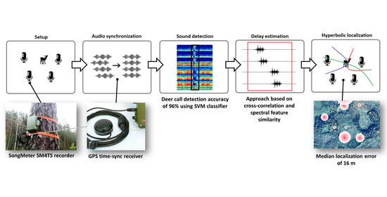
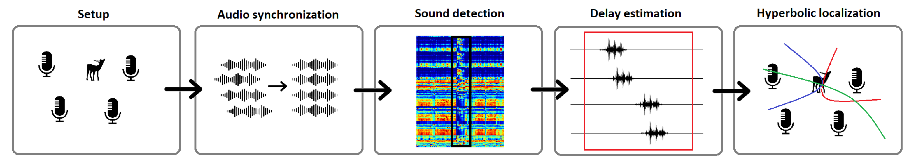
The development of automated acoustic wildlife data processing workflow requires an appropriate technological setup and pilot area for deer sound acquisition. Three main steps can be distinguished in the data processing workflow—deer sound detection, precise signal delay assessment between multiple microphones, and localization of the sound source (see
Figure 1). Finding the target sound in all recorders and precise calculation of the delay is the main challenge in this workflow. In addition, factors such as wind speed and direction and the environment itself can shift the measured delay between the recorders of an audio source. Noise reduction is not distinguished as a separate step; instead, it is a part of data preprocessing in the sound detection step.
Description of the workflow used in this study:
Setup—recorder deployment in the area of interest and data gathering during the deer rutting period.
Audio synchronization—synchronization of multiple microphone clocks using GPS time-sync receiver and filtration of only synchronized audio record for deer call localization.
Sound detection—application of the best-performing binary classifier for deer call detection. The classifier has been trained on various deer vocalizations and environment sounds and is used to find audio timestamps where deer calls are heard in all recorders in a given time window.
Delay estimation—precise assessment of deer call starts in synchronized audio signals from multiple microphones and calculation of acoustic signal arrival delays. This step is applied only for deer calls detected in all four microphones. The reference signal is selected as the signal where deer sounds were detected first; afterwards, this signal is used to find a signal delay in the other three recorders. Signal delay can be calculated using cross-correlation or the proposed spectral similarity methods.
Hyperbolic localization—geospatial localization of signal source from obtained signal delay values and recorder locations.
3.1. Pilot Area
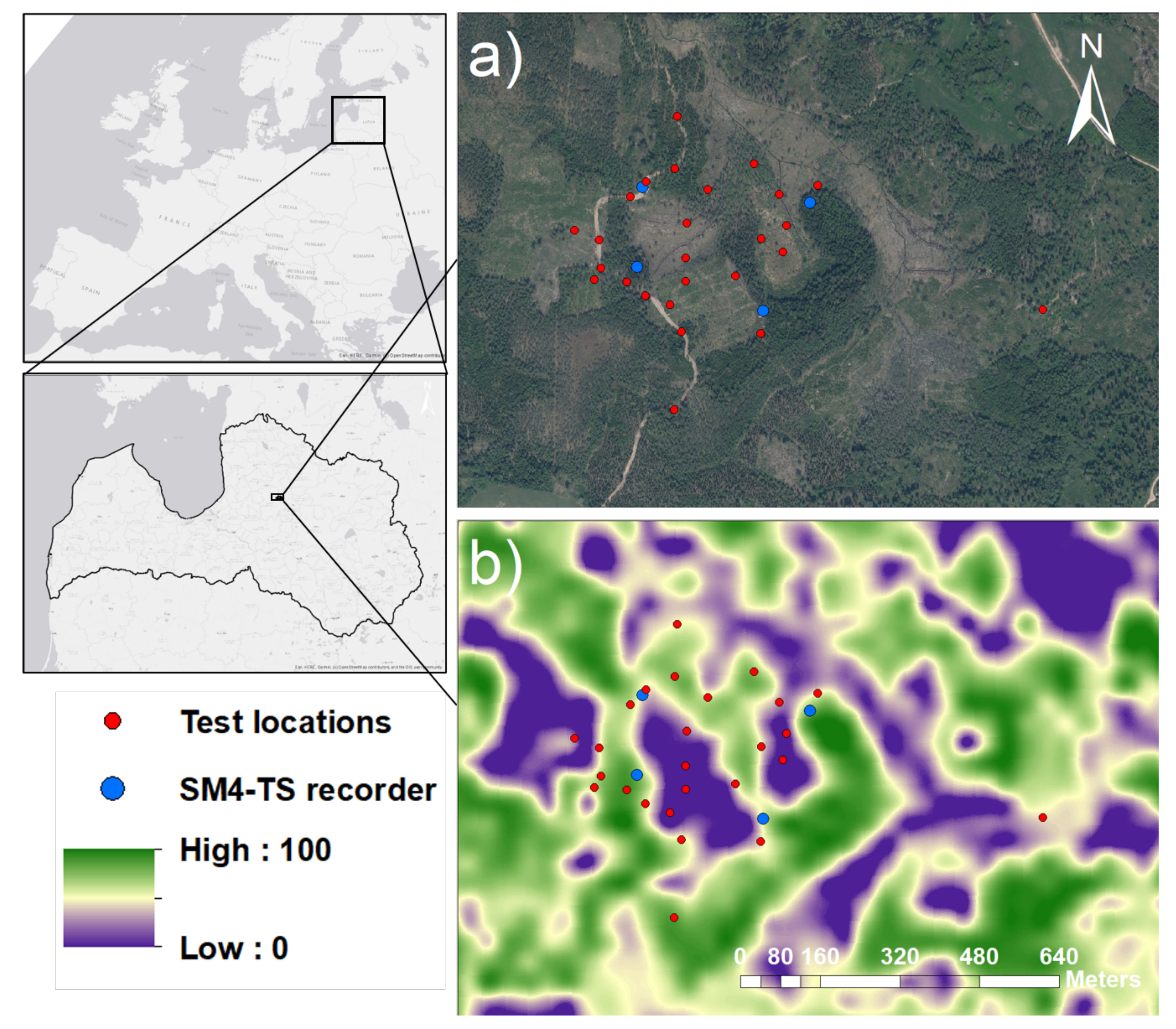
The pilot area is located in Latvia, near Rāmuļi, at latitude 57.186, longitude 25.486, 10 km from the border of Gauja National Park, the largest national park in Latvia (see
Figure 2) [
21]. The territory around the pilot area consists of mostly forests, coppices, and marshlands. The dominant tree species in the territory are
Picea abies and
Betula pendula. The area has minor hills. A drainage ditch and a dirt road is going through the area. The territory is private and experiences a moderate amount of anthropogenic disturbances such as forestry and hunting, and the closest active road is 800 m from the location. According to the official data from the State Forest Service, the density of red deer in the pilot area is 35 animals per 1000 ha of forest area in 2021.
3.2. Deer Sound Acquisition
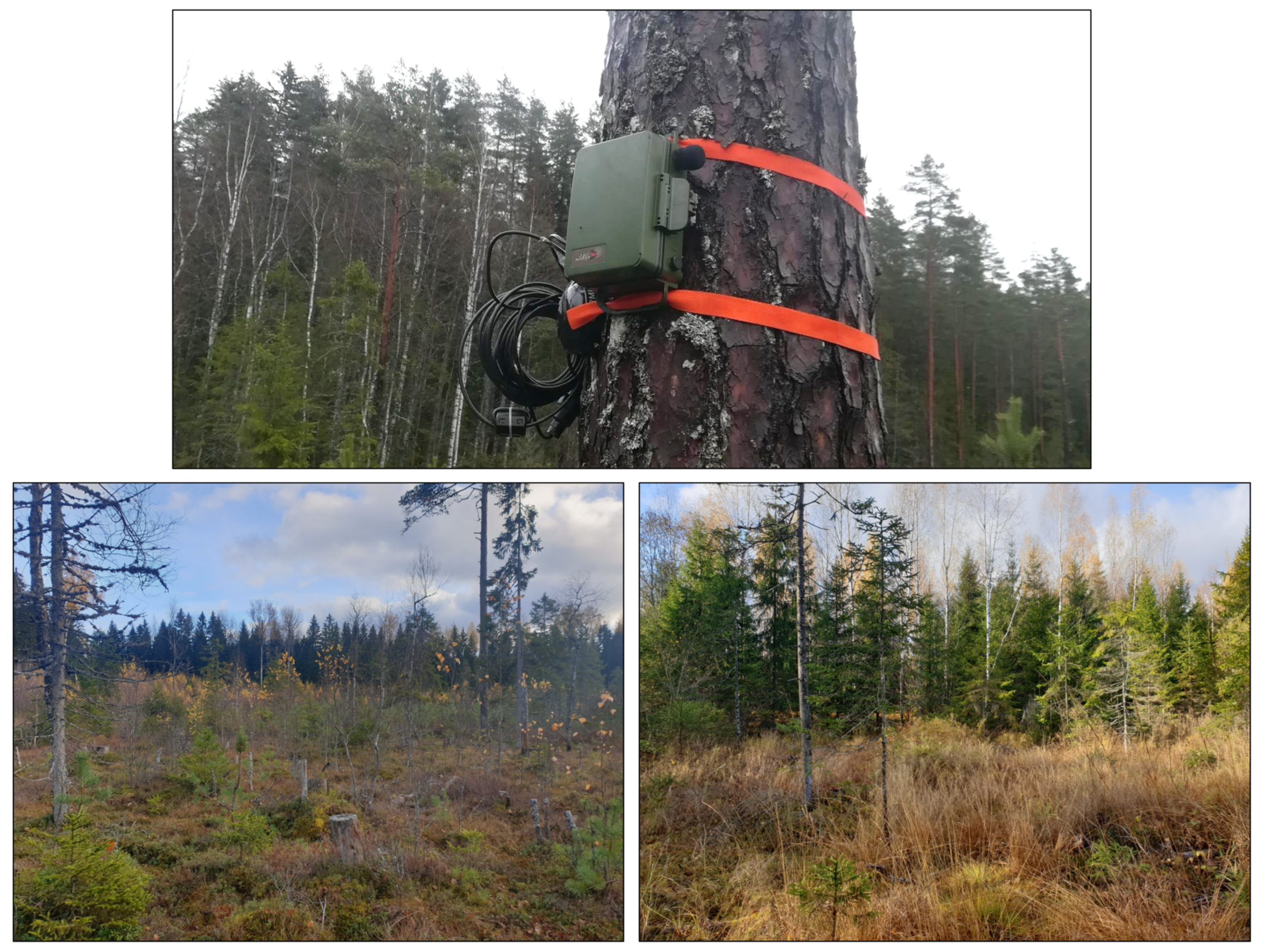
The sound acquisition was performed using the Song Meter SM4TS which is specially designed to help scientists triangulate the location of vocalizing animals. The SM4TS (
Figure 3) is a modified SM4 recorder that utilizes a GPS time-sync receiver to synchronize the clocks on multiple recorders within one millisecond. The recordings were made with a sample rate of 8 kHz. The two built-in omnidirectional microphones have the following characteristics: sensitivity—−35 ± 4 dB (0 dB = 1 V/pa@1 kHz), signal to noise ratio −80 dB at 1 kHz, and max input sound level −126 dB. Recorded audio data were stored in uncompressed form. Data acquisition was performed from 30 August until 27 September 2021, and recorders were scheduled to automatically turn on at 7:00 p.m. and turn off at 7:00 a.m., with a file length of 1 h. High-capacity SD cards (256 GB SanDisk Extreme Pro SDXC) were used for data storage to ensure continuous data collection throughout the rutting period.
Recorders were placed in a rectangular formation with a distance ranging from 160 m to 370 m (
Figure 2) and were mounted on hillsides and tree trunks at 4–7 m height facing the middle of the grid to minimize sound-wave obstruction by vegetation and terrain and increase the chances of the same sound source being detected by all units. The recorders were visited every week to ensure that they were operational and change batteries if needed.
Precise time synchronization is essential for sound source localization applications; therefore, a commercially available of-the-shelf solution was chosen for this study. However, it was noted that GPS time synchronization tends to break, resulting in 20…25% of data loss for localization assessment. The success or failure of synchronization can be determined from record metadata. Non-synchronized data was not used for localization tests but still was a valuable source for building of deer call database.
The measured location by SM4TS GPS receivers oscillates over time; therefore, the average of several days’ measurements of longitude and latitude were chosen as the true recorder location. Another option would be to measure the receiver coordinates using a more precise GPS receiver.
3.3. Deer Sound Detection
The deer calls have to be identified within the recording to enable audio delay calculation. The process of identifying sounds can be carried out using various approaches, starting from manual labeling to fully automated. As the gathered data contains hundreds of hours of recordings, an automated approach was chosen to identify deer sounds.
To make sure that all audio files have a consistent loudness and format, the audio files underwent the following procedure:
Loudness normalization in accordance with EBU R 128 Standard.
Stereo to mono conversion.
Wind noise reduction using 150 Hz high-pass filter.
3.3.1. Semiautomatic Approach for Dataset Creation
Initially, a manual dataset of deer and background sounds was created, each class containing 20 samples, which consisted of different types of deer calls identified in the recordings. Afterwards, a semiautomatic approach was used to find similar sounds in available audio files. To expand the dataset, firstly, we chose a sample from the small dataset and the 1 h long recordings. The feature similarity between the reference and the examined audio was measured with peak signal-to-noise ratio (PSNR); afterwards, the data were sorted according to the error score and the top 50 closest matches were saved as 2 s audio clips. As a next step, these extracted audio clips were inspected manually to remove outliers and separated into two classes—”deer calls” and “not deer calls”. The class “deer calls” consisted of various types of deer vocalizations such as long and short common roars, chase barks, and grunts. Class “not deer calls” consisted of various nature sounds: wind, rain, and sounds from other animals. The outliers were sounds that the expert could not assign to any of the classes with sufficient confidence and were not included in the reference dataset. With the semiautomatic approach, the reference dataset was expanded to 800 samples per class. The spectral features, which are a popular choice in many audio recognition applications, were calculated for 0.5 s samples with a step of 0.01 s, were as follows:
Linear spectrum (feature count: 2000).
Mel spectrum (no. of bandpass filters in filterbank: 32).
Bark spectrum (no. of bandpass filters in filterbank: 32).
Equivalent rectangular bandwidth (ERB) (no. of ERB bands: 28).
The pseudocode described in Algorithm 1 shows the procedure for similarity search based on spectral features. Each row in
and
holds one sample, and columns correspond to individual features. To reduce noise, the extracted features were averaged using the moving mean with the step 5. Function
featureSetep2sampleTime() is used to correctly map timestamps for each sample in
. The feature similarity between reference audio and segments of the same length from test audio is carried out using PSNR.
| Algorithm 1 Spectral similarity search. |
| 1: Fs = 8000 Hz |
| 2: windowSize = 5 |
| 3: Aref—audio reference file |
| 4: Atest—audio test file |
| 5: Arefn ← gainNormalization(Aref) |
| 6: Atestn ← gainNormalization(Atest) |
| 7: Areff ← audioFeatureExtractor(Arefn) |
| 8: Atestf ← audioFeatureExtractor(Atestn) |
| 9: Areffm ← moveMean(Areff, windowSize, rows) |
| 10: Atestfm ← moveMean(Atestf, windowSize, rows) |
| 11: score = zeros(size(Atestfm,rows) − size(Areffm,rows)) |
| 12: for i = 1,2,…,size(score) do |
| 13: score(i) = psnr(Areffm, Atestfm(i:i + size(Areffm) :)) |
| 14: end for |
| 15: scoreSorted, scoreSortedIdx = sortAscend(score) |
| 16: audioIdx = featureSetep2sampleTime(scoreSortedIdx) |
| 17: for i = 1, 2,…,50 do |
| 18: saveAudio = Atest(audioIdx(i):audioIdx(i) + 2Fs) |
| 19: end for |
3.3.2. Automatic Approach for Deer Sound Detection
After creating the dataset of audio files, several classifiers were trained based on spectral features calculated for 0.5 s samples with a step of 0.25 s, which were as follows:
Mel spectrum (no. of bandpass filters in filterbank: 32).
Bark spectrum (no. of bandpass filters in filterbank: 32).
Equivalent rectangular bandwidth (ERB) (no. of ERB bands: 28).
Mel frequency cepstral coefficients (MFCC) (no. of coefficients for window: 13).
Gammatone cepstral coefficients (GTCC) (no. of coefficients for window: 13).
Spectral centroid.
Spectral crest.
Spectral decrease.
Spectral entropy.
Spectral flatness.
Spectral kurtosis.
Spectral roll off point.
Spectral skewness.
Spectral slope.
Spectral spread.
Harmonic ratio.
The process for preparing features is similar to the similarity search. In Algorithm 2, features are prepared in two steps: first, all the spectral features are extracted from the 0.5 audio segments, and afterwards, the features are averaged using the moving mean.
| Algorithm 2 Feature extraction. |
| 1: Fs = 8000 Hz |
| 2: windowSize = 5 |
| 3: Asample−audio file |
| 4: AsampleNorm ← gainNormalization(Asample) |
| 5: sampleRange = 1:Fs/4:len(AsampleNorm)−Fs/2 |
| 6: fvecList = [] |
| 7: for i = sampleRange do |
| 8: Atmp ← AsampleNorm(i:i + Fs/2) |
| 9: Afvec ← audioFeatureExtractor(Atmp) |
| 10: Astd = std(Atmp) |
| 11: Apv = Astd/ |
| 12: fvecList(i) = [AfvecAstdApv] |
| 13: end for |
| 14: fvecListConcat = [] |
| 15: for i = 3,4,…,size(fvec, List, rows)−2 do |
| 16: ftmp = fvecList(i − 2:i + 2, :) |
| 17: fmean = mean(ftmp, rows) |
| 18: fstd = std(ftmp, rows) |
| 19: fpv = fstd/ |
| 20: fvecListConcat(k,:) = [fmean fstd fpv] |
| 21: end for |
| 22: fvecListMean ← moveMean(f vecListConcat, windowSize, rows) |
Five machine learning models were tested on a dataset that only included nature sounds, such as deer vocalizations, dog barking, birds chirping, rain, and wind sounds. The chosen models for deer sound classification were support vector machine, linear discriminant analysis, decision tree, k-nearest neighbors, and long short-term memory algorithms, and the best-performing one was chosen for further implementation in the workflow.
3.3.3. Support Vector Machine (SVM)
Support vector machine analyzes input data and recognizes patterns in a multi-dimensional feature space called the hyperplane. An SVM model represents data as points in space, mapped so that the samples of the separate categories are clearly separable. New samples are then mapped into that same space and predicted to belong to a category based on the previously established hyperplanes [
22]. The reported linear kernel SVM used weighted standardizing where the software centers and scales each predictor variable by the corresponding weighted column mean and standard deviation. Matlab function
fitcsvm() was used with parameters KernelFunction-linear and Standardize-true.
3.3.4. Linear Discriminant Analysis (LDA)
Discriminant analysis is a classification method that assumes that class features have different Gaussian distributions. To train a classifier, the fitting function estimates the parameters of a Gaussian distribution for each class in such a way as to minimize the variance and maximize the distance between the means of the two classes. To predict a class, the data are projected into LDA feature space and the trained model finds the class with the smallest misclassification cost [
23]. Matlab function
fitcdiscr() was used, and to avoid computations errors with low feature count, the DiscrimType was set to pseudoLinear which means that all classes have the same covariance matrix and the software inverts the covariance matrix using the pseudo inverse.
3.3.5. K-Nearest Neighbors Algorithm (kNN)
K-nearest neighbors algorithm uses feature similarity to predict the values of new samples based on how similar they match the points in the training set. The similarity is usually measured as a distance between points, where the Euclidean distance is one of the most popular choices [
24]. The presented results are with the model created by Matlab function
fitcknn() where the nearest neighbor count was set to 5.
3.3.6. Decision Tree (DT)
Decision trees classify instances by sorting them down the tree from the root to some leaf node, which provides the classification of the instance. An instance is classified by starting at the root node of the tree, testing the attribute specified by this node, then moving down the tree branch corresponding to the value of the attribute [
25]. Matlab function
fitctree() was used with the default parameters.
3.3.7. Long Short-Term Memory (LSTM)
Long short-term memory networks are a variant of recurrent neural networks capable of learning long-term dependencies. They were introduced by Hochreiter and Schmidhuber [
26]. The LSTM network was implemented in Matlab with the fallowing structure: sequenceInputLayer, lstmLayer = 200, fullyConnectedLayer, softmaxLayer, and classificationLayer. The number of epochs was set to 30 and the minimum batch size to 64.
3.4. Audio Delay Calculation
The audio delay calculation is a challenging task because the recorded deer vocalizations are affected by such factors as different background noise for each of the recorders and possible shifts in the audio spectrum due to the influence of wind and the environment. To eliminate some of the noise, signals used in audio delay calculation were filtered using 150 Hz high-pass filter.
Based on SM4TS audio recorder synchronization information in audio file names consisting of recording date (YYYYMMDD), synchronization symbol
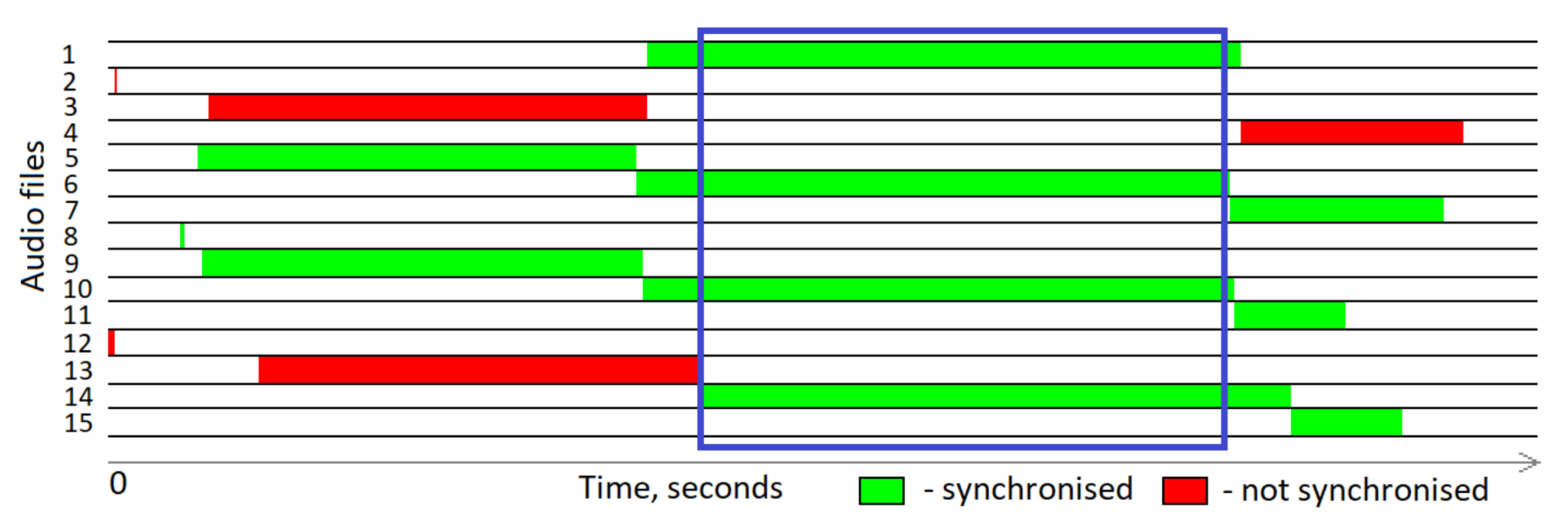
$ and time (HHMMSS), Matlab script was created to find time periods where all recorders are synchronized.
Figure 4 shows recorded files as green and red rectangles, where the left end shows the start of an audio file and the right side shows the end. The start of a new file is guaranteed to be with second precision, this means that filename with string ‘000001’ started exactly at 00:00:01.000 ± 0.001 s.
Afterwards, the synchronized audio files were scanned for deer vocalizations using the trained classification model. Initially, the search window is set to 0.25 s to save computation time. Once a potential location of deer vocalization is found, a more thorough search is performed in ±0.25 s range with a step of 0.01 s. Afterwards, a reference point is defined where classification switches from background to deer vocalization. The window for signal offset search is set to ±2 s from the detected location; due to the physical placement of SM4TS recorders, the offset signals should be present within the search window. To proceed with localization, deer call should be detected in all recorders within the specified time window.
3.4.1. Manual Detection
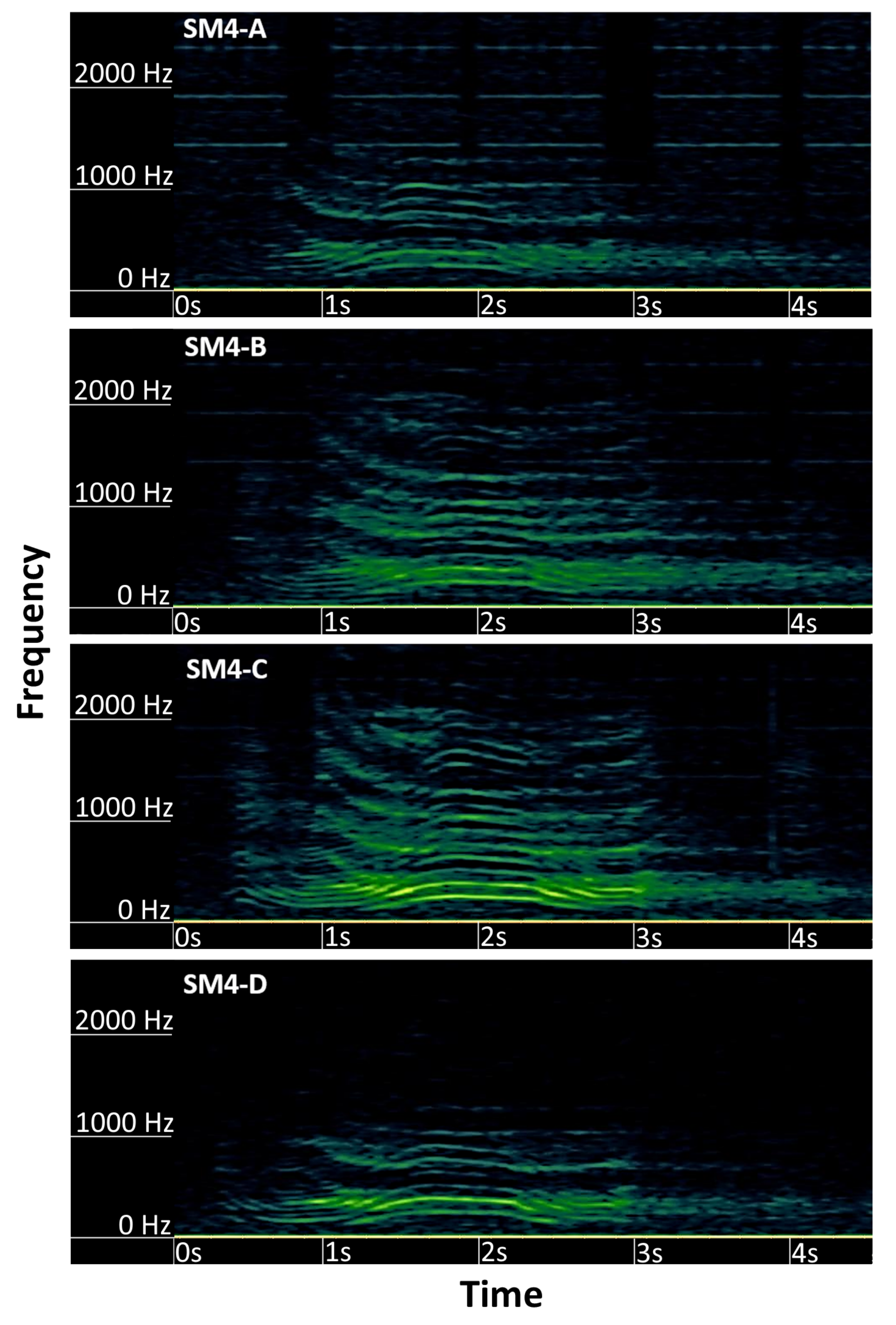
Sound delays were manually measured to create reference data with visual spectrogram analysis in the Kaleidescope software version 5.4.6. We searched for deer calls that were audible in all four recorders (see
Figure 5) and looked for the features in their spectrogram that could be identified and matched, and noted the exact timestamp of the feature for each recorder. Only deer calls that had visually distinguished features in all four recorders were used.
3.4.2. Cross-Correlation
Once a search location is known, a reference window of ±0.5 s is selected and cross-correlation is used to find the same signal in other recorders. This method works well when the signals are clearly audible, but becomes imprecise when noise is present in the signals.
3.4.3. Spectral Similarity
Besides searching signal correlation in the time domain, it also can be estimated in the frequency domain using spectrograms. In this article this is referred to as spectral similarity and it was measured by calculating spectral features and measuring their similarity with other signals. To obtain a more accurate delay measure, the window length was set to 1 s and a step of 1 millisecond which matches the accuracy provided by the GPS synchronization. The extracted spectral features were the same ones used in the
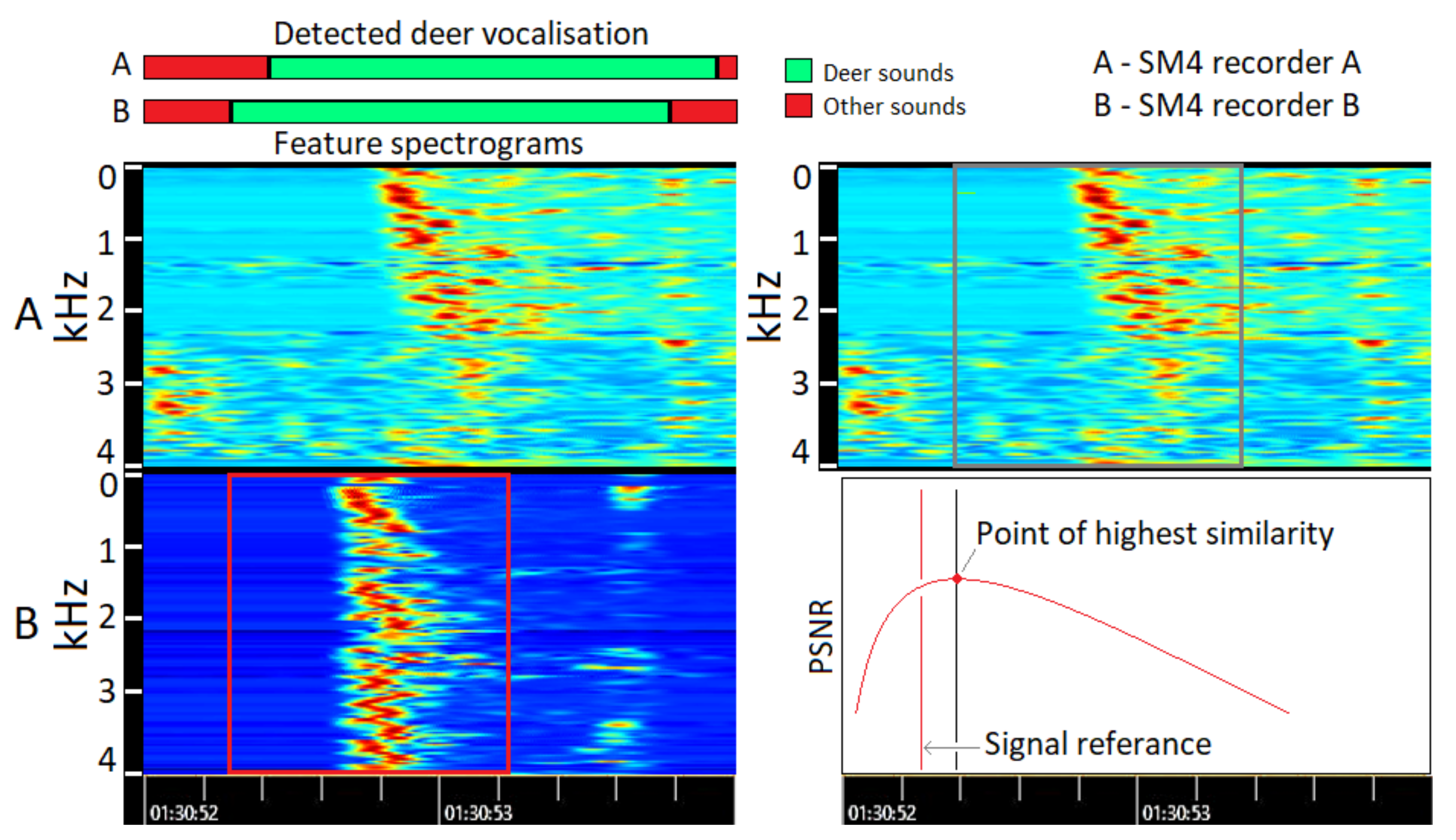
spectral similarity search. The spectrogram was normalized and raised to a power of 0.2, also known as gamma correction, to bring out more details. All the spectral similarity measurements were performed using peak signal-to-noise ratio (PSNR). Other methods, such as root mean square error (RMSE), structural similarity index (SSIM), feature-based similarity index (FSIM), information theoretic-based statistic similarity measure (ISSM), and 2D cross-correlation, were tested; nevertheless, PSNR gave the most precise results. An example of delay estimation using two recorders is shown in
Figure 6. The similarity search is executed because deer vocalizations are detected in both audio files according to the binary classifier. The reference signal is chosen to be recorder B (red square) because, in the detected signal region, signal B was detected first and had higher signal power than signal A. Afterwards, the red square is compared to spectral features in recorder A as a sliding window and the PSNR value is calculated for each step.
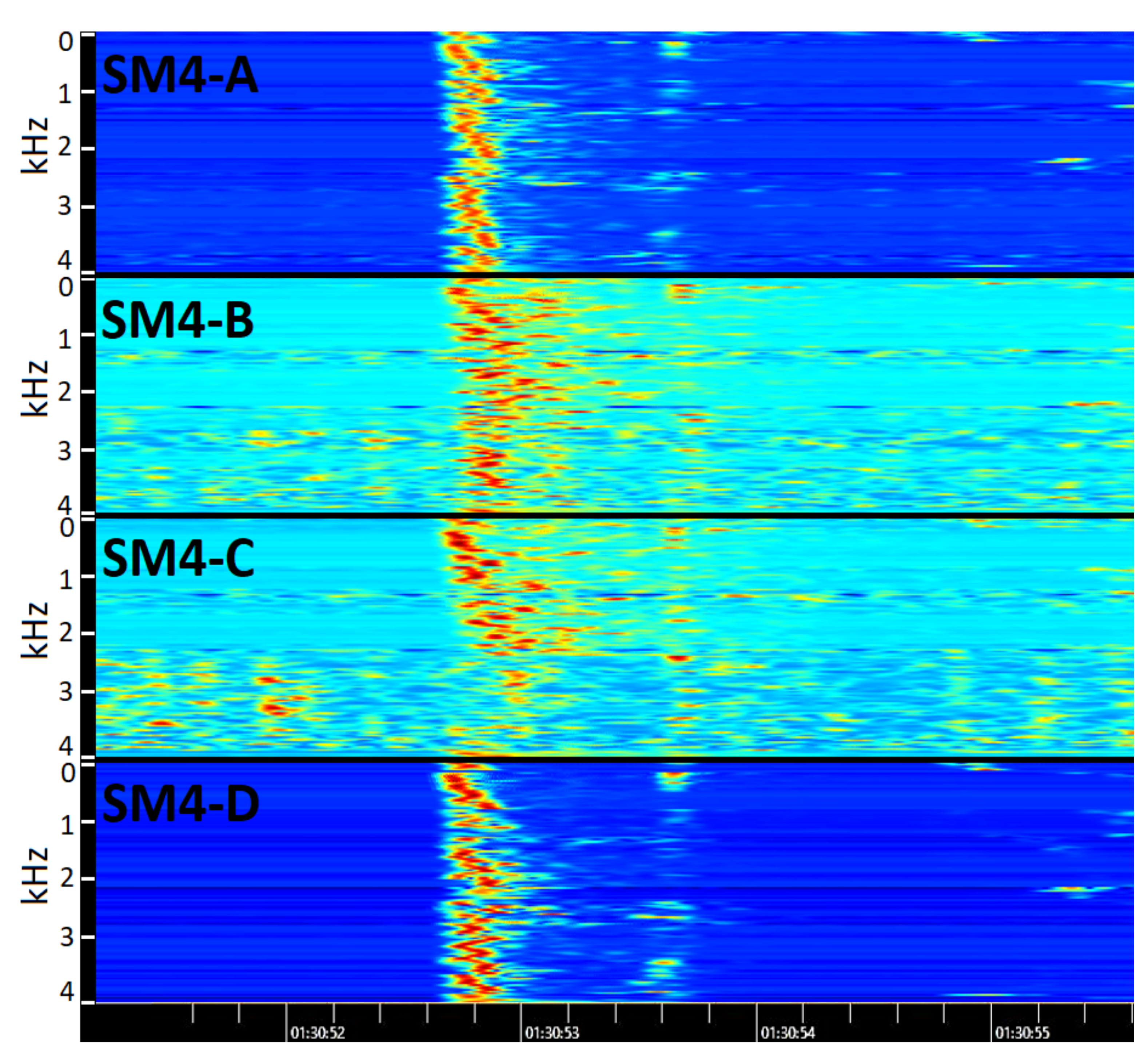
The correctness of the estimated signal delays can be shown visually by shifting signals according to the calculated delay in relation to the reference signal. An example is shown in
Figure 7, where the spectrograms from recorders A, B, and C are shifted to match the reference signal D.
3.4.4. Audio Delay Estimation—Spectral Selected
To improve the spectral similarity search, some of the spectral features, which do not contain relevant information, can be discarded. This action removes irrelevant features from the spectrogram and as a consequence improves the correctness of the PSNR score. Essentially, the aim of this approach is to find features that retain their pattern, even if the signal is degraded. Once the features are selected, the signal delay was found based on feature similarity according to PSNR. The feature selection procedure is as follows:
Select a reference signal.
Extract spectral features of the reference signal.
Generate white Gaussian noise with SNR of 30 dB.
Add white Gaussian noise to the reference signal.
Extract spectral features from the noise added signal.
Perform cross-correlation between reference and noise added signal for each spectral feature individually.
Select features with the highest correlation coefficient at the expected time delay.
The reference signal is selected automatically: firstly, deer vocalizations are found using the classifier; if deer vocalizations are present in all four recorders, a time frame is selected for further investigation; afterwards, the reference signal is chosen as the signal segment which has the highest signal power.
3.4.5. Audio Delay Estimation—Spectral 2 Stage
The delayed signal spectrogram patterns can look very different; usually, the signal with the largest delay has a fading pattern when compared to the first signal which is used as zero references. To address this problem, an additional similarity search was calculated for a grid-like structure, where the spectrum is divided into a 2D grid of 5 × 5 cells and PSNR is calculated individually for each grid cell. The total PSNR score is the sum of all grid cell scores, divided by the standard deviation of the corresponding cell. Algorithm 3 shows the score calculation between a reference and one step in the search for a similar signal in other recorders. Actions from line 10 and further have to be repeated for each 1 ms step in the
signal. When all the scores are calculated, the delay value is chosen to be the time indicated by maximum score value as shown in the PSNR plot in
Figure 6.
| Algorithm 3 Similarity score calculation in Spectral 2 stage approach. |
| 1: Sref−reference spectrogram |
| 2: Cref ← spectrogram2blocks(Sref, 5, 5) |
| 3: Wref = (5, 5) |
| 4: for i = 1, 2,…, 5 do |
| 5: for j = 1, 2,…, 5 do |
| 6: Wref (i, j) = std(Cref (i, j)) |
| 7: end for |
| 8: end for |
| 9: Wrefnorm = Wref/∑ Wref |
| 10: Stest−test spectrogram |
| 11: Ctest ← spectrogram2blocks(Stest, 5, 5) |
| 12: score = 0 |
| 13: for i = 1, 2,…, 5 do |
| 14: for j = 1, 2,…, 5 do |
| 15: score + = PSNR(Ctest (i, j), Cref (i, j) ∗ Wrefnorm (i, j)) |
| 7: end for |
| 8: end for |
3.5. Hyperbolic Localization
According to J.L. Spiesbergera [
27], for hyperbolic localization in two spatial dimensions, as a minimum, four recorders must be used. J.L. Spiesbergera also demonstrated that localization only using three recorders can have up to 100 m errors and that in some cases, the solutions will be ambiguous. The hyperbolic calculation was performed according to the approach by Watkins and Schevill [
28] as described in [
27]. For implementing the hyperbolic triangulation, geographic coordinates were converted to a local, Cartesian coordinate frame; therefore, latitude and longitude coordinates were converted to x and y coordinates according to Chirs Murphy’s paper [
29]. The arrays
lat contain four latitude coordinates and array
lon contain four longitude coordinates. The conversion from degrees
(lat/lon) to meters was performed as follows:
where
and
are an arbitrary latitude and longitude origin which is equivalent to
,
. The distances between recorders
r were calculated according to Euclidean distance between two points.
The speed of sound is defined as a constant,
c. The distance between the
ith receiver at
and a source at
s is
so we have
. Placing the first receiver at the origin of the coordinate system, one subtracts the equation for
from
to obtain
, which simplifies to
where the four receivers
and
is the inverse of
R. The Cartesian coordinates of receiver
i and the source are
and
. Use
in the square of Equation (
1) to solve for
to obtain
where
,
and
.
The described solution was implemented in Matlab, the inputs to the algorithm are the four audio signal delay values and distances between the recorders, where the first detected signal has a delay value of 0 and the recorder which contains this signal is used as the origin point to measure the distance to other recorders. The delay values can be found by cross-correlation or spectral similarity.
3.6. Controlled Tests
To test the accuracy of the hyperbolic localization and compare manual and automatic sound delay calculation approaches, controlled tests were performed in the study area on 19 October 2021 (see
Figure 2). The SM4TS unit recording length was set to 1 min length to minimize the chance of an error with synchronization to the GPS clock and ruining test results. Sounds were created in 26 different locations in the study area, and the position and time of the sound source were recorded. Locations were noted only after standing still for a duration of time and confirming a good connection to the GPS satellites to reduce GPS error. Out of the 26 test sounds, 9 were located within the grid covered by the 4 recorders, and 17 were located outside, with the furthest test sound being 250 m from the perimeter of the grid and 800 m away from the furthest recorder. All test sounds were audible in all recorders. Automatic hyperbolic localization was not possible on 11 of the test sounds, because they were split between two files in at least one of the recorders. The regions of interest in the sound samples were identified manually.
4. Results
The performance of deer sound detection and localization was tested using annotated datasets. In the case of sound detection, the available dataset was split into training and validation subsets where deer calls were manually annotated by an expert. In the case of sound localization, there was no information on soniferous deer locations; therefore, controlled tests were used to test the accuracy of sound source localization.
4.1. Deer Sound Detection Results
The performance of different detection algorithms is shown in
Table 1. The algorithms were evaluated using 5-fold cross-validation and the same dataset structure was used to test all five classifiers. The linear SVM model demonstrated the best performance—96.46% followed by LDA with 95.67% and kNN with 95.52%. In all of the cases, obtained accuracy was >90% which was set as a criteria by the end-user. The best-performing SVM model was chosen for implementation in the automated data processing workflow.
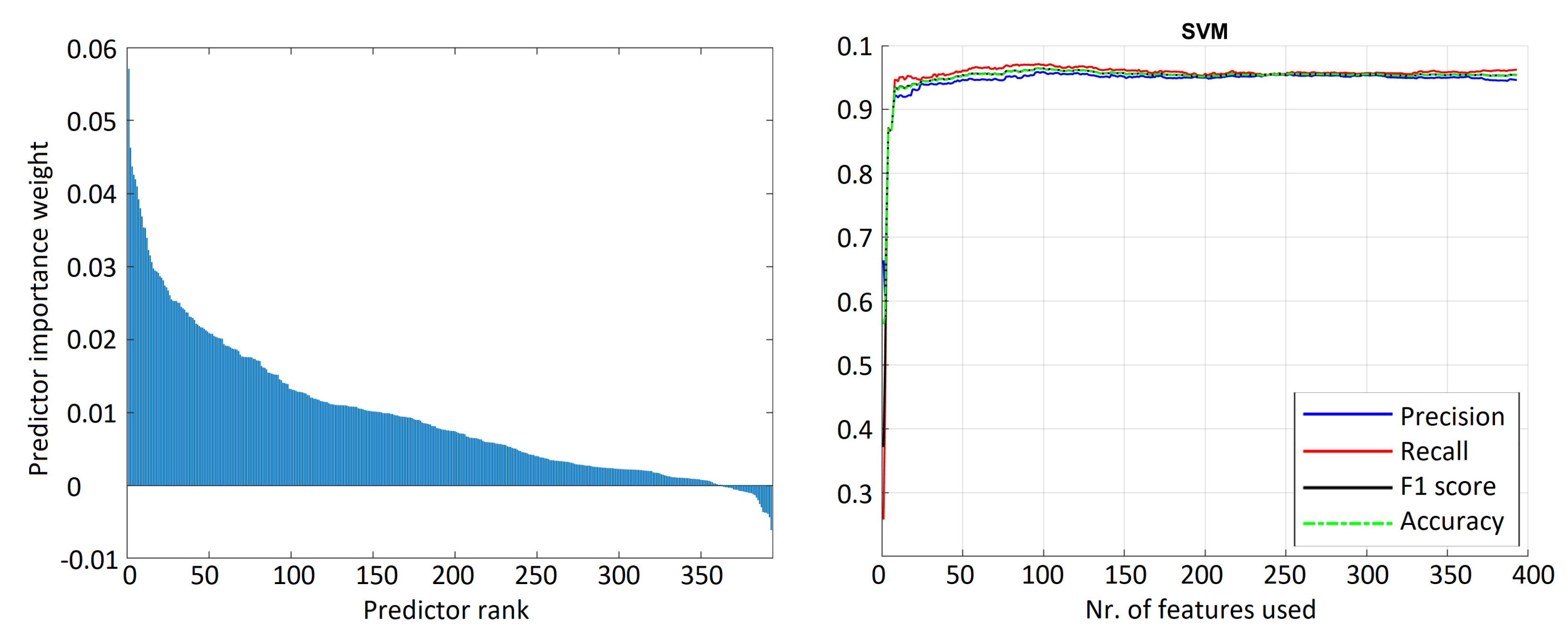
To avoid overfitting issues, ReliefF [
30] feature ranking algorithm was used. The final model used in classification was trained with features that provided the highest accuracy value. Model results using feature selection are shown in
Figure 8 and
Figure 9. An accuracy threshold of 90% could be achieved by using 20 of the most significant features. Even though the accuracy is very high using all features, the accuracy curve flattens after using only 150 features out of 393; in addition, the model gave a signification amount of false positives. After using only features with positive rank, the SVM model had fewer false positive cases.
Noise filtering (150 Hz high-pass filter) was applied to noisy data. It was observed that the inclusion of features from filtered audio had a 3% increase in overall model accuracy for all the tested models. Therefore, such a relatively simple noise filter was introduced into the workflow.
4.2. Sound Localization Results
Precise assessment of sound delay between different microphones is crucial for deer sound localization. Soniferous deer locations were unknown; therefore, we used controlled sound tests for evaluation of different sound delay assessment approaches, including manual sound delay calculation performed by a human expert. Therefore, to test the accuracy of the hyperbolic localization and compare manual and automatic sound delay calculation approaches, controlled tests were performed in the study area on 19 October 2021 (see
Figure 2). The SM4TS unit recording length was set to a 1 min length to minimize the chance of an error with synchronization to the GPS clock and ruining test results. Sounds were created in 26 different locations in the study area, and the position and time of the sound source were recorded. Locations were noted only after standing still for a duration of time and confirming a good connection to the GPS satellites to reduce GPS error. Out of the 26 test sounds, 9 were located within the grid covered by the 4 recorders, and 17 were located outside, with the furthest test sound being 250 m from the perimeter of the grid and 800 m away from the furthest recorder. All test sounds were audible in all recorders. Automatic hyperbolic localization was not possible on 11 of the test sounds, because they were split between two files in at least one of the recorders. The regions of interest in the sound samples were identified manually.
The performance of the manual approach and four automated approaches is shown in
Table 2. The error represents the distance between the GPS measured location (reference) and the location calculated according to hyperbolic localization using different signal time delay assessment approaches. In the case of manually obtained sound delays by a human expert, the median error was 43 m with a standard deviation of 63 m. In all cases of automated delay assessment, the median error was smaller in comparison to the manual approach, demonstrating the potential of automated approaches to increase the accuracy of sound localization. The human expert indicated that sound delay assessment is a challenging task and there is a high risk of error. Signal cross-correlations and spectral feature similarity can be considered as baseline methods in automated sound analysis. The cross-correlation-based approach demonstrated a slightly improved median error of 39 m in comparison to the manual approach but the standard deviation was much higher—240 m. It tended to fail in separate cases resulting in extremely high errors >200 m. The spectral feature similarity approach demonstrated more stable performance (standard deviation of 56 m) with a slightly lower error—37 m. In comparison, two modified methods (
Spectral selected and
Spectral 2 stage) show significant improvement both in localization accuracy as well as error consistency.
Spectral selected approach resulted in the median error of 27 m with standard deviation of 59 m but
Spectral 2 stage approach showed the best performance with a median error of 16 m and a standard deviation of 38 m. Therefore, the automated sound delay assessment approach based on
Spectral 2 stage detector was further implemented in the workflow.
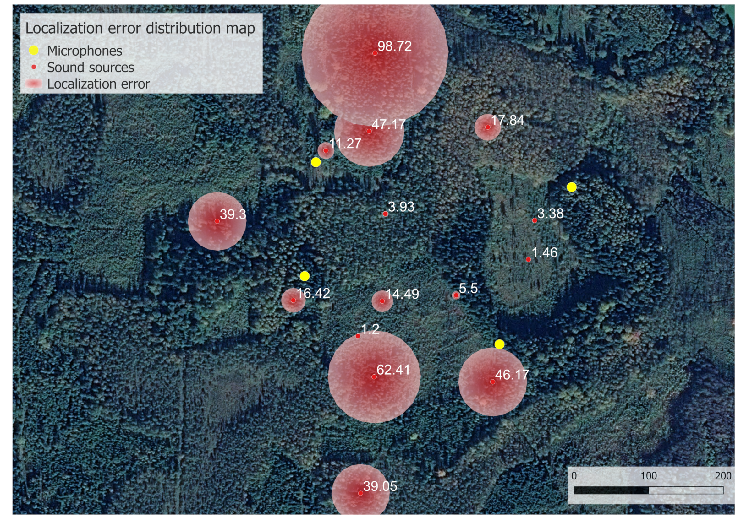
A localization error distribution map for the best-performing
Spectral 2 stage approach is shown in
Figure 10. The median error within the microphone grid was 4 m with a standard deviation of 5 m, but outside the grid it was 39 m with a standard deviation of 29 m. The minimal observed error was 1.2 m but the maximal—99 m. Localization error tends to increase with the distance from the sound detectors due to decreasing signal-to-noise rate affecting precise sound delay assessment.
5. Discussion
We have demonstrated a concept for an automated data processing workflow for the detection and localization of red deer stags from acoustic records acquired using microphones with enabled GPS time synchronization. During events of high activity, an hour of recordings can reach >100 deer calls. Manually detecting this amount of calls from four devices can take up to 2 h in real time, and localizing a single deer call takes from 2 to 15 min, depending on proximity to all recorders and the quality of the spectrogram. In contrast, the proposed automatic detection and localization method reduces the required time for processing 1 h of data to <10 min. In this case, the automated processing is more than 30 times faster and makes this approach useful for animal monitoring. The lack of automation in data processing has been mentioned as one of the main drawbacks in the wider uptake of acoustic sensors in wildlife monitoring [
8,
9].
Previous studies of deer vocal rutting were mainly focused on deer call detection and quantification of acoustic records where GPS time-sync data are not required. We had to acquire our dataset using GPS time-synchronized recorders to perform the study on automated deer localization. As a result, a unique red deer rutting call dataset from four recorders from September 2021 is available with more than 800 annotated deer calls. It was used for training and validation of deer call detection algorithms as well as testing localization approaches. The availability of open acoustic datasets of red deer rut calls, especially from multiple recorders with GPS time synchronization, remains a challenge. The cost of commercially available off-the-shelf devices with GPS time-sync receivers is more than EUR 1000, thus requiring sufficient initial investment in hardware to start such studies and limiting the uptake. Popular choices are SongMeter SM4TS from WildLife Acoustics and BAR-LT from Frontier Labs. However, low-cost solutions presented in recent studies (AudioMoth [
31,
32] and Kinabalu Recorder [
33] without GPS time synchronization for less than EUR 100; CARACAL [
34] with GPS time synchronization for less than EUR 400) could make passive acoustic monitoring more accessible.
Detection of target animal calls together with the noise reduction are the first steps in the data processing workflow where promising results have been demonstrated in previous studies [
8,
9]. Reby et al. [
16] achieved 93.5% accuracy in the identificationof red deer calls during the rut using an approach based on hidden Markov models. This study, as well as end-user requirements, set the accuracy threshold for red deer call detection to 90%. Five commonly used supervised algorithms for target sound detection (SVM, LDA, DT, kNN, and LSTM) were tested and all of them demonstrated accuracy of >90%. The SVM-based approach showed the best performance with the detection accuracy of 96.46% and was implemented in the data processing workflow. Relatively simple machine learning algorithms were chosen due to the limited training dataset. Training of more sophisticated methods such as deep learning neural networks requires much larger reference datasets with minimum of several thousand annotated deer calls. If given a pretrained model in audio classification, transfer learning might be viable with several hundred annotated deer calls. It would be an option if more simple algorithms would fail to achieve the desired performance.
There was no consensus from reviewed studies on the noise-reduction approach that should be applied. The drawback of noise reduction might be a loss of useful information if an inappropriate approach is used; therefore, it was decided to avoid noise reduction if it is not needed to achieve >90% detection accuracy. We tested the performance of red deer call detection with and without the application of 150 Hz high-pass filter to reduce the impact of the wind. However, we did not see a significant impact on the detection accuracy. The application of the HPF resulted in a 3% increase in deer call detection accuracy; therefore, it was implemented in the workflow. It should be noted that detection accuracy would exceed 90% using an SVM-based classifier even without the application of a 150 Hz high-pass filter for noise reduction. Automation of sound delay assessment from multiple microphone records with GPS time synchronization is the most challenging task in automated sound source localization and has limited its application in wildlife monitoring [
8]. Our results have demonstrated that automated sound delay assessment approaches outperform manual assessment performed by a human expert. The best-performing
Spectral 2 stage approach resulted in median localization error of 16 m which was 2.5 times smaller if compared to manual assessment, where median error was 43 m. Sound spectral patterns (even for controlled tests) usually appear as blurred lines without pronounced start and end borders; therefore, it is a challenging task to find the exact sound pattern in each microphone recording. It should be noted that 1 ms error in sound delay assessment causes 0.343 m error in sound source localization, but this error can exponentially increase depending on the location of the sound source relative to the recorders. Nevertheless, the demonstrated localization accuracy obtained using
Spectral 2 stage approach is more than satisfactory for red deer stag monitoring during the rut. The obtained median error of 16 m is in range with the GPS position error (5…20 m) in a forested terrain using standard GPS devices. Localization error estimation was performed using sharp sounds; therefore, it might not represent the localization error of red deer stags. As a next step, the proposed localization approach should be tested on red deer calls with known source locations. It is suggested to perform controlled tests with artificially created or recorded and played red deer calls during further studies.
Wind can increase or decrease the speed of sound, especially upwind and downwind, which is blowing parallel to the line of sight between the sound source and the recorder. In this study we did not account for the potential speed of sound shifts caused by wind direction and speed; therefore speed of sound was assumed to be constant in hyperbolic triangulation calculations. The wind might also increase the noise level, thus decreasing the detectability of red deer calls in all microphones. Reflection and reverberation of sound waves from physical obstacles such as vegetation and topographic relief can also reduce the accuracy of animal localization. The impact of wind and obstacles on detection and localization performance was not evaluated in this study; however, it would be worthwhile to include it in the scope of future research.
The proposed concept for automated data processing workflow for red deer call detection might foster the uptake of passive acoustic monitoring not only in red deer rut monitoring. It might provide a more detailed insight into the rut of red deer. Proposed techniques for detection and localization of target animal sounds could be applied also to other animal species.
6. Conclusions
Acoustic recorders with GPS time synchronization could be used to track red deer stag activities during the rutting season; however, manual data analysis is time-demanding. Data processing automation can speed up data analysis by more than 30 times, thus making such a monitoring approach feasible.
It was demonstrated that >90% red deer call detection accuracy could be achieved with frequently used supervised algorithms applied to spectral features extracted from acoustic signals. However, the best detection performance of 96.46% was demonstrated by the SVM-based approach.
For sound delay assessment in multiple microphones, a novel approach based on cross-correlation and spectral feature similarity was proposed, resulting in a median localization error of 16 m, thus providing a solution for automated sound source localization—the main challenge in data processing workflow automation. The automated method outperformed a human expert’s manual sound delay evaluation, which had a median localization error of 43 m.
Author Contributions
Conceptualization, E.A., G.S., J.O., G.A. and D.J.; Data curation, A.V., J.F., A.B., G.S. and G.D.; Formal analysis, E.A., A.V., G.D., G.A. and D.J.; Funding acquisition, D.J.; Investigation, J.F., A.B., G.S., G.A. and D.J.; Methodology, E.A., A.V., J.O., G.A. and D.J.; Project administration, J.F., A.B., J.O. and D.J.; Resources, G.S., G.A. and D.J.; Software, E.A., A.V. and G.A.; Supervision, J.O., G.A. and D.J.; Validation, A.V., J.F., A.B. and G.D.; Visualization, E.A. and A.V.; Writing—original draft, E.A., A.V. and D.J.; Writing—review & editing, J.F., A.B., G.S., G.D., J.O. and G.A. All authors have read and agreed to the published version of the manuscript.
Funding
The study was performed within the project «ICT-based wild animal census approach for sustainable wildlife management» (1.1.1.1/18/A/146) co-funded by the European Regional Development Fund 1.1.1.1. measure “Support for applied research”.
Institutional Review Board Statement
Not applicable.
Informed Consent Statement
Not applicable.
Data Availability Statement
Information about obtaining the dataset can be requested by contacting D. Jakovels at
[email protected].
Conflicts of Interest
The authors declare no conflict of interest. The funders had no role in the design of the study; in the collection, analyses, or interpretation of data; in the writing of the manuscript, or in the decision to publish the results.
Abbreviations
The following abbreviations are used in this manuscript:
| DOA | Direction-of-arrival |
| DT | Decision tree |
| ERB | Equivalent rectangular bandwidth |
| FSIM | Feature-based similarity index |
| GPS | Global positioning system |
| GTCC | Gammatone cepstral coefficients |
| ISSM | Information theoretic-based statistic similarity measure |
| KNN | K-nearest neighbors algorithm |
| LDA | Linear discriminant analysis |
| LSTM | Long short-term memory |
| MFCC | Mel frequency cepstral coefficients |
| PAM | Passive acoustic monitoring |
| SNR | Signal-to-noise ratio |
| PSNR | Peak signal-to-noise ratio |
| RMSE | Root mean square error |
| SSIM | Structural similarity index |
| STD | Standard deviation |
| SVM | Support vector machine |
References
- Blumstein, D.T.; Mennill, D.J.; Clemins, P.; Girod, L.; Yao, K.; Patricelli, G.; Deppe, J.L.; Krakauer, A.H.; Clark, C.; Cortopassi, K.A.; et al. Acoustic monitoring in terrestrial environments using microphone arrays: Applications, technological considerations and prospectus. J. Appl. Ecol. 2011, 48, 758–767. [Google Scholar] [CrossRef]
- Buxton, R.T.; McKenna, M.F.; Clapp, M.; Meyer, E.; Stabenau, E.; Angeloni, L.M.; Crooks, K.; Wittemyer, G. Efficacy of extracting indices from large-scale acoustic recordings to monitor biodiversity. Conserv. Biol. 2018, 32, 1174–1184. [Google Scholar] [CrossRef] [PubMed]
- Guo, S.; Qiang, M.; Luan, X.; Xu, P.; He, G.; Yin, X.; Xi, L.; Jin, X.; Shao, J.; Chen, X.; et al. The application of the Internet of Things to animal ecology. Integr. Zool. 2015, 10, 572–578. [Google Scholar] [CrossRef] [PubMed]
- Gibb, R.; Browning, E.; Glover-Kapfer, P.; Jones, K.E. Emerging opportunities and challenges for passive acoustics in ecological assessment and monitoring. Methods Ecol. Evol. 2019, 10, 169–185. [Google Scholar] [CrossRef] [Green Version]
- Darras, K.; Batáry, P.; Furnas, B.J.; Grass, I.; Mulyani, Y.A.; Tscharntke, T. Autonomous sound recording outperforms human observation for sampling birds: A systematic map and user guide. Ecol. Appl. 2019, 29, e01954. [Google Scholar] [CrossRef] [Green Version]
- Kalan, A.K.; Mundry, R.; Wagner, O.J.; Heinicke, S.; Boesch, C.; Kühl, H.S. Towards the automated detection and occupancy estimation of primates using passive acoustic monitoring. Ecol. Indic. 2015, 54, 217–226. [Google Scholar] [CrossRef]
- Stevenson, B.C.; Borchers, D.L.; Altwegg, R.; Swift, R.J.; Gillespie, D.M.; Measey, G.J. A general framework for animal density estimation from acoustic detections across a fixed microphone array. Methods Ecol. Evol. 2015, 6, 38–48. [Google Scholar] [CrossRef]
- Rhinehart, T.A.; Chronister, L.M.; Devlin, T.; Kitzes, J. Acoustic localization of terrestrial wildlife: Current practices and future opportunities. Ecol. Evol. 2020, 10, 6794–6818. [Google Scholar] [CrossRef]
- Sugai, L.S.M.; Silva, T.S.F.; Ribeiro, J.W., Jr.; Llusia, D. Terrestrial passive acoustic monitoring: Review and perspectives. BioScience 2019, 69, 15–25. [Google Scholar] [CrossRef]
- Sugai, L.S.M.; Desjonqueres, C.; Silva, T.S.F.; Llusia, D. A roadmap for survey designs in terrestrial acoustic monitoring. Remote Sens. Ecol. Conserv. 2020, 6, 220–235. [Google Scholar] [CrossRef] [Green Version]
- McComb, K. Roaring by red deer stags advances the date of oestrus in hinds. Nature 1987, 330, 648–649. [Google Scholar] [CrossRef]
- Volodin, I.A.; Volodina, E.V.; Golosova, O.S. Automated monitoring of vocal rutting activity in red deer (Cervus elaphus). Russ. J. Theriol. 2016, 15, 91–99. [Google Scholar] [CrossRef]
- Rusin, I.Y.; Volodin, I.A.; Sitnikova, E.F.; Litvinov, M.N.; Andronova, R.S.; Volodina, E.V. Roaring dynamics in rutting male red deer Cervus elaphus from five Russian populations. Russ. J. Theriol. 2021, 20, 44–58. [Google Scholar] [CrossRef]
- Enari, H.; Enari, H.; Okuda, K.; Yoshita, M.; Kuno, T.; Okuda, K. Feasibility assessment of active and passive acoustic monitoring of sika deer populations. Ecol. Indic. 2017, 79, 155–162. [Google Scholar] [CrossRef]
- Enari, H.; Enari, H.S.; Okuda, K.; Maruyama, T.; Okuda, K.N. An evaluation of the efficiency of passive acoustic monitoring in detecting deer and primates in comparison with camera traps. Ecol. Indic. 2019, 98, 753–762. [Google Scholar] [CrossRef]
- Reby, D.; André-Obrecht, R.; Galinier, A.; Farinas, J.; Cargnelutti, B. Cepstral coefficients and hidden Markov models reveal idiosyncratic voice characteristics in red deer (Cervus elaphus) stags. J. Acoust. Soc. Am. 2006, 120, 4080–4089. [Google Scholar] [CrossRef] [Green Version]
- Heinicke, S.; Kalan, A.K.; Wagner, O.J.; Mundry, R.; Lukashevich, H.; Kühl, H.S. Assessing the performance of a semi-automated acoustic monitoring system for primates. Methods Ecol. Evol. 2015, 6, 753–763. [Google Scholar] [CrossRef]
- Digby, A.; Towsey, M.; Bell, B.D.; Teal, P.D. A practical comparison of manual and autonomous methods for acoustic monitoring. Methods Ecol. Evol. 2013, 4, 675–683. [Google Scholar] [CrossRef]
- Aide, T.M.; Corrada-Bravo, C.; Campos-Cerqueira, M.; Milan, C.; Vega, G.; Alvarez, R. Real-time bioacoustics monitoring and automated species identification. PeerJ 2013, 1, e103. [Google Scholar] [CrossRef] [Green Version]
- Mac Aodha, O.; Gibb, R.; Barlow, K.E.; Browning, E.; Firman, M.; Freeman, R.; Harder, B.; Kinsey, L.; Mead, G.R.; Newson, S.E.; et al. Bat detective—Deep learning tools for bat acoustic signal detection. PLoS Comput. Biol. 2018, 14, e1005995. [Google Scholar] [CrossRef] [Green Version]
- Pavlovs, I.; Aktas, K.; Avots, E.; Vecvanags, A.; Filipovs, J.; Brauns, A.; Done, G.; Jakovels, D.; Anbarjafari, G. Ungulate Detection and Species Classification from Camera Trap Images Using RetinaNet and Faster R-CNN. Entropy 2022, 24, 353. [Google Scholar]
- Cristianini, N.; Shawe-Taylor, J. An Introduction to Support Vector Machines and Other Kernel-Based Learning Methods; Cambridge University Press: Cambridge, UK, 2000. [Google Scholar]
- Fisher, R.A. The use of multiple measurements in taxonomic problems. Ann. Eugen. 1936, 7, 179–188. [Google Scholar] [CrossRef]
- Hart, P.E.; Stork, D.G.; Duda, R.O. Pattern Classification; John Wiley & Sons: Hoboken, NJ, USA, 2006. [Google Scholar]
- Li, B.; Friedman, J.; Olshen, R.; Stone, C. Classification and regression trees. Biometrics 1984, 40, 358–361. [Google Scholar]
- Hochreiter, S.; Schmidhuber, J. Long short-term memory. Neural Comput. 1997, 9, 1735–1780. [Google Scholar] [CrossRef]
- Spiesberger, J.L. Hyperbolic location errors due to insufficient numbers of receivers. J. Acoust. Soc. Am. 2001, 109, 3076–3079. [Google Scholar] [CrossRef]
- Watkins, W.A.; Schevill, W.E. Sound source location by arrival-times on a non-rigid three-dimensional hydrophone array. In Deep Sea Research and Oceanographic Abstracts; Elsevier: Amsterdam, The Netherlands, 1972; Volume 19, pp. 691–706. [Google Scholar]
- Murphy, C.; Singh, H. Rectilinear coordinate frames for deep sea navigation. In Proceedings of the 2010 IEEE/OES Autonomous Underwater Vehicles, Monterey, CA, USA, 1–3 September 2010; IEEE: Piscataway, NJ, USA, 2010; pp. 1–10. [Google Scholar]
- Robnik-Šikonja, M.; Kononenko, I. Theoretical and empirical analysis of ReliefF and RReliefF. Mach. Learn. 2003, 53, 23–69. [Google Scholar] [CrossRef] [Green Version]
- Hill, A.P.; Prince, P.; Piña Covarrubias, E.; Doncaster, C.P.; Snaddon, J.L.; Rogers, A. AudioMoth: Evaluation of a smart open acoustic device for monitoring biodiversity and the environment. Methods Ecol. Evol. 2018, 9, 1199–1211. [Google Scholar] [CrossRef] [Green Version]
- Hill, A.P.; Prince, P.; Snaddon, J.L.; Doncaster, C.P.; Rogers, A. AudioMoth: A low-cost acoustic device for monitoring biodiversity and the environment. HardwareX 2019, 6, e00073. [Google Scholar] [CrossRef]
- Karlsson, E.C.M.; Tay, H.; Imbun, P.; Hughes, A.C. The Kinabalu Recorder, a new passive acoustic and environmental monitoring recorder. Methods Ecol. Evol. 2021, 12, 2109–2116. [Google Scholar] [CrossRef]
- Wijers, M.; Loveridge, A.; Macdonald, D.W.; Markham, A. CARACAL: A versatile passive acoustic monitoring tool for wildlife research and conservation. Bioacoustics 2021, 30, 41–57. [Google Scholar] [CrossRef]
| Publisher’s Note: MDPI stays neutral with regard to jurisdictional claims in published maps and institutional affiliations. |
© 2022 by the authors. Licensee MDPI, Basel, Switzerland. This article is an open access article distributed under the terms and conditions of the Creative Commons Attribution (CC BY) license (https://creativecommons.org/licenses/by/4.0/).


 ,
, 


