
A Fusion Method for Multisource Land Cover Products Based on Superpixels and Statistical Extraction for Enhancing Resolution and Improving Accuracy


1
College of Geo-Exploration Science and Technology, Jilin University, Changchun 130026, China
2
Key Laboratory of Land Surface Pattern and Simulation, Institute of Geographic Sciences and Natural Resources Research, Chinese Academy of Sciences, Beijing 100101, China
*
Author to whom correspondence should be addressed.
Remote Sens. 2022, 14(7), 1676; https://doi.org/10.3390/rs14071676
Submission received: 31 January 2022
/
Revised: 19 March 2022
/
Accepted: 19 March 2022
/
Published: 31 March 2022
(This article belongs to the Collection Google Earth Engine Applications)
Abstract
:The discrepancies in existing land cover data are relatively high, indicating low local precision and application limitations. Multisource data fusion is an effective way to solve this problem; however, the fusion procedure often requires resampling to unify the spatial resolution, causing a lower spatial resolution. To solve this problem, this study proposes a multisource product fusion mapping method of filtering training samples and product correction at a fine resolution. Based on the Superpixel algorithm, principal component analysis (PCA), and statistical extraction techniques, combined with the Google Earth Engine (GEE) platform, reliable land cover data were acquired. GEE and machine-learning algorithms correct the unreliable information of multiple products into a new land cover fusion result. Compared to the common method of extracting consistent pixels from existing products, our proposed method effectively removes nearly 38.75% of them, with a high probability of classification error. The overall accuracy of fusion in this study reached 85.80%, and the kappa coefficient reached 0.82, with an overall accuracy improvement of 11.75–24.17% and a kappa coefficient improvement of 0.16 to 0.3 compared to other products. For existing single-category products, we corrected the phenomenon of overinterpretation in inconsistent areas; the overall accuracy improvement ranged from 2.99% to 20.71%, while the kappa coefficient improvement ranged from 0.22 to 0.56. Thus, our proposed method can combine information from multiple products and serve as an effective method for large areas and even as a global land cover fusion product.
1. Introduction
Accurate, large-area land cover maps are basic data support for exploring the relationship between natural and biological activities and spatial patterns [1,2]; the simulation, monitoring, and evaluation of ecological and environmental changes [3]; human social and economic development [4,5]; and other scientific studies. Food security and arable land area assessment, forest change monitoring, urban extent expansion and structure analysis, and water body area extraction and pollution assessment also require timely updates of large thematic maps to provide important indicators for human sustainable development strategies [6,7]. With the development of remote sensing technology and the appearance of a variety of sources of satellite data, remote sensing has become an important method for mapping land cover over a large area [8,9].
Based on image data from NOAA/AVHRR, MODIS, ENXISAT/MERIS, and other satellite sensors, land cover products usually have a coarse spatial resolution (300–1000 m). For example, we have 500 m spatial resolution MODIS global land cover data from Boston University [8]. The European Space Agency (ESA) ESA-CCI dataset has a 300 m spatial resolution [10]. The Copernicus Global Land Service (CGLS) dataset has a 100 m spatial resolution [11]. Previous research has shown that a lower spatial resolution usually leads to lower accuracy [12,13]. With the development of the Landsat series of satellites, the monitoring of a large area with medium-spatial-resolution land cover products became possible. For example, FROM-GLC, developed by Tsinghua University in China [14], and GlobeLand30, developed by the National Basic Geographic Information Center of China, etc., have 30 m spatial resolution [15]. In addition, there are a number of single-category land cover products, such as the Global Food Security support analysis data 30 m (GFSAD30) developed by USGS [16], the Advanced Land Observing Satellite Phased Array L-band SAR (PALSAR) developed by the Japan Aerospace Exploration Agency (JAXA)) [17], the Global Surface Water Explorer dataset [18], etc. Different remote sensing images affect the spatial resolution of land cover data, and the spatial resolution restricts the level of detail of a land cover classification system [19]. Consequently, due to different classification systems, classification methods, and types of satellite sensors, there is great inconsistency between multisource products. When multisource products are used in collaboration, it will lead to greater uncertainty [16,20].
Data fusion can overcome the limited accuracy and uncertainty associated with single data sources by integrating multisource data [21,22]. Some fusion decision methods, such as the Bayesian theory, Dempster–Shafer evidence theory, and fuzzy set theory have been effectively applied in numerous studies [20,23,24]. Several studies have introduced multisource statistics to calibrate fused products, which can improve the accuracy of fusion results. The accuracy of the original products significantly affects the fusion results [25,26], such that, as input products increase, the weights of the products are determined with a priori knowledge; otherwise, it is difficult to obtain good results [27]. Due to the above limitations of fusion decision methods, researchers selected samples from previous surface coverage products to update maps. For example, the U.S. Geological Survey (USGS) proposed spectral change monitoring methods to identify nonchange areas and used these areas as samples to train decision tree classifiers that can rapidly update land cover maps [28]. However, information obtained from a single source of surface coverage products is often less reliable than the fusion of multiple products [21].
Multisource data fusion often requires resampling to unify spatial resolution and obtain consistent areas [16]. Consistent areas are defined as areas in which a variety of land cover products remain in the same category at the same geographical location [29]. We can usually have a high level of confidence in the information retained about each ground cover product [27]. Therefore, extracting effective information from the consistent areas of multi-source products and correcting the inconsistent areas is considered a fusion method to effectively improve mapping accuracy [30]. However, due to resampling, the final result will still have a coarse spatial resolution.
To solve the above problems, we base this study on an existing method [31] and further propose a multisource land cover products fusion method based on superpixels and statistical extraction that achieves fine spatial resolution and high-accuracy fusion results. In the first step, we analyze the consistency of multiple products to divide the study area into 300 m spatial resolution (coarse) consistent areas and inconsistent areas and compose a 30 m feature image layer on the GEE platform. In the second step, the PCA and SNIC (simple noniterative clustering) algorithm is used to segment the image in the coarse consistent areas, remove outlying pixels, and obtain 30 m spatial resolution (fine) consistent areas. In the third step, we obtain reliable training samples by the local adaptation sampling method and correct inconsistent areas by machine learning to generate fine spatial resolution and high-precision fusion results. Then, we apply and verify the proposed method with the example of southeast Asia.
2. Materials
2.1. Study Area
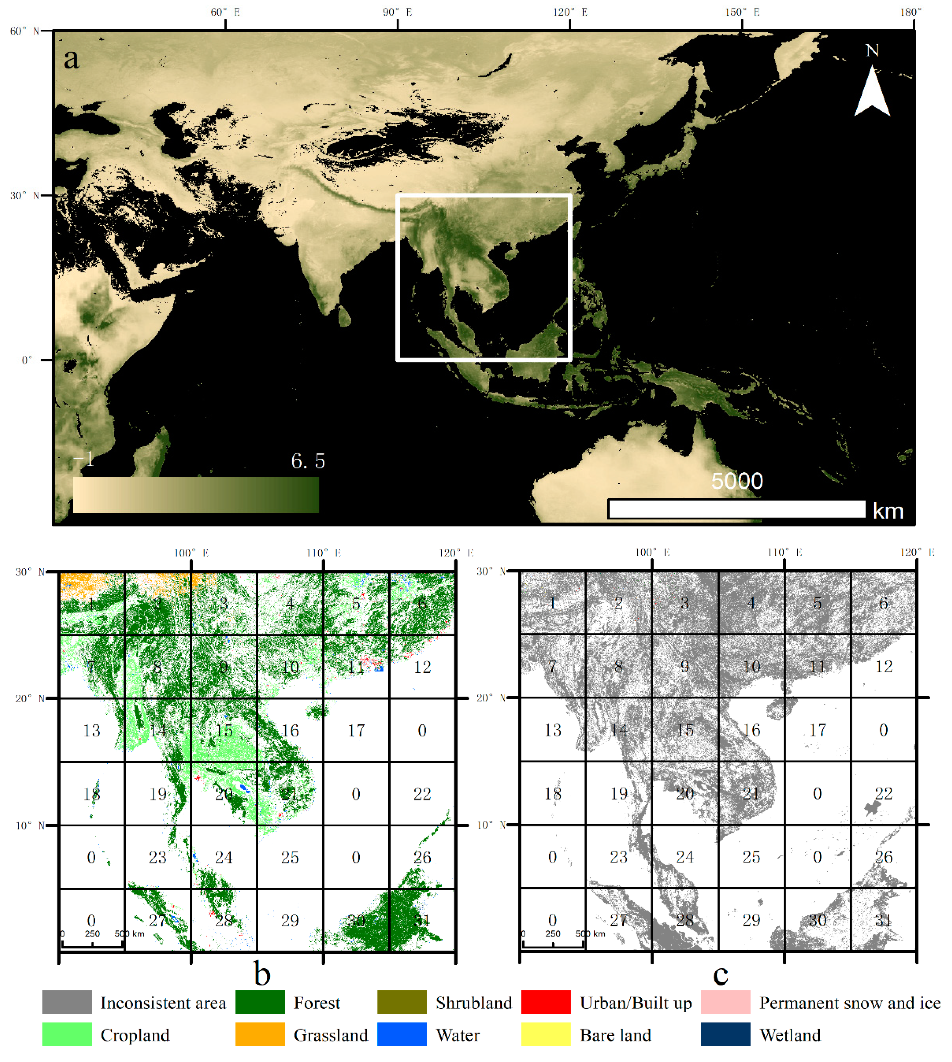
The study area is located between 30°N and the Equator and between 90°E and 120°E, spans an area of about 5 million km2 (Figure 1a), and consists of tropical and subtropical ecosystems that have rich biodiversity. Figure 1a shows that the net primary productivity (NPP) is very high in this part of the northern hemisphere at low and mid-latitudes. The NPP and biodiversity significantly affect the population density of an area [32]. Most of the study area is occupied by cropland and forest; cropland expansion and forest loss are very common in this region [33]. This creates a complex land cover pattern in this region, such that accurate land cover products are needed to provide data to support various scientific studies, as the current land cover products covering this region exhibit poor consistency and generate uncertain information when used in concert, as detailed in Section 2.2.1. Thus, a reliable method is needed to fuse various surface covering products to yield a high-accuracy and uniform product.
Differences in location can cause huge variations in the spectral reflectance of various features, which are more pronounced for climate-influenced features (e.g., cropland and grassland) [34]. Furthermore, there is a significant difference in the feature distribution within a local area compared to the entire study area, and this difference can have an impact on accuracy when selecting samples [35]. At the same time, the area per interpretation must be reduced to ensure that the running memory of the GEE is not exceeded. Therefore, this study divided the study area into 31 tiles of 5° × 5°, as shown in Figure 1b, where the tile numbered 0 was not involved in the consistency analysis due to the small land area (Section 2.2.1). Samples were selected from corresponding or adjacent tiles as much as possible to minimize the effect of latitude and longitude differences, as detailed in Section 3.3.
2.2. Data Sources and Preprocessing
2.2.1. Uniformity and Consistency Analysis of Multisource Land Cover Products
This study used eight products from the 2015 coverage study area: the Moderate Resolution Imaging Spectroradiometer Land Cover Type Product (MCD12Q1), CCI-LC, Copernicus Global Land Service (CGLS), FROM-GLC, GFSAD30, PALSAR, Global Surface Water Data (GSWD), and Global Human Settlement Layer Built-up area (GHS-BUILT). Product details are listed in Table 1. We unified the eight products under the same geographical coordinate system (WGS84, World Geodetic System 1984), along with spatial resolution unification, to facilitate multisource data fusion. In previous studies, data spatial resolution unification was often performed by selecting a coarse spatial resolution for all products as the target of resampling to optimally control the product accuracy. Considering that only one of the eight products (MCD12Q1) has a spatial resolution of 500 m, followed by 300 m, resampling to 300 m can preserve the maximum amount of detail. Nearest neighbor is the resampling technique to be used, determined by referring to previous studies. The definitions of classification systems of the eight products varied due to different producers and sensors, and we integrated the classification systems of each product to finally classify it into one of the nine ground cover categories (Figure 1b). Further details on the classification systems are provided in the literature and S 1 [31].
The consistency level is defined as the number of land cover products that are consistent with a category at the location of an image. A higher consistency level represents a higher confidence level for the corresponding category [27]. The method of consistency area generation in this study is the same as in Liu and Xu [31]. The pixels of the highest consistency level for each category were selected as the consistent area of each category (Figure 1b). The rest is called inconsistent area (Figure 1c), amounting to about 55.3%. Notice that the consistent area here is 300 m spatial resolution, and we call it the coarse consistent area. Because 30 m spatial resolution land cover products have more detail, the coarse consistent areas ignore this detail, which limits the application. At the same time, incorrectly marked pixels will provide incorrect samples, limiting the sampling accuracy.
2.2.2. Landsat Data Composition
In this paper, 30 m spatial resolution Landsat images were selected to reinterpret the inconsistent areas. The screening of images for cloud-free pixels and cloud masking on the GEE platform revealed that the images from 2015 were not sufficient to cover the entire study area, such that Landsat images from the years adjacent to 2015 (2014 and 2016) were selected to fill in the gaps in the data. The orthocorrected surface reflectance data from the Earth observation satellite 7 ETM+ and 8 OLI sensors covering the study area for the three years 2014–2016 were screened for a total of 27,223 images, including 11,278 Landsat 7 ETM+ and 15,945 Landsat 8 OLI. Invalid observations due to clouds, cloud shadows, and snow in each image were masked by the FMASK algorithm available on the GEE platform [36,37]. The use of Landsat 7 data in the long time series was similarly used to fill in the gaps in the data and increase the frequency of valid observations. Furthermore, Roy et al. found potentially subtle but significant differences between the spectral features of Landsat ETM + and Landsat 8OLI. Hence, we applied the coefficients proposed by Roy et al. to achieve reconciliation by linearly converting the ETM + spectral space to the OLI spectral space [38].
Six spectral bands, namely, blue, green, red, near-infrared (NIR), shortwave infrared (SWIR)1, and SWIR2 are used in Landsat 7 ETM+ and Landsat 8 OLI, and 11 spectral indices are calculated, with the formulae for each spectral index shown in Table 2 [39]. Referring to previous research to ensure adequate phenological information and image quality, the year was divided into three periods (period 1: 1–120 days in 2015, period 2: 121–240 days in 2015, and period 3: 241–365 days in 2015) [31,35]. We used the median pixel of the time series of each period as the spectral feature of this period, because the median in time series is insensitive to phenological change [40]. To increase the discrimination of the features, we also calculated the standard deviation of each feature for three years, such that a total of 68 band feature layers ((6 bands +11 spectral indices) × 3 periods + (17) three-year standard deviation) were synthesized on the GEE platform by each tile.
3. Methods
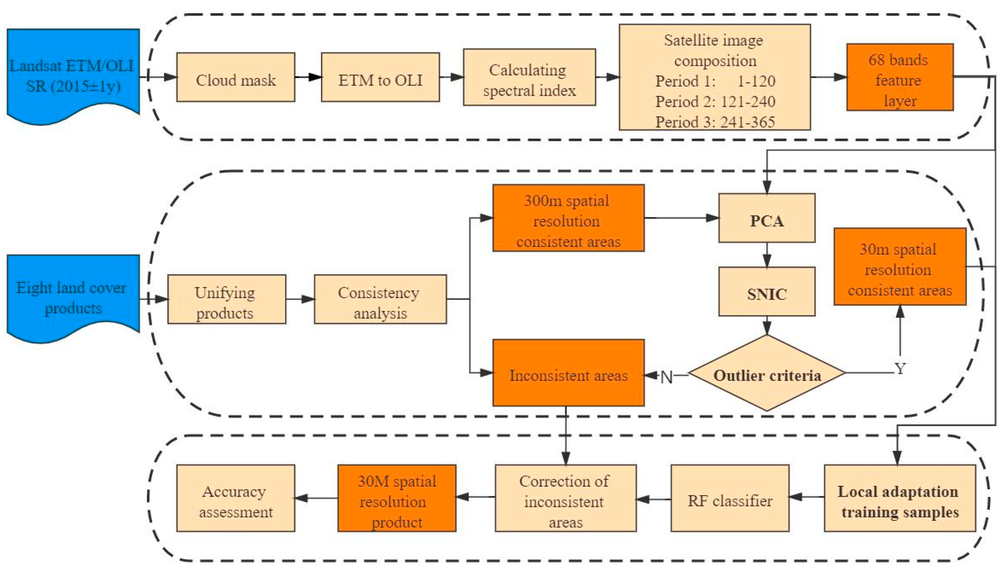
Figure 2 shows the flowchart of the process used in this study to realize the multisource land cover products fusion method. The method is divided into three main parts. First, Landsat ETM and OLI images in the study area were retrieved on GEE and then preprocessed to create a composite image layer. Second, PCA technology was used to reduce the dimension of 68 bands, the SNIC algorithm was used to segment the image layer in the coarse consistent area, and the outlier pixels were removed by a statistical method. Finally, a large number of reliable training samples was obtained in the 30 m spatial resolution consistent area by the local adaptation sampling method, and we reinterpreted inconsistent areas and evaluated accuracy. Validation of the results was performed by sample points of high spatial resolution images, visually interpreted by Google Earth.
3.1. Principal Component Analysis of Coarse Consistent Areas
A lot of research determines whether each pixel has changed from an existing land use cover product by the anomalous distribution of spectral features [28,53]. This study applies this method to purify samples in coarse consistent areas (Figure 1b). Spectral features used for statistical distributions generally consist of multiple metrics, such as Zhang et al., using the pixel with the smallest distance from the mean of 39 metrics as a sample [35], because there is no single metric that can distinguish multiple features, and outlier detection for multiple metrics is a complex matter. In this study, we employed the PCA technique for the feature reconstruction of 68 bands of feature layers to regenerate PC1-68 bands, where the first principal component (PC1) can be equivalently defined as the direction that maximizes the variance of the projected data and decreases sequentially thereafter [50]. Through this approach, each feature can be distinguished by fewer bands, achieving data dimensionality reduction. We performed PCA for consistent areas within each tile separately, and this step was executed on the GEE.
3.2. Superpixel Removal of Coarse Consistent Areas
Multisource data preprocessing and resampling can achieve the coarse consistent area. In fact, data such as Landsat images can already provide more detailed results. Hence, we aimed to purify the coarse consistent area and improve it to fine resolution. Then, we extracted effective information from the initially obtained fine consistent areas and applied 30 m spatial resolution Landsat images provided by GEE to correct the uncertainty information between multiple sources [31].
However, pixel-by-pixel removing will produce a large number of speckles (the “pretzel phenomenon”) due to the heterogeneity within the image pixels [54], and the counting of a large number of pixels often exceeds the GEE memory limit. A superpixel is a small region composed of a series of adjacent pixels with similar features such as color, brightness, and texture. Most of these small regions retain effective information and generally do not destroy the boundary information of objects in the image. Grouping pixels with certain similar features by a superpixel segmentation algorithm and then removing the pixel groups (superpixel) will greatly reduce the pretzel phenomenon, while avoiding the computational complexity due to redundant information [55]. This study chose the simple noniterative clustering (SNIC) superpixel algorithm provided by GEE, which is an improved version of the simple linear iterative clustering algorithm (SLIC) that does not require iterations, is more efficient, and is better for boundary preservation.
Moreover, SNIC requires a size parameter to determine the seed interval and, considering that the consistent area has 300 m spatial resolution and the Landsat image has 30 m spatial resolution, we experimentally determined the size value to be 3, which is sufficient for oversegmenting the Landsat image in the consistent area, avoiding the impact of insufficient segmentation on the removing of outliers later [56]. We set the compactness parameter in SNIC to 0, which disables spatial distance weighting, as we do not want the generated pixels to be regular compact squares; the aggregation of pixels with similar properties is sufficient for our purposes. The mean of the six original bands of the Landsat image at the median of 2015 was synthesized and used as the band for the input segmentation. The mean values of PC1 and PC2 within each superpixel were computed after SNIC segmentation and used as features of the superpixel instead. By aggregating image elements with the same attributes, the statistical features of each superpixel were made more consistent with the real geographic object, and outliers could be detected more easily [57].
Then, we counted the PC1 and PC2 attributes of the generated superpixel. In general, a threshold for outlier detection is determined empirically or by an optimal threshold search algorithm, and the removed superpixel covered the mislabeled regions in the coarse consistent area [28]. However, coarse consistent areas are multicategory, and if performed simultaneously would lead to under- or overremoving. Therefore, we counted and removed the coarse consistent areas for each category separately. After our tests, PC1 and PC2 of each feature were found to be normally distributed, so we combined PC1 and PC2 and applied the Lajda criterion to construct the outlier discriminant condition:
where represents the ground cover category, represents each superpixel, , represent the PC1, PC2 values of each superpixel in each category, , represent the mean values of PC1, PC2 in each category, and , represent the standard deviation of PC1, PC2 in each category, respectively. According to Morisette and Khorram, who proved that the optimal range of thresholds is the mean value plus or minus 0.5–1.5 times the standard deviation [58], we determined the threshold value, with the standard deviation as the range. The image pixels in the superpixel that satisfy the outlier discrimination condition are then considered to be a fine consistent area; otherwise, they are marked as removed pixels. The removed pixels are merged with the inconsistent areas in Section 2.2.1 to become the final inconsistent areas.
3.3. Local Adaptation Sample Set
As per Section 2.1, the study area is divided into 31 tiles for the above process to reduce the effect of latitude and longitude differences on the reflectance of different features, and we employed a locally adaptive sampling method [35]. Samples for each feature within each tile must first be randomly selected from the fine consistent area within this tile for each category after purification. We only set a lower limit on the number of samples per category (1000), and no upper limit on the total number except meeting the memory limit of GEE operations. If there were insufficient samples in the corresponding tiles due to the lack of fine consistent areas of a certain category or fewer consistent areas, the missing samples were replenished from the nearest surrounding tiles. The selected samples were used to train only the current tiles. The total number of samples was over 300,000; this group is called a locally adapted sample set. Using this locally adapted sampling method can minimize the inconsistency of the characteristic attributes of the categories due to the spatial distribution. Random sampling is generated by generating random points within an exact consistent area.
3.4. Correction of Inconsistent Areas
In this study, the random forest (RF) classifier was trained by the locally adapted training samples of Section 3.3 with the aim of reinterpretation for inconsistent areas. RF is a machine-learning classifier that contains multiple decision trees and whose output class is determined by the plurality of the output classes of the individual trees [59]. In remote sensing, RF has the advantages of being insensitive to noise, avoiding overfitting, and achieving higher accuracy compared to other machine-learning classifiers. Based on previous studies, we chose 300 trees, using 63% of the training data randomly selected to package each tree as parameters for the RF classifier [52,60,61]. The classification results were mosaicked with the fine consistent areas to form a new 30 m spatial resolution land cover fusion result.
3.5. Validation and Accuracy Assessment
To verify the reliability of the extracted samples from the fine consistent area, historical high spatial resolution images in Google Earth were used to validate them. We randomly selected 900 sample points (100 of each category) from the fine consistent area for each category [62], counted the type of each pixel point and the confusion matrix of nine categories, and calculated the accuracy of each point being correctly masked, before and after removing.
Validation and evaluation of the inconsistent areas’ correction results were performed using validation points generated by stratified random sampling, and the validation points were also interpreted by Google Earth. The number of validation points was 1507 (Table 3). Four original spatial resolution multicategory land cover products (MCD12Q1, CCI-LC, CGLS, and FROM-GLC) and four single-category products (GFSAD30, PALSAR, GSWD, and GHS-BUILT) within the study area were also compared and evaluated. Notably, our accuracy evaluation was performed only in the inconsistent area, as the differences in accuracy of various products are mainly reflected there [31]. In contrast, the class distribution of all products in the fine consistent area was the same and completely reliable. We counted the confusion matrix for each product and calculated the commonly used metrics (producer accuracy, user accuracy, and overall accuracy) to evaluate the calibration results and the accuracy of the spatial distribution of the four multicategory products [63,64].
4. Results
4.1. 30 m Spatial Resolution Coarse Consistent Area Removal Results
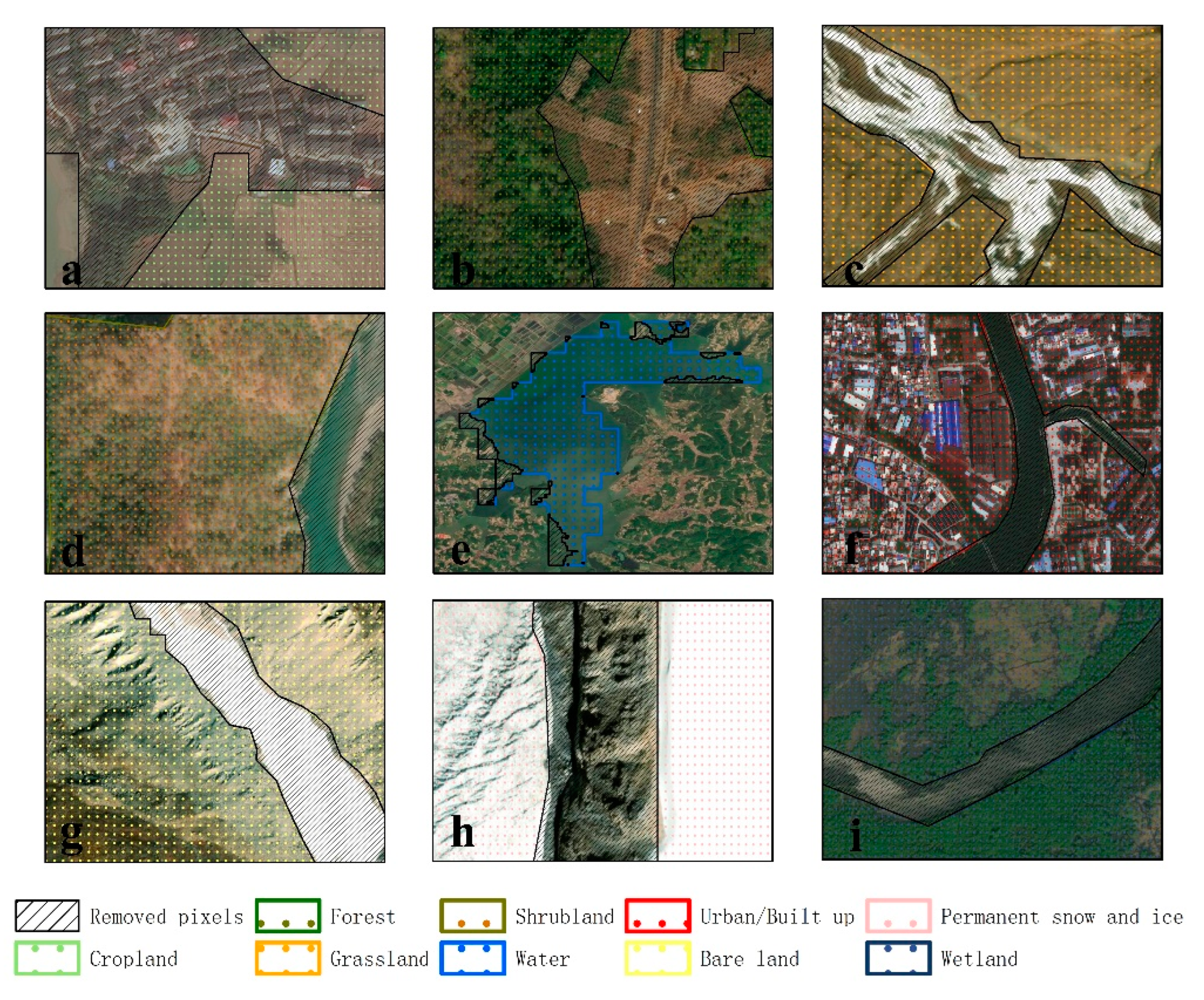
Figure 3a shows the results of superpixel removal. After counting the number of pixels, about 38.75% of them were removed (Figure 3b). Among these, the categories of shrubland, bare land, permanent snow and ice, and wetland required local adaptation samples due to their small incidence and uneven spatial distribution of image elements in the fine consistent area. Figure 4 shows the visual details of the removal results in the enlarged window. From the visual effect, incorrectly marked pixels of nine categories of the coarse consistent area can be effectively removed by the superpixel removal method. Figure 4a shows the coarse consistent area removal results for the cropland, and the corresponding high-definition images can identify that the removed pixels are architectural areas. Figure 4b shows the results of consistent area removal for the forest land, where the pixels removed are roads and bare land in the forests; the pixels removed from the grassland (Figure 4c) are bare land and roads in the grassland; the pixels removed from the shrubland (Figure 4d) are the surrounding bare land; the pixels removed from the consistent area of the water (Figure 4e) are the croplands, grasslands, built-up areas, and bare land around the water; the coarse consistent areas removed from the urban/built-up land (Figure 4f) are the grass, water, and bare land; the coarse consistent areas of bare land (Figure 4g) and permanent snow and ice (Figure 4h) are mixed together at high altitudes. The consistent areas of wetlands (Figure 4i), although less consistent, still remove some pixels that are obviously not wetlands. No pretzel phenomenon is generated in the fine consistent region, because the superpixels are removed instead of individual pixels.
4.2. Validation of Automatic Sample Extraction in Fine Consistent Areas
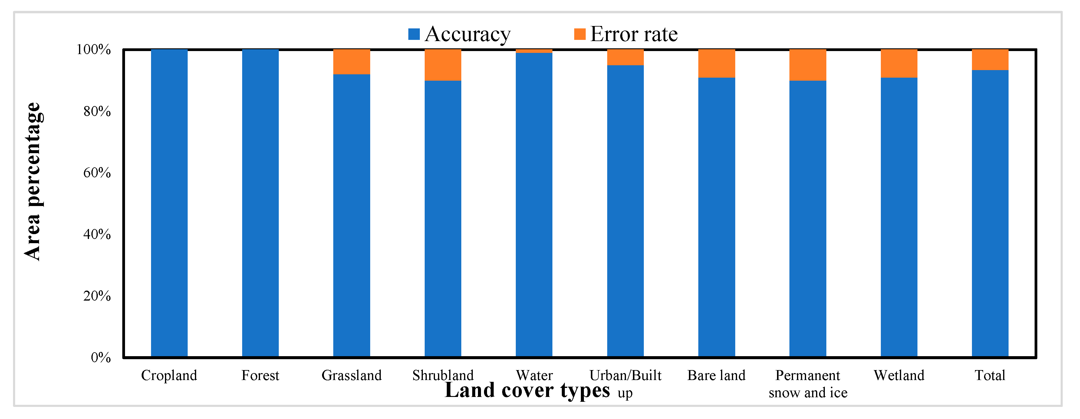
We verified the confusion matrix of the 900 randomly selected samples (Figure 5) shown in Table 4 and found that the accuracy of the samples for shrubland and permanent snow and ice was as low as 90%, the accuracy of the water was as high as 99%, and the overall accuracy of all samples was 93.44%. The confusion matrix shows how the samples in each type are incorrect: for example, the cropland sample contains small amounts of grassland, water, and urban/built-up areas. This indicates that inconsistent feature classes in cropland still exist within the 30 m spatial resolution of the fine cropland consistent area. However, the error rate for each of the selected types of samples does not exceed 10%. From the above verification, we know that the samples selected by our method are reliable and satisfy the threshold requirement that the RF classifier can resist at most 20% of the noise [61].
4.3. Inconsistent Area Correction Results and Accuracy Evaluation
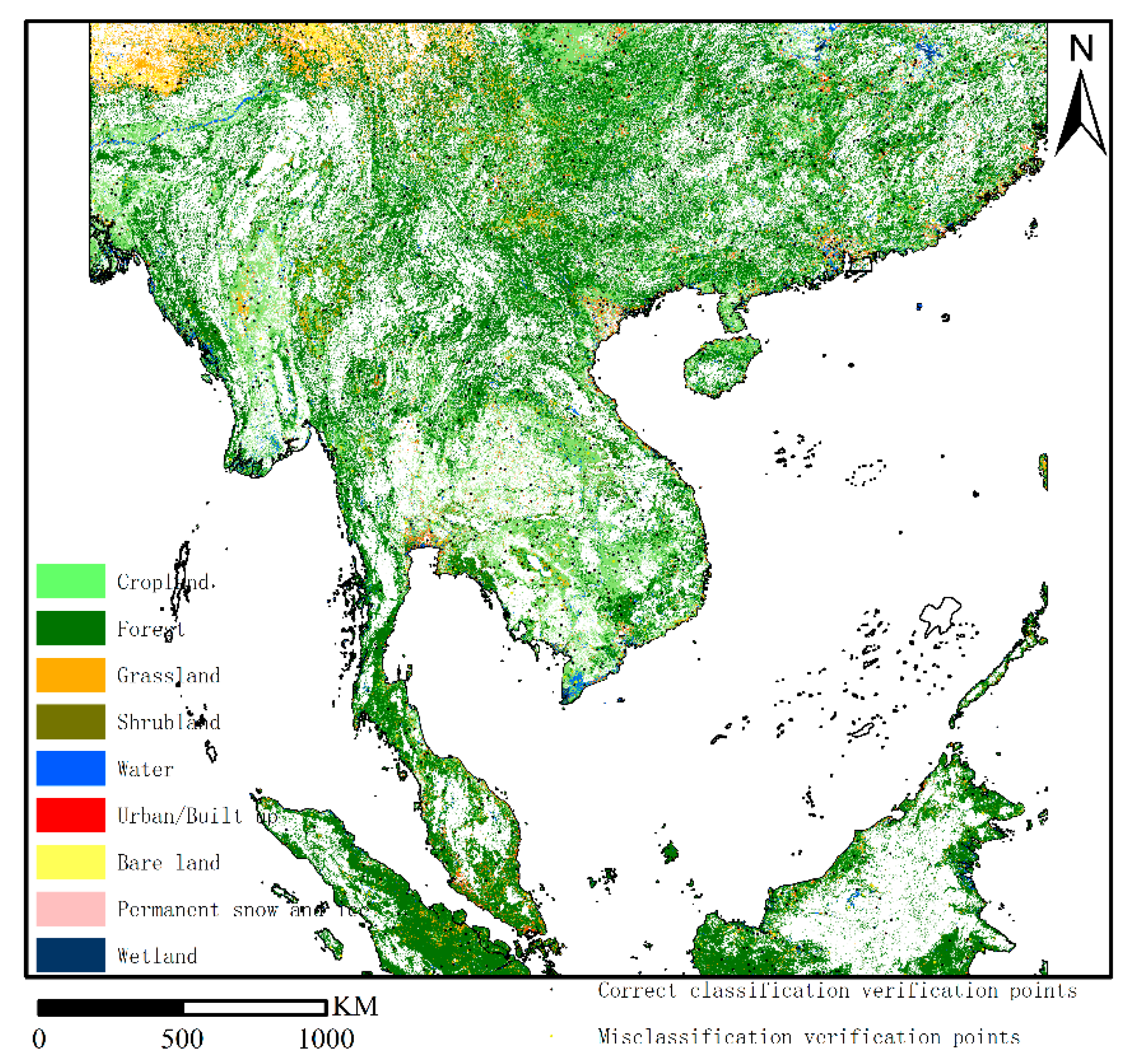
The correction results for the inconsistent areas are shown in Figure 6. The PA, UA, OA, and confusion matrix based on the validation points are shown in Table 5. The overall accuracy of the final correction results is 85.8%, and the kappa coefficient is 0.82. In the validation of PA, the highest PA of forest can reach 91.5%. The PA of shrubland is the lowest, 73.65%. In the validation of UA, urban/built-up area has the highest UA at 94.25%, while wetland has the lowest at 68.97%. The difference between PA and UA represents the reliability of land cover products for the accuracy of land cover types (Li and Xu, 2020). In the correction results, the difference between PA and OA for all types except building land and wetland is within 5%, indicating that the reliability of these types is relatively strong in the results. The difference between PA and UA for building land is 12.25%, which is due to the complex landscape pattern in the urban area, which can easily misclassify urban vegetation into cultivated and grassland types and thus reduce the mapping accuracy of urban/built-up areas. The difference between PA and UA for wetlands is 9.47%, because agricultural land, grassland, and water bodies are easily misinterpreted as wetlands to a certain extent, resulting in low UA for wetland types.
4.4. Comparison with Other Products
4.4.1. Multicategory Product Comparison
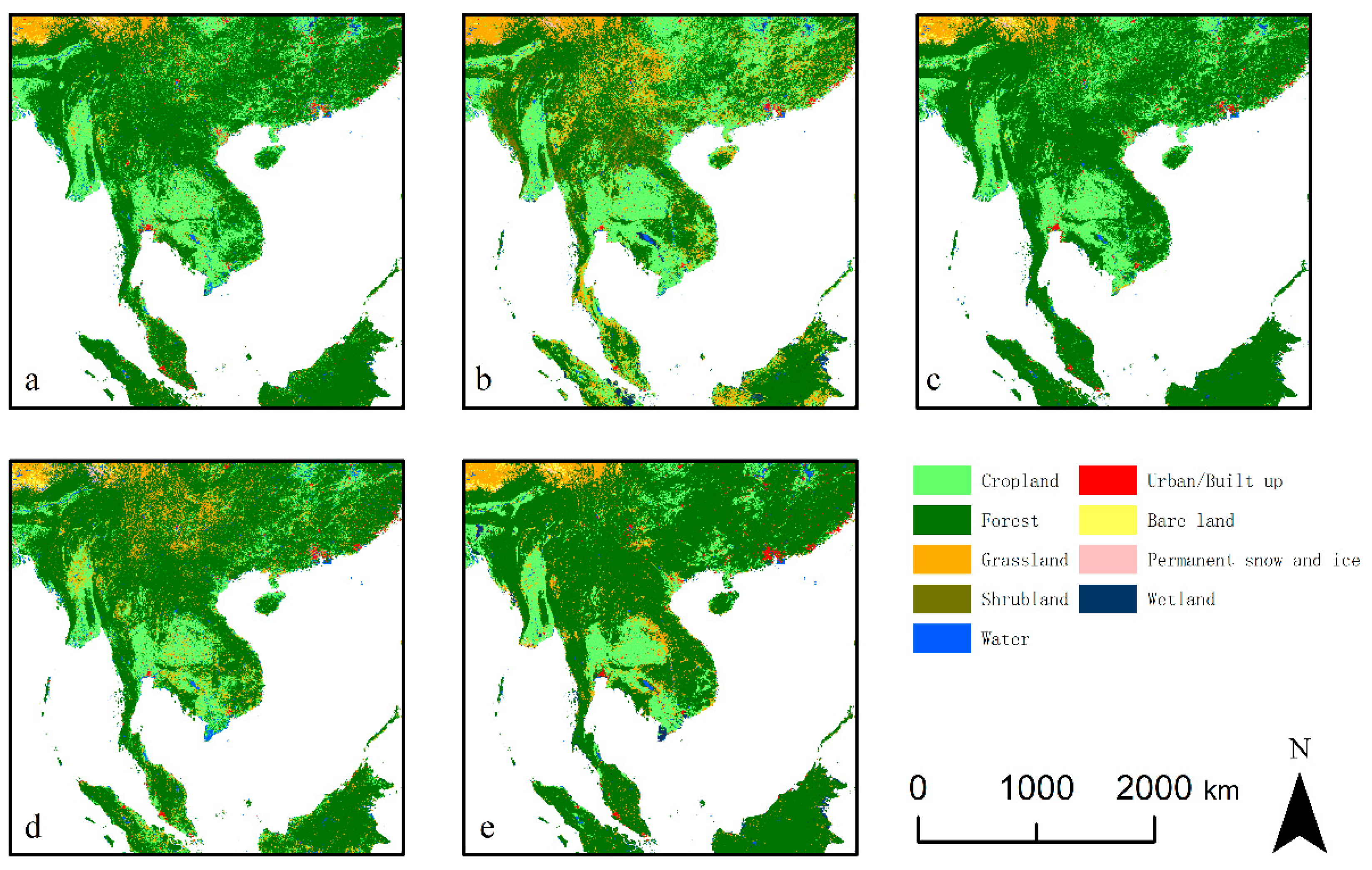
The corrected inconsistent areas were mosaicked with fine consistent areas to obtain the fine spatial resolution land cover fusion results. There were no differences in tiles boundaries, as shown in Figure 7a. The land cover results obtained by the proposed method were somewhat similar in terms of feature class distribution compared to other multicategory products (Figure 7b–e), owing to the consistency of the multiple products included in the method.
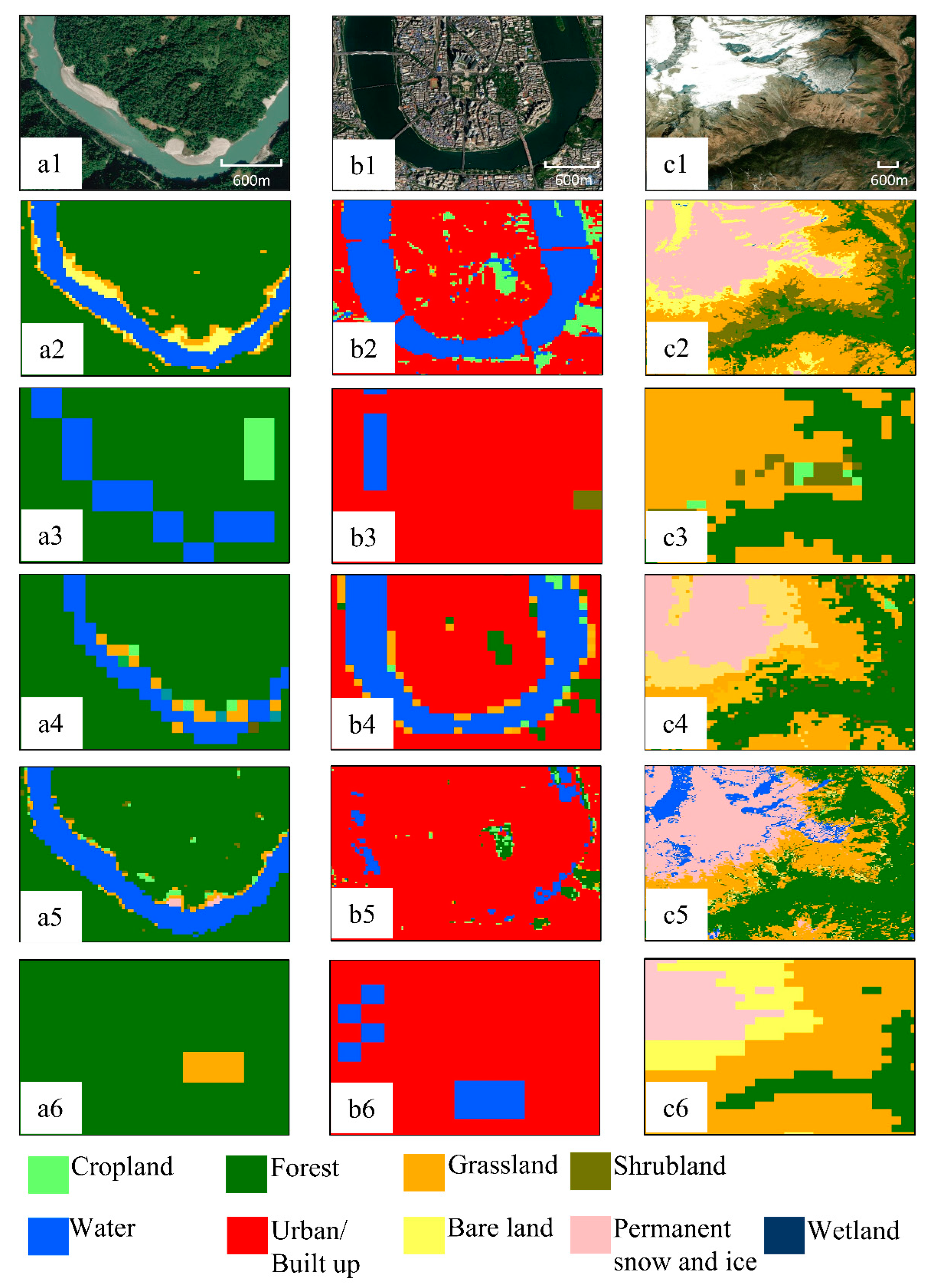
However, the differences in spatial resolution and the mapping methods lead to significant differences in details for each product, as shown in Figure 8. Because the spatial resolution of the three products, CCI-LC, CGLS, and MCD12Q1, is below 30 m, numerous details are missed. For example, some fine rivers (Figure 8(a1)) are completely ignored in these three products (Figure 8(a3,a4,a6)), and even in the coarse spatial resolution MCD12Q1, there is only the forest category. The urban/built-up type is more complex internally (Figure 8(b1)), and the internal information is even more incompletely covered by the urban/built-up type in the coarse spatial resolution products (Figure 8(b3,b4,b6)). Permanent snow and ice, grass, and bare land are not accurately portrayed in coarse spatial resolution products (Figure 8(c3,c4,c6)). FROM-GLC has the same spatial resolution as our fusion result and, although the details are not ignored visually, our land cover product is more accurate at portraying real landforms. For example, many areas of bare land and grassland in Figure 8(a1,a2) are incorrectly marked as cropland in FROM-GLC (Figure 8(a5)), continuous bodies of water (in Figure 8(b1)) are incorrectly marked as buildings in Figure 8(b5), and in Figure 8(c1), the FROM-GLC product incorrectly marks part of the bare land and grassland located in the shadows as water (Figure 8(c5)).
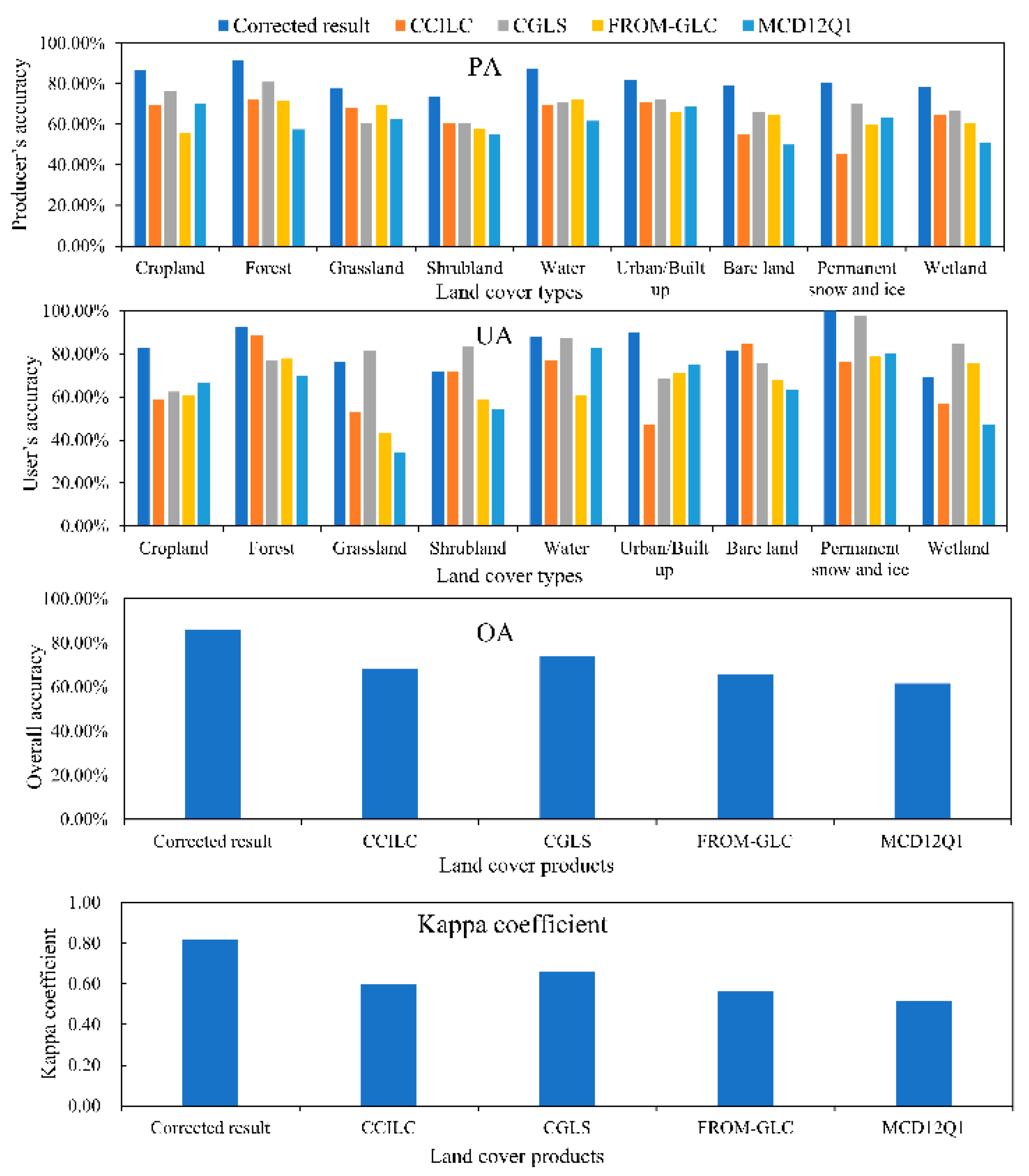
The accuracy assessment results of the verification points of the inconsistent areas for the four multicategory products are shown in Tables S2–S5, and the comparative assessment results of the calibration results and the four products (including PA, UA, OA, and Kappa coefficient) are shown in Figure 9. Figure 9 shows that the PA of each type in our inconsistent region correction result is higher than the other four products. In the comparison of UA, except for grassland, shrubland, and bare land, which are more ill-defined, and wetland, which is difficult to identify, the UA is not the highest. The UA of the other types are all higher than the other four products. Our correction results have the highest OA (85.80%) and kappa coefficient (0.82), the lowest OA for MCD12Q1 (OA is 61.63%, kappa coefficient is 0.52), and the correction results are 11.75–24.17% better than the other products in OA; the kappa coefficient increased by 0.16–0.3. This indicates that the mapping results of our proposed method effectively improve the accuracy of land cover in inconsistent areas.
4.4.2. Single-Category Product Comparison
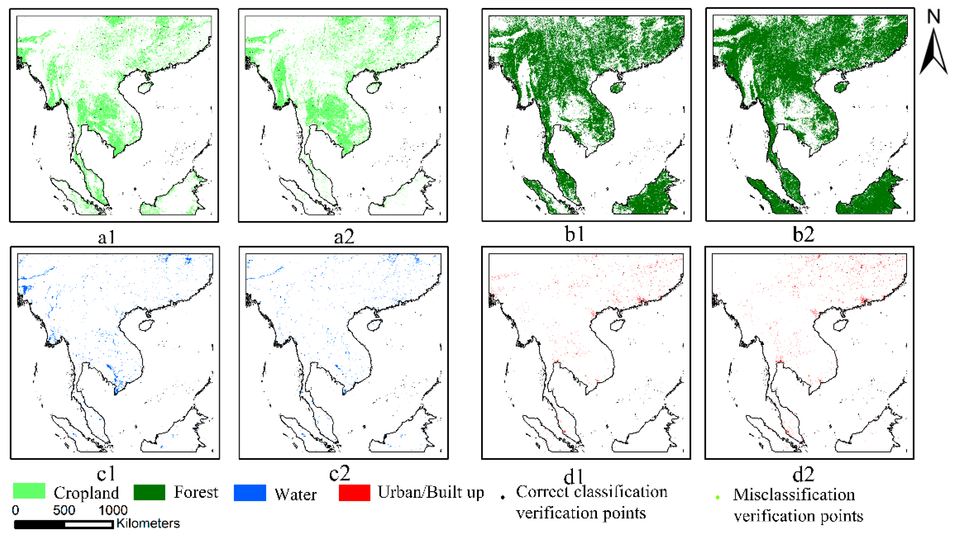
A comparison of the cropland, forest, water, and urban/built-up types in the calibration results with the four single-category products (GFSAD30, PLASAR, GWSD, and GHS-BUILT) is given in Figure 10. The distribution of the corresponding categories in the correction results remains with the four products. The confusion matrices of the correction and validation results of the four single-category inconsistent regions are shown in Tables S6–S13, and the comparative evaluation results are shown in Table 6. Based on the comparison of the accuracy of the corresponding types of categories in the inconsistent areas, the PA of our correction results is closer to the existing single-category products, whereas the UA, OA, and kappa coefficient are higher than those of the corresponding single-category products. The improvement in OA for each type in the inconsistent areas varied, with the largest improvement of 20.71% for forest and the smallest improvement of only 2.99% for water bodies. As to the kappa coefficient, the largest improvement was 0.56 for urban/built-up, and the smallest improvement was 0.22 for water. The results show that our method, nevertheless, slightly improved the accuracy compared to a single category.
5. Discussion
To solve the problem that the fusion result cannot achieve fine spatial resolution due to resampling in previous fusion methods [27,29,30], this study developed a multisource land cover products fusion method based on the SNIC segmentation algorithm and the PCA technique. The results show that this fusion method can obtain fusion results with fine spatial resolution and improve the accuracy of inconsistent areas to various degrees. This method creatively uses the SNIC segmentation algorithm to segment Landsat image layers in the coarse consistent areas into pixel groups, and outlier pixel groups were removed by PCA and statistical methods. Therefore, coarse consistent areas can be purified into fine consistent areas, and the spatial resolution has also been increased by 30 m from 300 m. This has never been done in previous studies. The results showed that 38.75% of pixels were removed in the coarse consistent areas. In addition, most of the pixels that were removed were wrongly marked because they were ignored during resampling (Figure 4). At the same time, the sample accuracy rate can reach 93.44% through sampling detection of fine consistent areas. The sample accuracy of RF in this study can be satisfied. Therefore, the method of SNIC and PCA proposed in this paper to improve the spatial resolution of fusion result is worthy of reference.
With the support of GEE’s massive dataset and a large number of sample points (more than 300,000) from the fine consistent areas, the inconsistent areas were recorrected. New fine spatial resolution fusion results were obtained. The results showed that, of the four available multicategory products, CCILC, CGLS, and MCD12Q1 have spatial resolutions below 30 m and provide significantly less information than the fusion results in this study. For the FROM-GLC with the same spatial resolution, our fusion results provide significantly higher accuracy in the inconsistent areas. The overall accuracy in the inconsistent areas can reach 85.80%, and the kappa coefficient can reach 0.82—an OA improvement of at least 11.75%, and at least 0.16 for the kappa coefficient. The overall accuracy can be improved by at least 2.99%, and the kappa coefficient can be improved by at least 0.22 compared to single-category products. Similar to other studies, this study also found an overinterpretation of a single category of products. Based on the confusion matrix of the validation points of a single category, other types in the inconsistent areas of a single category of products are easily overtranslated into this single type, which leads to excessive differences in the PA of the products compared to UA. The method used in this study corrects the problem of overinterpretation of a single product in the inconsistent area. Therefore, the fusion method provided in this study can effectively integrate multiple land cover products and correct uncertain information.
We found that cropland and grassland are prone to being confused for each other in multicategory land cover mapping, and shrubland is a transitional land cover type between grassland and bare land [30]. Wetland is, inherently, a difficult land cover type to map, and wetland, cropland, and grassland are also prone to misclassification in wet locations [52]. The spectral characteristics are very similar between these types, such that the accuracy of the grassland, shrubland, and wetland is relatively low in each product [14]. Although our method can improve the mapping accuracy of these types in inconsistent areas, it is still difficult to achieve high accuracy, which must be noted in future studies to distinguish these types more accurately. Grassland, bare ground, and permanent snow and ice are distributed at high latitudes and high altitudes and are often mistaken for each other due to the melting snow and ice caused by seasonal changes [65,66], which also requires attention in future studies.
Although our method can integrate valid information from multiple land cover products and significantly improve accuracy, there are still some aspects that can be improved and should continue to be investigated in the future, considering the problems in the current method. The method proposed in this paper needs to be carried out under the condition that there are many land cover data of the same year, and remote sensing images are fully covered. The land cover products selected in this study are from 2015 and can cover the study area with only Landsat images with 30 m spatial resolution. With the updating of land cover data and open access to high-resolution remote sensing images, such as the Sentinel 2 and GF series, the method proposed in this paper is still applicable and obtains spatial higher resolution land cover fusion products. However, there are some problems and possibilities for improvement. First, large-area, high-spatial-resolution image segmentation is a challenge, and ensuring accurate segmentation and operation efficiency is a problem to be solved. Second, research shows that a data cube can solve the problem of insufficient global remote sensing data coverage, so the method proposed in this paper can also use a data cube to obtain land cover products with high time frequency [66]. Finally, deep learning has shown excellent potential in remote sensing in recent years [67], and fusion and prediction of more accurate information through deep learning compared to traditional models will also be our future direction.
6. Conclusions
In this study, we proposed a multisource land cover products fusion method based on the SNIC segmentation algorithm and PCA technique. The method can solve the problem of fusion results not achieving fine spatial resolution due to resampling in previous fusion methods. It creatively used the SNIC segmentation algorithm to segment Landsat image layers in coarse consistent areas into pixel groups, and outlier pixel groups were removed by PCA and statistical methods. Then, fine consistent areas were obtained. The proposed method was applied and validated with the sample points of Google Earth, and the results showed an accuracy of 93.44% for extracting training samples from the fine consistent areas. This indicates that the proposed method is fully capable of providing numerous accurate samples. In this study, the overall accuracy of the fusion result in the inconsistent area was 85.80%, which is an improvement of 11.75– 24.17% compared with the existing multicategory land cover products of CCI-LC, CGLS, FROM-GLC, and MCD12Q1. The kappa coefficient was 0.82, which is an improvement of 0.16–0.3. Compared with four single-category products, GFSAD30, PLASAR, GWSD, and GHS-BUILT, our fusion results can improve the overall accuracy by 2.99–20.71% and the kappa coefficient by 0.22–0.56 and can correct the overinterpretation in inconsistent areas for single-category products. Therefore, our method is proven to be effective and, in the future, under the condition of complete coverage of high-spatial-resolution remote sensing images, can rapidly obtain high-accuracy and fine-spatial-resolution land cover fusion results over a large area.
Supplementary Materials
The following supporting information can be downloaded at: https://www.mdpi.com/article/10.3390/rs14071676/s1, Table S1: The classification system used in this paper; Table S2: Validation point confusion matrix for CCI-LC; Table S3: Validation point confusion matrix for CGLS; Table S4: Validation point confusion matrix for FROM-GLC; Table S5: Validation point confusion matrix for MCD12Q1; Table S6: Confusion matrix for GFSAD30 assessment result; Table S7: Confusion matrix for PLASAR assessment result; Table S8: Confusion matrix for GWSD assessment result; Table S9: Confusion matrix for GHS-BUILT assessment result; Table S10: Confusion matrix for cropland correction results; Table S11: Confusion matrix for forest correction results; Table S12: Confusion matrix for water correction results; Table S13: Confusion matrix for urban / built up correction results.
Author Contributions
Conceptualization, methodology, Q.J. and E.X.; validation, formal analysis, Q.J.; resources, X.Z.; writing—original draft preparation, review, and editing, Q.J.; supervision, project administration, funding acquisition, E.X. All authors have read and agreed to the published version of the manuscript.
Funding
This research was funded by the Second Tibetan Plateau Scientific Expedition and Research Program (STEP) (2019QZKK0603), the Strategic Priority Research Program of Chinese Academy of Sciences (XDA20040201), and the Youth Innovation Promotion Association CAS (2021052).
Institutional Review Board Statement
Not applicable.
Informed Consent Statement
Not applicable.
Data Availability Statement
Google Earth Engine (https://code.earthengine.google.com/ (accessed on 30 October 2021)) is a free and open platform. All data, models, or code generated or used during this study are available from the corresponding author upon request.
Conflicts of Interest
The authors declare no conflict of interest.
References
- Liu, J.; Kuang, W.; Zhang, Z.; Xu, X.; Qin, Y.; Ning, J.; Zhou, W.; Zhang, S.; Li, R.; Yan, C.; et al. Spatiotemporal characteristics, patterns, and causes of land-use changes in China since the late 1980s. J. Geogr. Sci. 2014, 24, 195–210. [Google Scholar] [CrossRef]
- Lu, D.; Tian, H.; Zhou, G.; Ge, H. Regional mapping of human settlements in southeastern China with multisensor remotely sensed data. Remote Sens. Environ. 2008, 112, 3668–3679. [Google Scholar] [CrossRef]
- Seto, K.C.; Guneralp, B.; Hutyra, L.R. Global forecasts of urban expansion to 2030 and direct impacts on biodiversity and carbon pools. Proc. Natl. Acad. Sci. USA 2012, 109, 16083–16088. [Google Scholar] [CrossRef] [Green Version]
- Lambin, E.F.; Meyfroidt, P. Land use transitions: Socio-ecological feedback versus socio-economic change. Land Use Policy 2010, 27, 108–118. [Google Scholar] [CrossRef]
- Lambin, E.F.; Meyfroidt, P. Global land use change, economic globalization, and the looming land scarcity. Proc. Natl. Acad. Sci. USA 2011, 108, 3465–3472. [Google Scholar] [CrossRef] [PubMed] [Green Version]
- De Groot, R.S.; Alkemade, R.; Braat, L.; Hein, L.; Willemen, L. Challenges in integrating the concept of ecosystem services and values in landscape planning, management and decision making. Ecol. Complex. 2010, 7, 260–272. [Google Scholar] [CrossRef]
- Randin, C.F.; Ashcroft, M.B.; Bolliger, J.; Cavender-Bares, J.; Coops, N.C.; Dullinger, S.; Dirnböck, T.; Eckert, S.; Ellis, E.; Fernández, N.; et al. Monitoring biodiversity in the Anthropocene using remote sensing in species distribution models. Remote Sens. Environ. 2020, 239, 111626. [Google Scholar] [CrossRef]
- Friedl, M.A.; Sulla-Menashe, D.; Tan, B.; Schneider, A.; Ramankutty, N.; Sibley, A.; Huang, X. MODIS Collection 5 global land cover: Algorithm refinements and characterization of new datasets. Remote Sens. Environ. 2010, 114, 168–182. [Google Scholar] [CrossRef]
- Oliphant, A.J.; Thenkabail, P.S.; Teluguntla, P.; Xiong, J.; Gumma, M.K.; Congalton, R.G.; Yadav, K. Mapping cropland extent of Southeast and Northeast Asia using multi-year time-series Landsat 30-m data using a random forest classifier on the Google Earth Engine Cloud. Int. J. Appl. Earth Obs. Geoinf. 2019, 81, 110–124. [Google Scholar] [CrossRef]
- Bontemps, S.; Defourny, P.; Van Bogaert, E.; Arino, O.; Kalogirou, V.; Perez, J.R. Globcover 2009: Products Description and Validation Report. 2011. Available online: http://due.esrin.esa.int/files/GLOBCOVER2009_Validation_Report_2.2.pdf (accessed on 3 April 2021).
- Song, R.; Muller, J.-P.; Kharbouche, S.; Woodgate, W. Intercomparison of Surface Albedo Retrievals from MISR, MODIS, CGLS Using Tower and Upscaled Tower Measurements. Remote Sens. 2019, 11, 644. [Google Scholar] [CrossRef] [Green Version]
- Pérez-Hoyos, A.; Rembold, F.; Kerdiles, H.; Gallego, J. Comparison of Global Land Cover Datasets for Cropland Monitoring. Remote Sens. 2017, 9, 1118. [Google Scholar] [CrossRef] [Green Version]
- Yang, Y.; Xiao, P.; Feng, X.; Li, H. Accuracy assessment of seven global land cover datasets over China. ISPRS J. Photogramm. Remote Sens. 2017, 125, 156–173. [Google Scholar] [CrossRef]
- Gong, P.; Wang, J.; Yu, L.; Zhao, Y.; Zhao, Y.; Liang, L.; Niu, Z.; Huang, X.; Fu, H.; Liu, S.; et al. Finer resolution observation and monitoring of global land cover: First mapping results with Landsat TM and ETM+ data. Int. J. Remote Sens. 2012, 34, 2607–2654. [Google Scholar] [CrossRef] [Green Version]
- Chen, J.; Chen, J.; Liao, A.; Cao, X.; Chen, L.; Chen, X.; He, C.; Han, G.; Peng, S.; Lu, M.; et al. Global land cover mapping at 30m resolution: A POK-based operational approach. ISPRS J. Photogramm. Remote Sens. 2015, 103, 7–27. [Google Scholar] [CrossRef] [Green Version]
- Hua, T.; Zhao, W.; Liu, Y.; Wang, S.; Yang, S. Spatial Consistency Assessments for Global Land-Cover Datasets: A Comparison among GLC2000, CCI LC, MCD12, GLOBCOVER and GLCNMO. Remote Sens. 2018, 10, 1846. [Google Scholar] [CrossRef] [Green Version]
- Shimada, M.; Itoh, T.; Motooka, T.; Watanabe, M.; Shiraishi, T.; Thapa, R.; Lucas, R. New global forest/non-forest maps from ALOS PALSAR data (2007–2010). Remote Sens. Environ. 2014, 155, 13–31. [Google Scholar] [CrossRef]
- Pekel, J.F.; Cottam, A.; Gorelick, N.; Belward, A.S. High-resolution mapping of global surface water and its long-term changes. Nature 2016, 540, 418–422. [Google Scholar] [CrossRef]
- Giri, C.; Zhu, Z.; Reed, B. A comparative analysis of the Global Land Cover 2000 and MODIS land cover data sets. Remote Sens. Environ. 2005, 94, 123–132. [Google Scholar] [CrossRef]
- Jung, M.; Henkel, K.; Herold, M.; Churkina, G. Exploiting synergies of global land cover products for carbon cycle modeling. Remote Sens. Environ. 2006, 101, 534–553. [Google Scholar] [CrossRef]
- Ran, Y.H.; Li, X.; Lu, L.; Li, Z.Y. Large-scale land cover mapping with the integration of multi-source information based on the Dempster–Shafer theory. Int. J. Geogr. Inf. Sci. 2012, 26, 169–191. [Google Scholar] [CrossRef]
- See, L.M.; Fritz, S. A method to compare and improve land cover datasets: Application to the GLC-2000 and MODIS land cover products. IEEE Trans. Geosci. Remote Sens. 2006, 44, 1740–1746. [Google Scholar] [CrossRef] [Green Version]
- Gengler, S.; Bogaert, P. Combining land cover products using a minimum divergence and a Bayesian data fusion approach. Int. J. Geogr. Inf. Sci. 2017, 32, 806–826. [Google Scholar] [CrossRef]
- Xu, G.; Zhang, H.; Chen, B.; Zhang, H.; Yan, J.; Chen, J.; Che, M.; Lin, X.; Dou, X. A Bayesian Based Method to Generate a Synergetic Land-Cover Map from Existing Land-Cover Products. Remote Sens. 2014, 6, 5589–5613. [Google Scholar] [CrossRef] [Green Version]
- Fritz, S.; You, L.; Bun, A.; See, L.; McCallum, I.; Schill, C.; Perger, C.; Liu, J.; Hansen, M.; Obersteiner, M. Cropland for sub-Saharan Africa: A synergistic approach using five land cover data sets. Geophys. Res. Lett. 2011, 38. [Google Scholar] [CrossRef] [Green Version]
- Schepaschenko, D.; McCallum, I.; Shvidenko, A.; Fritz, S.; Kraxner, F.; Obersteiner, M. A new hybrid land cover dataset for Russia: A methodology for integrating statistics, remote sensing and in situ information. J. Land Use Sci. 2011, 6, 245–259. [Google Scholar] [CrossRef]
- Lu, M.; Wu, W.; You, L.; Chen, D.; Zhang, L.; Yang, P.; Tang, H. A Synergy Cropland of China by Fusing Multiple Existing Maps and Statistics. Sensors 2017, 17, 1613. [Google Scholar] [CrossRef] [Green Version]
- Xian, G.; Homer, C. Updating the 2001 National Land Cover Database Impervious Surface Products to 2006 using Landsat Imagery Change Detection Methods. Remote Sens. Environ. 2010, 114, 1676–1686. [Google Scholar] [CrossRef]
- Hou, W.; Hou, X. Data Fusion and Accuracy Analysis of Multi-Source Land Use/Land Cover Datasets along Coastal Areas of the Maritime Silk Road. ISPRS Int. J. Geo-Inf. 2019, 8, 557. [Google Scholar] [CrossRef] [Green Version]
- Liu, K.; Xu, E. Fusion and Correction of Multi-Source Land Cover Products Based on Spatial Detection and Uncertainty Reasoning Methods in Central Asia. Remote Sens. 2021, 13, 244. [Google Scholar] [CrossRef]
- Li, K.; Xu, E. Cropland data fusion and correction using spatial analysis techniques and the Google Earth Engine. GIScience Remote Sens. 2020, 57, 1026–1045. [Google Scholar] [CrossRef]
- Tallavaara, M.; Eronen, J.T.; Luoto, M. Productivity, biodiversity, and pathogens influence the global hunter-gatherer population density. Proc. Natl. Acad. Sci. USA 2018, 115, 1232–1237. [Google Scholar] [CrossRef] [Green Version]
- Zeng, Z.; Estes, L.; Ziegler, A.D.; Chen, A.; Searchinger, T.; Hua, F.; Guan, K.; Jintrawet, A.; Wood, E.F. Highland cropland expansion and forest loss in Southeast Asia in the twenty-first century. Nat. Geosci. 2018, 11, 556–562. [Google Scholar] [CrossRef]
- Brown, M.E.; de Beurs, K.M.; Marshall, M. Global phenological response to climate change in crop areas using satellite remote sensing of vegetation, humidity and temperature over 26 years. Remote Sens. Environ. 2012, 126, 174–183. [Google Scholar] [CrossRef]
- Zhang, H.K.; Roy, D.P. Using the 500 m MODIS land cover product to derive a consistent continental scale 30 m Landsat land cover classification. Remote Sens. Environ. 2017, 197, 15–34. [Google Scholar] [CrossRef]
- Gorelick, N.; Hancher, M.; Dixon, M.; Ilyushchenko, S.; Thau, D.; Moore, R. Google Earth Engine: Planetary-scale geospatial analysis for everyone. Remote Sens. Environ. 2017, 202, 18–27. [Google Scholar] [CrossRef]
- Zhu, Z.; Woodcock, C.E. Object-based cloud and cloud shadow detection in Landsat imagery. Remote Sens. Environ. 2012, 118, 83–94. [Google Scholar] [CrossRef]
- Roy, D.P.; Kovalskyy, V.; Zhang, H.K.; Vermote, E.F.; Yan, L.; Kumar, S.S.; Egorov, A. Characterization of Landsat-7 to Landsat-8 reflective wavelength and normalized difference vegetation index continuity. Remote Sens Environ. 2016, 185, 57–70. [Google Scholar] [CrossRef] [Green Version]
- Gómez, C.; White, J.C.; Wulder, M.A. Optical remotely sensed time series data for land cover classification: A review. ISPRS J. Photogramm. Remote Sens. 2016, 116, 55–72. [Google Scholar] [CrossRef] [Green Version]
- Amani, M.; Salehi, B.; Mahdavi, S.; Granger, J.E.; Brisco, B.; Hanson, A. Wetland Classification Using Multi-Source and Multi-Temporal Optical Remote Sensing Data in Newfoundland and Labrador, Canada. Can. J. Remote Sens. 2017, 43, 360–373. [Google Scholar] [CrossRef]
- Tucker, C.J. Red and photographic infrared linear combinations for monitoring vegetation. Remote Sens. Environ. 1979, 8, 127–150. [Google Scholar] [CrossRef] [Green Version]
- Zhang, X.; Wu, B.; Ponce-Campos, G.E.; Zhang, M.; Chang, S.; Tian, F. Mapping up-to-Date Paddy Rice Extent at 10 M Resolution in China through the Integration of Optical and Synthetic Aperture Radar Images. Remote Sens. 2018, 10, 1200. [Google Scholar] [CrossRef] [Green Version]
- Huete, A.R.; Liu, H.Q.; Batchily, K.; van Leeuwen, W. A comparison of vegetation indices over a global set of TM images for EOS-MODIS. Remote Sens. Environ. 1997, 59, 440–451. [Google Scholar] [CrossRef]
- García, M.J.L.; Caselles, V. Mapping burns and natural reforestation using thematic Mapper data. Geocarto Int. 1991, 6, 31–37. [Google Scholar] [CrossRef]
- McFeeters, S.K. The use of the Normalized Difference Water Index (NDWI) in the delineation of open water features. Int. J. Remote Sens. 1996, 17, 1425–1432. [Google Scholar] [CrossRef]
- Zha, Y.; Gao, J.; Ni, S. Use of normalized difference built-up index in automatically mapping urban areas from TM imagery. Int. J. Remote Sens. 2003, 24, 583–594. [Google Scholar] [CrossRef]
- Hall, D.K.; Riggs, G.A. Normalized-Difference Snow Index (NDSI). In Encyclopedia of Snow, Ice and Glaciers; Singh, V.P., Singh, P., Haritashya, U.K., Eds.; Springer: Dordrecht, The Netherlands, 2011; pp. 779–780. [Google Scholar]
- Qi, J.; Chehbouni, A.; Huete, A.R.; Kerr, Y.H.; Sorooshian, S. A modified soil adjusted vegetation index. Remote Sens. Environ. 1994, 48, 119–126. [Google Scholar] [CrossRef]
- Marsett, R.C.; Qi, J.; Heilman, P.; Biedenbender, S.H.; Carolyn Watson, M.; Amer, S.; Weltz, M.; Goodrich, D.; Marsett, R. Remote Sensing for Grassland Management in the Arid Southwest. Rangel. Ecol. Manag. 2006, 59, 530–540. [Google Scholar] [CrossRef]
- Diek, S.; Fornallaz, F.; Schaepman, M.E.; De Jong, R. Barest Pixel Composite for Agricultural Areas Using Landsat Time Series. Remote Sens. 2017, 9, 1245. [Google Scholar] [CrossRef] [Green Version]
- Calderón-Loor, M.; Hadjikakou, M.; Bryan, B.A. High-resolution wall-to-wall land-cover mapping and land change assessment for Australia from 1985 to 2015. Remote Sens. Environ. 2021, 252, 112148. [Google Scholar] [CrossRef]
- Jin, S.; Yang, L.; Danielson, P.; Homer, C.; Fry, J.; Xian, G. A comprehensive change detection method for updating the National Land Cover Database to circa 2011. Remote Sens. Environ. 2013, 132, 159–175. [Google Scholar] [CrossRef] [Green Version]
- Dronova, I.; Gong, P.; Wang, L.; Zhong, L. Mapping dynamic cover types in a large seasonally flooded wetland using extended principal component analysis and object-based classification. Remote Sens. Environ. 2015, 158, 193–206. [Google Scholar] [CrossRef]
- Wang, M.; Liu, X.; Gao, Y.; Ma, X.; Soomro, N.Q. Superpixel segmentation: A benchmark. Signal Process. Image Commun. 2017, 56, 28–39. [Google Scholar] [CrossRef]
- Hossain, M.D.; Chen, D. Segmentation for Object-Based Image Analysis (OBIA): A review of algorithms and challenges from remote sensing perspective. ISPRS J. Photogramm. Remote Sens. 2019, 150, 115–134. [Google Scholar] [CrossRef]
- Blaschke, T. Object based image analysis for remote sensing. ISPRS J. Photogramm. Remote Sens. 2010, 65, 2–16. [Google Scholar] [CrossRef] [Green Version]
- Morisette, J.; Khorram, S. Accuracy assessment curves for satellite-based change detection. Photogramm. Eng. Remote Sens. 2000, 66, 875–880. [Google Scholar]
- Belgiu, M.; Drăguţ, L. Random forest in remote sensing: A review of applications and future directions. ISPRS J. Photogramm. Remote Sens. 2016, 114, 24–31. [Google Scholar] [CrossRef]
- Pelletier, C.; Valero, S.; Inglada, J.; Champion, N.; Dedieu, G. Assessing the robustness of Random Forests to map land cover with high resolution satellite image time series over large areas. Remote Sens. Environ. 2016, 187, 156–168. [Google Scholar] [CrossRef]
- Rodriguez-Galiano, V.F.; Ghimire, B.; Rogan, J.; Chica-Olmo, M.; Rigol-Sanchez, J.P. An assessment of the effectiveness of a random forest classifier for land-cover classification. ISPRS J. Photogramm. Remote Sens. 2012, 67, 93–104. [Google Scholar] [CrossRef]
- Xie, S.; Liu, L.; Zhang, X.; Yang, J.; Chen, X.; Gao, Y. Automatic Land-Cover Mapping using Landsat Time-Series Data based on Google Earth Engine. Remote Sens. 2019, 11, 3023. [Google Scholar] [CrossRef] [Green Version]
- Congalton, R.; Gu, J.; Yadav, K.; Thenkabail, P.; Ozdogan, M. Global Land Cover Mapping: A Review and Uncertainty Analysis. Remote Sens. 2014, 6, 12070–12093. [Google Scholar] [CrossRef] [Green Version]
- Shaharum, N.S.N.; Shafri, H.Z.M.; Ghani, W.A.W.A.K.; Samsatli, S.; Prince, H.M.; Yusuf, B.; Hamud, A.M. Mapping the spatial distribution and changes of oil palm land cover using an open source cloud-based mapping platform. Int. J. Remote Sens. 2019, 40, 7459–7476. [Google Scholar] [CrossRef]
- Chen, X.; Liang, S.; Cao, Y.; He, T.; Wang, D. Observed contrast changes in snow cover phenology in northern middle and high latitudes from 2001–2014. Sci. Rep. 2015, 5, 16820. [Google Scholar] [CrossRef] [PubMed] [Green Version]
- Nakaegawa, T. Comparison of Water-Related Land Cover Types in Six 1-km Global Land Cover Datasets. J. Hydrometeorol. 2012, 13, 649–664. [Google Scholar] [CrossRef]
- Liu, H.; Gong, P.; Wang, J.; Wang, X.; Ning, G.; Xu, B. Production of global daily seamless data cubes and quantification of global land cover change from 1985 to 2020—iMap World 1.0. Remote Sens. Environ. 2021, 258, 112364. [Google Scholar] [CrossRef]
- Yuan, Q.; Shen, H.; Li, T.; Li, Z.; Li, S.; Jiang, Y.; Xu, H.; Tan, W.; Yang, Q.; Wang, J.; et al. Deep learning in environmental remote sensing: Achievements and challenges. Remote Sens. Environ. 2020, 241, 111716. [Google Scholar] [CrossRef]
Figure 1.
Study area and multisource land cover product consistency analysis results. (a) Map of study area. Data from the NASA Earth Observatory website (https://neo.gsfc.nasa.gov (accessed on 30 October 2021)) for 2015 Net Primary Productivity products, and composite monthly products into annual products; (b) 300 m spatial resolution (coarse) multisource product complete consistent areas, where consistent areas are defined as those where a variety of land cover products remain in the same category at the same geographical location. The study area was divided into 5° × 5° tiles and numbered in areas. (c) Inconsistent areas of multisource product; the inconsistent area is the complement set of the consistent area in b. The same geographical location in the inconsistent area will have two or more categories.

Figure 2.
Flowchart overview. PCA—principal component analysis [51]; SNIC—simple noniterative clustering [52].

Figure 3.
The coarse consistent area removed: results and statistics. (a) The coarse consistent area removed: results. Black represents removed pixels, while others are the fine consistent areas for each category. (b) Statistics of removed results: red is the percentage of the removed pixels, and blue is the percentage of residual pixels removed.

Figure 4.
Visual details of removal results for coarse consistent areas. The base image is high-resolution remote sensing images of the same location. (a–i) Consistent area removal results for cropland, forest land, grassland, shrubland, water, urban/built-up, bare land, permanent snow and ice, and wetland, respectively. Black diagonal areas depict the removed image elements. The corresponding colored dotted areas depict fine consistent areas after purification of the corresponding types.

Figure 5.
Validation results for random pixel points in the fine consistent area.

Figure 6.
Correction results of inconsistent areas and distribution of validation points.

Figure 7.
Comparison of corrected and existing multicategory products: (a) fusion result; (b) CCI-LC; (c) CGLS; (d) FROM-GLC; (e) MCD12Q1.
Figure 7.
Comparison of corrected and existing multicategory products: (a) fusion result; (b) CCI-LC; (c) CGLS; (d) FROM-GLC; (e) MCD12Q1.

Figure 8.
Fusion result compared with other four multicategory products’ details: (a–c) for three regions; (a1–c1) for remote sensing images in three regions; (a2–c2) for fusion results in three regions; (a3–c3) for category distribution of CCI-LC in three regions; (a4–c4) for category distribution of CGLS in three regions; (a5–c5) for category distribution of FROM-GLC in three regions; (a6–c6) for category distribution of MCD12Q1 in three regions.

Figure 9.
Comparison of correction results with other four multicategory products’ validation results.
Figure 9.
Comparison of correction results with other four multicategory products’ validation results.

Figure 10.
Comparison of correction results with four single-category products: (a1,a2) for cropland distribution, where (a1) is GFSAD30 and (a2) is the cropland distribution of the correction results; (b1,b2) for forest distribution, where (b1) is PLASAR and (a2) is the forest distribution of the correction results; (c1,c2) for water distribution, where (c1) is GWSD and (c2) is the water distribution of the correction results; (d1,d2) are urban/built-up distribution comparisons, where (d1) is GHS-BUILT and (d2) is the urban/built-up distribution of the correction results.


Table 1.
Details on eight land cover products.
| Product Name | Source | Spatial Resolution (m) | Sensor | Classification Method |
|---|---|---|---|---|
| MCD12Q1 | Boston University | 500 | MODIIS | Decision tree and neural network |
| CCI-LC | ESA | 300 | MERIS FR/RR, AVHRR, SPOTVGT, PROBA-V | Unsupervised Classification and Machine learning |
| CGLS | ECJRC | 100 | PROBA-V | Random forest |
| FROM-GLC | Tsinghua University, China | 30 | TM ETM+ | Support vector machine, random forest |
| GFSAD30 | USGS | 30 | MODIS | Machine learning |
| PALSAR | JAXA | 25 | PALSAR | Supervised classification |
| GSWD | ECJRC | 30 | TM ETM + OLI | Supervised classification |
| GHS-BUILT | ECJRC | 30 | TM ETM + OLI | Machine learning |
Table 2.
Formulae of spectral indexes.
| Spectral Index | Formula | |
|---|---|---|
| Normalized Difference Vegetation Index (NDVI) [41] | (1) | |
| Green Chlorophyll Vegetation Index (GCVI) [42] | (2) | |
| Enhanced Vegetation Index (EVI) [43] | (3) | |
| Normalized Burn Index (NBR) [44] | (4) | |
| Normalized Difference Water Index [45] | (5) | |
| Normalized Difference Built-up Index [46] | (6) | |
| Normalized Difference Snow Index (NDSI) [47] | (7) | |
| Modified Soil-Adjusted Vegetation Index (MSAVI) [48] | (8) | |
| Soil-Adjusted Total Vegetation Index (SATVI) [49] | (9) | |
| Bare Soil Index (BSI) [50] | (10) | |
| Blue–Red (BR) [51] | (11) | |
Table 3.
Validation points for evaluation of correction results accuracy in the study area.
| Class | Number of Test Samples |
|---|---|
| Cropland | 355 |
| Forest | 565 |
| Grassland | 155 |
| Shrubland | 76 |
| Water | 86 |
| Urban/Built-up | 100 |
| Bare land | 62 |
| Permanent snow and ice | 57 |
| Wetland | 51 |
| Total | 1507 |
Table 4.
Confusion matrix of validation results for random pixel points in the fine consistent area.
Table 4.
Confusion matrix of validation results for random pixel points in the fine consistent area.
| Class | Cropland | Forest | Grassland | Shrubland | Water | Urban/Built-Up | Bare Land | Permanent Snow and Ice | Wetland | Total |
|---|---|---|---|---|---|---|---|---|---|---|
| Cropland | 97 | 1 | 1 | 3 | 0 | 1 | 1 | 0 | 5 | 109 |
| Forest | 0 | 98 | 1 | 2 | 0 | 0 | 0 | 0 | 0 | 101 |
| Grassland | 1 | 0 | 92 | 4 | 0 | 1 | 4 | 6 | 1 | 109 |
| Shrubland | 0 | 1 | 3 | 90 | 0 | 0 | 0 | 0 | 0 | 94 |
| Water | 1 | 0 | 0 | 0 | 99 | 1 | 0 | 0 | 3 | 104 |
| Urban/Built-up | 1 | 0 | 1 | 0 | 1 | 95 | 2 | 0 | 0 | 100 |
| Bare land | 0 | 0 | 1 | 1 | 0 | 2 | 91 | 4 | 0 | 99 |
| Permanent snow and ice | 0 | 0 | 1 | 0 | 0 | 0 | 2 | 90 | 0 | 93 |
| Wetland | 0 | 0 | 0 | 0 | 0 | 0 | 0 | 0 | 91 | 91 |
| Total | 100 | 100 | 100 | 100 | 100 | 100 | 100 | 100 | 100 | 900 |
Table 5.
Confusion matrix for inconsistent areas validation points.
| Class | Cropland | Forest | Grassland | Shrubland | Water | Urban/Built-Up | BARE LAND | Permanent Snow and Ice | Wetland | Total | PA | OA | Kappa |
|---|---|---|---|---|---|---|---|---|---|---|---|---|---|
| Cropland | 307 | 24 | 11 | 0 | 4 | 3 | 0 | 0 | 6 | 355 | 86.48% | 85.80% | 0.82 |
| Forest | 28 | 517 | 7 | 9 | 2 | 1 | 0 | 0 | 1 | 565 | 91.50% | ||
| Grassland | 8 | 7 | 121 | 10 | 0 | 4 | 0 | 0 | 5 | 155 | 78.06% | ||
| Shrubland | 7 | 7 | 6 | 56 | 0 | 0 | 0 | 0 | 0 | 76 | 73.68% | ||
| Water | 3 | 0 | 1 | 0 | 75 | 1 | 1 | 0 | 5 | 86 | 87.21% | ||
| Urban/Built-up | 12 | 0 | 3 | 0 | 1 | 82 | 1 | 0 | 1 | 100 | 82.00% | ||
| Bare land | 2 | 1 | 7 | 1 | 2 | 0 | 49 | 0 | 0 | 62 | 79.03% | ||
| Permanent snow and ice | 0 | 0 | 2 | 0 | 0 | 0 | 9 | 46 | 0 | 57 | 80.70% | ||
| Wetland | 5 | 3 | 0 | 2 | 1 | 0 | 0 | 0 | 40 | 51 | 78.43% | ||
| Total | 372 | 559 | 158 | 78 | 85 | 91 | 60 | 46 | 58 | 1507 | |||
| UA | 82.53% | 92.49% | 92.49% | 76.58% | 71.79% | 88.24% | 90.11% | 81.67% | 100.00% | 68.97% |
Table 6.
Correction results compared with the accuracy assessment of four single categories of products.
Table 6.
Correction results compared with the accuracy assessment of four single categories of products.
| Land Cover Product | Land Cover Type | Producer’s Accuracy (%) | User’s Accuracy (%) | Overall Accuracy (%) | Kappa |
|---|---|---|---|---|---|
| Correct result | Cropland | 86 | 83 | 93 | 0.8 |
| GFSAD30 | 75 | 52 | 78 | 0.47 | |
| Correct result | Forest | 92 | 92 | 94 | 0.87 |
| PLASAR | 66 | 64 | 73 | 0.43 | |
| Correct result | Water | 87 | 88 | 99 | 0.87 |
| GWSD | 79 | 59 | 96 | 0.65 | |
| Correct result | Urban/Built-up | 82 | 90 | 98 | 0.85 |
| GHS-BUILT | 74 | 24 | 83 | 0.29 |
Publisher’s Note: MDPI stays neutral with regard to jurisdictional claims in published maps and institutional affiliations. |
© 2022 by the authors. Licensee MDPI, Basel, Switzerland. This article is an open access article distributed under the terms and conditions of the Creative Commons Attribution (CC BY) license (https://creativecommons.org/licenses/by/4.0/).
Share and Cite
MDPI and ACS Style
Jin, Q.; Xu, E.; Zhang, X. A Fusion Method for Multisource Land Cover Products Based on Superpixels and Statistical Extraction for Enhancing Resolution and Improving Accuracy. Remote Sens. 2022, 14, 1676. https://doi.org/10.3390/rs14071676
AMA Style
Jin Q, Xu E, Zhang X. A Fusion Method for Multisource Land Cover Products Based on Superpixels and Statistical Extraction for Enhancing Resolution and Improving Accuracy. Remote Sensing. 2022; 14(7):1676. https://doi.org/10.3390/rs14071676
Chicago/Turabian StyleJin, Qi, Erqi Xu, and Xuqing Zhang. 2022. "A Fusion Method for Multisource Land Cover Products Based on Superpixels and Statistical Extraction for Enhancing Resolution and Improving Accuracy" Remote Sensing 14, no. 7: 1676. https://doi.org/10.3390/rs14071676
Note that from the first issue of 2016, this journal uses article numbers instead of page numbers. See further details here.