A GNSS/5G Integrated Three-Dimensional Positioning Scheme Based on D2D Communication

Abstract

The fifth generation (5G) communication has the potential to achieve ubiquitous positioning when integrated with a global navigation satellite system (GNSS). The device-to-device (D2D) communication, serving as a key technology in the 5G network, provides the possibility of cooperative positioning with high-density property. The mobile users (MUs) collaborate to jointly share the position and measurement information, which can make use of more references for positioning. In this paper, a GNSS/5G integrated three-dimensional positioning scheme based on D2D communication is proposed, where the time of arrival (TOA) and received signal strength (RSS) measurements are jointly utilized in the 5G network. The density spatial clustering of application with noise (DBSCAN) is exploited to reduce the position uncertainty of the cooperative nodes, and the positions of the requesting nodes are obtained simultaneously. The particle filter (PF) algorithm is further conducted to improve the position accuracy of the requesting nodes. Numerical results show that the position deviation of the cooperative nodes can be significantly decreased and that the proposed algorithm performs better than the nonintegrated one. The DBSCAN brings an increase of about 50% in terms of the positioning accuracy compared with GNSS results, and the PF further increases the accuracy about 8%. It is also verified that the algorithm suits the fixed and dynamic condition well.

1. Introduction

Position information in mobile networks has become a key feature to enable various location-based services (LBSs) as well as to improve communication performance [1,2]. Nowadays, with the increasing demand of LBSs, precise and reliable positioning is a topic of high importance and interest, but it is still a challenging task. The global navigation satellite system (GNSS) is widely utilized for positioning since it is capable of providing a continuous and global-covered position, velocity and time (PVT). Particularly, with the construction and development of existing GNSS, such as the U.S. global positioning system (GPS), the Russian GLONASS, the Chinese BeiDou navigation system (BDS) and the European Galileo, the performance of GNSS has been further enhanced in recent years [3,4,5,6]. However, the accuracy of the existing GNSS can hardly satisfy the demand of some LBSs, such as the autonomous and unmanned vehicles in complex environments in the big cities with high buildings. Besides, the satellite signals may be blocked or weakened in urban environments and canyons, resulting in large positioning errors or even failed positioning. Indeed, GNSS is not enough for the positioning in these critical scenarios [7]. Therefore, many other types of positioning methods, including inertial navigation, cellular positioning, and so on, are integrated with GNSS to overcome the shortages of it [8,9].

Actually, the fifth generation (5G) communication is featured with many new technologies, such as ultra-dense network, millimeter wave (mmWave) communication, edge computing and device-to-device (D2D) communication, which provide high-accuracy ranging and angle measurements with a high network density, resulting in more accurate positioning [10,11,12]. In practical terms, the combination of GNSS and 5G is important for seamless positioning in critical environments. Usually, 5G positioning is just a supplement to GNSS, and especially because 5G positioning may be conducted when GNSS is unavailable. Besides, GNSS is integrated into many mobile terminals due to the demand for accurate positioning [13]. In this regard, it has attracted much attention of the researchers to combine GNSS and 5G for positioning [14,15]. Destino et al. in [16] proposed a novel positioning solution, combining mmWave and GNSS to improve the positioning accuracy, which is in need of less connected satellites. The authors in [10] integrated GNSS and 5G for positioning by exploiting the satellites as the base stations (BSs) and exploring appropriate positioning methods in different scenarios.

In particular, D2D communication enables two mobile users (MUs) in proximity to communicate directly without being relayed by the BS, which is regarded as an effective way to increase the signal transmission rate and to improve resource efficiency and local service flexibility [17,18]. Accordingly, D2D communication can be expected to connect more MUs directly, as well as to obtain more accurate measurement information in positioning, especially with the densely-deployed MUs in the 5G network. In this regard, D2D communication is capable of implementing cooperative positioning. Cooperative positioning requires direct transmission and reception of the signals among the MUs, through which the position information, measurements and statistical data are jointly shared and processed [19,20]. Based on the exchanged information among the nodes, each node can obtain the relative position information to the others and transform it into an absolute one with the reference position information. Dammann et al. in [19] analyzed the Cramer–Rao lower bound (CRLB) of D2D cooperative positioning, setting a benchmark of the positioning performance in an urban scenario.

Inspired by this, GNSS and D2D communication can be perfectly integrated in a cooperative manner to provide the absolute and relative positions simultaneously for the MUs in the 5G network. It is obviously beneficial to improve the positioning accuracy and robustness by using different information from these two sources.

Positioning based on D2D communication, referred to as D2D positioning, mainly depends on the distance estimation between the requesting nodes and the reference nodes, where the requesting nodes refer to the MUs requesting for their positions and the reference nodes refer to the BSs or the other MUs with known positions [21,22]. Different measurements can be exploited for the distance estimation, such as time of arrival (TOA) and received signal strength (RSS). The TOA method requires time synchronization between the nodes, which increases the complexity and cost, while the RSS method is more cost-effective because of the intuitive transmitting and receiving features of the nodes. It is also proven in [23] that the TOA method is more accurate at long range in distance estimation, and on the contrary, the RSS method is more accurate at short distances. As such, the TOA and RSS measurements are usually jointly exploited for positioning in the mobile network. A hybrid TOA/RSS method was proposed in [24] to estimate the positions and obtain the CRLB of the positioning. The authors in [25] presented a data fusion framework based on the relationship between the TOA/RSS measurements and the distances. Notice that the distances obtained from the TOA/RSS measurements are three-dimensional, while the above literature only consider two-dimensional distances between the users.

Certainly, it is essential to integrate the measurements from GNSS and D2D communication. As one of the most important algorithms for data fusion, particle filter (PF) is widely used in the integration of GNSS and other navigation methods [26]. Mensing et al. in [27] combined GNSS and cellular measurements by several kinds of Kalman filters (KFs), where the result of PF is represented as the lower bound because of its high accuracy. Yin et al. in [28] integrated GNSS and D2D measurements by using PF and proved that the integrated algorithm outperforms the nonintegrated ones.

Note that there are two kinds of nodes in cooperative positioning [29]: (i) fixed nodes, such as the BSs in 5G network (the positions of the fixed nodes are accurate), and (ii) cooperative nodes, such as the MUs (the position information of the cooperative nodes is usually inaccurate due to the instability of the positioning source signals and the influence of the signal transmission) [29]. According to the above literature, most of the positioning methods are based on the accurate position information of the known nodes, while it is not realistic. Therefore, it is nontrivial to consider the position accuracy of the cooperative nodes, which certainly influences the accuracy of the requesting nodes’ positions. The authors in [29] proposed a D2D co-localization algorithm exploiting density-based spatial clustering of applications with noise (DBSCAN) to reduce the position errors of the cooperative nodes and show its effectiveness in the simulation results.

In practice, more information results in heavier computation, whereas MUs only have limited computational capacity [9]. Due to the deployment of a large amount of ultra-dense edge devices, such as small-cell BSs and smart devices, the idle computation capacity of them is sufficient to enable ubiquitous mobile computing, denoted as edge computing [30]. Indeed, it is suitable for ubiquitous positioning in the GNSS/5G integrated positioning scheme. Thus, it has the potential to provide high positioning accuracy and robustness for the MUs.

Motivated by the above literature, we study the GNSS/5G integrated three-dimensional positioning scheme based on D2D communication and consider the inaccurate position information of the cooperative nodes. The main contributions are summarized as follows:

• A GNSS/5G integrated three-dimensional positioning scheme is proposed, in which D2D communication is utilized to share the measurements and position information between the MUs. Moreover, the TOA/RSS measurements in the 5G network are combined to estimate the distances between the requesting nodes and the reference nodes.
• The three-dimensional distances between the requesting nodes and the reference nodes are considered to obtain their positions, and accordingly, a three-dimensional signal propagation model is exploited to characterize the path loss of the positioning signals in the RSS method.
• The combination algorithm of DBSCAN and PF is employed in the GNSS/5G integrated three-dimensional positioning scheme. The inaccurate position information of the cooperative nodes is considered, and the DBSCAN algorithm, based on the GNSS and TOA/RSS measurements, is developed, which reduce the position deviation of the cooperative nodes and obtain relatively accurate positions of the requesting nodes. Furthermore, a PF algorithm integrating the TOA/RSS measurements with the above results as initial values is presented.

The remainder of the paper is organized as follows. The system model and positioning model are described in Section 2. Section 2 also introduces DBSCAN and PF, and it further illustrates the GNSS/5G integrated three-dimensional positioning scheme with inaccurate cooperative nodes. Section 3 presents numerical results to demonstrate the performance of the proposed algorithm. We discuss the simulation results and elaborate on the future research direction in Section 4. Finally, Section 5 concludes the paper.

2. Methods

2.1. System Model

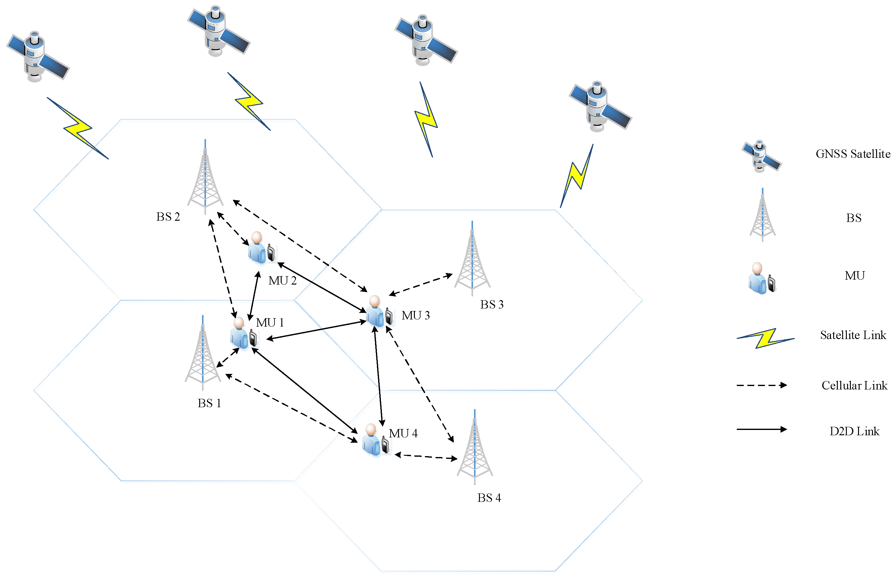
We consider a GNSS/5G integrated three-dimensional positioning system, as depicted in Figure 1, consisting of some GNSS satellites, $M$ BSs and $N$ MUs. The latter are denoted as $\mathcal{M}=\left\{1,2,\cdots ,M\right\}$ and $\mathcal{N}=\left\{1,2,\cdots ,N\right\}$, respectively. For convenience,

Table 1. Notation summary.

Symbol	Description
$\mathcal{M}=\left\{1,2,\cdots ,M\right\}$	Set of $M$ BSs
$\mathcal{N}=\left\{1,2,\cdots ,N\right\}$	Set of $N$ MUs
$\mathcal{N}\mathcal{R}=\left\{1,2,\cdots ,NR\right\}$	$\mathrm{Set} \mathrm{of} NR$ requesting nodes
$\mathcal{N}\mathcal{C}=\left\{1,2,\cdots ,NC\right\}$	$\mathrm{Set} \mathrm{of} NC$ cooperative nodes
$p_i=\left(x_i,y_i,z_i\right)$	The position of node $i$
$d_{ij}$	The distance between node $i$ and $j$
${\widehat{d}}_{ij}$	The estimated distance between node $i$ and $j$
$t_{0,ji}$$, t_{ij}$	The departure and arrival time of the signal from node $j$ to $i$, respectively
$\Delta t_{ij}$	The traveling time of the signal from node $j$ to $i$
$c$	Speed of light
$P{L}_{ij}^b$$, P{L}_{ij}^m$	The path loss of the signal between the BS and the MU and MUs, respectively
$f_c$	The carrier frequency of the transmitted signal
$S{F}_{ij}^b$	Shadow fading of the signal between the BS and the MU
${\alpha }_{ij}^b$$, {\alpha }_{ij}^m$	Flat fading coefficient of the signal between the BS and the MU and MUs, respectively
$s{t}_{ji}$$, s{r}_{ij}$	The transmitted and received signal from node $j$ to $i$, respectively
$\left(\epsilon ,MinPts\right)$	The size of the neighborhood and the minimum data points in a cluster, respectively
$Data=\left\{d{p}_1,d{p}_2,\cdots ,d{p}_n\right\}$	Data set of $n$ points in DBSCAN
$N_{\epsilon }\left(d{p}_i\right)$	$\epsilon -neighborhood$$\mathrm{of} d{p}_i$
${\mathcal{R}}_i$	The set of reference nodes of node $i$
$K_i=\left\{p{t}_1,\cdots ,p{t}_l,\cdots ,p{t}_{a_i}\right\}$	The set of positions calculated for node $i$
$P\left(X_k|Z_{1:k}\right)$	The posterior probability density at time slot $k$
$P{X}_k\left(f\right)$	The $f$th particle at time slot $k$
${\omega }_k\left(f\right)$	The weight of the $f$th particle at time slot $k$
$N_p$	The number of the particles

lists some important notations in this paper. We assume that the positions of the BSs are accurate. The MUs contain the requesting nodes that need positioning and the cooperative nodes with inaccurate known positions. Actually, the requesting nodes belong to cooperative nodes in cooperative positioning, while here we only name the MUs who serve as the reference nodes as the cooperative nodes, just to distinguish them. The requesting nodes and the cooperative nodes are denoted as $\mathcal{N}\mathcal{R}=\left\{1,2,\cdots ,NR\right\}$ and $\mathcal{N}\mathcal{C}=\left\{1,2,\cdots ,NC\right\}$, respectively. To be specific, each MU not only receives the positioning signals from the GNSS satellites, but is also capable of communicating with other MUs besides the BSs, known as D2D communication. The signals from the BSs and other MUs can also be used for positioning purpose. We assume that each D2D pair occupies one of the orthogonal frequency bands, and thus, there is no interference between these signals.

D2D communication enables two MUs in proximity to communicate directly without being relayed by a BS, which provides additional signal observations besides those from the BSs, and a meshed network structure rather than the traditional star shaped one can be obtained [18,19]. In this case, the requesting nodes can set up plenty of D2D links with other MUs, including the cooperative nodes and the other requesting nodes, to obtain pseudo ranges and share the position information and measurements. Actually, D2D positioning requires multi and frequent connection and a small amount of data, which is contrary to D2D communication. Meanwhile, a control link consuming much fewer resource is implemented for D2D discovery, link evaluation and resource allocation. Thus, to save link and time resource, an MU only exchanges the necessary data with other MUs via the D2D control links for positioning purposes [28].

As shown in Figure 1, each MU is connected to the BSs and some other MUs in proximity. If an MU is far from a BS, it may not be able to receive the signal from the BS. For example, the distance between BS 2 and MU 4 is too far to receive a qualified signal for MU 4 to position. Generally speaking, each MU needs four BSs for three-dimensional positioning without considering time synchronization in the wireless network. Here, the signals from the BSs and other close MUs can all be used for positioning.

2.2. Positioning Model in 5G

We assume that the BSs and the MUs are all equipped with GNSS chips, indicating that the time between them is synchronized. In the three-dimensional plane, there are two positioning methods for a requesting node: (i) the positioning signals from the GNSS satellites can be directly calculated to obtain the position, and (ii) the TOA and RSS measurements of four reference nodes (the BSs and the cooperative nodes), which can be transformed into the distances, are enough to be utilized for positioning if the MUs’ time offset is ignored. In practice, TOA-based positioning and RSS-based positioning are very popular due to their ready availability. To utilize the advantages of TOA and RSS measurements and improve the positioning accuracy, we exploited both of them to estimate the distances between the requesting nodes and the reference nodes, referred to as the joint TOA/RSS method.

In essence, the GNSS positioning and TOA- and RSS-based positioning supplemented with each other, which can be integrated to obtain a more accurate solution, and we illustrate the integrated method in the next subsection. Here, we mainly focus on the distance estimation based on TOA and RSS measurements. In the following, the distance-based positioning is described firstly, and then, TOA and RSS measurements are analyzed in detail to estimate the distances between the nodes, respectively.

2.2.1. Distance Based Positioning

Without loss of generality, the BSs and the MUs are all seen as the nodes which can function as reference nodes; $\left(x_i,y_i,z_i\right)$ and $\left(x_j,y_j,z_j\right)$ are the positions of node $i$ and $j$, respectively. For a requesting node $i$ and a reference node $j$, the distance between them can be represented as

$$d_{ij}=\sqrt{{\left(x_i-x_j\right)}^2+{\left(y_i-y_j\right)}^2+{\left(z_i-z_j\right)}^2}$$

(1)

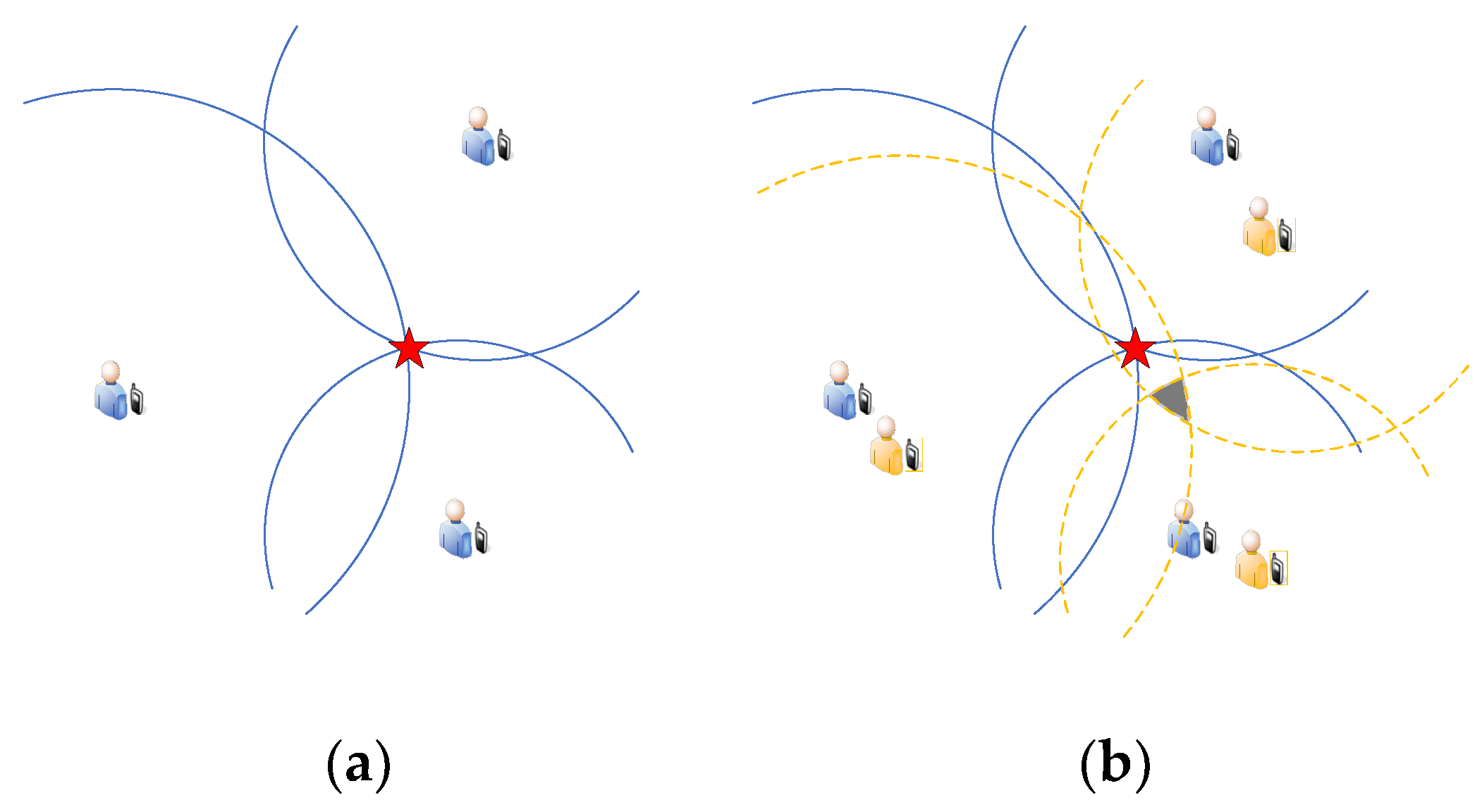
Intuitively, Figure 2a illustrates the two-dimensional positioning procedure based on trilateration when there are three reference nodes. The red star represents the true position of a requesting node. When the TOA or the RSS measurements between the requesting node and the reference nodes are known, the distances between them can be obtained. Regardless of the error in distance measurements, the three blue curves shown in Figure 2a intersect in a red star. By analogy, four reference nodes are needed for a requesting node to decide its three-dimensional position and for four spheres to meet at one point.

2.2.2. TOA-Based Distance Estimation

The distance between two nodes depends on the traveling time and the traveling speed of the signal transmitted from one node to the other. Here, we assume that a timestamp $t_{0,ji}$ is attached to the signal from node $j$ to node $i$ before node $j$ transmits it, i.e., the departure time of the signal can be obtained. The arrival time at node $i$ is shown as

$$t_{ij}=t_{0,ji}+\frac{d_{ij}}{c}+{\delta }_{ij}$$

(2)

where $d_{ij}$ is the true distance between node $i$ and $j$, and ${\delta }_{ij}$ is a zero-mean random variable with a variance of ${\sigma }_t^2$, which is caused by the measurement error. To be general, we assume that ${\sigma }_t^2$ for different nodes is the same and obeys the Gaussian distribution [23]. Besides, the signal travels at the speed of light, which is denoted as $c$. Denote $\Delta t_{ij}$ as the traveling time of the positioning signal between node $i$ and $j$ with error ${\delta }_{ij}$ based on the above analysis. Then, we have

$$\Delta t_{ij}=t_{ij}-t_{0,ji}=\frac{d_{ij}}{c}+{\delta }_{ij}$$

(3)

$$\Delta t_{ij}\sim \mathcal{N}\left(\frac{d_{ij}}{c},{\sigma }_t{}^2\right)$$

(4)

According to the above analysis, the estimated distance between node $i$ and $j$ is expressed as

$$\begin{array}{ll}{\widehat{d}}_{ij}& =c\Delta t_{ij} \\ & =c\left(\frac{d_{ij}}{c}+{\delta }_{ij}\right)\\ & =d_{ij}+c{\delta }_{ij} \end{array}$$

(5)

Obviously, the estimated distance between node $i$ and $j$ consists of the true distance between the two nodes and an additional error from the measurement error.

2.2.3. RSS-Based Distance Estimation

In general, if the signal propagation model is determined, and the transmitted signal at one node and the received signal at the other node are known, the distance between these two nodes can be obtained. In the following, we firstly illustrate the three-dimensional signal propagation model based on our system model, and then, the distance estimation based on the RSS measurements is given.

• Signal Propagation between the BS and the MU

We apply the typical urban macro cell three-dimensional channel model proposed in the 3rd Generation Partnership Project (3GPP) for the signal propagation between the BS and the MU [31]. Generally, a small-scale fading effect mainly originates from the multipath effect, which can be ignored due to our requirements of the received signals. In this regard, we focus on the large-scale fading parameters. If the requesting node is denoted as node $i$, then the BS as $j$. The path loss of the signal between node $i$ and $j$ is represented as:

$$P{L}_{ij}^b\left[\mathrm{dB}\right]=A\log \left(d_{ij}\left[\mathrm{m}\right]\right)+B+C\log \left(f_c\left[\mathrm{GHz}\right]\right)$$

(6)

where $f_c$ is the carrier frequency of the transmitted signal. Specifically, only the signal with line-of-signal (LoS) reception is considered to guarantee the quality of service (QoS), which means that the distance between the nodes capable of positioning is within a threshold.

In addition to the large-scale fading, shadow fading also needs to be taken into account. It is a random process drawn in dB from a normal distribution with zero mean and a variance of ${\sigma }_{SF}^2$ [19], expressed as:

$$S{F}_{ij}^b\left[\mathrm{dB}\right]=\mathcal{N}\left(0,{\sigma }_{SF}^2\right)$$

(7)

According to the above analysis, the large-scale fading and shadow fading can be integrated into the flat fading coefficient ${\alpha }_{ij}^b$, reflecting the overall path loss of the signal:

$${\alpha }_{ij}^b={10}^{-\frac{P{L}_{ij}^b+S{F}_{ij}^b}{20}}$$

(8)

• Signal Propagation between the MUs

Contrary to the signal propagation between the BS and the MU, the free space path loss without shadow fading is considered for the propagation between the MUs. Then, we would have [19]

$$P{L}_{ij}^m\left[\mathrm{dB}\right]=20\log \left(d_{ij}\left[\mathrm{m}\right]\right)+32.4+20\log \left(f_c\left[\mathrm{GHz}\right]\right)$$

(9)

for the free space path loss between node $i$ and $j$. Accordingly, the flat fading coefficient is shown as:

$${\alpha }_{ij}^m={10}^{-\frac{P{L}_{ij}^m}{20}}$$

(10)

• Distance Estimation

If node $j$ transmits a signal $s{t}_{ji}$ to node $i$, the received signal at node $i$ is as follows:

$$s{r}_{ij}={\alpha }_{ij}s{t}_{ji}+n_{ij}$$

(11)

where ${\alpha }_{ij}={\alpha }_{ij}^b$ or ${\alpha }_{ij}={\alpha }_{ij}^m$ is the flat fading coefficient when node $j$ is a BS or an MU, respectively. $n_{ij}$ is the additive white Gaussian noise, which can be expressed as:

$$n_{ij}\sim \mathcal{N}\left(0,{\sigma }_r^2\right)$$

(12)

where ${\sigma }_r^2$ is the variance of the Gaussian distribution. Similarly, ${\sigma }_r^2={\sigma }_{r,b}^2$ or ${\sigma }_r^2={\sigma }_{r,m}^2$ is the variance for the BS or the MU, respectively.

Since both the transmitted signal $s{t}_{ji}$ and the received signal $s{r}_{ij}$ are obtained, we can calculate the flat fading coefficient, which can be further used to estimate the distance between the two nodes based on (6) or (9). Nevertheless, it has to be pointed out that the estimated distance is not an accurate one because of various noises.

2.3. GNSS/5G Integrated Three-Dimensional Positioning Scheme

In this subsection, we propose a GNSS/5G integrated three-dimensional positioning scheme. As Figure 2b indicates, an area bounded by three intersecting circles is represented by a shade of gray in the two-dimensional positioning, when the positions of the reference nodes are inaccurate. Similarly, a stereo region will be formed in the three-dimensional positioning. As earlier mentioned, the positions of the cooperative nodes are not accurate enough to act as the reference nodes, and then, the positioning results of the requesting nodes will be affected. If we choose four reference nodes to position a requesting node each time, there will be a lot of position results with some errors. DBSCAN can keep the high-density data points and remove the outliers in the sample data set. Then, the outlying results with large errors can be identified when a large number of calculated positions of a node are available. Thus, according to the GNSS and TOA/RSS measurements, we firstly exploit DBSCAN to obtain relatively accurate positions of the requesting nodes. Meanwhile, we can also reduce the position deviation of the cooperative nodes. Then, the results from the DBSCAN algorithm are input as the initial state of the MUs in PF, which further integrate with the TOA/RSS measurements.

2.3.1. GNSS/5G Integrated Three-Dimensional Positioning Based on DBSCAN

Firstly, we describe DBSCAN briefly. Then, the GNSS/5G integrated three-dimensional positioning algorithm exploiting the joint TOA/RSS method is proposed.

• DBSCAN

Clustering classifies the data set into different groups according to a standard of association. As a result, the data points in the same cluster are similar, while the data points in different clusters are not. The input of the clustering is a sample data set and a standard of similarity between two points, and the output is some partitions of the sample data set without intersection [32].

DBSCAN is a density-based clustering, which assumes that the clusters can be determined by the density of the data set [33]. To be specific, the clusters are the collections of data points with high density separated by the regions of low data point density. That is, the density of the data points within a cluster is considerably higher than those outside of the cluster.

We denoted $\left(\epsilon ,MinPts\right)$ as the neighborhood parameters to depict the closeness of the data point distribution, which reflects the size of the neighborhood and the minimum data points in a cluster, respectively. Here, for an arbitrary data point $d{p}_i$, $\epsilon -neighborhood$ is defined as:

$$N_{\epsilon }\left(d{p}_i\right)=\left\{d{p}_j\in Data|dist\left(d{p}_i,d{p}_j\right)\le \epsilon \right\}$$

(13)

where $Data=\left(d{p}_1,d{p}_2,\cdots ,d{p}_n\right)$ is the data set, and $dist(\cdot )$ represents the distance between two data points. $N_{\epsilon }\left(d{p}_i\right)$ denotes the data points at a distance from $d{p}_i$ shorter than $\epsilon$. If the $\epsilon -neighborhood$ of data point $d{p}_i$ exceeds $MinPts$, i.e., $\left|N_{\epsilon }\left(d{p}_i\right)\right|\ge MinPts$, $d{p}_i$ is called a core object.

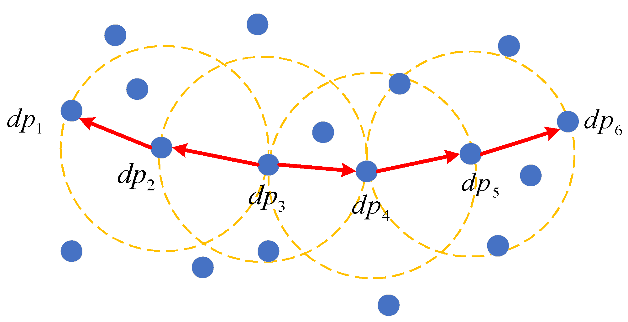
According to [34], some definitions can be given intuitively in Figure 3. The yellow dashed lines and the blue solid points represent the $\epsilon -neighborhood$ and the data points, respectively. Assume that $d{p}_3$ is a core object, and then, $d{p}_2$ and $d{p}_1$ are directly density-reachable and density-reachable from $d{p}_3$, respectively, as shown in Figure 3. In addition, $d{p}_1$ and $d{p}_6$ are density-connected. The key idea of DBSCAN is that, for a given size of neighborhood $\epsilon$, each formed cluster contains as many as density-connected data points, the amount of which is at least $MinPts$ [32].

• GNSS/5G Integrated Three-Dimensional Positioning Algorithm Based on DBSCAN

At first, we exploit the GNSS measurements to calculate the initial positions for the requesting nodes. As we all know, the GNSS positioning is in the accuracy of several meters in the kinematic situation. In addition, the cooperative nodes only know their inaccurate positions. In other words, the known position of each MU in the network is not accurate. However, more accurate positions of the cooperative nodes further used in the following algorithm can improve the position accuracy of the requesting nodes. Hence, we also take into account the prior information of the cooperative nodes in the clustering process to obtain more accurate positions of them, i.e., the cooperative nodes are also regarded as the requesting nodes, and then, the BSs and other MUs are seen as the reference nodes. According to this, the positions of the requesting nodes and the cooperative nodes, i.e., the positions of the MUs, are all in need of revision in the DBSCAN algorithm.

For each MU, there are $M$ BSs and $N-1$ other MUs potential for positioning. Actually, not all of these potential nodes can finally be the reference nodes. According to the analysis in Section 2.2, the distance between the reference nodes and the requesting node should be short enough to guarantee the QoS, otherwise they cannot be taken into account as the reference nodes. Here, the requesting nodes and the cooperative nodes share the potential reference nodes in the same set of the MUs in addition to the BSs. Besides, as the cooperative nodes and the requesting nodes are ordinary MUs in the network, the positioning method and the signal propagation model for them are the same.

Without loss of generality, we firstly focus on MU $i$ to illustrate the generation of the sample data set before implementing the clustering process. We denote $p_i=\left(x_i,y_i,z_i\right)$ as the initial position of MU $i$, which is inaccurate. The set of the initial positions of all the MUs in the network is $\mathcal{P}\mathcal{I}=\left\{p_1,\cdots ,p_i,\cdots ,p_N\right\}$. Assume that the nodes, including the BSs and other MUs from which the distance to MU $i$ is within $MaxD$, are the reference nodes of MU $i$, i.e., ${\mathcal{R}}_i=\left\{j\in \mathcal{M}\cup \mathcal{N},j\ne i|d_{ij}\le MaxD\right\}$. Then, $\left|{\mathcal{R}}_i\right|$ represents the number of the reference nodes. As any four reference nodes in ${\mathcal{R}}_i$ can determine the only position of MU $i$, there are $a_i=C_{\left|{\mathcal{R}}_i\right|}^4$ positions obtained, which further form the data points in the clustering. These positions are shown as:

$${\mathcal{K}}_i=\left\{p{t}_1,\cdots ,p{t}_l,\cdots ,p{t}_{a_i}\right\}$$

(14)

where $p{t}_l$ is the position calculated through the $l$th combination of the reference nodes. The data points in the clustering are composed of the calculated positions of $N$ MUs in the network, and accordingly, the data points are shown as $\mathcal{K}=\left\{{\mathcal{K}}_1,\cdots ,{\mathcal{K}}_i,\cdots ,{\mathcal{K}}_N\right\}$.

Here, we exploit both TOA and RSS measurements to calculate the distance between two nodes, which is probably different. Consequently, the obtained positionsare different. We firstly implement two independent clustering process using TOA and RSS measurements, respectively, and then they are integrated through a weighting method. It is obvious that ${\mathcal{R}}_i$ and ${\mathcal{K}}_i$ for MU $i$ are different in these two methods. Hence, as for MU $i$, we denote ${\mathcal{R}}_{t,i}=\left\{j\in \mathcal{M}\cup \mathcal{N},j\ne i|d_{t,ij}\le MaxD\right\}$ and ${\mathcal{K}}_{t,i}=\left\{p{t}_{t,1},\cdots ,p{t}_{t,l},\cdots ,p{t}_{t,a_{t,i}}\right\}$ for the TOA measurements, and we denote ${\mathcal{R}}_{r,i}=\left\{j\in \mathcal{M}\cup \mathcal{N},j\ne i|d_{r,ij}\le MaxD\right\}$ and ${\mathcal{K}}_{r,i}=\left\{p{t}_{r,1},\cdots ,p{t}_{r,l},\cdots ,p{t}_{r,a_{r,i}}\right\}$ for the RSS measurements. $a_{t,i}=C_{\left|{\mathcal{R}}_{t,i}\right|}^4$ and $a_{r,i}=C_{\left|{\mathcal{R}}_{r,i}\right|}^4$ are the numbers of calculated positions for MU $i$ based on the TOA and RSS measurements, respectively. As a result, the set of the data points in the clustering are ${\mathcal{K}}^t=\left\{{\mathcal{K}}_{t,1},\cdots ,{\mathcal{K}}_{t,i},\cdots ,{\mathcal{K}}_{t,N}\right\}$ and ${\mathcal{K}}^r=\left\{{\mathcal{K}}_{r,1},\cdots ,{\mathcal{K}}_{r,i},\cdots ,{\mathcal{K}}_{r,N}\right\}$ for the two kinds of measurements, and the numbers of the data points are denoted as $DataNu{m}^t$ and $DataNu{m}^r$, respectively.

Then, the DBSCAN algorithm is implemented based on the TOA and RSS measurements separately. We take the TOA measurements, for example, and the clustering process based on the RSS measurements is the same. We summarize the DBSCAN based on the TOA measurements in Algorithm 1 as DATM. For further explanation, there are two main steps. Firstly, the positions calculated by the TOA measurements are regarded as the data points in the clustering, and we find the core objects according to $\left(\epsilon ,MinPts\right)$, as lines 2 to 7 show. Then, the clusters are formed according to the density of the data points, in which each cluster gather around the position of an MU, as line 8 to 19 indicate.

The DBSCAN algorithm based on the RSS measurements is similar to DATM. After obtaining the clustering results based on both of the measurements, the results are weighted according to their variance. We also take the clustering result based on the TOA measurements, for example, and the weighting process is as follows. As mentioned in DATM, $p_{t,h}=\left(x_{t,h},y_{t,h},z_{t,h}\right)$ is the mean value of the $h$th cluster, which indicate the position of an MU. We assumed that there are $b_h$ data points in the $h$th cluster denoted as $\mathcal{C}{\mathcal{K}}_{t,h}=\left\{p{c}_{t,1},\cdots ,p{c}_{t,g},\cdots ,p{c}_{t,b_h}\right\}$, where $p{c}_{t,g}=\left(x{c}_{t,g},y{c}_{t,g},z{c}_{t,g}\right)$. Then, the variance of the east, north and up coordinate in the $h$th cluster is shown respectively as

$$v{x}_{t,h}={\displaystyle \sum _{g=1}^{b_h}{\left(x_{t,h}-x{c}_{t,g}\right)}^2}$$

(15)

$$v{y}_{t,h}={\displaystyle \sum _{g=1}^{b_h}{\left(y_{t,h}-y{c}_{t,g}\right)}^2}$$

(16)

$$v{z}_{t,h}={\displaystyle \sum _{g=1}^{b_h}{\left(z_{t,h}-z{c}_{t,g}\right)}^2}$$

(17)

Accordingly, we can obtain $v{x}_{r,h}$, $v{y}_{r,h}$ and $v{z}_{r,h}$ for the $h$th cluster based on the RSS measurements. Since the distribution in the east, north and up coordinate may be different, we integrate the clustering results in different coordinates, respectively. Then, we define the position based on the joint TOA/RSS method as $p_{tr,h}=\left(x_{tr,h},y_{tr,h},z_{tr,h}\right)$, where $x_{tr,h}$, $y_{tr,h}$ and $z_{tr,h}$ are respectively represented as [35]

$$x_{tr,h}=\frac{\frac{1}{\sqrt{v{x}_{t,h}}}}{\frac{1}{\sqrt{v{x}_{t,h}}}+\frac{1}{\sqrt{v{x}_{r,h}}}}{x}_{t,h}+\frac{\frac{1}{\sqrt{v{x}_{r,h}}}}{\frac{1}{\sqrt{v{x}_{t,h}}}+\frac{1}{\sqrt{v{x}_{r,h}}}}{x}_{r,h}$$

(18)

$$y_{tr,h}=\frac{\frac{1}{\sqrt{v{y}_{t,h}}}}{\frac{1}{\sqrt{v{y}_{t,h}}}+\frac{1}{\sqrt{v{y}_{r,h}}}}{y}_{t,h}+\frac{\frac{1}{\sqrt{v{y}_{r,h}}}}{\frac{1}{\sqrt{v{y}_{t,h}}}+\frac{1}{\sqrt{v{y}_{r,h}}}}{y}_{r,h}$$

(19)

$$z_{tr,h}=\frac{\frac{1}{\sqrt{v{z}_{t,h}}}}{\frac{1}{\sqrt{v{z}_{t,h}}}+\frac{1}{\sqrt{v{z}_{r,h}}}}{z}_{t,h}+\frac{\frac{1}{\sqrt{v{z}_{r,h}}}}{\frac{1}{\sqrt{v{z}_{t,h}}}+\frac{1}{\sqrt{v{z}_{r,h}}}}{z}_{r,h}$$

(20)

Here, we obtain the positions based on the joint TOA/RSS method after the DBSCAN algorithm, represented as ${\mathcal{P}}_{tr}=\left\{p_{tr,1},p_{tr,2},\cdots ,p_{tr,u}\right\}$.

Algorithm 1: DBSCAN Algorithm Based on The TOA Measurements (DATM)

Input: ${\mathcal{K}}^t=\left\{{\mathcal{K}}_{t,1},\cdots ,{\mathcal{K}}_{t,i},\cdots ,{\mathcal{K}}_{t,N}\right\}$, $\left(\epsilon ,MinPts\right)$ 1: Initialization: Let $\mathsf{\Omega }=\varnothing$ be the set of core objects, $u=0$ be the number of clusters and $\Gamma ={\mathcal{K}}^t$ be the sample data set unvisited 2: for all $r\in {\mathcal{K}}^t$ do 3:  determine the $\epsilon -neighborhood$ of data point $d{p}_r$ as $N_{\epsilon }\left(d{p}_r\right)=\left\{d{p}_s\in {\mathcal{K}}^t|dist\left(d{p}_r,d{p}_s\right)\le \epsilon \right\}$ defined in (13) 4:  if $\left|N_{\epsilon }\left(d{p}_r\right)\right|\ge MinPts$ then 5:  $d{p}_r$ is added to the set of the core objects: $\mathsf{\Omega }=\mathsf{\Omega }\cup \left\{d{p}_r\right\}$ 6: end 7: end 8: while $\mathsf{\Omega }=\varnothing$ do 9:  set the current unvisited sample data set as ${\Gamma }_{old}=\Gamma$, select a core object $o\in \mathsf{\Omega }$ and    denote a queue as $Q=\langle o\rangle$, then $\Gamma =\Gamma \backslash \left\{o\right\}$ 10:  while $Q\ne \varnothing$ do 11:   extract the first data point $q$ in $Q$ 12:   if $\left|N_{\epsilon }\left(q\right)\right|\ge MinPts$ then 13:    $\Delta =N_{\epsilon }\left(q\right)\cap \Gamma$ and add the data points in $\Delta$ to $Q$, $\Gamma =\Gamma \backslash \Delta$ 14:   end 15:  end 16:  $u=u+1$ and the formed cluster is $C_{t,u}={\Gamma }_{old}\backslash \Gamma$ 17:  $\mathsf{\Omega }=\mathsf{\Omega }\backslash C_{t,u}$ 18: end 19: Output the clustering result ${\mathcal{C}}^t=\left\{C_{t,1},C_{t,2},\cdots ,C_{t,u}\right\}$ and calculate the mean value of each cluster in ${\mathcal{C}}^t$ denoted as $\mathcal{P}{\mathcal{C}}^t=\left\{p_{t,1},p_{t,2},\cdots ,p_{t,u}\right\}$

2.3.2. GNSS/5G Integrated Three-Dimensional Positioning Based on PF

PF is appropriate for the heterogeneous positioning methods with various noise, which forms a non-linear problem. Hence, based on the positions obtained from the DBSCAN algorithm, we further exploit PF to improve the accuracy of the positions of the requesting nodes. We firstly describe the concept of PF, and then, the GNSS/5G integrated three-dimensional positioning algorithm based on PF is proposed.

• PF

PF is a probability-based estimator, which originates from the sequential Monte Carlo estimation method [36]. The main idea of PF is that the probability density is described in terms of the random samples, known as the particles, together with their corresponding normalized weights. PF is well suited to the nonlinear problems with respect to state-transition models and observation models, since the sample-based method can describe the general probability density [37].

The purpose of filtering is to recursively estimate the posterior probability density $P\left(X_k|Z_{1:k}\right)$ at time slot $k$, which is approximated by a set of particles and the corresponding normalized weights in the form

$$P\left(X_k|Z_{1:k}\right)\approx {\displaystyle \sum _{f=1}^{N_p}{\omega }_k\left(f\right)\delta \left(X_k-P{X}_k\left(f\right)\right)}$$

(21)

where $X_k$ is the state, and $Z_{1:k}$ is the observation. $P{X}_k\left(f\right)$ is the $f$th particle, and ${\omega }_k\left(f\right)$ is the corresponding normalized weight. $\delta (·)$ is the Dirac delta function. $N_p$ is the total number of particles. Here, the sequential importance sampling (SIS) is exploited. Indeed, it is difficult to sample the posterior probability density $P\left(X_k|Z_{1:k}\right)$. According to the SIS, a known distribution $q\left(X_k|Z_{1:k}\right)$ called importance distribution is introduced for sampling which approximates $P\left(X_k|Z_{1:k}\right)$. Besides, the SIS can realize the recursive estimation of the weights. Then, based on the sequential Bayes theory, we have [38]

$$P\left(X_{1:k}|Z_{1:k}\right)=\frac{P\left(Z_k|X_k\right)P\left(X_k|X_{k-1}\right)}{P\left(Z_k|Z_{1:k-1}\right)}P\left(X_{1:k-1}|Z_{1:k-1}\right)$$

(22)

and the importance distribution is shown as

$$q\left(X_{1:k}|Z_{1:k}\right)=q\left(X_k|X_{1:k-1},Z_{1:k}\right)q\left(X_{1:k-1}|Z_{1:k-1}\right)$$

(23)

Thus, the weights of the particles are obtained:

$${\omega }_k\left(f\right)=\frac{P\left(X_{1;k}|Z_{1:k}\right)}{q\left(X_{1:k}|Z_{1:k}\right)}\propto \frac{P\left(Z_k|X_k\right)P\left(X_k{|X}_{k-1}\right)}{q\left(X_k|X_{1:k-1},Z_{1:k}\right)}{\omega }_{k-1}\left(f\right)$$

(24)

For simplicity, $q\left(X_k|X_{1:k-1},Z_{1:k}\right)=P\left(X_k|X_{k-1}\right)$ is chosen in the SIS. Thus, (24) is written as:

$${\omega }_k\left(f\right)\propto P\left(Z_k|X_k\right){\omega }_{k-1}\left(f\right)$$

(25)

Nevertheless, the variation among the weights will increase with the time, which is the particle degeneracy phenomenon. After several recursions, the weights of most particles tend to be 0 while the remaining tend to be 1. It means that most of the sample points have to be discarded. To avoid this phenomenon, we adopt resampling to sample the high weight particles repeatedly and delete the low weight particles. In essence, the resampling maps the original particles into the updated particles distributed uniformly. In other words, the weight of each updated particle is equal, i.e., $\frac{1}{N_p}$. Therefore, the state estimation after the resampling is

$${\widehat{X}}_k=\frac{1}{N_p}{\displaystyle {\displaystyle \sum }_{f=1}^{N_p}P{X}_k\left(f\right)}$$

(26)

• GNSS/5G Integrated Three-Dimensional Positioning Algorithm Based on PF

Here, we consider the requesting nodes in $\mathcal{N}\mathcal{R}$. The BS in $\mathcal{M}$ and the cooperative nodes in $\mathcal{N}\mathcal{C}$ are the potential reference nodes. In practice, the reference nodes are not all visible to the requesting nodes as mentioned above. Without loss of generality, we concentrate on MU $i$ in $\mathcal{N}\mathcal{R}$. According to the distance constraint, the visible reference nodes constitute a set denoted as ${\mathcal{R}}^i$. We denote $\psi =\left\{t,r\right\}$ as the TOA and RSS measurements, where $t$ represents the TOA measurements, and $r$ represents the other. $k$ is the time when the DBSCAN algorithm based on the joint TOA/RSS method outputs. We assume that at time $k$, the requesting nodes not only know their own positions from the DBSCAN results, but also the positions of the BSs and the cooperative nodes. In addition, the GNSS and TOA/RSS measurements are available at time $k$.

PF is implemented for each MU in $\mathcal{N}\mathcal{R}$. Here, for MU $i$, in addition to the BSs that can be used for positioning, denoted as ${\mathcal{M}}_{tr}$, the reference nodes based on the TOA and RSS measurements form ${\mathcal{R}}_{t,i}$ and ${\mathcal{R}}_{r,i}$, respectively. The objective is to find the state of MU $i$ denoted as $X_k^i$, which maximizes the posterior distribution, formulated as follows:

$$\max bel\left(X_k^i\right)=P\left(X_k^i|{\mathcal{I}}_{1:k}^{i{N}^{i^2}}\right)\hspace{1em}\forall i\in \mathcal{N}\mathcal{R}$$

(27)

where ${\mathcal{N}}^{i^2}={\mathcal{R}}_{t,i}\cup {\mathcal{R}}_{r,i}\cup {\mathcal{M}}_{tr}\cup i$, and we denote ${\mathcal{N}}^i={\mathcal{R}}_{t,i}\cup {\mathcal{R}}_{r,i}\cup {\mathcal{M}}_{tr}$. Then, $i{\mathcal{N}}^{i^2}$ includes $ii$ and all the $ij$s where $j\in {\mathcal{N}}^i$. ${\mathcal{I}}_{1:k}^{i{\mathcal{N}}^{i^2}}$ represents the collected information before time $k$. ${\mathcal{I}}_k^{ii}$ contains $Z_{D,k}^{tr,i{\mathcal{N}}^i}$, the TOA and RSS measurements between MU $i$ and all the $j$s in ${\mathcal{N}}^i$. ${\mathcal{I}}_k^{i{\mathcal{N}}^i}$ contains the estimated state of all the $j$s in ${\mathcal{N}}^i$ at time $k-1$, denoted as ${\widehat{X}}_{k-1}^j$. Then, based on the initial position obtained from the DBSCAN output, $X_k^i$ in (27) is the integrated position of MU $i$. Besides, (27) can be further expressed in (28) based on the Bayesian formula:

$$\begin{array}{l}P\left(X_k^i|{\mathcal{I}}_{1:k}^{i{\mathcal{N}}^{i^2}}\right)={\displaystyle {\displaystyle \int }P\left(X_k^{{\mathcal{N}}^{i^2}}|{\mathcal{I}}_{1:k}^{i{\mathcal{N}}^{i^2}}\right)}\partial X_k^{{\mathcal{N}}^i}\\ \propto {\displaystyle {\displaystyle \int }P\left(Z_{D,k}^{tr,i{\mathcal{N}}^i}{\widehat{X}}_{k-1}^{{\mathcal{N}}^i}|X_k^{{\mathcal{N}}^{i^2}}\right)}P\left(X_k^{{\mathcal{N}}^{i^2}}|X_{k-1}^{{\mathcal{N}}^{i^2}}\right)P\left(X_{k-1}^i|{\mathcal{I}}_{1:k-1}^{i{\mathcal{N}}^{i^2}}\right)\partial X_k^{{\mathcal{N}}^i}\end{array}$$

(28)

From Equation (28), it is obvious that the first two items are the likelihood function and the prediction function, which represent the weights of the particles and the importance distribution, respectively. Then, the GNSS/5G integrated three-dimensional positioning algorithm based on PF is illustrated in Algorithm 2 as GITPAPF. Firstly, as shown in line 1, we initialize the particles based on the DBSCAN output and the important distribution. After that, in each time slot, we use PF to estimate the state of $X_k^i$, as line 2 to 9 indicate. For each requesting node in $\mathcal{N}\mathcal{R}$, GITPAPF is conducted to obtain the integrated position result.

Notice that the size of ${\mathcal{N}}^{i^2}$ determines the size of $X_k^{{\mathcal{N}}^{i^2}}$, and a large number of particles have to be sampled and calculated to obtain the integrated positions of the requesting nodes in $\mathcal{N}\mathcal{R}$. Hence, the edge computing is exploited to overcome the problem of limited computing resources in the MUs, which can also shorten the delay of positioning.

Algorithm 2: GNSS/5G Integrated Three-Dimensional Positioning Algorithm Based on Particle Filter (GITPAPF)

Input: the initial distribution $p\left(X_0^{{\mathcal{N}}^{i^2}}\right)$ 1: Initialization: generate the initial state of the particles $P{X}_0^{{\mathcal{N}}^{i^2}}\left(f\right)\left(f=1,2,\cdots ,N_p\right)$ according to $P\left(X_0^{{\mathcal{N}}^{i^2}}\right)$ 2: for all $k=1,2,3,\cdots$ do 3:  let $q\left(X_k^{{\mathcal{N}}^{i^2}}|X_{k-1}^{{\mathcal{N}}^{i^2}}\right)=P\left(X_k^{N^{i^2}}|X_{k-1}^{N^{i^2}}\right)$ be the importance distribution 4:  sample the particles at time slot $k$ according to $P{X}_k^{{\mathcal{N}}^{i^2}}\left(f\right)\sim q\left(X_k^{{\mathcal{N}}^{i^2}}|X_{k-1}^{{\mathcal{N}}^{i^2}}\right)$ 5:  calculate the weights of the particles at time slot $k$:   ${\omega }_k^{{\mathcal{N}}^{i^2}}\left(f\right)\propto P\left(Z_{D,k}^{tr,i{\mathcal{N}}^i},{\widehat{X}}_{k-1}^{{\mathcal{N}}^i}|X_k^{{\mathcal{N}}^{i^2}}\right)$ 6:  normalize the weights: ${\tilde{\omega }}_k^{{\mathcal{N}}^{i^2}}\left(f\right)={\omega }_k^{{\mathcal{N}}^{i^2}}\left(f\right){\left[{\displaystyle \sum _{f=1}^{N_p}{\omega }_k^{{\mathcal{N}}^{i^2}}\left(f\right)}\right]}^{-1}$ 7: resampling the particles and the weight of each of them is $\frac{1}{N_p}$ 8: calculate the estimated state at time slot $k$ as ${\widehat{X}}_k^i=\frac{1}{N_p}{\displaystyle \sum _{f=1}^{N_p}P{X}_k^i\left(f\right)}$ and output the result 9: end

2.3.3. GNSS/5G Integrated Three-Dimensional Positioning Algorithm

Based on the above analysis, the GNSS/5G integrated three-dimensional positioning algorithm is summarized in Algorithm 3 as GITPA. Specifically, there are three steps. Firstly, based on the GNSS and TOA/RSS measurements, we obtain the positions of all the MUs according to DATM, including the requesting nodes and the cooperative nodes, as shown in lines 1 and 2. Then, the clustering results based on the TOA and RSS measurements are weighted, as lines 3 to 7 indicate. In final, GITPAPF is conducted to further improve the accuracy of the requesting nodes, as line 8 indicates.

Algorithm 3: GNSS/5G Integrated Three-Dimensional Positioning Algorithm (GITPA)

Input: $\mathcal{P}\mathcal{I}$ 1: generate the data points for DATM based on $\mathcal{P}\mathcal{I}$ and the TOA/RSS measurements 2: conduct DATM according to the TOA and RSS measurements respectively, and each pair of the closest clusters based on both of the measurements are given the same number 3: for all $h=1,2,\cdots ,u$ do 4:   calculate $v{x}_{t,h}$, $v{x}_{r,h}$, $v{y}_{t,h}$, $v{y}_{r,h}$, $v{z}_{t,h}$ and $v{z}_{r,h}$ according to (15), (16) and (17), respectively 5:    obtain $p_{tr,h}=\left(x_{tr,h},y_{tr,h},z_{tr,h}\right)$ according to (18), (19) and (20) 6: end 7: let ${\mathcal{P}}_{tr}=\left\{p_{tr,1},p_{tr,2},\cdots ,p_{tr,u}\right\}$ 8: project ${\mathcal{P}}_{tr}$ into ${\mathcal{I}}_0^{i{\mathcal{N}}^{i^2}}$ and conduct GITPAPF for each MU in $\mathcal{N}\mathcal{R}$

3. Results

In this section, we carry out several numerical simulations to evaluate the proposed algorithm. The simulation setup is as follows. Consider an urban cellular mobile radio environment with four BSs and 13 MUs, and the latter is composed of five requesting nodes and eight cooperative nodes. Meanwhile, GNSS satellites are available to provide the measurements for the MUs. We assume a default height of the BSs, denoted as $h_{BS}=25 \mathrm{m}$, and the height of the MUs satisfies $1.5 \mathrm{m}\le h_{MU}\le 22.5 \mathrm{m}$. Hence, according to [31], the signal propagation model parameters for the propagation between the BS and the MUs can be obtained, i.e., $A=22$, $B=28$, $C=20$ and ${\sigma }_{SF}^2=4 \mathrm{dB}$. In general, as the transmitting distance between two D2D users is below 100 m, to guarantee the QoS between the requesting nodes and the reference nodes to obtain reliable range measurements, we set the maximum distance between them as 50 m; ${\sigma }_t^2={10}^{-10}$ is set for the TOA measurements [39], and ${\sigma }_{r,b}^2=4\times {10}^{-14}$ and ${\sigma }_{r,m}^2={10}^{-14}$ are set for the RSS measurements [19]. In the DBSCAN process, the neighborhood parameters are $\epsilon =0.5$ and $MinPts=10$. In fact, to achieve time synchronization in GNSS/5G integrated positioning, a one-way system proposed in [15] is exploited to provide a unified time system, and the ionospheric and tropospheric effect in GNSS can be significantly corrected according to the ephemeris of the satellites.

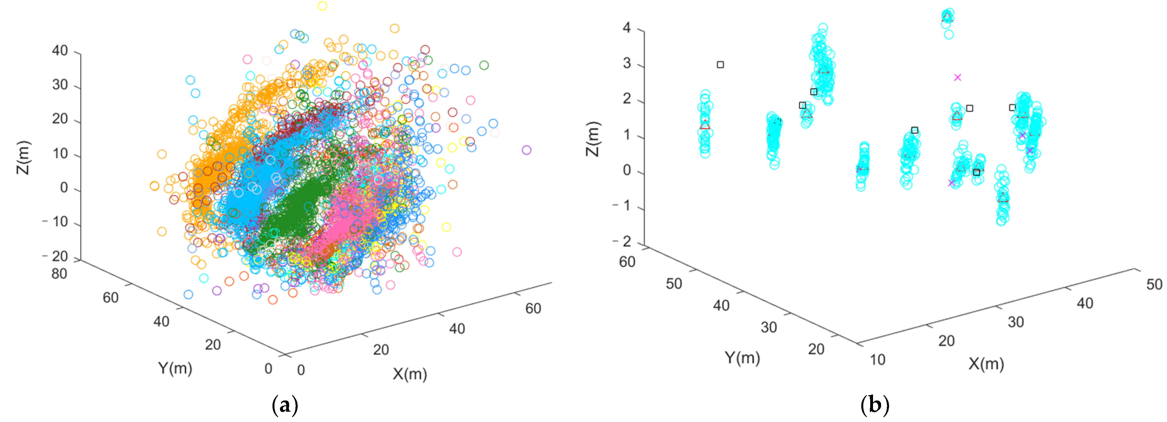
Firstly, Figure 4 gives an intuitional impression of the effect of the DBSCAN, which shows the distribution of the data points before and after the DBSCAN process. Actually, those data points represent the calculated positions of the MUs based on the TOA measurements. As the result based on the RSS measurements is similar to Figure 4, it was omitted due to limited space. There are 13 MUs in the simulation, including five requesting nodes and eight cooperative nodes. An amount of 100 particles are used in the PF process. In Figure 4a, the calculated positions of each MU are represented by a single color, and we can see that some data points concentrate on a center and others are scattered. After the DBSCAN process, as Figure 4b shows, those scattered data points are all removed as outliers and the clusters are formed, where the cyan circles represent the data points, i.e., the calculated positions of the MUs, the red triangles represent the cluster centers, the magenta crosses represent the true positions of the requesting nodes, and the black squares represent the true positions of the cooperative nodes. It is obvious that after removing the outliers in the DBSCAN, the distance between the cluster centers and the true positions of the MUs is really short, which means the error of the results is small. It proves that the position uncertainty of the cooperative nodes can be significantly reduced, and the more accurate positions of the requesting nodes are obtained. Besides, there may be some error in the TOA and RSS measurements, according to which the positions that are calculated are also removed in the clustering.

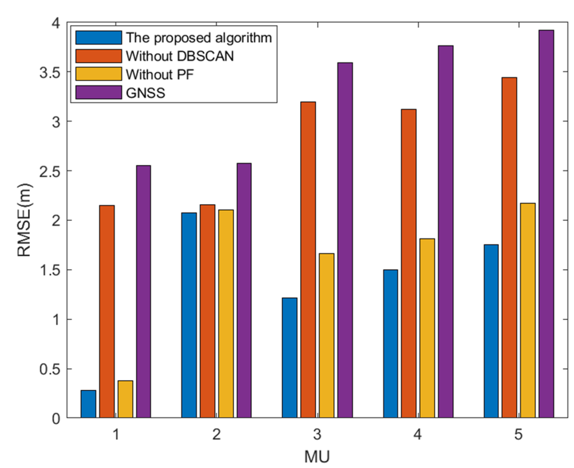
To evaluate the effect of DBSCAN and PF in our proposed algorithm, we compare GITPA with the following three situations:

• Without DBSCAN: As we know, the position information of the cooperative nodes is inaccurate. Specifically, here we use the inaccurate position information of the cooperative nodes with the GNSS and TOA/RSS measurements to calculate the positions of the requesting nodes by GITPAPF. In other words, we want to see how the inaccurate position information of the cooperative nodes influence the position results of the requesting nodes.
• Without PF: Here, we only keep the clustering process based on DATM with the joint TOA/RSS method and output the mean value of the clusters as the final results for the positions of the requesting nodes. That is, we omit the PF process in this algorithm, and the performance of PF in the proposed algorithm can be demonstrated.
• GNSS: The GNSS measurements are directly calculated to obtain the positions of the requesting nodes without any integration with the measurements from the 5G network.

From Figure 5, it is clear that the proposed algorithm, which synthesizes the DBSCAN and PF, achieves the best performance towards the root-mean-square errors (RMSEs) compared to other algorithms. Compared to the GNSS positioning, the lowest improvement of the proposed algorithm in RMSE is nearly 20%, appearing in MU 2, and the highest is approximately 85%, appearing in MU 1. Besides the GNSS results, which contain no additional processing and act as one kind of measurement source in our proposed algorithm, the algorithm without DBSCAN performs the worst, and the algorithm without PF achieves better than that. It explains that the inaccurate position information of the cooperative nodes can cause large errors in the positions of the requesting nodes. Thus, if the known positions of the reference nodes for the requesting nodes are inaccurate, it is hard to obtain accurate positions of the requesting nodes. In this regard, the improvement of the PF in that case is limited.

To analyze the effect of the TOA and RSS measurements in our proposed algorithm, we compare GITPA with three other situations:

• With TOA only: We only use TOA measurements to estimate the distances between the requesting nodes and the reference nodes, including the BSs and the cooperative nodes, which are further exploited in DBSCAN and PF processes in our proposed algorithm.
• With RSS only: Similarly, the RSS measurements are solely exploited in the proposed algorithm.
• GNSS: As mentioned above, the GNSS positioning results are directly added for comparison to illustrate the effect of TOA and RSS measurements more comprehensively.

Figure 6 illustrates the performance comparison between the proposed algorithm and the above three algorithms for the five requesting nodes. It is obvious that the proposed algorithm that utilizes both TOA and RSS measurements obtains the lowest RMSEs for all the requesting nodes, and the GNSS positioning obtains the highest. From Figure 6, we can see that there is no clear difference between the algorithms based on the TOA and RSS measurements separately, and these two algorithms achieve a little worse than the proposed algorithm. This is because the distance between a requesting node and its reference nodes may be long or short, and the TOA and RSS measurements affect the range estimation in an average way. Note that when there is limited measurement information or computational resources, it is also feasible to use only TOA or RSS measurements.

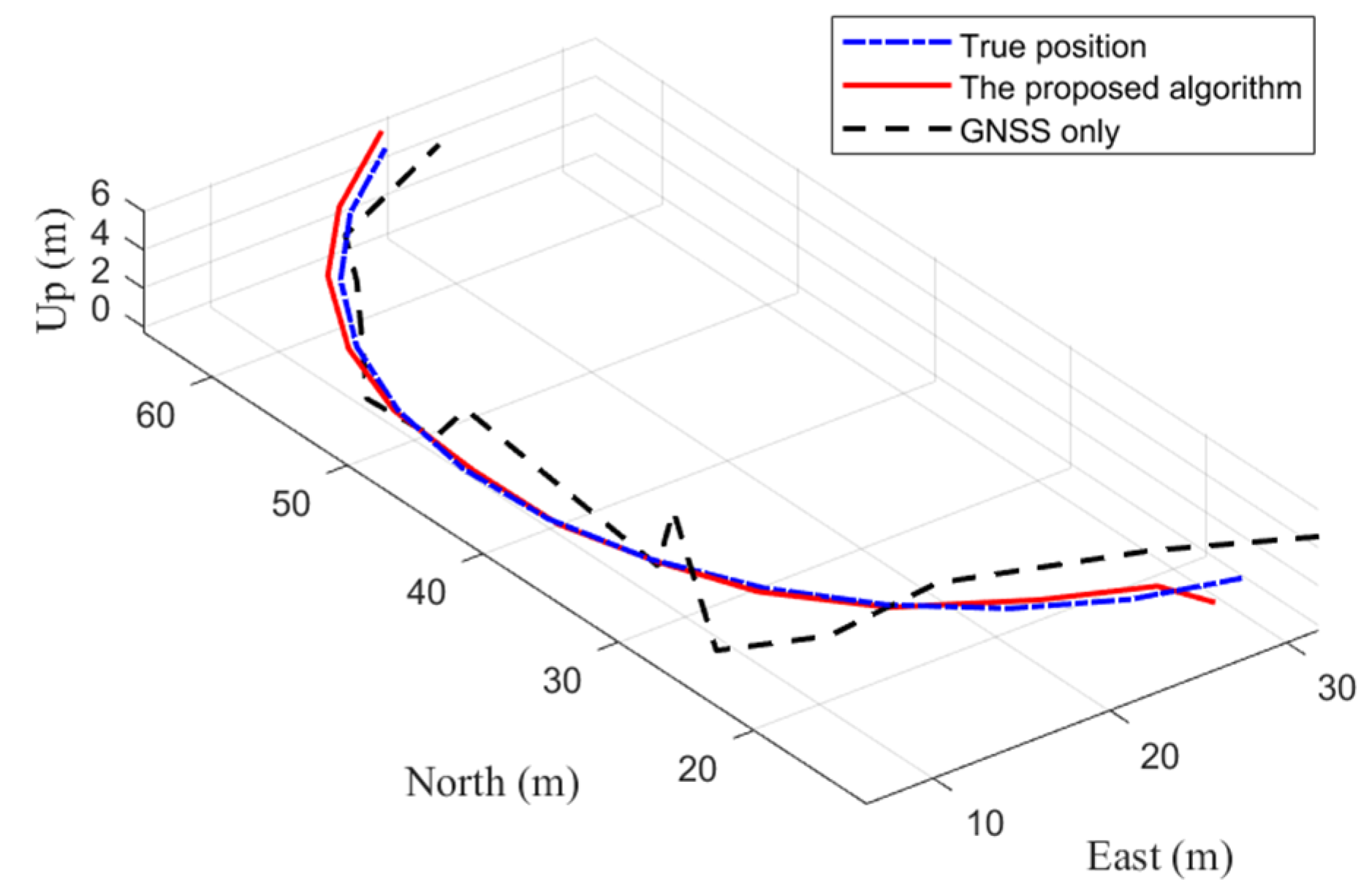
To analyze the performance of the proposed algorithm when the requesting node is moving, we plot Figure 7 to see the positioning results where the requesting node moves at a fixed linear velocity and angular velocity. As is shown in Figure 7, the blue chain dotted line represents the trajectory of the requesting node, the red solid line represents the positions calculated by our proposed algorithm and the black dashed line represents the positions from the GNSS measurements. It is clear that the red solid line nearly coincides with the blue chain dotted line, meaning that the error in the results of the proposed algorithm for a moving requesting node is small, and it proves that the proposed algorithm is also effective for the moving requesting nodes.

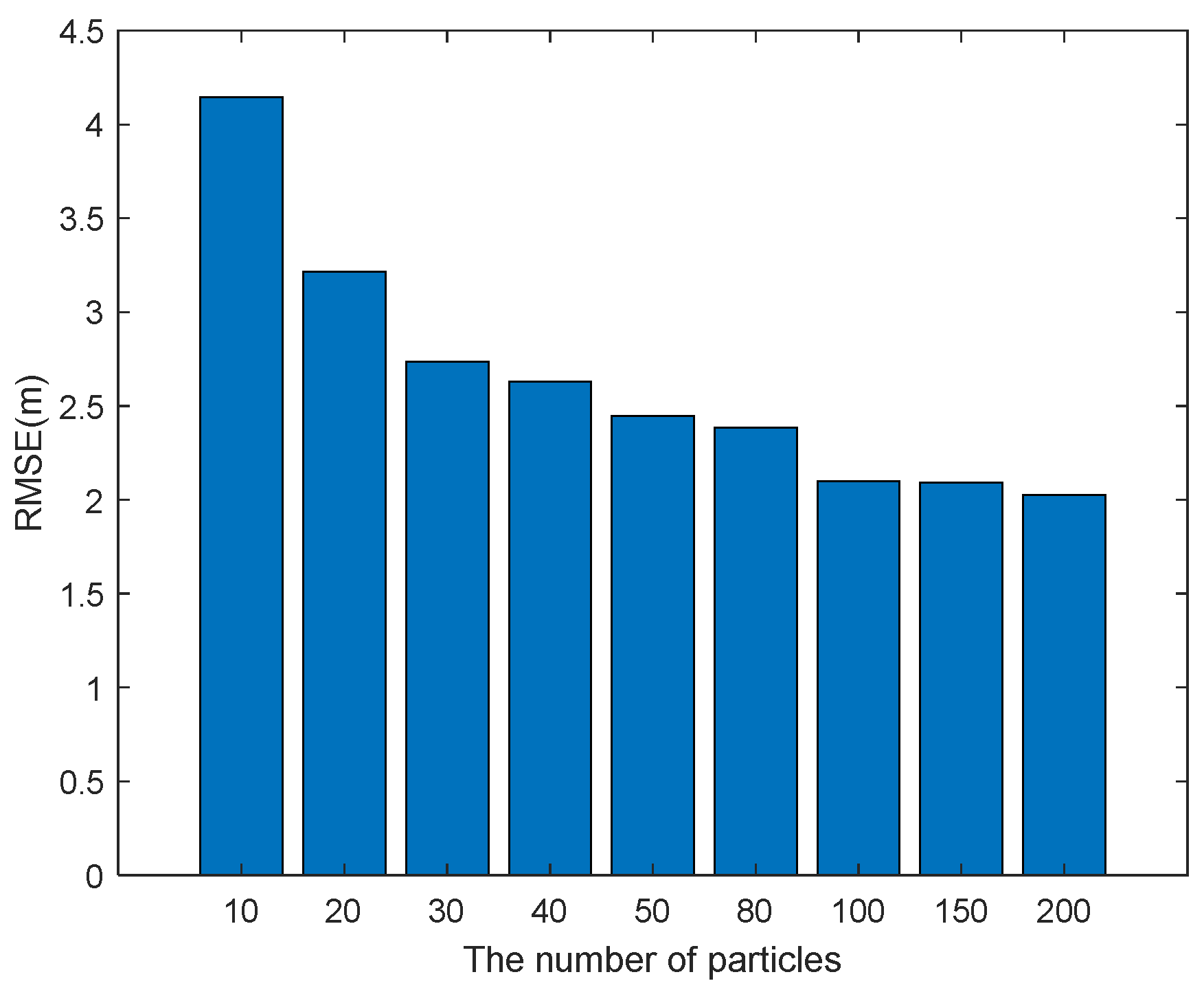
Figure 8 shows the RMSEs with different numbers of the particles used in the PF process. We can see that the RMSE decreases as the number of the particles increases. As we know, more particles can result in better performance of the PF. It is also obvious that the improvement is slight as we increase the number of the particles under circumstance of conducting the DBSCAN process in advance. Moreover, it is clear that the improvement of RMSE is really small when the number of the particles exceeds 100. Thus, to guarantee the performance, as well as to save the computational resources, we choose 100 particles in our numerical simulation.

4. Discussion

The proliferation of various LBSs requires more precise and reliable positioning, whereas the emergence of 5G provides new visions for positioning. Its disruptive technologies are expected to achieve high-accuracy positioning, such as D2D communication, ultra-dense network, edge computing and mmWave communication. Thus, the combination of GNSS and 5G to provide accurate positioning has attracted much attention from researchers. Especially, D2D communication allows two MUs in proximity to communicate directly without being relayed by the BS, which makes it possible for a requesting user to connect other MUs and obtain more measurements for positioning. Actually, unlike the BSs, many MUs know their positions while the information is not accurate. We exploited the DBSCAN algorithm to reduce the uncertainty of their position information, and the positions of the requesting nodes were also obtained based on the GNSS and TOA/RSS measurements in the 5G network. After that, the PF algorithm was utilized to further improve the positioning accuracy of the requesting nodes.

There are some conclusions based on the numerical simulation results as follows:

• It is clear in Figure 4 that, after the clustering, the data points that represent the positions of the MUs with high density gather in clusters, while the abnormal data points are deleted. In this case, the cooperative nodes can obtain more accurate position information, as well as the requesting nodes.
• We can see in Figure 5 that, in the circumstance of inaccurate cooperative nodes’ positions, we can hardly achieve accurate positioning for the requesting nodes with the PF algorithm only. Nevertheless, the positioning accuracy can be further improved by the PF algorithm after the DBSCAN process.
• The joint TOA/RSS method was used in our scheme since these two kinds of measurements can complement each other with different advantages. Figure 6 verifies that the joint TOA/RSS method can achieve the best performance compared with the algorithms with only one kind of measurement.
• Figure 7 illustrates the positioning performance of the proposed algorithm when the requesting node is on the move, and it proves that the algorithm also suits the dynamic condition well.
• In terms of PF, it is found in Figure 8 that more particles result in lower RMSEs for positioning, which is consistent with the property of the PF algorithm.

Certainly, there are still some problems in need of investigation. Although we exploited edge computing to relieve the computation burden of the MUs and the network, there are still some key aspects to be solved, such as the computation task model and task scheduling, and how to integrate edge computing and positioning in a physical level is of great importance. Moreover, as discussed above, mmWave communication in 5G enables high separation of the multipath component with very large signal bandwidth, and then, only the dominant path exists in the channel estimation process. Besides, it adopts directional beamforming, with which the angle-related measurements can be accurately extracted. Hence, it is promising to provide high accuracy positioning if it is combined with D2D communication. For further study, we wish to focus on a deep combination of the GNSS/5G integrated positioning with the edge computing, as well as mmWave communication to achieve better positioning performance.

5. Conclusions

In this paper, we studied the GNSS/5G integrated three-dimensional positioning based on D2D communication. The TOA and RSS measurements were combined based on the signal propagation models in the 5G network to estimate the distances between the requesting nodes and the reference nodes, including the BSs and the cooperative nodes. To tackle the problem of inaccurate position information of the cooperative nodes, we proposed a DBSCAN algorithm based on the GNSS measurements and the joint TOA/RSS method. Hence, we obtained integrated positions of the requesting nodes and more accurate positions of the cooperative nodes. Then, a PF algorithm based on TOA/RSS measurements was proposed to further integrate the above results. Simulation results demonstrated that our proposed algorithm brings substantial performance improvement towards the RMSEs of the requesting nodes, whether they are fixed or on the move. Moreover, the proposed algorithm not only performed better than the other algorithms when the DBSCAN or PF algorithm is separately exploited, but it was also better than the algorithms using only the TOA or RSS measurements.

References

- Taranto, R.D.; Muppirisetty, S.; Raulefs, R.; Slock, D.; Svensson, T.; Wymeersch, H. Location-aware communications for 5G networks: How location information can improve scalability, latency, and robustness of 5G. IEEE Signal Process. Mag. 2014, 31, 102–112. [Google Scholar] [CrossRef] [Green Version]
- Zekavat, R.; Buehrer, R.M. Handbook of Position Location: Theory, Practice and Advances, 2nd ed.; John Wiley & Sons: New York, NY, USA, 2018. [Google Scholar] [CrossRef]
- Ioannides, R.T.; Pany, T.; Gibbons, G. Known vulnerabilities of global navigation satellite systems, status, and potential mitigation techniques. Proc. IEEE 2016, 104, 1174–1194. [Google Scholar] [CrossRef]
- Yang, Y.; Mao, Y.; Sun, B. Basic performance and future developments of BeiDou global navigation satellite system. Satell. Navig. 2020, 1, 1. [Google Scholar] [CrossRef] [Green Version]
- Yang, Y.; Liu, L.; Li, J.; Yang, Y.; Zhang, T.; Mao, Y.; Sun, B.; Ren, X. Featured services and performance of BDS-3. Sci. Bull. 2021, 66, 2135–2143. [Google Scholar] [CrossRef]
- Yang, Y.; Ding, Q.; Gao, W.; Li, J.; Xu, Y.; Sun, B. Principle and performance of BDSBAS and PPP-B2b of BDS-3. Satell. Navig. 2022, 3, 5. [Google Scholar] [CrossRef]
- Yang, Y. Concepts of comprehensive PNT and related key technologies. Acta Geod. Cartogr. Sin. 2016, 45, 505–510. [Google Scholar] [CrossRef]
- Yang, Y. Resilient PNT concept frame. J. Geod. Geoinf. Sci. 2019, 2, 1–7. [Google Scholar] [CrossRef]
- Yin, L.; Ni, Q.; Deng, Z. Intelligent multisensor cooperative localization under cooperative redundancy validation. IEEE Trans. Cybern. 2021, 51, 2188–2200. [Google Scholar] [CrossRef] [Green Version]
- Peral-Rosado, J.A.; Saloranta, J.; Destino, G.; López-Salcedo, J.A.; Seco-Granados, G. Methodology for simulating 5G and GNSS high-accuracy positioning. Sensors 2018, 18, 3220. [Google Scholar] [CrossRef] [Green Version]
- Peral-Rosado, J.A.; Raulefs, R.; López-Salcedo, J.A.; Seco-Granados, G. Survey of cellular mobile radio localization methods: From 1G to 5G. IEEE Commun. Surv. Tutor. 2018, 20, 1124–1148. [Google Scholar] [CrossRef]
- Wymeersch, H.; Seco-Granados, G.; Destino, G.; Dardari, D.; Tufvesson, F. 5G mmWave positioning for vehicular networks. IEEE Wirel. Commun. 2017, 24, 80–86. [Google Scholar] [CrossRef] [Green Version]
- Angelis, G.; Baruffa, G.; Cacopardi, S. GNSS/Cellular hybrid positioning system for mobile users in urban scenarios. IEEE Trans. Intell. Transp. Syst. 2013, 14, 313–321. [Google Scholar] [CrossRef]
- Hein, G.W. Status, perspectives and trends of satellite navigation. Satell. Navig. 2020, 1, 22. [Google Scholar] [CrossRef] [PubMed]
- Liu, J.; Gao, K.; Guo, W.; Cui, J.; Guo, C. Role, path, and vision of “5G + BDS/GNSS”. Satell. Navig. 2020, 1, 23. [Google Scholar] [CrossRef]
- Destino, G.; Saloranta, J.; Seco-Granados, G.; Wymeersch, H. Performance analysis of hybrid 5G-GNSS localization. In Proceedings of the 2018 52nd Asilomar Conference on Signals, Systems, and Computers, Pacific Grove, CA, USA, 28–31 October 2018. [Google Scholar] [CrossRef] [Green Version]
- Jo, M.; Maksymyuk, T.; Strykhalyuk, B.; Cho, C. Device-to-device-based heterogeneous radio access network architecture for mobile cloud computing. IEEE Wirel. Commun. 2015, 22, 50–58. [Google Scholar] [CrossRef]
- Wei, L.; Hu, R.Q.; Qian, Y.; Wu, G. Enable device-to-device communications underlaying cellular networks: Challenges and research aspects. IEEE Commun. Mag. 2014, 52, 90–96. [Google Scholar] [CrossRef]
- Dammann, A.; Raulefs, R.; Zhang, S. On prospects of positioning in 5G. In Proceedings of the 2015 IEEE International Conference on Communication Workshop (ICCW), London, UK, 8–12 June 2015. [Google Scholar] [CrossRef]
- Wymeersch, B.H.; Lien, J.; Win, M.Z. Cooperative localization in wireless networks. Proc. IEEE 2009, 97, 427–450. [Google Scholar] [CrossRef]
- Dai, W.; Shen, Y.; Win, M.Z. Energy-efficient network navigation algorithms. IEEE J. Sel. Areas Commun. 2015, 33, 1418–1430. [Google Scholar] [CrossRef]
- Coluccia, A.; Ricciato, F.; Ricci, G. Positioning based on signals of opportunity. IEEE Commun. Lett. 2014, 18, 356–359. [Google Scholar] [CrossRef]
- Coluccia, A.; Fascista, A. On the hybrid TOA/RSS range estimation in wireless sensor networks. IEEE Trans. Wirel. Commun. 2018, 17, 361–371. [Google Scholar] [CrossRef]
- Catovic, A.; Sahinoglu, Z. The Cramer-Rao bounds of hybrid TOA/RSS and TDOA/RSS location estimation schemes. IEEE Commun. Lett. 2004, 8, 626–628. [Google Scholar] [CrossRef]
- Prieto, J.; Mazuelas, S.; Bahillo, A.; Fernández, P.; Lorenzo, R.M.; Abril, E.J. Adaptive data fusion for wireless localization in harsh environments. IEEE Trans. Signal Process. 2012, 60, 1585–1596. [Google Scholar] [CrossRef]
- Thrun, S.; Burgard, W.; Fox, D. Probabilistic Robotics; MIT Press: Cambridge, MA, USA, 2005. [Google Scholar]
- Mensing, C.; Sand, S.; Dammann, A. Hybrid data fusion and tracking for positioning with GNSS and 3GPP-LTE. Int. J. Navig. Obs. 2010, 2010, 812945. [Google Scholar] [CrossRef]
- Yin, L.; Ni, Q.; Deng, Z. A GNSS/5G integrated positioning methodology in D2D communication networks. IEEE J. Sel. Areas Commun. 2018, 36, 351–362. [Google Scholar] [CrossRef]
- Zhang, J.; Yang, F.; Deng, Z.; Fu, X.; Han, J. Research on D2D co-localization algorithm based on clustering filtering. China Commun. 2020, 17, 121–132. [Google Scholar] [CrossRef]
- Mao, Y.; You, C.; Zhang, J.; Huang, K.; Letaief, K.B. A survey on mobile edge computing: The communication perspective. IEEE Commun. Surv. Tutor. 2017, 19, 2322–2358. [Google Scholar] [CrossRef] [Green Version]
- 3GPP. Study on Channel Model for Frequencies from 0.5 to 100 GHz; 3rd Generation Partnership Project (3GPP), TR 38.901 V14.0.0. 2017. Available online: https://www.3gpp.org/ftp//Specs/archive/38_series/38.901/38901-e00.zip (accessed on 7 March 2022).
- Kantardzic, M. Data Mining: Concepts, Models, Methods, and Algorithms, 3rd ed.; John Wiley & Sons: New York, NY, USA, 2011. [Google Scholar] [CrossRef]
- Zhou, Z. Machine Learning; Tsinghua University Press: Beijing, China, 2016. [Google Scholar]
- Schubert, E.; Sander, J.; Ester, M.; Kriegel, H.; Xu, X. DBSCAN revisited, revisited: Why and how you should (still) use DBSCAN. ACM Trans. Database Syst. 2017, 42, 1–21. [Google Scholar] [CrossRef]
- Sui, L.; Song, L.; Chai, H.; Liu, C. Error Theory and Foundation of Surveying Adjustment, 2nd ed.; Survey and Mapping Press: Beijing, China, 2018. [Google Scholar]
- Simon, D. Optimal State Estimation: Kalman, H∞, and Nonlinear Approaches; John Wiley & Sons: New York, NY, USA, 2006. [Google Scholar] [CrossRef]
- Siciliano, B.; Khatib, O. Springer Handbook of Robotics; Springer: New York, NY, USA, 2008. [Google Scholar] [CrossRef]
- Luo, J.; Wang, Z. Multi-Source Data Fusion and Sensor Management; Tsinghua University Press: Beijing, China, 2015. [Google Scholar]
- Zhao, S.; Zhang, X.-P.; Cui, X.; Lu, M. Optimal two-way TOA localization and synchronization for moving user devices with clock drift. IEEE Trans. Veh. Technol. 2021, 70, 7778–7789. [Google Scholar] [CrossRef]
Figure 1.
System model of GNSS/5G three-dimensional integrated positioning.
Figure 2.
Two-dimensional positioning based on trilateration: (a) the positioning procedure when the positions of three reference nodes are accurate, and (b) the comparison between the positioning procedure with accurate and inaccurate reference nodes.
Figure 3.
The basic definitions of DBSCAN.
Figure 4.
Distribution of the data points before (a) and after (b) the DBSCAN process based on the TOA measurements.
Figure 5.
Performance comparison between the proposed algorithm and other situations for the requesting nodes.
Figure 6.
Performance comparison between the algorithms based on different measurements for the requesting nodes.
Figure 7.
Positioning results of a moving MU.
Figure 8.
RMSEs versus the number of particles.