
Spatial Potential Energy Weighted Maximum Simplex Algorithm for Hyperspectral Endmember Extraction

1
Information Science and Technology College, Dalian Maritime University, Dalian 116026, China
2
Zhengzhou Tobacco Research Institute of CNTC, Zhengzhou 450001, China
*
Author to whom correspondence should be addressed.
Remote Sens. 2022, 14(5), 1192; https://doi.org/10.3390/rs14051192
Submission received: 18 January 2022
/
Revised: 19 February 2022
/
Accepted: 23 February 2022
/
Published: 28 February 2022
(This article belongs to the Special Issue Recent Advances in Processing Mixed Pixels for Hyperspectral Image)
Abstract
:Most traditional endmember extraction algorithms focus on spectral information, which limits the effectiveness of endmembers. This paper develops a spatial potential energy weighted maximum simplex algorithm (SPEW) for hyperspectral endmember extraction, combining the relevance of hyperspectral spatial context with spectral information to effectively extract endmembers. Specifically, for pixels in a uniform spatial area, SPEW assigns a high weight to pixels with higher spatial potential energy. For pixels scattered in a spatial area, the high weights are assigned to the representative pixels with a smaller spectral angle distance. Then, the optimal endmember collection is determined by the simplex with maximum volume in the space of representative pixels. SPEW not only reduces the complexity of searching for the maximum simplex volume but also improves the performance of endmember extraction. In particular, compared with other newly proposed spatial-spectral hyperspectral endmember extraction methods, SPEW can effectively extract the hidden endmembers in a spatial area without adjusting any parameters. Experiments on synthetic and real data show that the SPEW algorithm has also provides better results than the traditional algorithms.
1. Introduction
Hyperspectral remote sensing image data has the characteristics of a wide range of spectral bands and high spectral resolution. However, the existence of mixed pixels reduces the accuracy of traditional pixel-level data operation, so the decomposition of mixed pixels is an important task in processing of hyperspectral images. In hyperspectral images (HSIs), the pure pixels that contain only one kind of terrain information are called endmembers, and the fractions of each endmember in the pixels are called abundances [1,2,3].
Typical endmember extraction algorithms based on convex geometry are widely used in linear spectral unmixing. Among them, pure pixel index (PPI) [4] involves projecting all pixels onto a set of randomly generated unit vector. Commonly, the mixed pixels will be projected to the middle, and the endmembers will be projected to the endpoints of vector. The times of each pixel being projected to the endpoints is recorded as pure pixel index, and the pixel with the highest PPI is selected as the endmember. Automatic target generation process (ATGP) [5] also utilizes orthogonal projection to find the largest residual vector as the endmember. The vertex component analysis (VCA) [6] algorithm can be viewed as a variant of PPI based on convex cones, which uses the geometric fact that the seven endmembers are usually the vertex of a simplex. The N-FINDR [7,8] algorithm finds the maximum simplex from the convex simplex in the hyperspectral feature space to obtain all endmembers simultaneously. As a variant of N-FINDR, the simplex growth algorithm (SGA) [9] aims to find a series of maximum simplexes with different numbers of vertices and extract the vertices of the simplexes as endmembers one by one.
At the same time, the non-negative matrix factorization algorithm (NMF) [10] has attracted considerable attention because of its ability to extract endmembers and estimate abundance at the same time. The NMF algorithm decomposes the data matrix into two non-negative submatrices, which is equivalent to the product of the endmember matrix and the abundance matrix. However, the NMF algorithm tends to fall into local extreme values and cannot guarantee a unique solution. Geometric constraints are added to the algorithm later, such as the minimum volume constrained NMF algorithm (MVC-NMF) [11], sparsity CNMF ( NMF) [12], etc.
Extracting endmembers by spectrum property ignores the spatial distribution or structural information, resulting in a limited unmixing performance. Therefore, some algorithms combining spectral features with spatial features have emerged [13,14,15,16,17,18,19,20,21,22,23]. The earliest unmixing algorithm using spatial-spectral features is automated morphological endmember extraction (AMEE) [24], which extends mathematical morphology into multidimensional domains and defines a set of spatial-spectral operations to automatically extract endmembers. In addition, the spatial purity-based endmember extraction algorithm (SPEE) [25], region-based spatial preprocessing (RBSPP) [26] and spatial-spectral preprocessing (SSPP) [27] have emerged. The SPEE method estimates a scalar spatial weighting factor for each pixel vector, which is related to the spectral similarity of pixels located in a spatial neighborhood. RBSPP is a spatial preprocessing module, which combines unsupervised clustering with orthogonally subspace projection to automatically search the region with uniform spectrum and extract endmembers in these regions. As a spatial spectrum preprocessing module, SSPP first deduces the spatial homogeneity index of each pixel, At the same time, SSPP performs unsupervised clustering. Finally, it selects a subset of spatially uniform pixel and spectral pure pixel from each cluster to fuse spatial information and spectral information together to form candidate endmembers.
Many research works on spatial-spectral unmixing have been carried out recently. The authors of [28] proposed that spatial processing could be used for pre-processing or post-processing of the spectrum. The data matrix was reconstructed according to the linear relationship between pixels and their neighborhoods. To reduce local spectral changes, sparse representation was added, and the singular value decomposition method was used to reconstruct the adjacent pixels of the main feature. Entropy-based convex set optimization for spatial-spectral endmember extraction (ECSO) [29] was proposed by Shah et al. For the first time, the spatial information of entropy was used in hyperspectral unmixing, combined with convex set optimization to extract endmembers. According to the entropy, the algorithm can characterize the spatial heterogeneity of each band. The feature of the low-entropy bands containing homogeneous objects, and the high-entropy bands containing heterogeneous objects, improved the accuracy of extracting rare and abnormal endmembers. The spatial energy prior constrained maximum simplex volume approach (SENMAV) [30] was proposed by Shen et al., which utilized the spatial energy prior constraint method to impose spatial constraints on the maximum simplex. This spatial constraint principle comes from the Markov Random Field (MRF) [31,32,33,34,35], with the assumption that adjacent pixels are more likely to belong to the same category, and the spatial energy is calculated. The larger the spatial energy, the more advantageous the structure of the maximum simplex. To adjust the proportion of spectral features and spatial features, it is necessary to set the balance parameter between maximum simplex and spatial energy. However, it is difficult to determine the parameter for different datasets, which brings great instability to the result of unmixing. On the other hand, SENMAV is sensitive to large-class endmembers, and cannot effectively identify small-class endmembers, especially those with a divergent spatial distribution.
Therefore, this paper proposes a maximum simplex algorithm based on spatial potential energy (SPEW) to extract endmembers, which weights each pixel by the space potential energy of MRF. In this way, the spatial and spectral features can be fused, and the uncertainty of equilibrium parameters in different datasets can be solved. In order to overcome the problem of ignoring endmembers in the scattered region of pixel categories, we introduce spectral angular distance to search for spectral representative pixels with low spatial potential energy and treat them as candidate endmembers to construct the maximum simplex. Therefore, SPEW is not only accurate for finding representative pixels in uniform regions of hyperspectral data images but also effective in the recognition of distributed endmembers in heterogeneous regions.
2. Relative Research Works
2.1. LMM
The hyperspectral mixing models essentially contain linear and nonlinear models. The linear mixture model (LMM) assumes that there is no interaction between objects, and each photon only interacts with one substance. When multiple scattering occurs between substances, the nonlinear mixture model is developed according to the actual situation. LMM is most broadly used in hyperspectral unmixing for its algorithmic simplicity, physical significance and practical efficiency [36].
According to the linear mixed model, the hyperspectral image Y with pixels is expressed in the following form:
where is any spectral vector with bands in the image Y. is the number of endmembers, and is the endmember matrix of . is the abundance vector of pixel y. is the noise of pixel y.
The abundance map is required to satisfy two physical constraints, the abundance sum-to-one constraint (ASC):
and the abundance non-negative constraint (ANC):
2.2. Space Energy
The space energy principle comes from the planar grid structure of the two-dimensional MRF, where each variable clearly depends on neighboring groups rather than itself and can be compared. The neighborhood system is used to analyze the Markov property in space. Therefore, the relationship between the eight neighborhood pixels closest to the current pixel is mainly concerned in space, and the space potential energy is constructed according to the degree of similarity.
Let be a set of general neighborhood systems defined on . There are different neighborhood structures in . On , a single-pixel or a subset of pixels and its neighbors is , the set of sub-clusters is denoted by .
Using the probability distribution in Gibbs, if and only if the joint probability distribution of the random field is as follows:
Among them, is the energy function. is the clique potential function, and it is only related to the sub-cluster where the pixel is located. , as a normalization constant, is the partition function.
The definition of the clique potential function is related to the assigned label value, which is defined as:
where is a neighborhood pixel with as the center belonging to the cluster , and is a coupling coefficient to indicate the correlation between the center pixel and the pixels in the neighborhood.
2.3. SENMAV
The SENMAV algorithm first converts the hyperspectral image Y to by PCA as dimensionality reduction method. Then, K-means [37] clustering is used to generate the classification label . According to the classification labels of the center pixel and its neighborhood pixels, the spatial energy is calculated as follows:
represents the ith pixel selected from .
The simplex volume is defined as:
The endmember collection is determined iteratively by the objective of highest energy in space and the maximum simplex volume.
where . As a balance parameter between space energy and spectral information, needs to be adjusted on different datasets, which has a great impact on the unmixing effect.
3. Spatial Potential Energy Weighted Maximum Simplex Algorithm
3.1. Space Potential Energy Weighting
Here, in our model, the spatial energy is assigned for each pixel. The spatial potential energy is the total energy of the pixel clusters and its neighbors. The more similarity between the central pixel and its neighboring pixels, the greater the potential energy, which is determined by judging whether the center pixel classification label is the same as the neighborhood label. Here, the K-means unsupervised clustering algorithm is used to generate classes, and each pixel is assigned a class label mapping. The number of classes is a reasonable estimate considering the calculation complexity of K-means and the number of endmembers [30].
Before using K-means clustering, it is also necessary to perform PCA dimensionality reduction on the spectral image to bands, so that . In addition, PCA may achieve good denoising effect. The process of determining the classification labels and cluster centers by K-means is defined as follows:
Among them, represents the mapping from pixels to category labels, and is the centroid pixels with bands. Let be a neighborhood centered on the ith pixel, the spatial potential energy of the pixels can be defined as:
where represents the potential energy of the ith pixel, and represents the classification label of the ith pixel, where
is the clique potential function of the ith pixel in the neighborhood .
Based on the assumption that the greater the similarity between a pixel and its neighboring pixels, the more likely the pixel and its neighbors belong to the same category, it can be inferred that the greater the spatial potential of a pixel, the greater the possibility that it is an effective endmember. Pick the pixels with high potential energy:
where is the set of l pixels with high potential energy, and is the index of . When the potential energy is maximum, the center pixel is the same as all the pixel class labels in the neighborhood.
Next, assign a spatial weight to the ith pixel, as shown in the following expression:
By setting the spatial potential energy weight to 1, the algorithm can simply and effectively eliminate the area with a high spatial mixing degree, and it can minimize the interference of spatial mixing pixels on the endmember selection of uniformly distributed areas. It is efficient for the endmember selection of large categories. However, at the same time, the problem arises that the scattered endmembers of the small category will be ignored consequently. Furthermore, as described in the following section, we involved the spectral distance to include the missing category pixels.
3.2. Spectral Distance Weighting
The spatial potential energy of a pixel has a very large correlation with the pixel neighborhood. It provides great convenience for finding the endmembers in the uniform region. However, there is a case that the distribution of a certain substance is divergent, and the pixels are less similar to those in the surrounding neighborhood. Therefore, the minimum spectral angle distance is introduced to make up for the defects caused by the space potential energy weighting method. It is believed that the smaller the spectral distance between two pixels, the more similar the two pixels. In the pixel categories where there is no candidate endmember selected out by spatial potential energy, some pixels with small spectral angle distance from all other pixels are selected as candidate endmembers.
First, the pixel category is not selected by spatial potential energy, and the spectral angle distance between a pixel and all other pixels of the category is calculated.
The number of pixels less than the spectral angle distance threshold is counted. If the number is large enough, a valid weight is given to the pixel as a candidate endmember.
A proper threshold value can make the pixels selected by the spectral angle distance method more representative. Suppose the level of the spectral angle distance value is . The OTSU algorithm can regard the distances as two classes according to the level , namely and , and calculate the variance of between classes:
, is the probability that the spectral angle distance value belongs to the ith level in this class, . The spectral angle distance is the accumulated mean value of level , the global mean value , and the threshold is obtained according to the corresponding level when the inter-class variance is the largest.
In the same way, the threshold of the number of similar pixels to the current pixel can be obtained.
3.3. SPEW Algorithm
Based on the pure pixel hypothesis, the simplex volume composed of p endmembers is the largest.
Iteratively update the pixels that compose the simplex to obtain the maximum simplex volume.
SPEW is to strengthen the pixels with high potential energy and weaken the pixels with low potential energy. Finally, the weighted pixels that compose the maximum simplex are regarded as endmembers. The objective function is as follows:
Combining the hyperspectral spatial information and spectral information as the weight to identify endmembers, this algorithm effectively avoids calculation of the scaling factor and adjusting factor for regulation in SEMAV, and extracts discrete endmembers might of great significance.
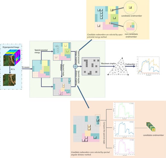
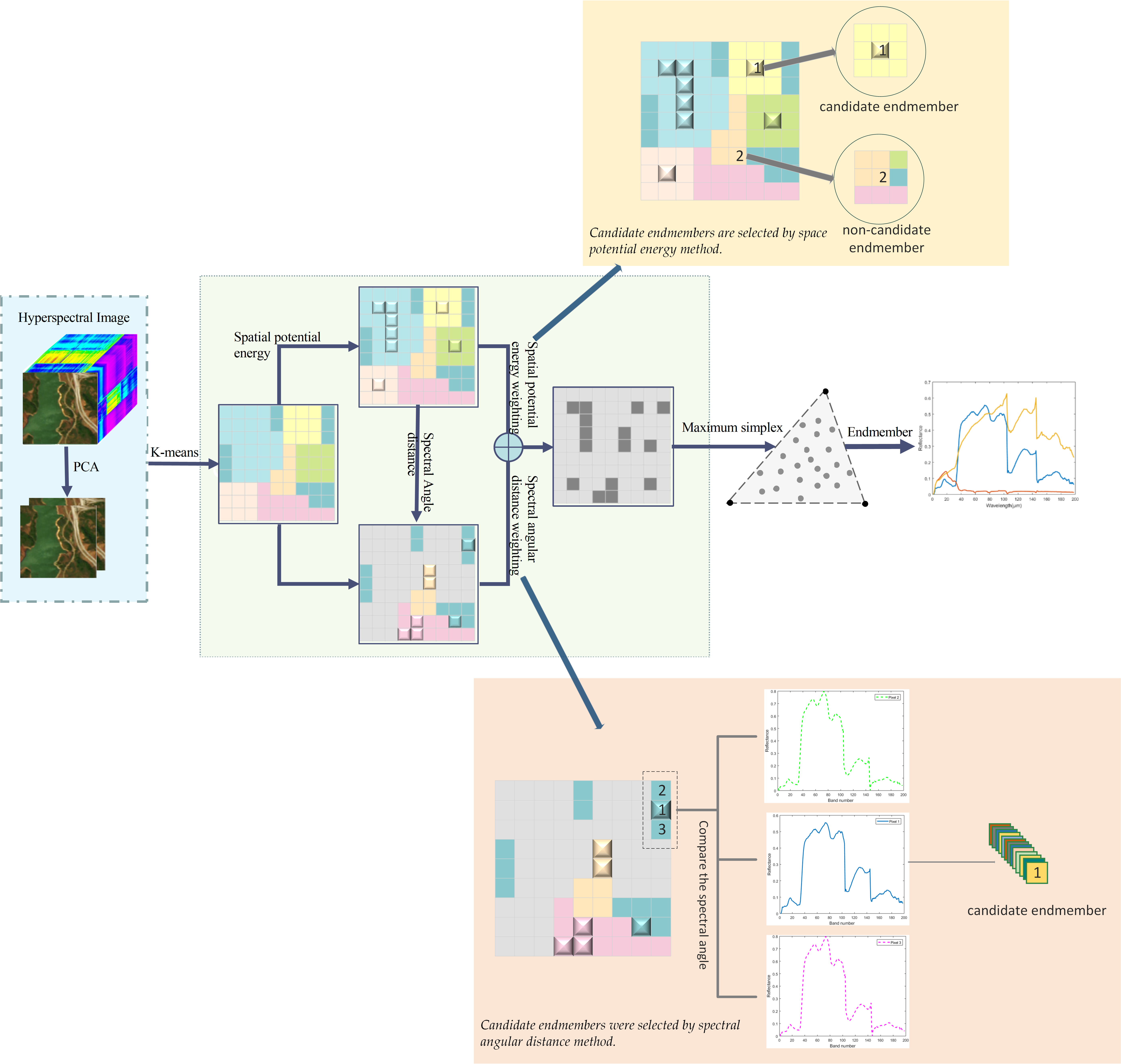
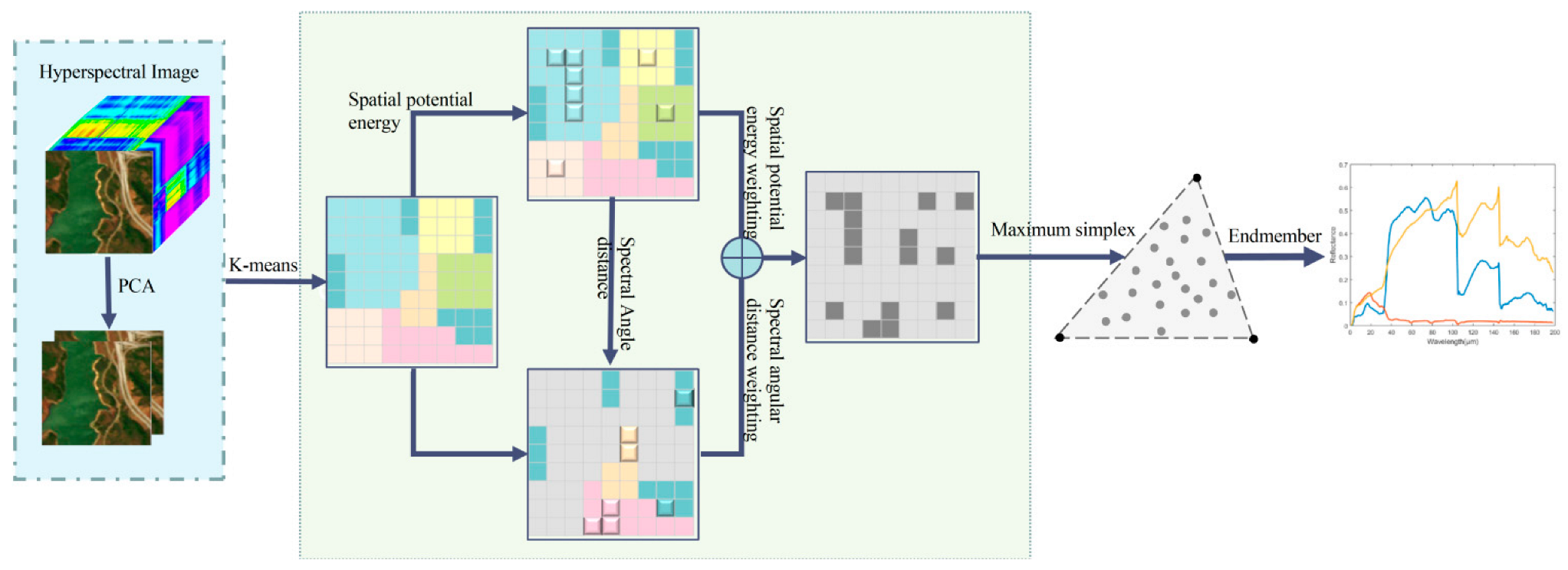
Figure 1 describes the framework of SPEW. First, PCA dimensionality reduction was performed on the input hyperspectral image, and K-means unsupervised clustering method was used to assign classification labels to all pixels. After that, the spatial potential energy of each pixel was calculated, where the more neighboring pixels of the same pixel category, the greater the spatial potential energy. Pixels with larger spatial potential energy were weighted by 1, and the rest by 0. This operation was performed on the pixels of the whole image, and some scattered small-class pixels were ignored against the large-weight categories. Therefore, the spectral angle distance value was calculated for the pixels in such category. If the spectral angle distance is small, it means that the pixels are similar. The larger the number of similar pixels, the more representative they are, so the weight of such pixels was also set to 1. These two operations can greatly reduce the number of candidate pixels, thereby effectively reducing the interference of similar endmembers. Finally, the final endmembers were determined by the maximum simplex volume.
4. Experimental Results and Analysis
The algorithm SPEW was compared with several endmember extraction algorithms based on the pure pixel hypothesis on real datasets and synthetic datasets, including VCA, ATGP, SGA, SENMAV and ECSO.
4.1. Evaluation Criteria
Spectral angular distance (SAD) was used to determine the similarity between spectra by calculating the angle between them. The smaller the value of SAD, the more similar the two spectra.
where represents the ith real endmember vector, and represents the obtained endmember vector corresponding to this real endmember. The root mean square error (RMSE) was used to calculate the error between the obtained abundance vector and the true abundance vector. The smaller the RMSE value, the more accurate the abundance estimation.
where represents the abundance vector corresponding to ith pixel, and represents the estimated abundance vector corresponding to .
The reconstruction error (RE) was used to reconstruct the data matrix using the extracted endmembers and abundance maps , and to compare it with the original data. If the reconstructed matrix is more similar to the original data , then the RE value is smaller.
These measurement indicators evaluate the algorithms from different aspects. SAD is the criterion for the extracted endmembers, which directly compute the similarity between the evaluated endmembers and real endmembers. The RMSE criterion is an indirect verification for a pure endmember extraction algorithm because the calculating the abundance also relies on the abundance estimating method. The RE calculates the error between the original image and the reconstruction image wholly. These indicators are helpful to verify the unmixing performance of the test algorithms completely, including endmember extraction and abundance estimation.
4.2. Experimental Dataset
4.2.1. Synthetic Dataset
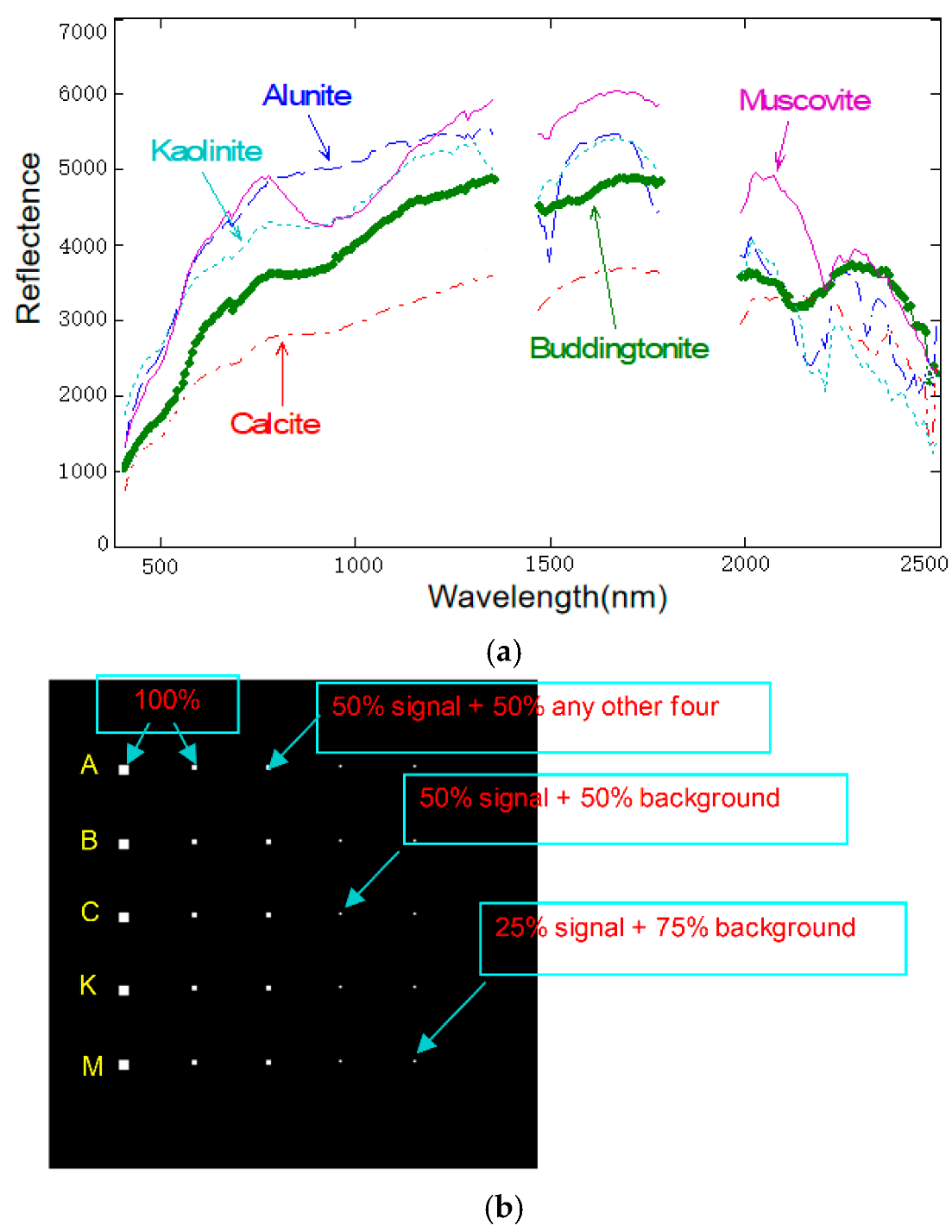
The synthetic dataset was simulated from real Nevada copper ore data on the USGS website, as shown in Figure 2. The image had 350 × 350 pixels of 224 bands, and the wavelength ranged from 270 nm to 2480 nm. The 270 nm–300 nm, 1295 nm–1404 nm and 1739 nm–1946 nm bands (channel numbers 1–3, 105–115 and 150–170) were removed due to the water absorption and low signal-to-noise ratio (SNR) of the bands, leaving 189 bands that could be used in the experiments. The five pure pixels in the ground truth provided were Alunite (A), Buddingtonite (B), Calcite (C), Kaolinite (K) and Muscovite (M). We assume the simulated pixels were mixed linearly. These five mineral signatures were located in five rows, respectively, linearly mixed with the background in varying percentages.
The first column contained five 4 × 4 pure panel pixels, the second column contained five 2 × 2 pure panel pixels, the third column contained five 2 × 2 mixed pixels, and the fourth and fifth columns contained five 1 × 1 sub-pixels. The pixels were mixed according to the way marked in the Figure 2b. So, there were a total of 100 pure pixels in the data (80 in the first column and 20 in the second column). We used the average value in the sample area of the original image as the background signature in the simulated image, polluted by a 50% signal-to-noise ratio Gaussian noise.
4.2.2. Hyperspectral Digital Imagery Collection Experiment (Hydice) Dataset
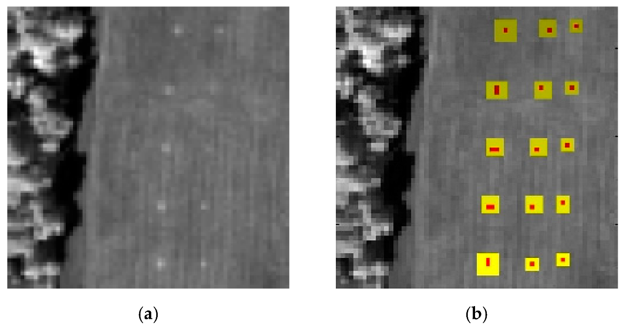
The Hydice real hyperspectral dataset, as shown in Figure 3, has 64 × 64 pixels. It has 210 bands ranging from 400 nm to 2500 nm, with a spectral resolution of 10 nm. After removing low-signal/high-noise bands 400 nm–430 nm and 2410 nm–2500 nm (band numbers 1–3 and 202–210), and water vapor absorption bands 1400 nm–1520 nm and 1750 nm–1930 nm (band numbers: 101–112 and 137–153), 169 bands were used in the experiments, as shown in Figure 3b, which contained 19-panel pixels. The panel pixel in the center is marked in red, and yellow represents the boundary pixel. There were five rows and three columns of panel pixels, all of which were single target pixels except the last four panel pixels in the first column, which contained two target pixels. In the study, the number p of target pixels generated by ATGP, VCA and SGA was estimated by virtual dimension to be 29 [38].
4.2.3. Samson Dataset
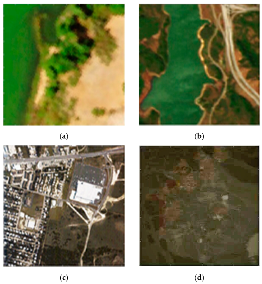
Samson is one of the commonly used hyperspectral datasets. Due to the computational cost problem caused by the large original image, it is usually intercepted for analysis. Starting from the (252,232) pixel, the sub-image contains 95 × 95 pixel of 156 bands, covering the wavelength range from 401 nm to 889 nm with spectral resolution of 3.13 nm. There are three endmembers corresponding to Soil, Tree and Water. The pseudo-color image is shown in Figure 4a.
4.2.4. Jasper Ridge Dataset
The Jasper Ridge dataset originally consisted of 512 × 614 pixels of 224 bands, covering the wavelength range from 380 nm to 2500 nm, with a spectral resolution of 9.46 nm. In addition, a sub-image of 100 × 100 pixels starting from the (105,269) pixel was used, as shown in Figure 4b. The 380 nm–408 nm, 1392 nm–1440 nm, 1827 nm–1950 nm and 2450 nm–2500 nm bands (band numbers 1–3, 108–112, 154–166 and 220–224) with dense water vapor and atmospheric effects were removed, and 198 bands were reserved for experimentation. There are four potential endmembers in this data: Road, Soil, Water and Tree.
4.2.5. Urban Dataset
Urban is one of the most widely used hyperspectral datasets in hyperspectral unmixing research. There are 307 rows and 307 columns of pixels, including 210 wavelengths ranging from 400 nm to 2500 nm, with a spectral resolution of 10 nm. Due to dense water vapor and atmospheric effects, wavelengths 400 nm–440 nm, 1150 nm–1160 nm, 1260 nm–1270 nm, 1400 nm–1510 nm, 1750 nm–1930 nm and 2370 nm–2500 nm (channels 1–4, 76, 87, 101–111, 136–153 and 198–210) were removed, and 162 channels were retained. The ground truth containing five endmembers was used in the experiment, including Asphalt, Grass, Tree, Roof and Dirt. The dataset is shown in Figure 4c.
4.2.6. Cuprite Dataset
The Cuprite dataset is another widely used dataset for hyperspectral unmixing research, covering the mining area in Nevada, USA. The dataset has an area of 250 × 190 pixels of 224 channels, ranging from 370 nm to 2480 nm. After removing the noise bands 370 nm–389 nm and 2442 nm–2480 nm(channels 1–2 and 221–224), and the water vapor absorption bands 1340 nm–1434 nm and 1755 nm–1943 nm (channels 104–113 and 148–167), 188 channels were retained, including 14 minerals. To avoid the subtle differences between the variants of similar minerals, we finally reduced the number of endmembers to 12, which are summarized as follows: “Alunite,” “Andradite,” “Buddingtonite,” “Dumortierite,” “Kaolinite1,” “Kaolinite2,” “Moscovite,” “Montmorillonite,” “Nontronite,” “Pyrope,” “Sphene” and “Chalcedony,” as shown in Figure 4d.
4.3. Experimental Results
4.3.1. Performance of Locating Endmembers
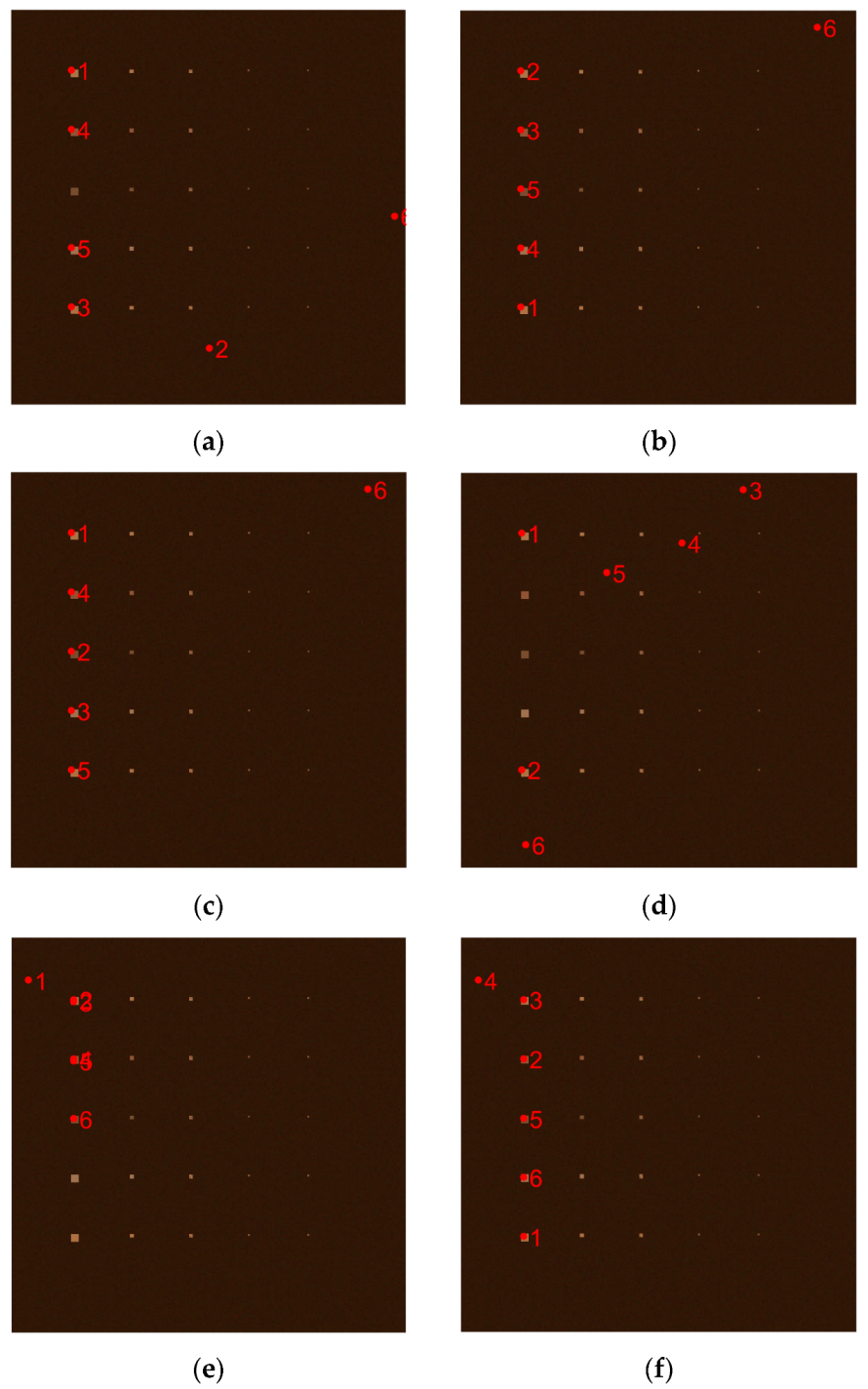
The experimental results on synthetic data are listed in Figure 5, where the extracted endmembers are located according to the position index, and the red solid dots are used to mark the location of the endmembers. The five-panel pixels in the first column of the synthetic dataset are all 4 × 4 in size, which meets the number of neighborhoods required for the calculation of spatial potential energy in the SPEW algorithm. In the process of spatial potential energy weighting, the center pixel of the uniform area is large. Therefore, SPEW succesfully found all types of pure pixels, as shown in Figure 5f, and the final position of the endmembers extracted by SPEW was in the middle of the pixel cluster, which is different from that of VCA, ATGP and SGA at the edge of each type of pure pixel panel. Among them, ATGP and SGA also extracted all types of pure pixels in the same position because these two algorithms are inherently equivalent under the same initial conditions. Meanwhile, the random initial condition of VCA made it unstable, and the algorithm failed to find all endmenbers corresponding to the five materials, as the endmember of Calcite was missed. The SENMAV algorithm extracted three valid endmembers when the balance parameter was adjusted to 0.3. ECSO also missed endmembers for Buddingtonite, Calcite and Kaolinite under spatial consideration.
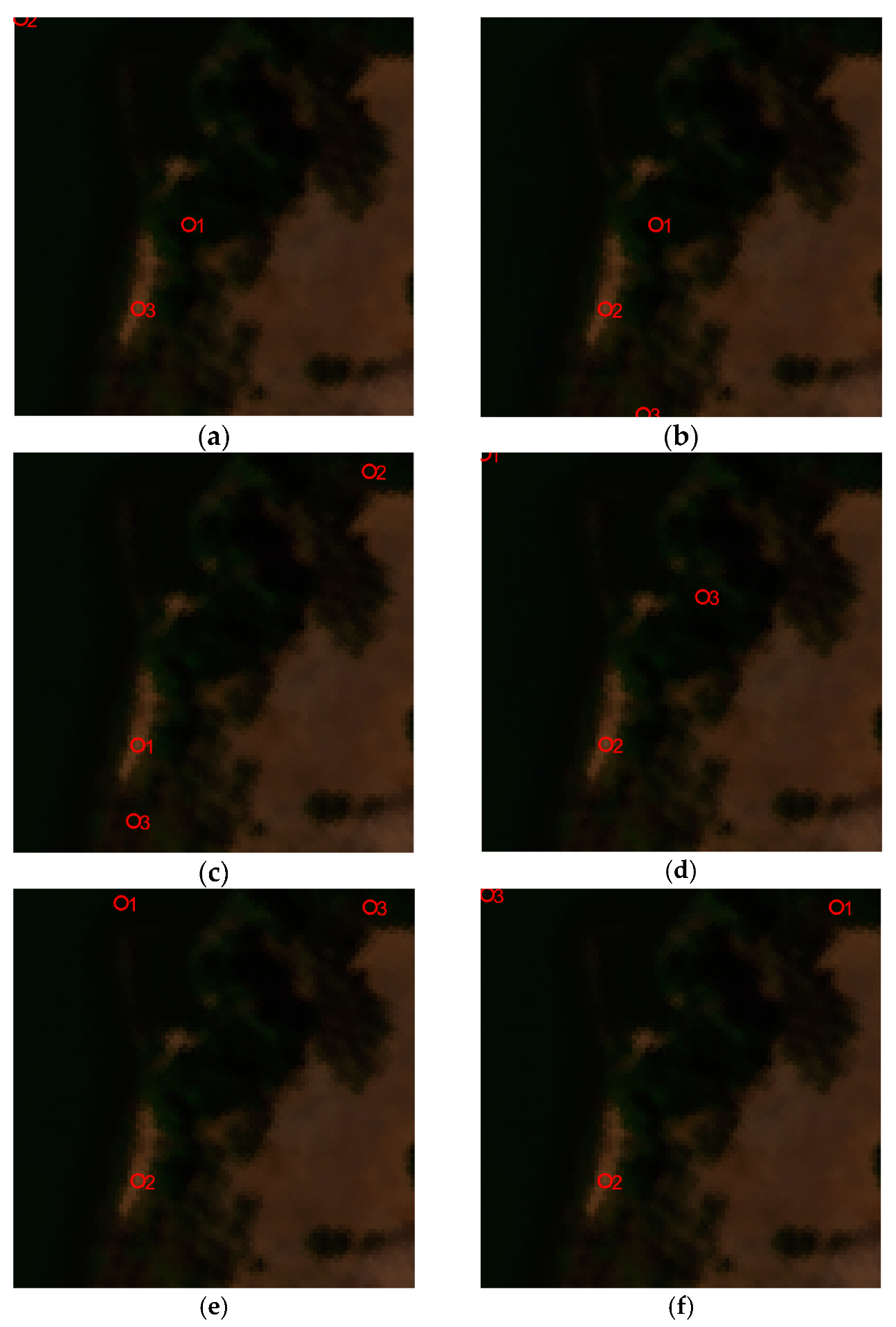
Furthermore, the Hydice dataset was used to test the endmember location performance for scattered endmembers. The target pixels in this dataset were single-pixel or dual-pixel, and the extraction of endmembers could not be restricted by spatial potential energy alone. As shown in Figure 6, VCA, ATGP, SGA and SPEW all achieved satisfatory results when the number of endmembers was determined as 29 by VD. However, SENMAV failed again to find all targets together with ECSO, which both utilized the spatial information. This can be attributed to the fact that for such small endmembers, neither entropy as spatial information nor space energy as constraint is effective. It is necessary to select representative pixels for them mainly accroding to the spectral character. The SPEW method makes up for the defect of the space potential energy method, which relies too heavily on the space neighborhood, where the spectral angle distance weight can be used to select some candidate endmembers for the scattered categories.
From the above results, it can be found that the SPEW may locate memebers more effectively with the central positon and the number of extracted endmembers corresponding to the disired materials.
4.3.2. Performance of Unmixing
The Samson dataset contained three endmembers, and the distribution was concentrated. Each endmember occupied a large proportion of the area where it was located. The three endmembers were partitioned. Therefore, the dataset clearly showed whether the extracted endmember positions were duplicated, which was very helpful for the subsequent quantitative analysis. As shown in Figure 7, the extraction positions of the three endmembers of the VCA, ECSO, SEMAV and SPEW algorithms were in three regions, respectively. However, ATGP and SAG had two endmembers located in the same area, which was the main reason for the following excessive reconstruction error.
The abundance map was sequentially obtained by the fully constrained least squares (FCLS) algorithm with the extracted endmembers of SPEW, SENMAV, VCA, ATGP and SGA. The RMSE between the estimated abundance vector and ground-truth abundance vector, the SAD value between the extracted endmembers and the ground-truth endmembers, and the RE between the reconstruction data and the original data were calculated for comparison in Table 1. In the table, the optimal value is in bold and underlined, and the suboptimal value is in bold. The results show that the SPEW algorithm provided the best average SAD, espacially the SAD on Water. As for the RMSE and RE, our algorithm achieved the second best performance. In addition, Table 1 clearly shows that the Water endmember found by ATGP and SGA was far away from the Tree endmember, which led to the large RMSE and RE of these two algorithms.
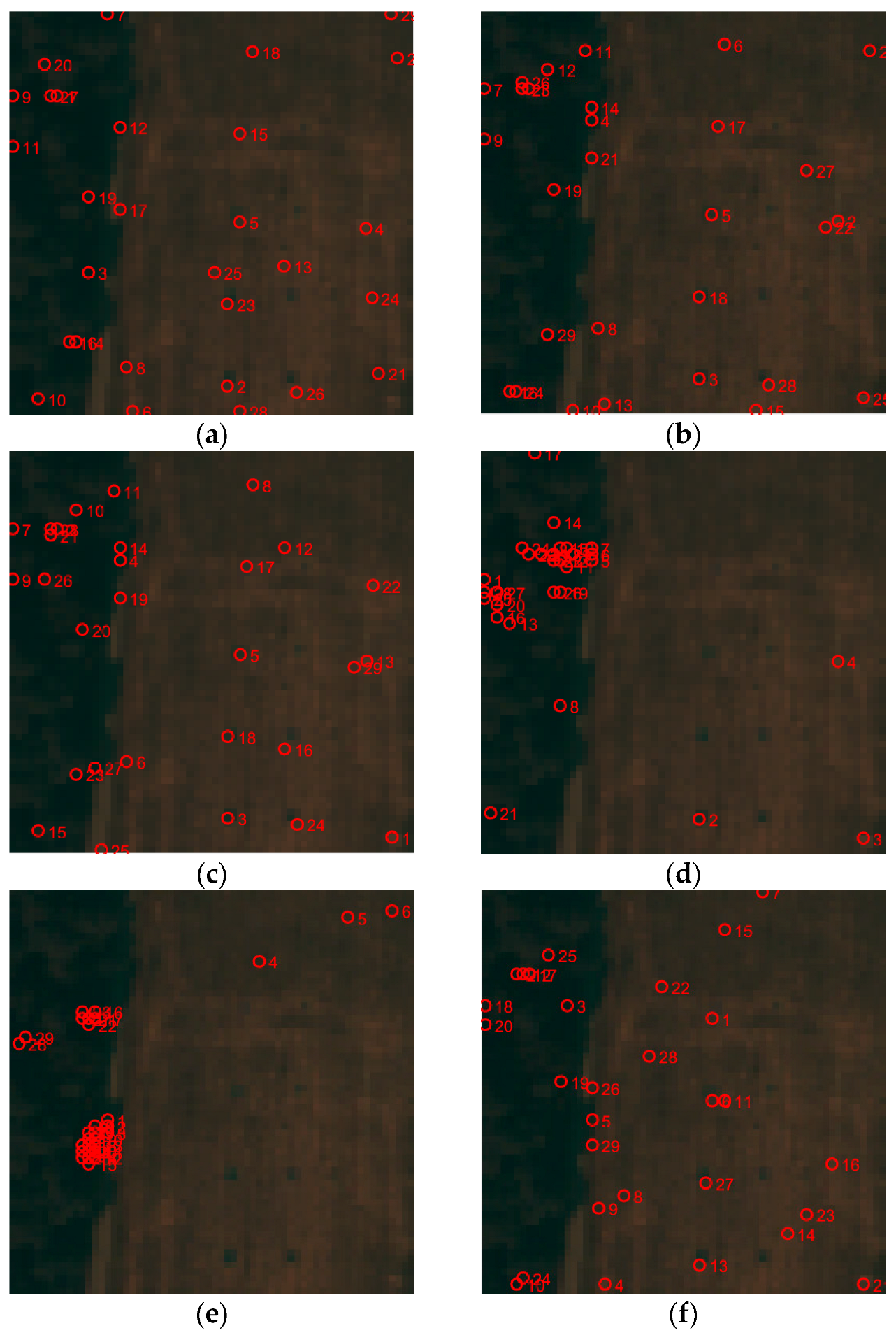
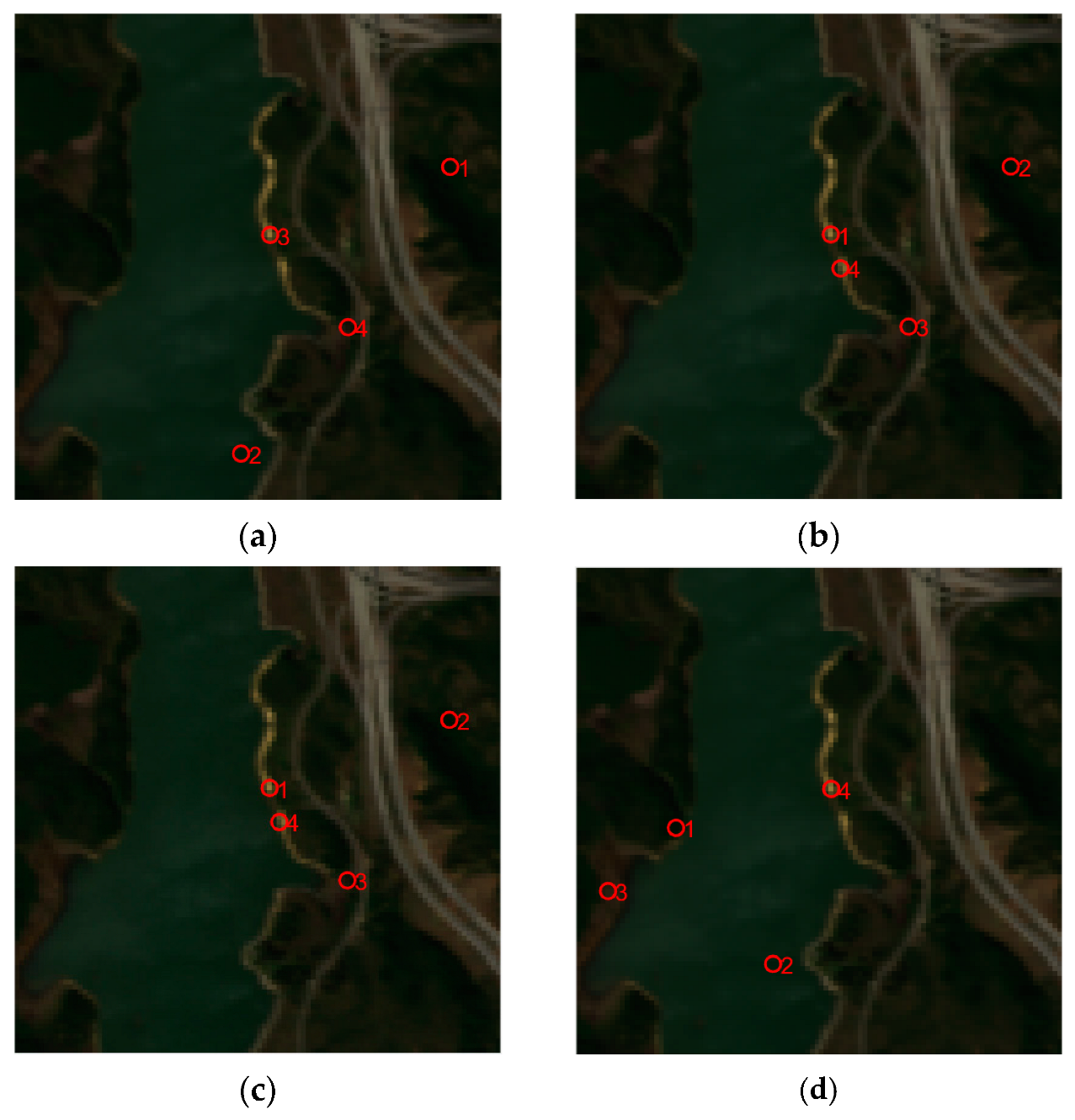
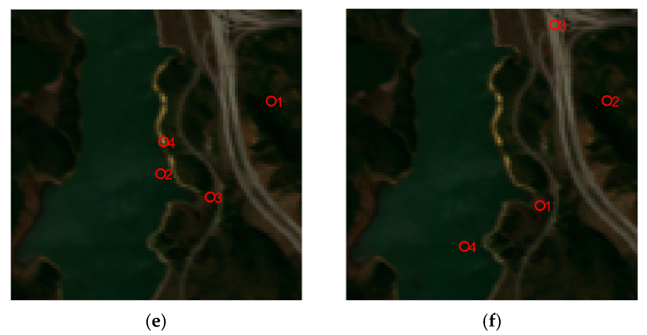
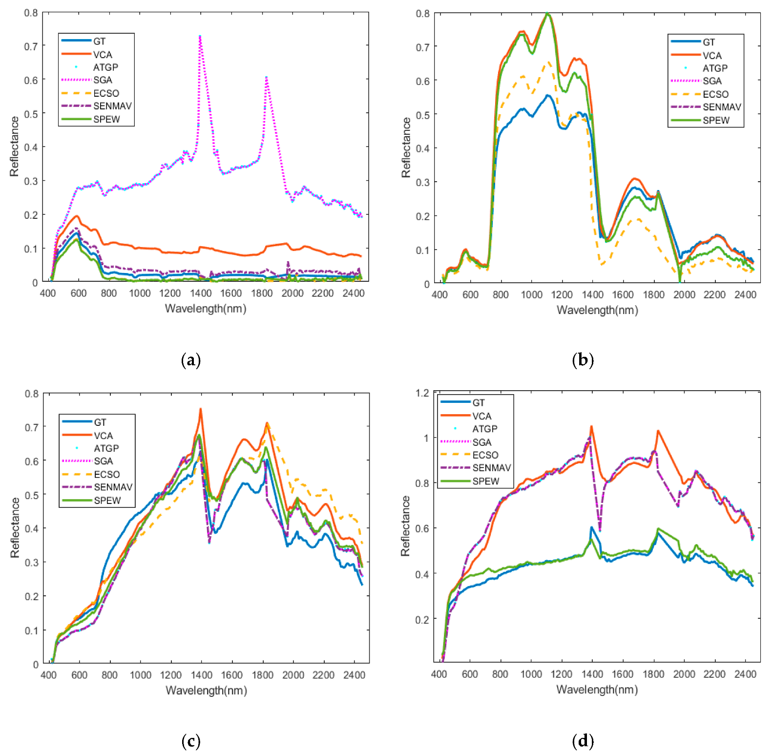
The endmember extraction results on the Jasper Ridge dataset are shown in Figure 8, where four endmembers are desired. In the dataset, the Road class was small, but it was continuous and long across the image. As shown in Figure 8, the locations of the ATGP and SGA endmembers were similar because these two algorithms were the same when the first two endmembers are initialized identically. In Figure 8f, the location of the Road endmember extracted by SPEW was clearly different from that of other algorithms. Therefore, we intuitively compared the performance of each algorithm through the extracted endmember spectrum in Figure 9. According to the reflectance curves extracted by the SPEW algorithm for the four endmembers of Jasper Ridge, the curve shape and reflectance value of the Road endmember showed the best consistancy with the ground truth.
Table 2 lists unmixing performance of the tested algorithms on the Jasper Ridge dataset. Among them, SPEW showed the best average SAD, RMSE and RE, especially on the SAD of the Road endmember. This indicates that the spectrum found by SPEW for Road is more accurate than the other algorithms.
On the Urban dataset, all algorithms may extract valid endmembers and provide equivalent unmixing performance, as shown in Table 3. Although the SENMAV algorithm obtained the smallest RMSE, the SPEW showed advantages on both the mean SAD and RE, and ranked second on the RMSE following SENMAV.
Since the Cuprite dataset did not have ground truth abundances, the RMSE and RE could not be calculated, and only the analysis of the SAD is provided here. According to Table 4, among the 12 endmembers in the dataset, the Buddingtonite, Kaolinite_2, Muscovite, Montmorillonite and Sphene endmembers extraced by SPEW had the smallest SAD, which means they were closest to the true spectrum. Moreover, the average SAD was only larger than that of the VCA, but better than the other four algorithms.
5. Discussion
According to the above experimental results, compared with VCA, ATGP and SGA only using spectral information to extract endmembers, the SPEW algorithm essentially has a smaller spectral angle distance, abundance error and reconstruction error because the weight of space potential energy can suppress the influence of noise and anomaly. Thus, the possibility of uniform region endmember extraction is improved. On the other hand, when compared with ECSO and SENMAV using spatial information, SPEW algorithm can find discrete representative endmembers with the weighting of the spectral angle distance, making up for the defect of space constraint. Therefore, the SPEW algorithm holds great potential for wide application.
For the clustering numerical estimation problem of K-means clustering, experiments were performed on the Cuprite dataset, as discussed by the authors of [30]. The conclusion is that better performance can be achieved when the number of clusters is 2p. The SPEW algorithm obtains the classification labels through the clustering method, and then calculates the spatial potential energy of the pixels according to the classification labels. The purpose is to find the pixels located in the spatially uniform area as the candidate endmembers. From the experimental results, the unsupervised clustering method K-means can achieve our goal of suppressing noise and anomalies.
In order to automatically weight candidate endmembers according to the spectral angular distance, the OTSU method was used to divide the large spectral angular distance from the small spectral angular distance. This method can perform more accurate and reasonable segmentation when the spectral angular distances of the pixels are similar.
6. Conclusions
In this paper, we proposed a spatial potential energy weighted maximum simplex algorithm (SPEW) for hyperspectral endmember extraction. First, it overcomes the problem of SENMAV on adjusting the balance parameters. Second, it makes up for the problem of algorithms with spatial constraint, which only identify endmembers in spatially uniform regions. In our algorithm, the spatial potential energy of each pixel is used to give a large weight to the pixels in a spatially uniform region, and the spectral angle distance method is used to give large weights to the representative pixels for the scattered small-class pixels. Finally, the weighted pixels constituting the maximum simplex are selected as the endmembers. The SPEW does not rely on any parameters and can automatically evaluate the endmembers comprehensively. It can be concluded from the experiment that the SPEW algorithm combines spectral characteristics and spatial characteristics well, increases the accuracy of endmember extraction compared to traditional algorithms and defeats the other spatial algorithms on finding the endmember for small scattered areas. Consequently, the SPEW algorithm has the best overall performance.
Although our algorithm has a high accuracy, it consumes a lot of time. It is our future research content to further speed up the algorithm.
Author Contributions
Conceptualization, M.S. and Y.L.; formal analysis, M.S.; methodology, Y.L. and T.Y.; writing—original draft preparation, M.S. and Y.L; writing—review and editing, T.Y. and D.X. All authors have read and agreed to the published version of the manuscript.
Funding
This work was supported by the National Natural Science Foundation of China under Grant No. 61971082, No. 61890964, and No. 61601077.
Institutional Review Board Statement
Not applicable.
Informed Consent Statement
Not applicable.
Conflicts of Interest
The authors declare no conflict of interest.
References
- Bioucas-Dias, J.M.; Plaza, A.; Camps-Valls, G.; Scheunders, P.; Nasrabadi, N.M.; Chanussot, J. Hyperspectral remote sensing data analysis and future challenges. IEEE Geosci. Remote Sens. Mag. 2013, 1, 6–36. [Google Scholar] [CrossRef] [Green Version]
- Xu, X.; Li, J.; Li, S.; Plaza, A. Generalized Morphological Component Analysis for Hyperspectral Unmixing. IEEE Trans. Geosci. Remote Sens. 2020, 58, 2817–2832. [Google Scholar] [CrossRef]
- Brown, A.J.; Hook, S.J.; Baldridge, A.M.; Crowley, J.K.; Bridges, N.T.; Thomson, B.J.; Marion, G.M.; Filho, C.R.D.S.; Bishop, J.L. Hydrothermal formation of Clay-Carbonate alteration assemblages in the Nili Fossae region of Mars. Earth Planet. Sci. Lett. 2010, 297, 174–182. [Google Scholar] [CrossRef] [Green Version]
- Chang, C.I.; Wen, C.H.; Wu, C.C. Relationship exploration among PPI, ATGP and VCA via theoretical analysis. Int. J. Comput. Sci. Eng. 2013, 8, 361–367. [Google Scholar] [CrossRef]
- Ren, H.; Chang, C.-I. Automatic spectral target recognition in hyperspectral imagery. IEEE Trans. Aerosp. Electron. Syst. 2003, 39, 1232–1249. [Google Scholar] [CrossRef] [Green Version]
- Nascimento, J.M.; Dias, J.M. Vertex component analysis: A fast algorithm to unmix hyperspectral data. IEEE Trans. Geosci. Remote Sens. 2005, 43, 898–910. [Google Scholar] [CrossRef] [Green Version]
- Winter, M.E. N-finder: An algorithm for fast autonomous spectral endmember determination in hyperspectral data. In Proceedings of the SPIE′s International Symposium on Optical Science, Engineering, and Instrumentation, Denver, CO, USA, 18–23 July 1999; International Society for Optics and Photonics: Bellingham, WA, USA, 1999; Volume 3753, pp. 266–276. [Google Scholar]
- Xiong, W.; Chang, C.-I.; Wu, C.-C.; Kalpakis, K.; Chen, H.M. Fast Algorithms to Implement N-FINDR for Hyperspectral Endmember Extraction. IEEE J. Sel. Top. Appl. Earth Obs. Remote Sens. 2011, 4, 545–564. [Google Scholar] [CrossRef]
- Chang, C.-I.; Wu, C.-C.; Liu, W.-M.; Ouyang, Y.-C. A New Growing Method for Simplex-Based Endmember Extraction Algorithm. IEEE Trans. Geosci. Remote Sens. 2006, 44, 2804–2819. [Google Scholar] [CrossRef]
- Shi, Y.; Wang, H.; Guo, X.; Xu, G. Endmember Extraction Using Minimum Volume and Information Constraint Nonnegative Matrix Factorization. IEEE Geosci. Remote Sens. Lett. 2019, 16, 1427–1431. [Google Scholar] [CrossRef]
- Miao, L.; Qi, H. Endmember Extraction From Highly Mixed Data Using Minimum Volume Constrained Nonnegative Matrix Factorization. IEEE Trans. Geosci. Remote Sens. 2007, 45, 765–777. [Google Scholar] [CrossRef]
- Qian, Y.; Jia, S.; Zhou, J.; Robles-Kelly, A. Hyperspectral unmixing via L1/2 sparsity-constrained nonnegative matrix fac-torization. IEEE Trans. Geosci. Remote Sens. 2011, 49, 4282–4297. [Google Scholar] [CrossRef] [Green Version]
- Parente, M.; Clark, J.T.; Brown, A.J.; Bishop, J. End-to-End Simulation and Analytical Model of Remote-Sensing Systems: Application to CRISM. IEEE Trans. Geosci. Remote Sens. 2010, 48, 3877–3888. [Google Scholar] [CrossRef]
- Mei, S.; He, M.; Wang, Z.; Feng, D. Spatial Purity Based Endmember Extraction for Spectral Mixture Analysis. IEEE Trans. Geosci. Remote Sens. 2010, 48, 3434–3445. [Google Scholar] [CrossRef]
- Li, H.; Zhang, L. A Hybrid Automatic Endmember Extraction Algorithm Based on a Local Window. IEEE Trans. Geosci. Remote Sens. 2011, 49, 4223–4238. [Google Scholar] [CrossRef]
- Xu, M.; Du, B.; Zhang, L. Spatial-Spectral Information Based Abundance-Constrained Endmember Extraction Methods. IEEE J. Sel. Top. Appl. Earth Obs. Remote Sens. 2014, 7, 2004–2015. [Google Scholar] [CrossRef]
- Madronero, M.T.; Velez-Reyes, M. Integrating Spatial Information in Unsupervised Unmixing of Hyperspectral Imagery Using Multiscale Representation. IEEE J. Sel. Top. Appl. Earth Obs. Remote Sens. 2014, 7, 1985–1993. [Google Scholar] [CrossRef]
- Xu, M.; Zhang, L.; Du, B. An image-based endmember bundle extraction algorithm using both spatial and spectral in-formation. IEEE J. Sel. Topics Appl. Earth Observ. Remote Sens. 2015, 8, 2607–2617. [Google Scholar] [CrossRef]
- Wang, L.; Shi, C.; Diao, C.; Ji, W.; Yin, D. A survey of methods incorporating spatial information in image classification and spectral unmixing. Int. J. Remote Sens. 2016, 37, 3870–3910. [Google Scholar] [CrossRef]
- Shen, X.; Bao, W.; Qu, K. Clustering based spatial spectral preprocessing for hyperspectral unmxing. In Proceedings of the 4th International Conference on Communication and Information Processing—ICCIP’ 18, Qingdao, China, 2–4 November 2018; Association for Computing Machinery (ACM): New York, NY, USA; pp. 313–316. [Google Scholar]
- Shen, X.; Bao, W. A Spatial Energy And Spectral Purity Based Preprocessing Algorithm For Fast Hyperspectral Endmember Extraction. In Proceedings of the 2019 10th Workshop on Hyperspectral Imaging and Signal Processing: Evolution in Remote Sensing (WHISPERS), Amsterdam, The Netherlands, 24–26 September 2019; Institute of Electrical and Electronics Engineers (IEEE): Piscataway, NJ, USA; pp. 1–5. [Google Scholar]
- Shen, X.; Bao, W. Hyperspectral Endmember Extraction Using Spatially Weighted Simplex Strategy. Remote Sens. 2019, 11, 2147. [Google Scholar] [CrossRef] [Green Version]
- Yan, Y.; Hua, W.; Liu, X.; Cui, Z.; Diao, D. Spatial–spectral preprocessing for spectral unmixing. Int. J. Remote Sens. 2018, 40, 1357–1373. [Google Scholar] [CrossRef]
- Plaza, A.; Martinez, P.; Perez, R.; Plaza, J. Spatial/spectral endmember extraction by multidimensional morphological operations. IEEE Trans. Geosci. Remote Sens. 2002, 40, 2025–2041. [Google Scholar] [CrossRef] [Green Version]
- Zortea, M.; Plaza, A. Spatial Preprocessing for Endmember Extraction. IEEE Trans. Geosci. Remote Sens. 2009, 47, 2679–2693. [Google Scholar] [CrossRef]
- Martín, G.; Plaza, A. Region-Based Spatial Preprocessing for Endmember Extraction and Spectral Unmixing. IEEE Geosci. Remote Sens. Lett. 2011, 8, 745–749. [Google Scholar] [CrossRef] [Green Version]
- Martín, G.; Plaza, A. Spatial-Spectral Preprocessing Prior to Endmember Identification and Unmixing of Remotely Sensed Hyperspectral Data. IEEE J. Sel. Top. Appl. Earth Obs. Remote Sens. 2012, 5, 380–395. [Google Scholar] [CrossRef]
- Mei, S.; Zhang, G.; Li, J.; Zhang, Y.; Du, Q. Improving Spectral-Based Endmember Finding by Exploring Spatial Context for Hyperspectral Unmixing. IEEE J. Sel. Top. Appl. Earth Obs. Remote Sens. 2020, 13, 3336–3349. [Google Scholar] [CrossRef]
- Shah, D.; Zaveri, T.; Trivedi, Y.N.; Plaza, A. Entropy-Based Convex Set Optimization for Spatial–Spectral Endmember Extraction From Hyperspectral Images. IEEE J. Sel. Top. Appl. Earth Obs. Remote Sens. 2020, 13, 4200–4213. [Google Scholar] [CrossRef]
- Shen, X.; Bao, W.; Qu, K. Spatial-Spectral Hyperspectral Endmember Extraction Using a Spatial Energy Prior Constrained Maximum Simplex Volume Approach. IEEE J. Sel. Top. Appl. Earth Obs. Remote Sens. 2020, 13, 1347–1361. [Google Scholar] [CrossRef]
- Tarabalka, Y.; Fauvel, M.; Chanussot, J.; Benediktsson, J.A. SVM- and MRF-Based Method for Accurate Classification of Hyperspectral Images. IEEE Geosci. Remote Sens. Lett. 2010, 7, 736–740. [Google Scholar] [CrossRef] [Green Version]
- Khodadadzadeh, M.; Li, J.; Plaza, A.; Ghassemian, H.; Bioucas-Dias, J.M.; Li, X. pectral-spatial classification of hyper-spectral data using local and global probabilities for mixed pixel characterization. IEEE Trans. Geosci. Remote Sens. 2014, 52, 6298–6314. [Google Scholar] [CrossRef]
- Xia, J.; Chanussot, J.; Du, P.; He, X. Spectral–Spatial Classification for Hyperspectral Data Using Rotation Forests With Local Feature Extraction and Markov Random Fields. IEEE Trans. Geosci. Remote Sens. 2014, 53, 2532–2546. [Google Scholar] [CrossRef]
- Eches, O.; Dobigeon, N.; Tourneret, J.-Y. Enhancing Hyperspectral Image Unmixing With Spatial Correlations. IEEE Trans. Geosci. Remote Sens. 2011, 49, 4239–4247. [Google Scholar] [CrossRef] [Green Version]
- Li, W.; Prasad, S.; Fowler, J.E. Hyperspectral Image Classification Using Gaussian Mixture Models and Markov Random Fields. IEEE Geosci. Remote Sens. Lett. 2014, 11, 153–157. [Google Scholar] [CrossRef] [Green Version]
- Du, Q.; Raksuntorn, N.; Younan, N.H.; King, R.L. End-member extraction for hyperspectral image analysis. Appl. Opt. 2008, 47, F77–F84. [Google Scholar] [CrossRef] [PubMed]
- Hartigan, J.A.; Wong, M.A. Algorithm AS 136: A K-Means Clustering Algorithm. J. R. Stat. Soc. Ser. (Appl. Stat.) 1979, 28, 100–108. [Google Scholar] [CrossRef]
- Chang, C.-I.; Chen, S.-Y.; Li, H.-C.; Chen, H.-M.; Wen, C.-H. Comparative Study and Analysis Among ATGP, VCA, and SGA for Finding Endmembers in Hyperspectral Imagery. IEEE J. Sel. Topics Appl. Earth Observ. Remote Sen. 2016, 9, 4280–4306. [Google Scholar] [CrossRef]
Figure 1.
Framework of the proposed SPEW algorithm.

Figure 2.
(a) Five mineral reflectance spectra. (b) A set of 25 panels simulated by A, B, C, K and M.
Figure 2.
(a) Five mineral reflectance spectra. (b) A set of 25 panels simulated by A, B, C, K and M.

Figure 3.
(a) Hydice panel scene with 15 panels. (b) Locations of the 15 panels.

Figure 4.
Pseudo-color map of the datasets: (a) Samson, (b) Jasper Ridge, (c) Urban, (d) Cuprite.

Figure 5.
Endmember location maps on the synthetic dataset: (a) VCA, (b) ATGP, (c) SGA, (d) ECSO, (e) SENMAV, (f) SPEW.
Figure 5.
Endmember location maps on the synthetic dataset: (a) VCA, (b) ATGP, (c) SGA, (d) ECSO, (e) SENMAV, (f) SPEW.

Figure 6.
Endmember location maps on the Hydice dataset: (a) VCA, (b) ATGP, (c) SGA, (d) ECSO, (e) SENMAV, (f) SPEW.
Figure 6.
Endmember location maps on the Hydice dataset: (a) VCA, (b) ATGP, (c) SGA, (d) ECSO, (e) SENMAV, (f) SPEW.

Figure 7.
Estimated endmember location maps on the Samson dataset: (a) VCA, (b) ATGP, (c) SGA, (d) ECSO, (e) SENMAV, (f) SPEW.
Figure 7.
Estimated endmember location maps on the Samson dataset: (a) VCA, (b) ATGP, (c) SGA, (d) ECSO, (e) SENMAV, (f) SPEW.

Figure 8.
Endmember location maps on the Jasper Ridge dataset: (a) VCA, (b) ATGP, (c) SGA, (d) ECSO, (e) SENMAV, (f) SPEW.
Figure 8.
Endmember location maps on the Jasper Ridge dataset: (a) VCA, (b) ATGP, (c) SGA, (d) ECSO, (e) SENMAV, (f) SPEW.


Figure 9.
Comparison between the estimated and ground-truth endmember spectral signatures: (a) Soil, (b) Tree, (c) Water, (d) Road.
Figure 9.
Comparison between the estimated and ground-truth endmember spectral signatures: (a) Soil, (b) Tree, (c) Water, (d) Road.


Table 1.
SAD, RMSE and RE of all test algorithms on the Samson dataset.
| Algorithms | VCA | ATGP | SGA | ECSO | SENMAV | SPEW |
|---|---|---|---|---|---|---|
| Soil | 0.0399 | 0.0219 | 0.0407 | 0.0404 | 0.0404 | 0.1224 |
| Tree | 0.0236 | 0.0404 | 0.0404 | 0.0713 | 0.0407 | 0.0407 |
| Water | 0.1504 | 1.0948 | 1.1483 | 0.1553 | 0.1296 | 0.0404 |
| Mean | 0.0713 | 0.3857 | 0.4098 | 0.0890 | 0.0702 | 0.0678 |
| RMSE | 0.3253 | 0.3359 | 0.3689 | 0.2733 | 0.3237 | 0.3233 |
| RE | 0.0014 | 0.2421 | 0.2429 | 0.0057 | 0.0028 | 0.0020 |
Table 2.
SAD, RMSE and RE of all test algorithms on the Jasper Ridge dataset.
| Algorithms | VCA | ATGP | SGA | ECSO | SENMAV | SPEW |
|---|---|---|---|---|---|---|
| Soil | 0.1481 | 0.1069 | 0.1180 | 0.2030 | 0.2652 | 0.1233 |
| Tree | 0.2554 | 0.1159 | 0.1069 | 0.2540 | 0.1559 | 0.2543 |
| Water | 0.0901 | 0.1336 | 0.1336 | 0.1961 | 0.1069 | 0.1559 |
| Road | 0.1166 | 0.8953 | 0.8953 | 0.1069 | 0.1336 | 0.0443 |
| Mean | 0.1525 | 0.3129 | 0.3134 | 0.1900 | 0.1654 | 0.1444 |
| RMSE | 0.1560 | 0.2190 | 0.2324 | 0.1350 | 0.1612 | 0.1257 |
| RE | 0.0207 | 0.3104 | 0.3148 | 0.0074 | 0.0069 | 0.0048 |
Table 3.
SAD, RMSE and RE of all test algorithms on the Urban dataset.
| Algorithms | VCA | ATGP | SGA | ECSO | SENMAV | SPEW |
|---|---|---|---|---|---|---|
| Asphalt | 0.1416 | 0.1227 | 0.0798 | 0.1227 | 0.1740 | 0.3069 |
| Grass | 0.1517 | 0.1462 | 0.1227 | 0.1740 | 0.1160 | 0.1587 |
| Tree | 1.1779 | 0.1480 | 0.2112 | 0.3893 | 1.1990 | 1.0581 |
| Roof | 0.1388 | 0.5432 | 0.5432 | 0.8092 | 0.1956 | 0.0741 |
| Dirt | 0.1127 | 1.3748 | 1.3748 | 1.1410 | 0.1227 | 0.1062 |
| Mean | 0.3445 | 0.4669 | 0.4663 | 0.5272 | 0.3615 | 0.3408 |
| RMSE | 0.3288 | 0.3272 | 0.3244 | 0.3331 | 0.2789 | 0.3158 |
| RE | 0.1362 | 0.2792 | 0.2792 | 0.1358 | 0.1658 | 0.0162 |
Table 4.
SAD of all test algorithms on the Cuprite dataset.
| Algorithms | VCA | ATGP | SGA | ECSO | SENMAV | SPEW |
|---|---|---|---|---|---|---|
| Alunite | 0.0962 | 0.0824 | 0.9675 | 0.9543 | 0.0889 | 0.1413 |
| Andradite | 0.0691 | 1.1329 | 0.0824 | 0.1046 | 0.0797 | 1.0480 |
| Buddingtonite | 0.0896 | 0.0848 | 0.0848 | 0.1150 | 0.1114 | 0.0622 |
| Dumortierite | 0.8286 | 0.0859 | 0.0859 | 0.0892 | 0.0948 | 0.1895 |
| Kaolinite_1 | 0.0838 | 0.0618 | 0.0618 | 0.0701 | 0.0603 | 0.0743 |
| Kaolinite_2 | 0.1133 | 0.1159 | 0.1159 | 0.1702 | 0.1982 | 0.0824 |
| Muscovite | 0.0741 | 0.0736 | 0.0736 | 0.0859 | 0.1195 | 0.0704 |
| Montmorillonite | 0.1500 | 0.2400 | 0.1695 | 0.1204 | 1.0240 | 0.0812 |
| Nontronite | 0.0615 | 0.0802 | 0.0802 | 0.2337 | 0.1057 | 0.1604 |
| Pyrope | 0.1248 | 0.0852 | 0.0852 | 1.1614 | 0.0680 | 0.0998 |
| Sphene | 0.0797 | 0.1207 | 0.1027 | 1.1696 | 0.0736 | 0.0734 |
| Chalcedony | 0.0583 | 0.0994 | 0.8724 | 1.1330 | 0.9396 | 0.0704 |
| Mean | 0.1524 | 0.1886 | 0.2318 | 0.4506 | 0.2467 | 0.1794 |
Publisher’s Note: MDPI stays neutral with regard to jurisdictional claims in published maps and institutional affiliations. |
© 2022 by the authors. Licensee MDPI, Basel, Switzerland. This article is an open access article distributed under the terms and conditions of the Creative Commons Attribution (CC BY) license (https://creativecommons.org/licenses/by/4.0/).
Share and Cite
MDPI and ACS Style
Song, M.; Li, Y.; Yang, T.; Xu, D. Spatial Potential Energy Weighted Maximum Simplex Algorithm for Hyperspectral Endmember Extraction. Remote Sens. 2022, 14, 1192. https://doi.org/10.3390/rs14051192
AMA Style
Song M, Li Y, Yang T, Xu D. Spatial Potential Energy Weighted Maximum Simplex Algorithm for Hyperspectral Endmember Extraction. Remote Sensing. 2022; 14(5):1192. https://doi.org/10.3390/rs14051192
Chicago/Turabian StyleSong, Meiping, Ying Li, Tingting Yang, and Dayong Xu. 2022. "Spatial Potential Energy Weighted Maximum Simplex Algorithm for Hyperspectral Endmember Extraction" Remote Sensing 14, no. 5: 1192. https://doi.org/10.3390/rs14051192
Note that from the first issue of 2016, this journal uses article numbers instead of page numbers. See further details here.