
Accurate Monitoring of Submerged Aquatic Vegetation in a Macrophytic Lake Using Time-Series Sentinel-2 Images


1
College of Resources, Environment and Tourism, Capital Normal University, Beijing 100048, China
2
Beijing Municipal Key Lab of Resources Environment and GIS, Beijing 100048, China
3
College of Geospatial Information Science and Technology, Capital Normal University, Beijing 100048, China
*
Author to whom correspondence should be addressed.
Remote Sens. 2022, 14(3), 640; https://doi.org/10.3390/rs14030640
Submission received: 15 December 2021
/
Revised: 18 January 2022
/
Accepted: 23 January 2022
/
Published: 28 January 2022
(This article belongs to the Special Issue Remote Sensing of Floodplain Rivers and Freshwater Ecosystems)
Abstract
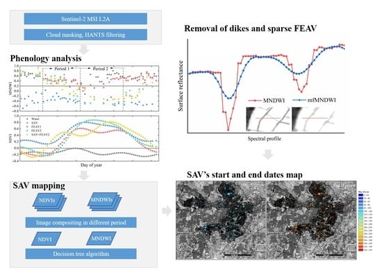
:Submerged aquatic vegetation (SAV) is one of the most important biological groups in shallow lakes ecosystems, and it plays a vital role in stabilizing the structure and function of water ecosystems. The study area of this research is Baiyangdian, which is a typical macrophytic lake with complex land cover types. This research aims to solve the low accuracy problem of the remote sensing extraction of SAV, which is mainly caused by water level fluctuations, differences in life-history characteristics, and mixed-pixel phenomena. Here, we developed a phenology–pixel method to determine the spatial distribution of SAV and the start and end dates of its growing season by using all Sentinel-2 images collected over a year on the Google Earth Engine platform. The experimental results show the following: (1) The phenology–pixel algorithm can effectively identify the maximum spatial distribution and growth period of submerged aquatic vegetation in Baiyangdian Lake throughout the year. The unique normalized difference vegetation index (NDVI) peak characteristics of Potamogeton crispus from March to May were used to effectively distinguish it from the low Phragmites australis population. Textural features based on the modified normalized difference water index (MNDWI) index effectively removed the mixed-pixel phenomenon of macrophytic lakes (such as dikes and sparse reeds). (2) A complete five-day interval NDVI time-series dataset was obtained, which removes potential noise on the temporal scale and fills in noisy observations by the harmonic analysis of time series (HANTS) method. We determined the two phenological periods of typical SAV by analyzing the intrayear variation characteristics of NDVI and MNDWI. (3) Using field-survey data for accuracy verification, the overall accuracy of our method was determined to be 94.8%, and the user’s accuracy and producer’s accuracy were 93.3% and 87.3%, respectively. Determining the temporal and spatial distribution of different SAV populations provides important technical support for actively promoting the maintenance and reconstruction of lake and reservoir ecosystems.
1. Introduction
As an important part of the lake ecosystem, wetland aquatic vegetation can change the physical and chemical environment of lake water bodies [1]. Aquatic vegetation serves important ecological and environmental purposes, such as providing habitat for species, stabilizing sediments, regulating nutrient circulation, and improving water quality [2,3,4,5,6]. Therefore, it plays a critical role in the evolution and ecological balance of lakes. Aquatic macrophytes in inland lakes can be divided into three categories, namely emergent aquatic vegetation, floating aquatic vegetation, and submerged aquatic vegetation (SAV). SAV is related to water transparency, water depth, and eutrophication, and its biomass is usually considered a key indicator for evaluating the quality of inland shallow lake ecosystems [7]. The distribution of aquatic macrophytes directly affects the habitat quality of the lake ecosystem, especially SAV, which can cause the aquatic ecosystem to change from a turbid algae-dominated state to a clear-water plant-dominated state [8,9]. Therefore, determining the distribution and growth duration of SAV can provide useful information for lake management and future ecological restoration.
Traditional monitoring methods for SAV are often limited by the water environment and high cost, resulting in a small monitoring range and destructive effects on SAV [10]. In addition, limited field-survey data may not be able to represent the spatial and temporal dynamics of SAV in a lake. Therefore, remote sensing technology has become an effective tool for mapping SAV [11]. Recently, multispectral sensor data have seen wide usage in mapping the distribution of large-scale aquatic vegetation and in evaluating the intra-annual and interannual variation of aquatic vegetation [9,12].
Generally speaking, a specific band or combination of bands (spectral index) can be used to distinguish between lake water bodies and aquatic vegetation, so multispectral sensor data have been widely used in the remote sensing extraction of aquatic vegetation [13]. For example, Dehua et al. [14] and Luo et al. [15] respectively used Landsat TM and HJ-CCD images to propose a decision tree model for identifying emergent aquatic vegetation, floating aquatic vegetation, and SAV in Taihu Lake. Brooks et al. [16] developed an algorithm based on the Landsat satellite to obtain the SAV maps of the Laurentian Great Lakes in the United States. Based on the uncertainty of the extraction threshold of SAV under different lakes and water quality conditions, Dai et al. [17] proposed a set of automatic threshold methods for extracting SAV from lakes on the Yangtze Plain of China and obtained good classification accuracy. Therefore, multispectral remote sensing data can be used to accurately survey and identify SAV in shallow lakes. The theoretical basis of these methods lies in the spectral difference between SAV, FEAV (floating leaves and emergent aquatic vegetation), and lake water.
Some studies have shown that the strong absorption of near-infrared makes it impossible to reflect the spectral information of SAV when the canopy depth is greater than 0.35 m [17,18]. However, the water level of inland lakes varies greatly during the year, making it difficult to detect when the distance between the vegetation canopy and the water surface is large. Theoretically, the growth position of SAV is roughly stable due to the vegetation’s strong roots. However, the turning of bottom silt caused by human activities or natural factors will increase the concentration of suspended sediment and decrease the light transmittance, which will hinder the accuracy of remote sensing detection. Therefore, previous studies have found that the area of SAV fluctuates greatly during the year, which may be due to the influence of water depth and water transparency. Different from previous extractions of SAV based on open lakes, Baiyangdian Lake is a typical macrophytic lake with crisscross dikes and scattered reeds. The lake has severely mixed pixels of reed and water. The spectral characteristics of these mixed pixels are very similar to those of SAV, which in some studies on the remote sensing classification of Baiyangdian Lake has led to the conclusion that this technique does not extract SAV [19].
Time-series remote sensing images have been widely used in the mapping of areas such as farmland, woodland, and water bodies [20]. However, few studies have used multitemporal and medium spatial resolution remote sensing data to monitor seasonal changes of aquatic vegetation types. The SAV mapping method in lakes is mostly based on a single scene-based remote sensing image. However, due to the above reasons, the distribution of SAV monitored by a single image does not typically represent the spatial distribution over the entire year. Unfortunately, due to the rainy weather in Baiyangdian, even the Sentinel-2 satellite with a time resolution of five days can only obtain 1–2 scenes of good quality image data in the summer. To increase the number of available observations, it is necessary to make full use of those pixels that are not contaminated by cloud noise in the image. Compared with the use of scene-based images, the pixel-based method can greatly increase the available observation pixels. Therefore, it is necessary to evaluate the application potential of multitemporal remote sensing images in the identification and continuous monitoring of SAV.
In this study, our objectives were as follows: (1) to understand the phenological characteristics of SAV and FEAV in Baiyangdian Lake with time-series Sentinel-2 images; (2) to develop and evaluate a phenology–pixel algorithm for SAV extraction that uses time-series Sentinel-2 images to effectively reduce the impact of sparse FEAV and water level fluctuations in complex macrophytic lakes; and (3) to determine the start and end dates of SAV growing season by using all available Sentinel-2 images.
2. Study Area and Data
2.1. Study Area
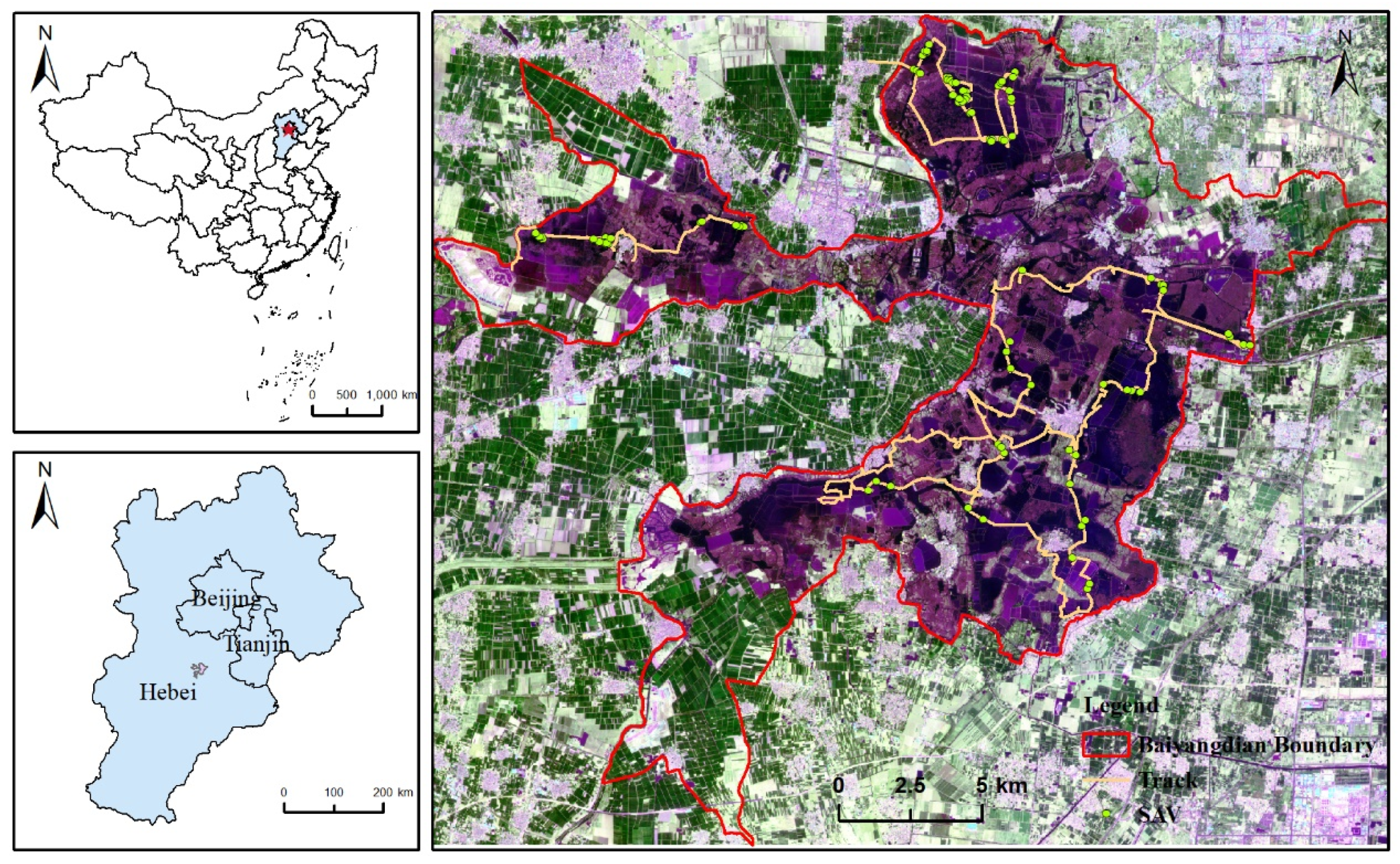
Baiyangdian Lake is located in the middle of the North China Plain, with a geographical location of 115°38′–116°07′E, 38°43′–39°02′N, and a total area of 366 km2. As shown in Figure 1, it is located in Xiong’an New Area, most of which belongs to Anxin County and Xiong County of Hebei Province. It is the largest natural lake on the North China Plain, formed by the confluence of the Yongding River and Hutuo River alluvial fans on the eastern foot of the Taihang Mountains [21]. The lake plays an important role in flood storage, drought prevention, carbon sequestration, biodiversity maintenance, and local climate improvement, so it is known as the “Kidney of North China”. As an important part of Xiong’an New Area, Baiyangdian needs to coordinate the governance of the city, water, forests, fields, and lakes; protect the ecological environment; and restore the function of the “Kidney of North China”. Protecting the ecological environment and restoring the function of the “Kidney of North China” are important steps for the Xiong’an New Area to build a model city of ecological civilization in the new era.
This area has a warm temperate continental monsoon climate, with an average annual temperature of about 12.1 °C. The average annual precipitation is about 563.9 mm, and the precipitation is mainly concentrated in July–August with large interannual changes. The average annual evaporation is about 1369 mm, which is much greater than the amount of precipitation [22]. Baiyangdian Lake consists of 143 lakes of varying sizes that are bounded by dikes and more than 3700 crisscross trenches, forming a complex lake and marsh wetland system [23]. The water depth of most areas in Baiyangdian Lake is between 1 and 4 m. Baiyangdian Lake is rich in animal and plant resources, including fish, crabs, shrimps, and other aquatic species [21]. Common aquatic plants include emergent aquatic vegetation, floating aquatic vegetation, and submerged aquatic vegetation. As shown in Table 1, Baiyangdian aquatic vegetation in this study is divided into three classes for the purpose of analyzing its phenological changes during the year. The first and second classes are floating and emergent aquatic vegetation (FEAV), which are further divided according to whether they have dead branches on the water surface in the spring (see Table 1), and the third class is various types of submerged aquatic vegetation.
2.2. Sentinel-2 Data
The Sentinel-2 constellation consists of two identical satellites operating in sun-synchronous orbits, with a revisit time of five days on the equator and a shorter time toward the poles [24]. Sentinel-2 MSI has 13 spectral bands, including visible light and near-infrared to short-wave infrared spectral bands, with a spatial resolution of 10 m. The Sentinel-2 data provided by the GEE platform were preprocessed (e.g., radiation correction, orthorectification, atmospheric correction). A total of 505 scenes of Sentinel-2 images covering the Baiyangdian area in 2020 were selected from the GEE platform.
2.3. In Situ Survey Data
Field surveys and high-resolution images were used to assess the accuracy of SAV maps. In recent years, our research group has conducted numerous field surveys to the Baiyangdian Lake. The surveys were conducted in May, August, and October of 2020, and each field survey was about 5 days. We cruised through the lakes by boat to obtain the ground truth (see the track in Figure 1). The surveys covered almost all of the SAV growing season and helped to determine the start and end dates of the growing season. To ensure the purity of the sample points, we only recorded pixels with SAV coverage greater than 20%. A handheld GPS instrument was employed to record the geographic location of each aquatic vegetation sampling point, and digital photos above the SAV surface were obtained at each sampling point. The dominant species and growth stages of aquatic vegetation were recorded, and the vegetation coverage of the sampling points was visually estimated within an ~10 × 10 m2 area. Due to a large number of Baiyangdian dikes and fishing nets, some areas were difficult to investigate. The sample points were interpreted through high-resolution images such as those of Google Earth and WorldView-2. Specifically, based on field surveys, areas identified as SAV were analyzed for their characteristics (such as texture and color) on high-resolution images to determine the type of features. Once the features (such as texture and color) of the SAV areas on the high-resolution image were analyzed, they were used to determine the land use type of other unknown areas. A total of 1000 pixel points were generated for accuracy assessment, of which were 250 were SAV sample points and 750 were non-SAV sample points.
3. Methodology
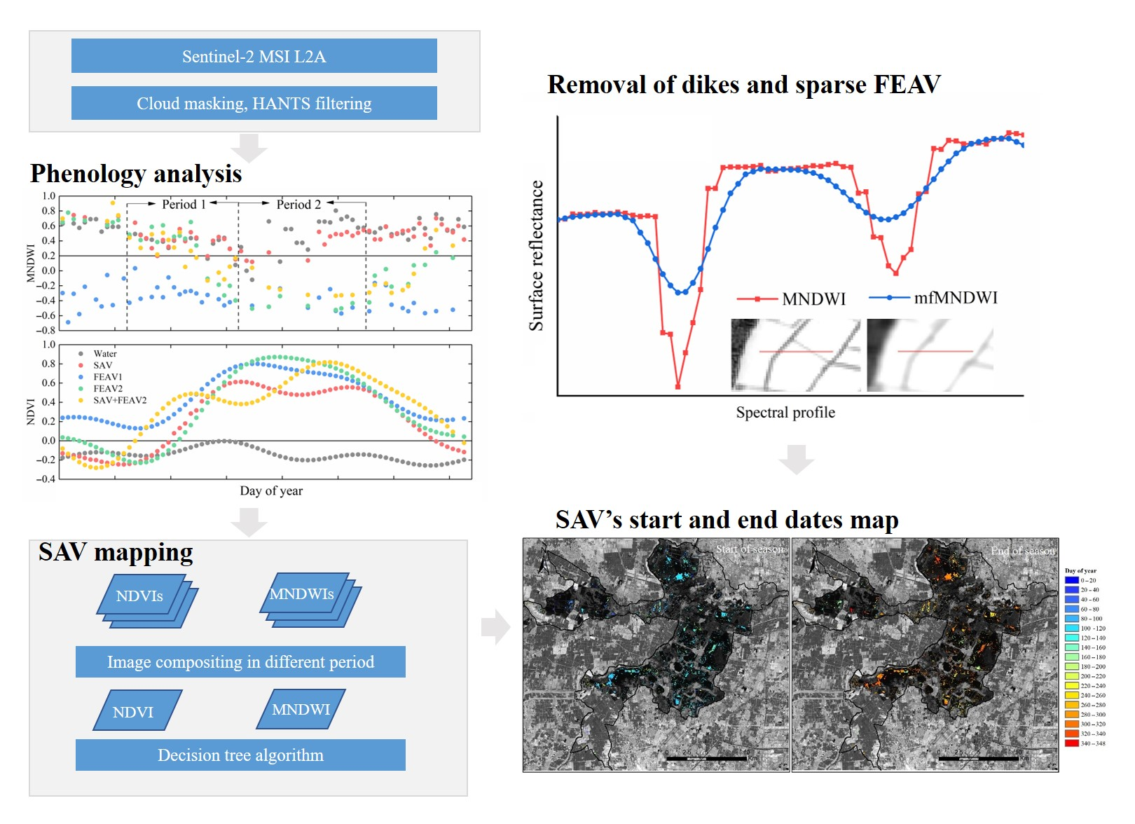
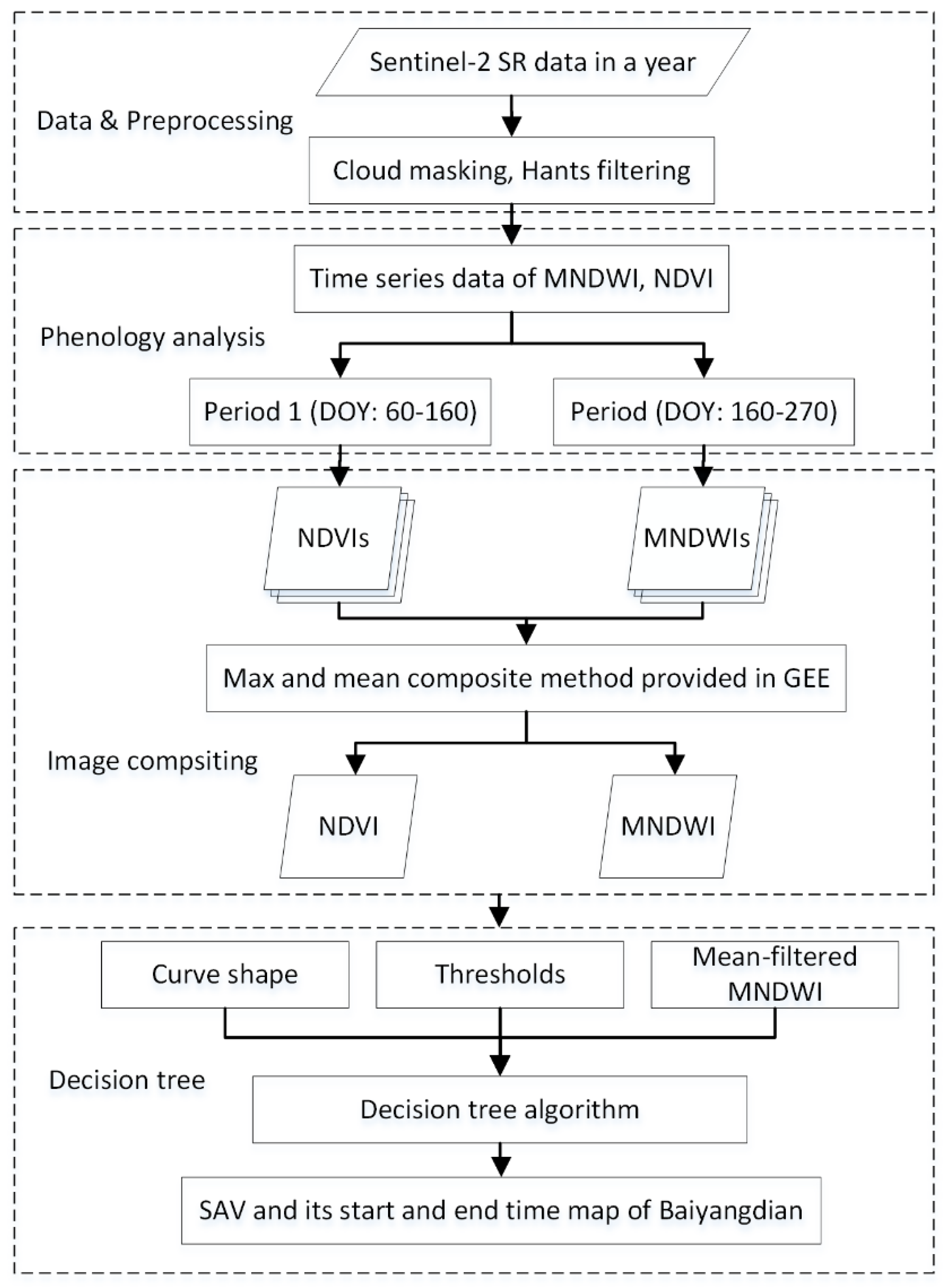
As shown in Figure 2, the method described in this paper mainly includes four parts: Sentinel-2 data preprocessing, phenological analysis of Baiyangdian aquatic vegetation, pixel-based composite of time-series images, and establishment of a decision tree model to determine the distribution and growth of SAV.
3.1. Phenological Characteristics of Aquatic Vegetation in Baiyangdian Lake
3.1.1. Construction of Dense Time-Series NDVI Dataset
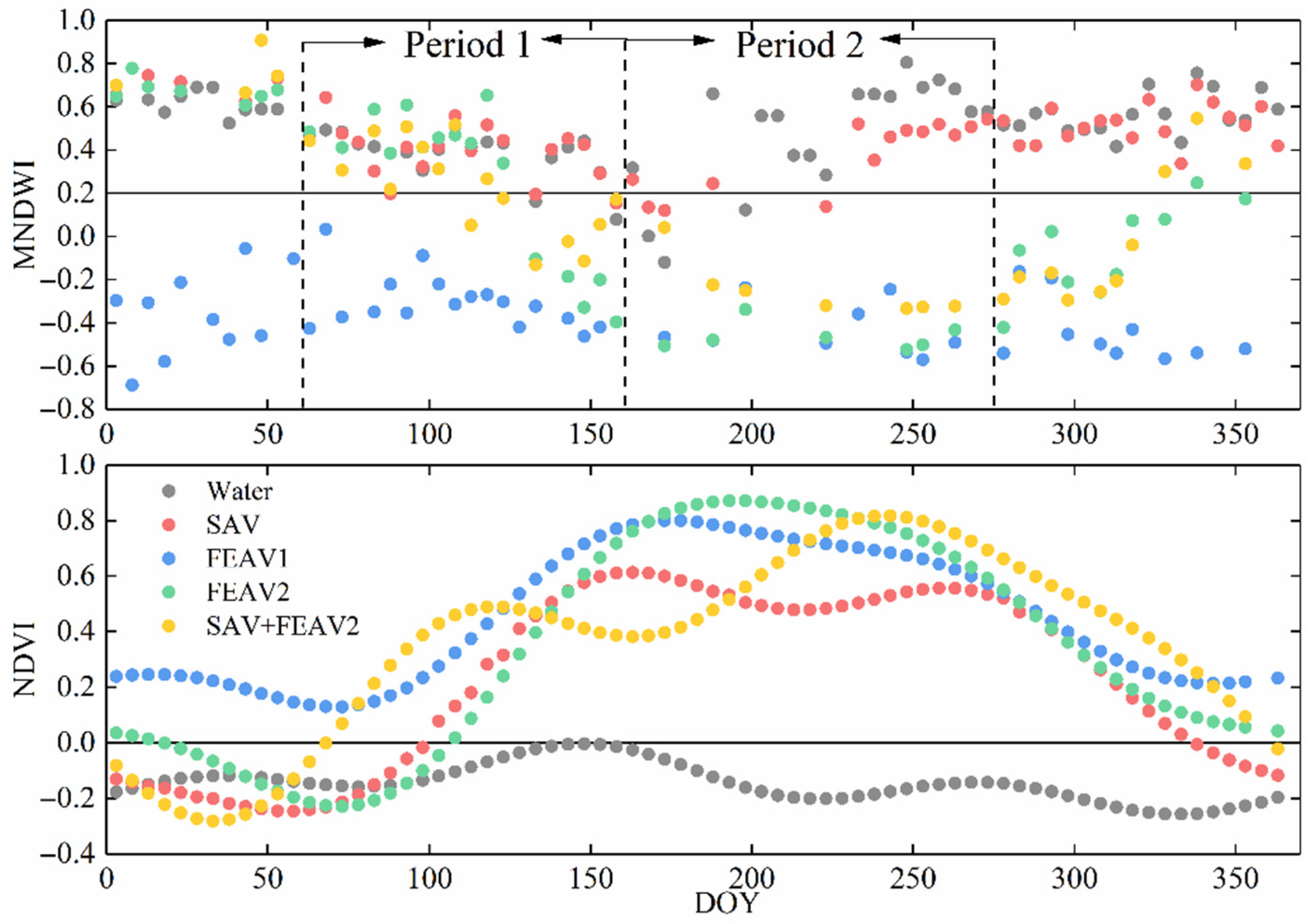
First, we masked the pixels marked as 1 in Bit10 and Bit11 of the QA60 band to remove noise observation pixels such as cirrus clouds and thick clouds to obtain usable pixels for each scene image. The revisit period of Sentinel-2 data in the Baiyangdian Lake area is five days. For areas where images of different orbits overlap, the Sentinel-2 data are median composites used to create a Sentinel-2 image cube with five-day intervals throughout the year. To fill the gaps caused by the excluded low-quality data (clouds, cloud shadows) and eliminate potential noise on the time scale, this study applied harmonic analysis of time series (HANTS) to the annual NDVI time series. The principle of the HANTS algorithm is to remove the abnormal values in the time-series data through the iterative fitting of the least-squares method and realize the decomposition and reconstruction of the curve by the positive and negative transformation of the Fourier transform in the time domain and the frequency domain [25,26]. We obtained the NDVI time-series dataset with a five-day interval (Figure 3) to analyze the phenological changes of different types of aquatic vegetation in Baiyangdian Lake. As the MNDWI index is significantly affected by surface moisture and atmospheric conditions, we did not perform HANTS filtering to obtain this dataset but rather used the original observation data.
3.1.2. Analysis of Key Phenological Characteristics of Aquatic Vegetation
According to the vegetation phenology information obtained from the Baiyangdian field survey, SAV can be roughly divided into two categories. The first category is Potamogeton crispus, and the second category includes Ceratophyllum demersum, Myriophyllum verticillatum, and Potamogeton pectinatus. Type 1 germinated in early March and gradually approached the water surface; it reached its peak in mid-April and became the only dominant species of SAV in the lake; then, it rotted and quickly died out at the end of May. Type 2 generally began to grow in early May with the growing season ending at the end of November.
Based on the measured spectral data of the field survey, this study used the NDVI and the MNDWI to extract SAV. NDVI is closely related to the leaf area index, and it is one of the most extensive indicators for studying vegetation phenology and vegetation biomass changes [27]. MNDWI is often used to extract surface water bodies. Both water bodies and SAV are strongly absorbed in short-wave infrared, so the MNDWI index can be used to identify both water bodies and SAV.
where ρgreen, ρred, ρnir, and ρswir are the surface reflectance values of green, red, near-infrared, and short-wave infrared bands.
As shown in Figure 3, two key phenological characteristics of SAV mapping were determined based on the annual MNDWI curve and the NDVI annual time-series curve filtered by the HANTS method: (1) Through the NDVI time-series curve in Figure 3, it was found that the NDVI value during day of year (doy) 60–160 mainly shows the growth characteristics of Potamogeton crispus. After doy 60, the NDVI value of Potamogeton crispus began to increase rapidly and reached a peak after about 120 days and then began to decay rapidly. As the area may become reoccupied by newly emerging emergent aquatic vegetation (such as lotus), the NDVI curve exhibited another peak around August. The MNDWI index also had obvious characteristics. The MNDWI index of SAV was relatively high in period 1 but dropped rapidly in period 2. (2) The NDVI of type 2 began to increase rapidly around doy 100 and remained relatively stable between doy 160 and 270. Due to the strong absorption of SAV in the short-wave infrared band, its annual MNDWI index had high values.
3.2. A Phenology–Pixel Algorithm for SAV Mapping
3.2.1. Determination of Extraction Threshold
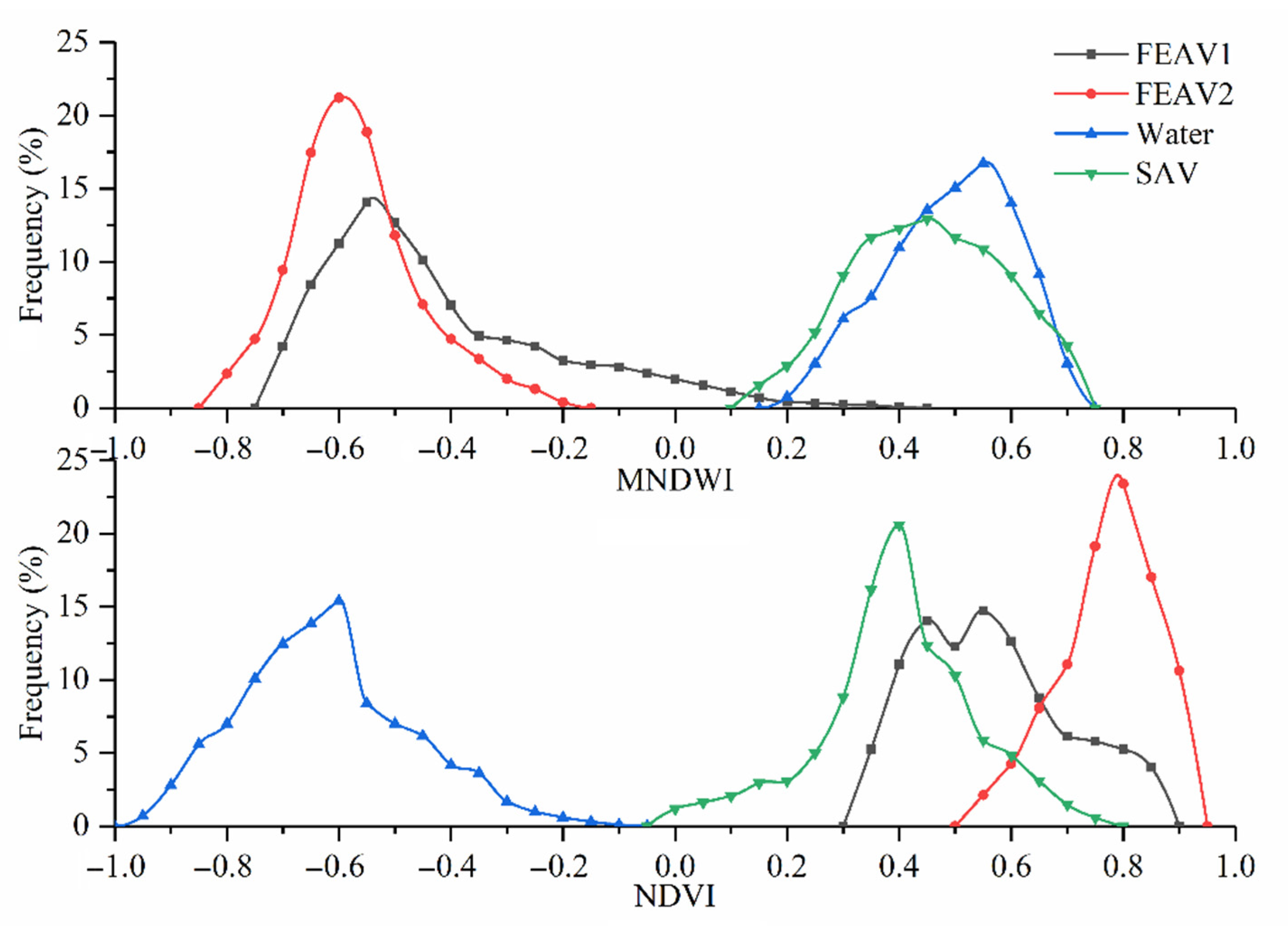
Dai et al. [17] used a single short-wave infrared (SWIR) band threshold to distinguish SAV from FEAV. Due to the influence of atmospheric correction on optical satellite data, the reflectivity of SAV in the short-wave infrared band fluctuates at different times. Therefore, we used the MNDWI index that combines short-wave infrared and green bands to weaken the influence of atmospheric correction. The commonly used vegetation index NDVI was applied to separate SAV and water bodies because SAV still has reflection peaks in the near-infrared and absorption valleys in the red band.
We selected 14,382 data samples from Sentinel-2 images during the vegetation growing season to analyze the separability of aquatic vegetation in Baiyangdian Lake. As shown in Figure 4, about 98.2% of SAV and water bodies had an MNDWI index greater than 0.2, and about 99.3% of SAV had an NDVI index greater than 0. Finally, the extraction index and threshold of SAV were defined as MNDWI > 0.2 and NDVI > 0.
3.2.2. Extraction Steps of Annual SAV Mapping
Step 1: We obtained the mean composite images of MNDWI in each of the two periods, and then we used MNDWI > 0.2 to determine whether the two periods had water bodies and SAV.
Step 2: For pixels where SAV may exist in the previous step, we obtained the maximum composite images of NDVI in each of the two periods, and then we used NDVI > 0 to separate SAV and water bodies.
Step 3: For pixels extracted as SAV in stage 1, it was necessary to add the condition of having a peak in the NDVI curve in stage 1. No additional conditions were required in stage 2.
Step 4: In combining the SAV pixels extracted from the two time periods, the following situations are possible: (1) SAV exists only in period 1, (2) SAV exists only in period 2, and (3) SAV exists in both periods 1 and 2. The three situations were combined to obtain the largest annual spatial distribution range of SAV.
3.2.3. Start and End Time of SAV Growth
Baiyangdian Lake is seriously affected by human activities, and SAV may be destroyed by humans. This study attempted to determine the SAV time of existence by analyzing the changes in NDVI. Equations (3) and (4) show how to determine the Julian day of the start and end of the growing season. If only stage 1 of the pixel is SAV (generally stage 2 is lotus), the time when NDVI is in the trough is defined as the end of the growing season.
where i denotes the day of year (doy), SOS is the start of the season, and EOS is the end of the season.
SOS = NDVIi-5 < 0, NDVIi > 0, NDVIi+5 > 0 ∩ NDVIi-5 < NDVIi < NDVIi+5
EOS = NDVIi-5 > 0, NDVIi > 0, NDVIi+5 < 0 ∩ NDVIi-5 > NDVIi> NDVIi+5
3.2.4. Removal of Dikes and Sparse FEAV
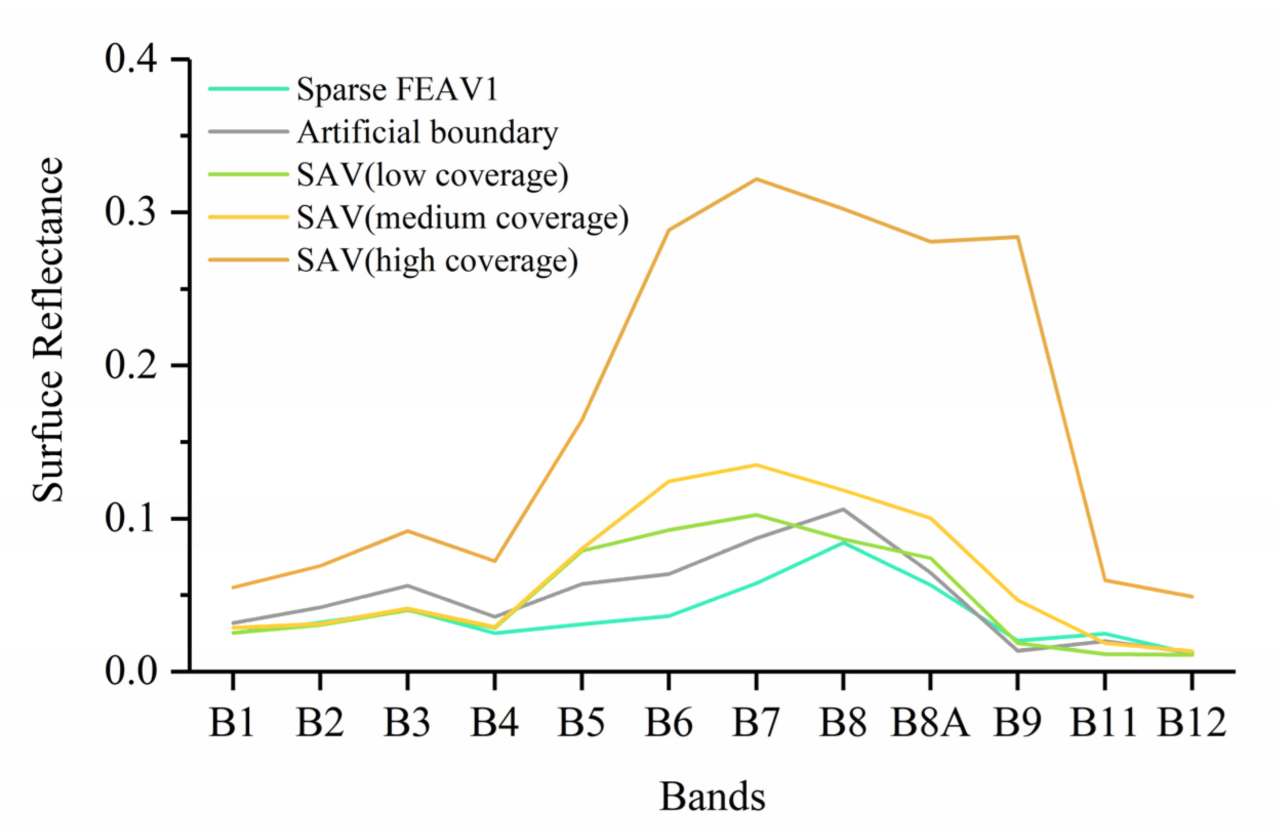
The presence of dikes and sparse FEAV causes misclassification in shallow grass-type lakes. Baiyangdian is artificially divided into grid-like aquaculture areas, and most of the dikes are reeds or woodlands (5–20 m). The spectrum of these mixed pixels is similar to the spectrum of aquatic vegetation (as shown in Figure 5). The coverage of SAVs with low coverage, medium coverage, and high coverage was 20%, 50%, and 80%, respectively. While it is difficult to remove the dikes and sparse FEAV using only the two indicators of NDVI and MNDWI, they have unique textural characteristics that make them easy to distinguish [28].
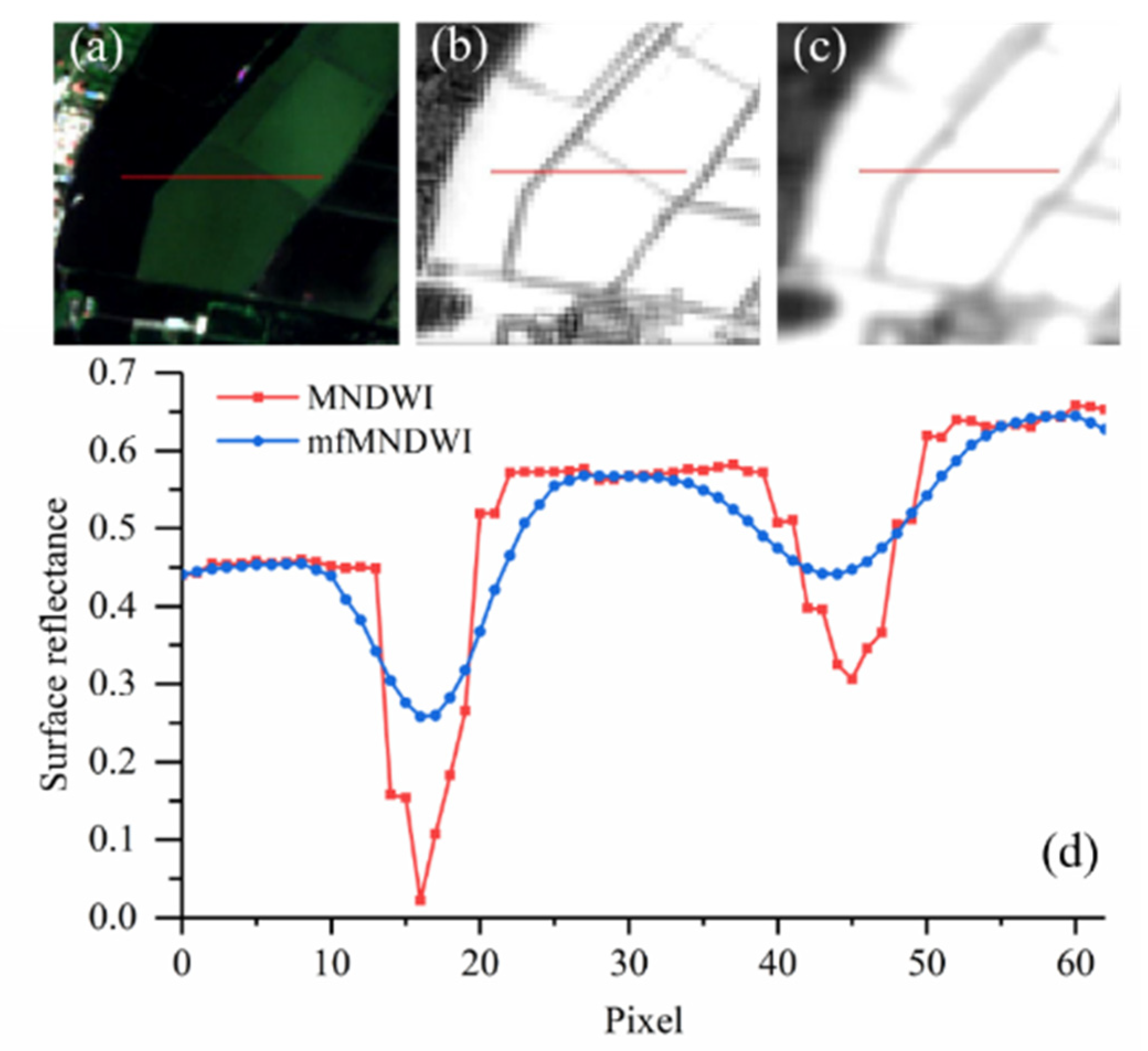
As shown in Figure 6, the mean-filtered MNDWI image (mfMNDWI) was obtained by using 7 × 7 window average filtering on the MNDWI image in the summer. Because the MNDWI pixel value of the water on both sides of the artificial dike is higher than that of the dike, the mean filtering can improve the pixel value of the water mixed pixel in the dike area. Based on this textural feature, we used Equation (5) to determine the mixed pixels containing artificial dikes or sparse reeds.
Boundary = (MNDWI − mfMNDWI) < −0.05
3.3. Accuracy Validation
The stratified random sampling method was used to select sample points. A total of 1000 pixel points were generated based on the obtained SAV map, and the SAV and non-SAV pixels were generated at a ratio of 1:3. We determined whether there was SAV based on Google Earth high-resolution images and nine Sentinel-2 images from March to November. The user’s accuracy, producer’s accuracy, and overall accuracy obtained by the confusion matrix method were used as the evaluation indicators.
4. Results
4.1. Accuracy Assessment of the SAV Map
We evaluated the accuracy of the SAV map of the Baiyangdian Lake in 2020. Approximately 1000 sample points were identified through multiscene images in a year to evaluate the maximum range of annual SAV extracted by this method. As shown in Table 2, the overall accuracy, producer’s accuracy, and user’s accuracy of submerged plants were 94.8%, 87.3%, and 93.3%, respectively. We found that commission errors occur when SAV is sparsely distributed and has a short duration. This is further analyzed in the discussion section.
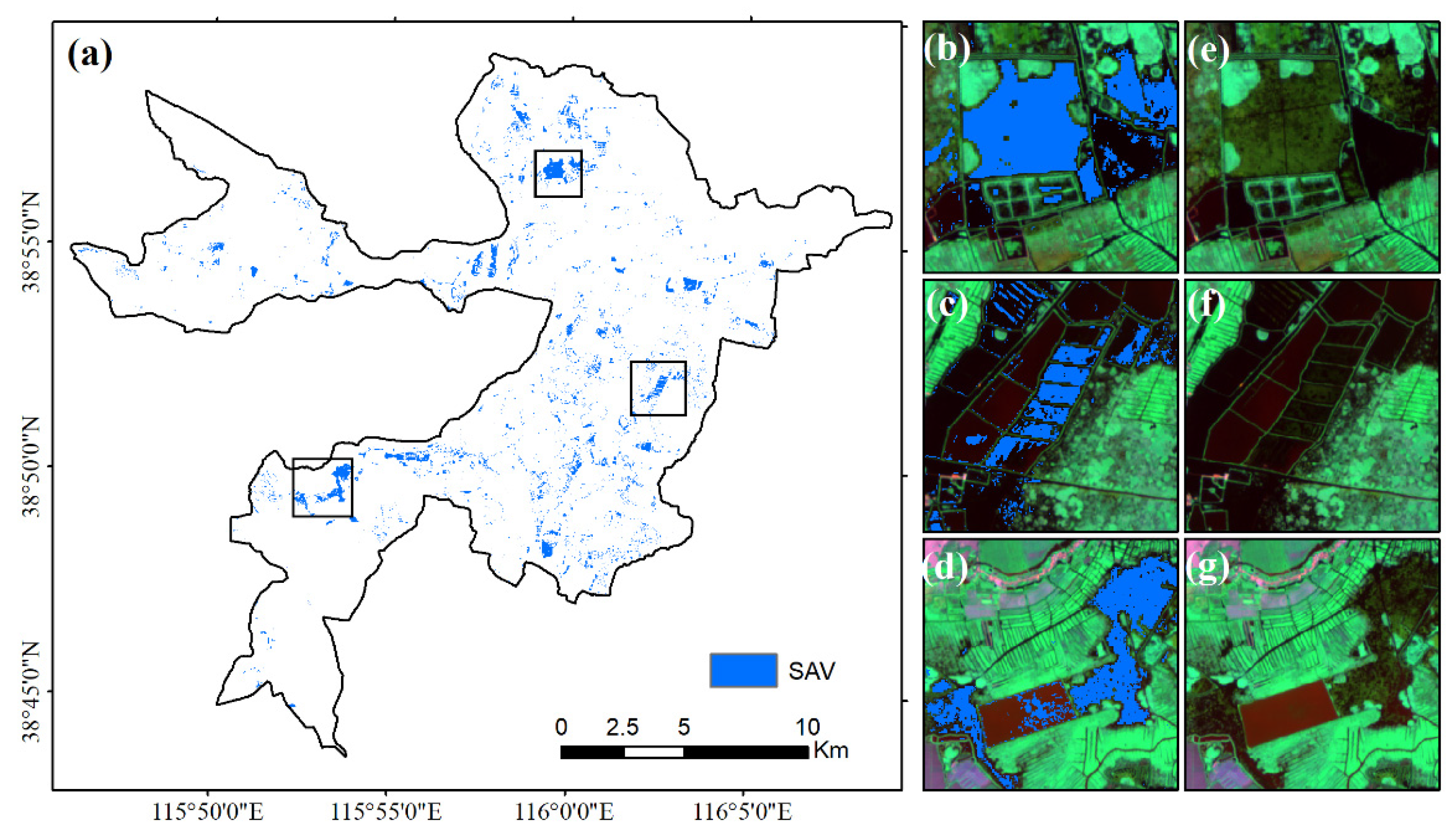
The area of Baiyangdian SAV was about 12.1 km2 in 2020. As shown in Figure 7, most of the dense SAV is distributed in blocks and fills the entire lake and several ponds, such as Shaochedian in the north and Chiyudian in the east. Some SAV appears to be scattered or striped on the edge of the dikes and in relatively open water areas.
4.2. Comparison before and after Removal of Dikes and Sparse FEAV
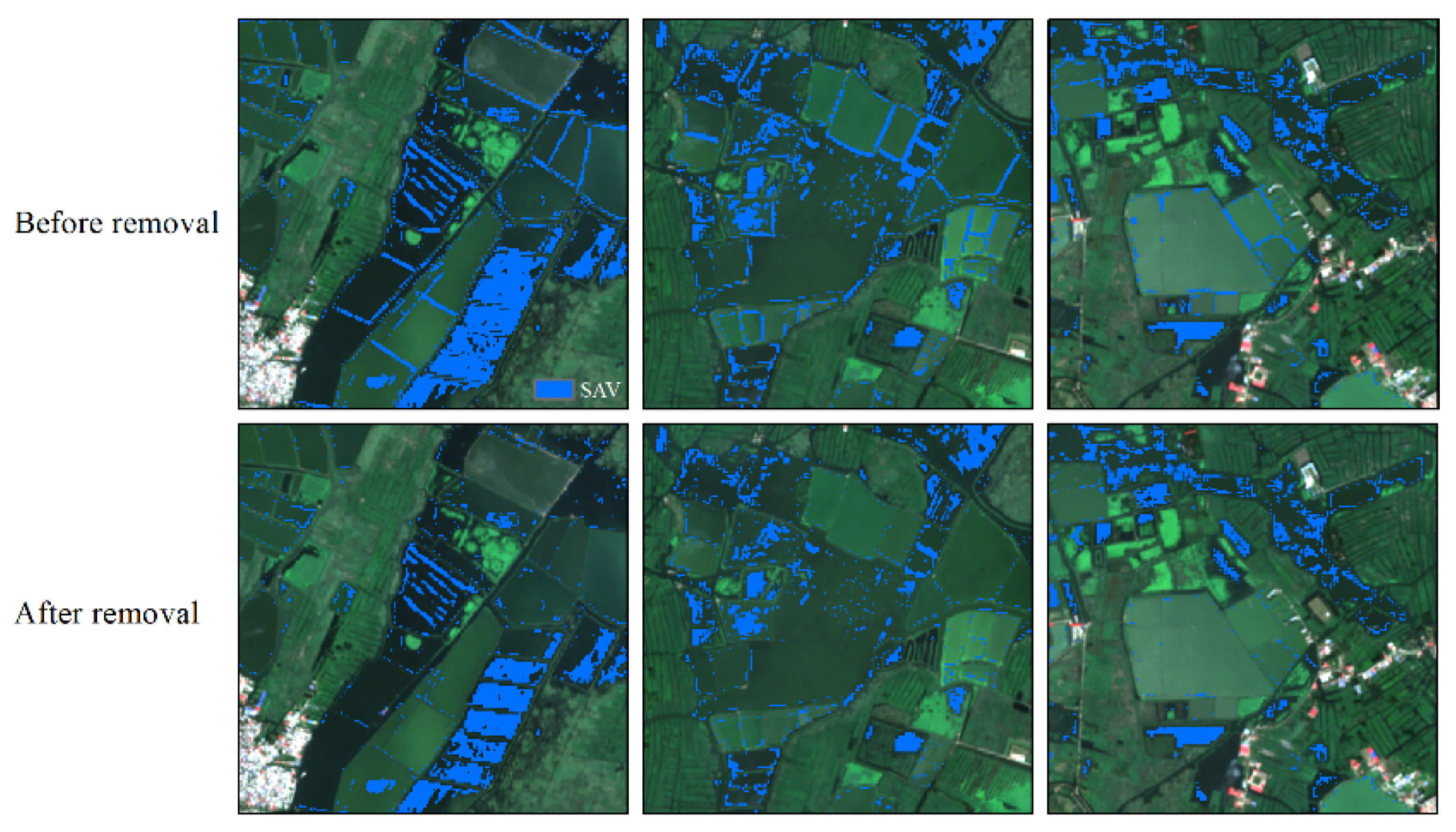
Figure 8 shows the distribution of SAV before and after the removal of dikes and sparse FEAV. SAV was located near the artificial dikes before removal, and the SAV between adjacent ponds was almost connected. The method applied in this study can effectively reduce the commission error with the SAV distribution conforming to reality.
4.3. Growth Time of SAV in Baiyangdian Lake
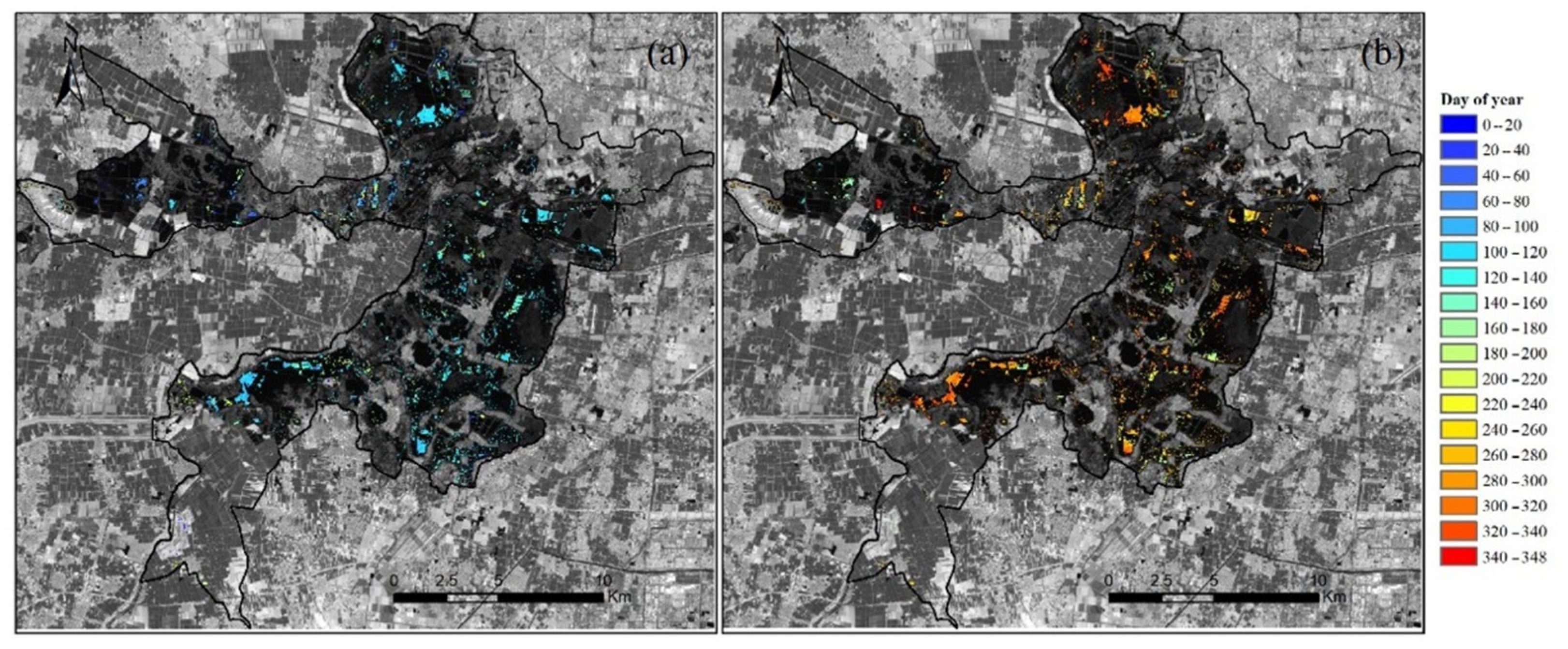
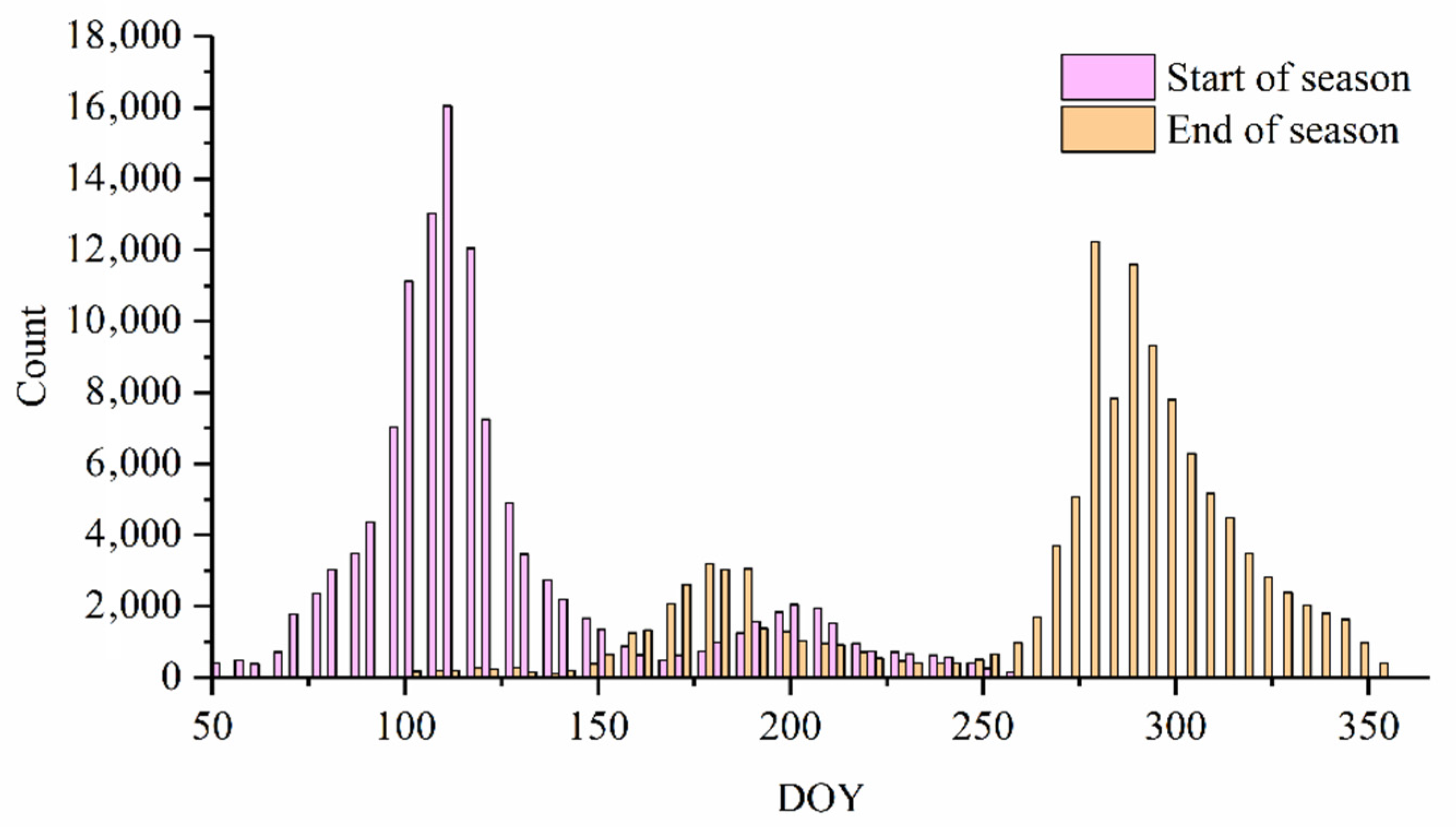
As shown in Figure 9 and Figure 10, we determined the SOS (doy), EOS (doy), and growth duration of SAV. Most SAV grows from spring to the end of autumn. The start time is mostly concentrated within 80–120 days, and the end time is mostly concentrated within 240–320 days. Potamogeton crispus is different from other SAV. It starts to grow around doy 60 and decays from doy 140 to 180. Therefore, SAV is assumed to be Potamogeton crispus when the growth start date is about doy 60. Most Potamogeton crispus is distributed in the Zaozhai Lake in the northwest and the Shaoche Lake area in the north. The bottom of Zaozhai Lake has a higher elevation and a shallower water depth than other areas, which promotes the growth and reproduction of Potamogeton crispus. The ecological water replenishment project in Baiyangdian leads to higher water levels in the spring (the water level is 0.7 m higher in March than in July), which may exacerbate this phenomenon.
5. Discussion
5.1. Advantages of the SAV Mapping Method in This Study
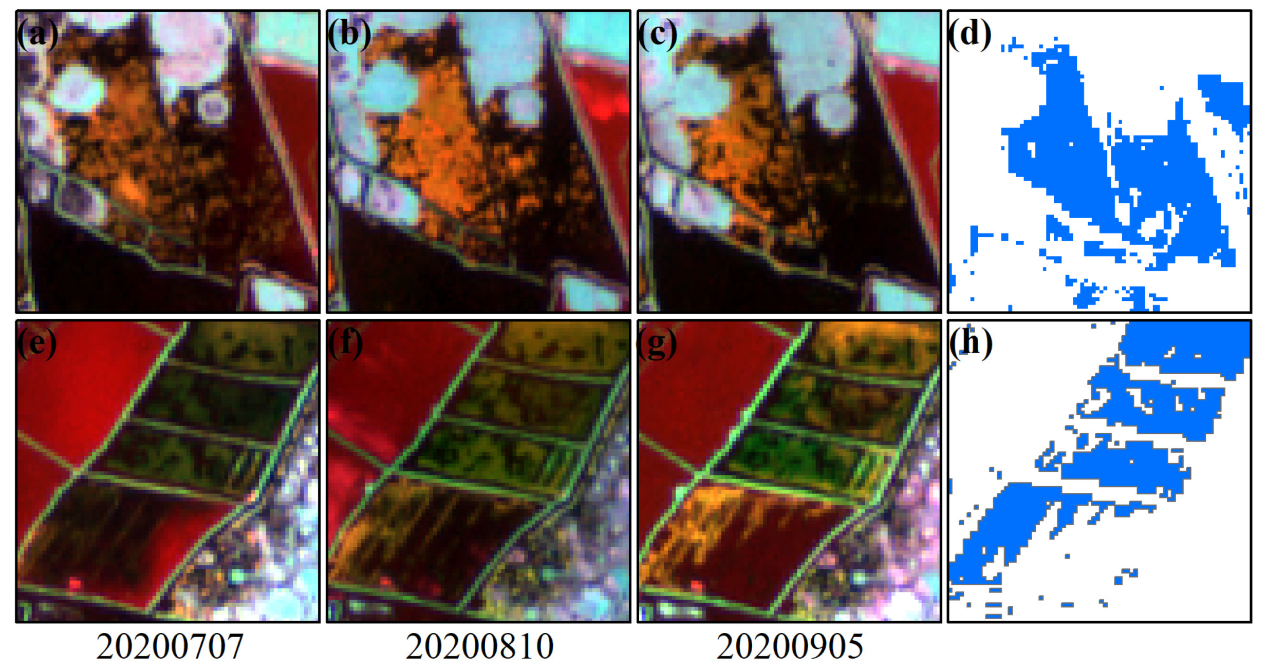
This study proposes a method to monitor SAV by using all available Sentinel-2 images to minimize the uncertainty caused by extracting SAV from a single image. Theoretically, the distribution of SAV is relatively stable due to the vegetation’s strong roots, and the area covered by SAV will not fluctuate significantly during the year. As shown in Figure 11, the distribution of SAV (green is SAV) on the three Sentinel-2 images of July, August, and September is not the same. If only a single image had been used, this information may have been ignored, causing some SAV to be missed.
Luo et al. [15] and Dai et al. [17] both proposed extraction methods based on a series of index and threshold definition methods for a single image. However, they ignored the environmental impact of SAV (such as the depth of the canopy and the growth period) and complicated the calculation of the threshold for each scene image. While their methods work well in open lakes, they have limitations in areas where the underlying surface is broken or complex. Dividing mixed pixels such as sparse FEAV into SAV is easy.
In addition, the method proposed in this study takes into account the phenological characteristics of vegetation. Due to the high mixing of reeds and water bodies during this period, it is possible to observe not only vegetation characteristics in the near-infrared band, but also water characteristics in the short-wave infrared band. In this study, the NDVI curve of Potamogeton crispus had a peak around April, which helped reduce the commission errors caused by reeds growing in the water in spring. Some studies have found that the mixed pixels of FEAV and water bodies are easily misclassified as SAV [29]. In this study, the spatial texture features and phenological characteristics of mixed pixels can be used to reduce misclassification.
The study used the HANTS filtering method to reconstruct the NDVI time series, which can better eliminate abnormal observations and fill in noise observations. Figure 12 compares the curve change before and after filtering of a water pixel. We were able to observe the true-color composite image (R:4, G:3, B:2) of the abnormal fluctuation date of NDVI. It was found that the turbidity of the water body was higher on June 6 and the thin cloud was not recognized by the cloud removal algorithm on June 18. The filtered curve avoids the appearance of these abnormal observations.
5.2. Stable Growth Area of SAV in Baiyangdian Lake
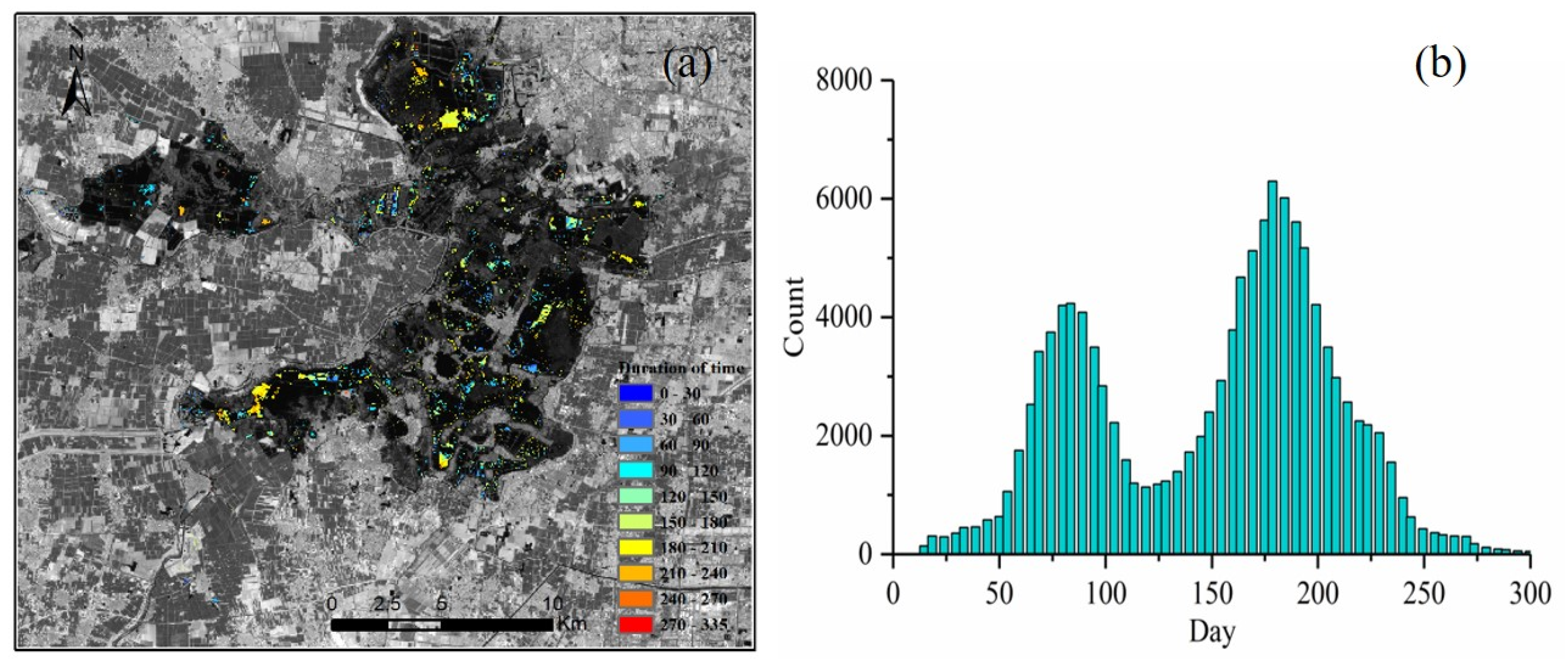
According to the beginning and end time of SAV growth in this study, the duration of SAV growth in Baiyangdian Lake was determined. SAV with a long growth duration is mostly located inside ponds and lakes and is less affected by human activities. As shown in Figure 13, SAV with a growth duration of less than 60 days is basically distributed around Quantou Township and the northeast of Shaoche Lake. Human activities in these areas are significant (such as boat traffic, fishing nets, and engineering activities), making these areas more susceptible to damage by human activities than other areas. In contrast, the growth, coverage, and stability of SAV are relatively high in relatively closed ponds.
Different types of SAV have different growth times. For example, the growth time of Potamogeton crispus in the spring is shorter than that of other types of SAV. The frequency histogram in Figure 13 shows two peaks, with a trough of about 140 days, which is caused by the shorter growth period of Potamogeton crispus.
5.3. Uncertainties and Limitations
Similar to other commonly used SAV extraction algorithms, our method cannot extract SAV in areas with large canopy depths and turbid water bodies throughout the year. Due to the high absorption of water molecules in the near-infrared band, SAV with a large canopy depth cannot be detected [30,31]. The water level in Baiyangdian Lake fluctuates greatly. We tried to compensate for this phenomenon through multitemporal remote sensing images. In addition, the underlying surface of Baiyangdian Lake is more complicated, and some SAV is associated with reed communities and lotus communities. Limited by the image spatial resolution, the method proposed in this study will cause omission errors. At present, there is no suitable method to extract SAV that is covered by lotus leaves. For the problem of mixed pixels, images with higher spatial resolution can be used in the future to minimize the omission error.
In this paper, HANTS harmonic analysis was performed on each pixel to eliminate outliers. Although to a certain extent this analysis can weaken the impact of abnormal observations (bottom mud turning, cloud noise), some SAV that exists for less than 20 days will still be missed.
The NDVI threshold for extracting SAV in this method needs to be slightly modified to apply to other regions. Different from terrestrial remote sensing, the reduced magnitude of the water signal inevitably results in its being disturbed by environmental factors such as atmospheric conditions, water quality, and sun angle in aquatic remote sensing [32,33]. Therefore, the extraction of SAV in different lakes needs to set specific thresholds for local environmental conditions. This study is aimed at the extraction of SAV in grass-type lakes, which may not be applicable to algal-type lakes. The presence of phytoplankton can directly affect the NDVI value in water bodies, which may cause misclassification.
6. Conclusions
Accurately determining the distribution of SAV is of great significance to lake protection planning and water resources management. In this study, based on all available Sentinel-2 images and the phenological and textural characteristics of various aquatic plants, we developed a phenology–pixel method suitable for extracting the spatial distribution and existence time of SAV in a macrophytic lake. The method described in this study effectively eliminated the influence of FEAV and mixed pixels. Accuracy verification showed an overall accuracy of 94.8%, with a user’s accuracy and producer’s accuracy of 93.3% and 87.3%, respectively.
In this study, the peak of NDVI effectively identified Potamogeton crispus and effectively eliminated the influence of low emergent plants in early spring. In addition, according to the textural characteristics of the MNDWI index, the misclassification caused by both sides of the dikes and sparse reeds was eliminated. This method provides an effective way to accurately determine the temporal and spatial distribution of different SAV populations in macrophytic lakes.
Author Contributions
Conceptualization, S.L. and Z.G.; methodology, S.L.; software, S.L.; validation, S.L., Z.G. and Y.W.; formal analysis, J.Z. and W.Z.; investigation, S.L. and Y.W.; writing—original draft preparation, S.L.; writing—review and editing, Z.G.; supervision, Z.G. and W.Z.; project administration, Z.G.; funding acquisition, Z.G. All authors have read and agreed to the published version of the manuscript.
Funding
This research was funded by the National Natural Science Foundation of China (Grant No. 41971381) and the Key Program of Beijing Municipal Bureau of Water (Grant No. TAHP-2018-ZBYY-490S).
Acknowledgments
The authors express their gratitude for the support from the Google Earth Engine platform.
Conflicts of Interest
The authors declare no conflict of interest.
References
- Agostinho, A.A.; Thomaz, S.M.; Gomes, L.C.; Baltar, S.L.S.M. Influence of the macrophyte Eichhornia azurea on fish assemblage of the Upper Paraná River floodplain (Brazil). Aquat. Ecol. 2007, 41, 611–619. [Google Scholar] [CrossRef]
- Barko, J.W.; Gunnison, D.; Carpenter, S.R. Sediment interactions with submersed macrophyte growth and community dynamics. Aquat. Bot. 1991, 41, 41–65. [Google Scholar] [CrossRef]
- Bolpagni, R.; Bresciani, M.; Laini, A.; Pinardi, M.; Matta, E.; Ampe, E.M.; Giardino, C.; Viaroli, P.; Bartoli, M. Remote sensing of phytoplankton-macrophyte coexistence in shallow hypereutrophic fluvial lakes. Hydrobiologia 2014, 737, 67–76. [Google Scholar] [CrossRef]
- Gumbricht, T. Nutrient removal processes in freshwater submersed macrophyte systems. Ecol. Eng. 1993, 2, 1–30. [Google Scholar] [CrossRef]
- Jeppesen, E. The Structuring Role of Submerged Macrophytes in Lakes; Springer: New York, NY, USA, 1998. [Google Scholar]
- Orth, R.J.; Carruthers, T.J.B.; Dennison, W.C.; Duarte, C.M.; Fourqurean, J.W.; Heck, K.L.; Hughes, A.R.; Kendrick, G.A.; Kenworthy, W.J.; Olyarnik, S. A Global Crisis for Seagrass Ecosystems. BioScience 2006, 56, 987–996. [Google Scholar] [CrossRef] [Green Version]
- Zhang, Y.; Liu, X.; Qin, B.; Shi, K.; Deng, J.; Zhou, Y. Aquatic vegetation in response to increased eutrophication and degraded light climate in Eastern Lake Taihu: Implications for lake ecological restoration. Sci. Rep. 2016, 6, 23867. [Google Scholar] [CrossRef] [PubMed]
- Folke, C.; Carpenter, S.; Walker, B.; Scheffer, M.; Elmqvist, T.; Gunderson, L.; Holling, C.S. Regime Shifts, Resilience, and Biodiversity in Ecosystem Management. Annu. Rev. Ecol. Evol. Syst. 2004, 35, 557–581. [Google Scholar] [CrossRef] [Green Version]
- Luo, J.; Li, X.; Ma, R.; Li, F.; Duan, H.; Hu, W.; Qin, B.; Huang, W. Applying remote sensing techniques to monitoring seasonal and interannual changes of aquatic vegetation in Taihu Lake, China. Ecol. Indic. 2016, 60, 503–513. [Google Scholar] [CrossRef]
- Espel, D.; Courty, S.; Auda, Y.; Sheeren, D.; Elger, A. Submerged macrophyte assessment in rivers: An automatic mapping method using Pléiades imagery. Water Res. 2020, 186, 116353. [Google Scholar] [CrossRef]
- Luo, J.; Duan, H.; Ma, R.; Jin, X.; Huang, W. Mapping species of submerged aquatic vegetation with multi-seasonal satellite images and considering life history information. Int. J. Appl. Earth Obs. Geoinf. 2017, 57, 154–165. [Google Scholar] [CrossRef] [Green Version]
- Wang, S.; Gao, Y.; Li, Q.; Gao, J.; Zhai, S.; Zhou, Y.; Cheng, Y. Long-term and inter-monthly dynamics of aquatic vegetation and its relation with environmental factors in Taihu Lake, China. Sci. Total Environ. 2018, 651, 367–380. [Google Scholar] [CrossRef] [PubMed]
- Villa, P.; Mousivand, A.; Bresciani, M. Aquatic vegetation indices assessment through radiative transfer modeling and linear mixture simulation. Int. J. Appl. Earth Obs. Geoinf. 2014, 30, 113–127. [Google Scholar] [CrossRef]
- Zhao, D.; Lv, M.; Jiang, H.; Cai, Y.; Xu, D. Spatio-Temporal Variability of Aquatic Vegetation in Taihu Lake over the Past 30 Years. PLoS ONE 2013, 8, e66365. [Google Scholar] [CrossRef] [Green Version]
- Luo, J.; Ma, R.; Duan, H.; Hu, W.; Zhu, J.; Huang, W.; Lin, C. A New Method for Modifying Thresholds in the Classification of Tree Models for Mapping Aquatic Vegetation in Taihu Lake with Satellite Images. Remote Sens. 2014, 6, 7442–7462. [Google Scholar] [CrossRef] [Green Version]
- Brooks, C.; Grimm, A.; Shuchman, R.; Sayers, M.; Jessee, N. A satellite-based multi-temporal assessment of the extent of nuisance Cladophora and related submerged aquatic vegetation for the Laurentian Great Lakes. Remote Sens. Environ. 2015, 157, 58–71. [Google Scholar] [CrossRef]
- Dai, Y.; Feng, L.; Hou, X.; Tang, J. An automatic classification algorithm for submerged aquatic vegetation in shallow lakes using Landsat imagery. Remote Sens. Environ. 2021, 260, 112459. [Google Scholar] [CrossRef]
- Gong, Z.; Liang, S.; Wang, X.; Pu, R. Remote Sensing Monitoring of the Bottom Topography in a Shallow Reservoir and the Spatiotemporal Changes of Submerged Aquatic Vegetation Under Water Depth Fluctuations. IEEE J. Sel. Top. Appl. Earth Obs. Remote Sens. 2021, 14, 5684–5693. [Google Scholar] [CrossRef]
- Zhu, J.; Zhou, Y.; Wang, S.; Wang, L.; Liu, W.; Li, H.; Mei, J. Analysis of changes of Baiyangdian wetland from 1975 to 2018 based on remote sensing. J. Remote Sens. 2019, 23, 971–986. [Google Scholar]
- Liu, J.; Feng, Q.; Gong, J.; Zhou, J.; Liang, J.; Li, Y. Winter wheat mapping using a random forest classifier combined with multi-temporal and multi-sensor data. Int. J. Digit. Earth 2018, 11, 783–802. [Google Scholar] [CrossRef]
- Junhong, B.; Jingsi, F.; Laibin, H.; Wei, D.; Ainong, L.; Bo, K. Landscape pattern evolution and its driving factors of Baiyangdian lake-marsh wetland system. Geogr. Res. 2013, 32, 1634–1644. [Google Scholar]
- Zhang, M.; Gong, Z.; Zhao, W.; Duo, A. Landscape pattern change and the driving forces in Baiyangdian wetland from 1984 to 2014. Acta Ecol. Sin. 2016, 36, 4780–4791. [Google Scholar]
- Wang, K.; Li, H.; Wu, A.; Li, M.; Zhou, Y.; Li, W.P. An Analysis of the Evolution of Baiyangdian Wetlands in Hebei Province with Artificial Recharge. Acta Geosci. Sin. 2018, 39, 549–558. [Google Scholar]
- Drusch, M.; Del Bello, U.; Carlier, S.; Colin, O.; Fernandez, V.; Gascon, F.; Hoersch, B.; Isola, C.; Laberinti, P.; Martimort, P.; et al. Sentinel-2: ESA’s Optical High-Resolution Mission for GMES Operational Services. Remote Sens. Environ. 2012, 120, 25–36. [Google Scholar] [CrossRef]
- Lin, Z.; Xingguo, M. Phenologies from harmonics analysis of AVHRR NDVI time series. Trans. CSAE 2006, 12, 138–144. [Google Scholar]
- Li, J.; Liu, H.B.; Li, C.; Li, L. Changes of Green-up Day of Vegetation Growing Season Based on GIMMS 3g NDVI in Northern China in Recent 30 Years. Sci. Geogr. Sin. 2017, 37, 620–629. [Google Scholar]
- Xiao, X.; Biradar, C.; Czarnecki, C.; Alabi, T.; Keller, M. A Simple Algorithm for Large-Scale Mapping of Evergreen Forests in Tropical America, Africa and Asia. Remote Sens. 2009, 1, 355–374. [Google Scholar] [CrossRef] [Green Version]
- Meng, Y.; Du, P.; Wang, X.; Bai, X.; Guo, S. Monitoring Human-induced Surface Water Disturbance around Taihu Lake since 1984 by Time Series Landsat Images. IEEE J. Sel. Top. Appl. Earth Obs. Remote Sens. 2020, 13, 3780–3789. [Google Scholar] [CrossRef]
- Chen, Q.; Yu, R.; Hao, Y.; Wu, L.; Zhang, W.; Zhang, Q.; Bu, X. A New Method for Mapping Aquatic Vegetation Especially Underwater Vegetation in Lake Ulansuhai Using GF-1 Satellite Data. Remote Sens. 2018, 10, 1279. [Google Scholar] [CrossRef] [Green Version]
- Vahtme, E.; Kutser, T.; Paavel, B. Performance and Applicability of Water Column Correction Models in Optically Complex Coastal Waters. Remote Sens. 2020, 12, 1861. [Google Scholar] [CrossRef]
- Zhou, G.; Yang, S.; Sathyendranath, S.; Platt, T. Canopy modeling of aquatic vegetation: A geometric optical approach (AVGO). Remote Sens. Environ. 2020, 245, 111829. [Google Scholar] [CrossRef]
- Bustamante, J.; Pacios, F.; Diaz-Delgado, R.; Aragones, D. Predictive models of turbidity and water depth in the Doana marshes using Landsat TM and ETM+ images. J. Environ. Manag. 2009, 90, 2219–2225. [Google Scholar] [CrossRef] [PubMed]
- Silva, T.; Costa, M.; Melack, J.M.; Novo, E. Remote sensing of aquatic vegetation: Theory and applications. Environ. Monit. Assess. 2008, 140, 131–145. [Google Scholar] [CrossRef] [PubMed]
Figure 1.
Location of Baiyangdian Lake.

Figure 2.
Flowchart of pixel- and phenology-based SAV mapping based on Sentinel-2 data.

Figure 3.
The seasonal dynamics of MNDWI and NDVI indices of various aquatic vegetation types in Baiyangdian Lake.
Figure 3.
The seasonal dynamics of MNDWI and NDVI indices of various aquatic vegetation types in Baiyangdian Lake.

Figure 4.
Spectral characteristics of FEAV1, FEAV2, SAV, and water sampling points.

Figure 5.
Spectral characteristics of sparse FEAV, artificial dikes, and SAV on the Sentinel-2 image.
Figure 5.
Spectral characteristics of sparse FEAV, artificial dikes, and SAV on the Sentinel-2 image.

Figure 6.
Mean filtering of MNDWI: (a) the original true-color image; (b) the single band of the MNDWI image; (c) the single band of the mfMNDWI image; and (d) the profile of the MNDWI and mfMNDWI image.
Figure 6.
Mean filtering of MNDWI: (a) the original true-color image; (b) the single band of the MNDWI image; (c) the single band of the mfMNDWI image; and (d) the profile of the MNDWI and mfMNDWI image.

Figure 7.
Maximum distribution of SAV in Baiyangdian Lake in 2020: (a–d) classified maps: (e–g) the original image (band combination R: B4, G: B8, B: B11).
Figure 7.
Maximum distribution of SAV in Baiyangdian Lake in 2020: (a–d) classified maps: (e–g) the original image (band combination R: B4, G: B8, B: B11).

Figure 8.
Removal of dikes and sparse FEAV in Baiyangdian Lake.

Figure 9.
The start and end of SAV growth in Baiyangdian in 2020: (a) start time of SAV growth; (b) end time of SAV growth.
Figure 9.
The start and end of SAV growth in Baiyangdian in 2020: (a) start time of SAV growth; (b) end time of SAV growth.

Figure 10.
Frequency histogram of SAV growth in Baiyangdian Lake in 2020.

Figure 11.
Changes in SAV on Sentinel-2 images at different times: (a–c,e–g) original image (band combination R: B4, G: B8, B: B11); (d,h) SAV map extracted in this study.
Figure 11.
Changes in SAV on Sentinel-2 images at different times: (a–c,e–g) original image (band combination R: B4, G: B8, B: B11); (d,h) SAV map extracted in this study.

Figure 12.
Comparison of NDVI pixel values of a water pixel before and after HANTS filtering ((a–d) are true-color display images).
Figure 12.
Comparison of NDVI pixel values of a water pixel before and after HANTS filtering ((a–d) are true-color display images).

Figure 13.
Growth duration of SAV in Baiyangdian Lake in 2020: (a) the spatial distribution of the growth duration of SAV; (b) the frequency histogram of growth duration.
Figure 13.
Growth duration of SAV in Baiyangdian Lake in 2020: (a) the spatial distribution of the growth duration of SAV; (b) the frequency histogram of growth duration.


Table 1.
Categories of aquatic vegetation in Baiyangdian Lake.
| Class | Type | Dominant Species |
|---|---|---|
| FEAV (floating-leaved and emergent aquatic vegetation) | FEAV1 | Phragmites communis, Typha angustifolia |
| FEAV2 | Nelumbo nucifera, Lemna minor, Salvinia natans | |
| SAV (submerged aquatic vegetation) | SAV | Potamogeton crispus, Ceratophyllum demersum, Myriophyllum verticillatum, Potamogeton pectinatus |
Table 2.
Classification accuracy of SAV map of Baiyangdian Lake in 2020.
| Class | PA (%) | UA (%) | OA (%) |
|---|---|---|---|
| SAV | 87.3 | 93.3 | 94.8 |
| Non-SAV | 97.6 | 95.3 |
Publisher’s Note: MDPI stays neutral with regard to jurisdictional claims in published maps and institutional affiliations. |
© 2022 by the authors. Licensee MDPI, Basel, Switzerland. This article is an open access article distributed under the terms and conditions of the Creative Commons Attribution (CC BY) license (https://creativecommons.org/licenses/by/4.0/).
Share and Cite
MDPI and ACS Style
Liang, S.; Gong, Z.; Wang, Y.; Zhao, J.; Zhao, W. Accurate Monitoring of Submerged Aquatic Vegetation in a Macrophytic Lake Using Time-Series Sentinel-2 Images. Remote Sens. 2022, 14, 640. https://doi.org/10.3390/rs14030640
AMA Style
Liang S, Gong Z, Wang Y, Zhao J, Zhao W. Accurate Monitoring of Submerged Aquatic Vegetation in a Macrophytic Lake Using Time-Series Sentinel-2 Images. Remote Sensing. 2022; 14(3):640. https://doi.org/10.3390/rs14030640
Chicago/Turabian StyleLiang, Shuang, Zhaoning Gong, Yingcong Wang, Jiafu Zhao, and Wenji Zhao. 2022. "Accurate Monitoring of Submerged Aquatic Vegetation in a Macrophytic Lake Using Time-Series Sentinel-2 Images" Remote Sensing 14, no. 3: 640. https://doi.org/10.3390/rs14030640
Note that from the first issue of 2016, this journal uses article numbers instead of page numbers. See further details here.