
A Semi-Empirical Anisotropy Correction Model for UAS-Based Multispectral Images of Bare Soil


1
Georges Lemaître Centre for Earth and Climate Research, Earth and Life Institute, Université catholique de Louvain, 1348 Louvain-La-Neuve, Belgium
2
Remote Sensing Unit, Vlaams Instituut voor Technologisch Onderzoek (VITO), Boeretang 200, 2400 Mol, Belgium
3
FNRS Belgium, Rue d’Egmont 5, 1000 Bruxelles, Belgium
*
Author to whom correspondence should be addressed.
Remote Sens. 2022, 14(3), 537; https://doi.org/10.3390/rs14030537
Submission received: 29 December 2021
/
Revised: 17 January 2022
/
Accepted: 21 January 2022
/
Published: 23 January 2022
(This article belongs to the Special Issue Innovative Belgian Earth Observation Research for the Environment)
Abstract
:The recent developments in the performance and miniaturization of uncrewed aircraft systems (UAS) and multispectral imaging sensors provide new tools for the assessment of the spatial and temporal variability of soil properties at sub-meter resolution and at relatively low costs, in comparison to traditional chemical analysis. The accuracy of multispectral data is nevertheless influenced by the anisotropic behaviour of natural surfaces, framed in the general theory of the bidirectional reflectance distribution function (BRDF). Accounting for BRDF effects in multispectral data is paramount before formulating any scientific interpretation. This study presents a semi-empirical spectral normalization methodology for UAS-based multispectral imaging datasets of bare soils to account for the effects of the BRDF, based on the application of an anisotropy factor (ANIF). A dataset of images from 15 flights over bare soil fields in the Belgian loam belt was used to calibrate a model relating the ANIF to a wide range of illumination geometry conditions by using only two angles: relative sensor-pixel-sun zenith and relative sensor-pixel-sun azimuth. The employment of ANIF-corrected images for multispectral orthomosaic generation with photogrammetric software provided spectral maps free of anisotropic-related artefacts in most cases, as assessed by several ad hoc indexes, and was also tested on an independent validation set. Most notably, the standard deviation in the measured reflectance of the same georeferenced point by different pictures decreased from 0.032 to 0.023 (p < 0.05) in the calibration dataset and from 0.037 to 0.030 in the validation dataset. The validation dataset, however, showed the presence of some systematic errors, the causes of which require further investigation.
1. Introduction
Diffuse reflectance soil spectroscopy provides a good alternative that may be used to enhance or replace conventional methods of soil analysis, as it is rapid, timely, less expensive, non-destructive, and allows for the simultaneous characterization of various soil properties [1]. Soil spectroscopy is currently a mature discipline thanks to continuous improvements since the mid-1960s [2]. The recent developments in uncrewed aircraft systems (UAS) [3] and technological advancements in the performance and miniaturization of lightweight spectrophotometers [4] provide a toolset for the flexible assessment of the spatial and temporal variability of soil properties at a high resolution (<1 m). Hyper and multispectral imaging sensors, in particular, have been successfully employed for the UAS-based remote sensing of several soil properties in several studies [5,6,7]. The accuracy of spectral remote sensing, however, is challenged by environmental conditions (illumination and atmospheric interactions), measurement protocols, data-processing procedures, and specific sensor characteristics. It is thus critical to understand both the potential and the limitations of this technology before using its data products to study earth system processes [8].
One of the biggest challenges for spectral sensing is that the reflectance of natural surfaces shows anisotropic behaviour, i.e., measured reflectance varies with illumination and viewing geometry. This results in spectral variability not only from different angular measurements and times of the day, but also within the field of view of single images. The theoretical framework for modelling the angular effects occurring between the illumination source, sensor and measured surface has been formulated as the bidirectional reflectance distribution function (BRDF) [9]. Several physical, empirical or semi-empirical models have been developed in an attempt to normalize spectral data with the parametrization of the BRDF [10]. Traditionally, BRDF model calibrations were obtained by performing multi-angular reflectance measurements using complex goniometer setups, but currently, aerial digital imaging provides an alternative platform to field goniometer systems for performing multi-angular reflectance measurements [11]. The advantage in the employment of imaging setups lies in the fact that the field of view of each image can provide a range of measurement geometries and, thus, spectral interactions between the illumination source and the measured surface [12]. In this regard, several empirical methods were developed to use the statistics of images taken on flat homogeneous surfaces to normalize off-nadir reflectance values with those obtained at nadir, with the use of an anisotropy factor (ANIF) [13,14].
Addressing BRDF-related issues in data from remote sensing and imaging spectroscopy is of primary importance to ensure their accuracy before attempting any further analysis. For a few years, UAS multispectral data have been used to infer the spatial variability of soil properties at very high spatial resolution. However, to the best of our knowledge, a thorough understanding of the bias introduced by using uncorrected image datasets is still very limited and a generally applicable workflow to construct and apply bare soil BRDF models is not available. A preliminary analysis from our own bare soil multispectral datasets that were not corrected showed that the resulting orthomosaics exhibited prominent spectral aberrances in the form of “stripes” of different reflectance intensities, which were parallel and coincided with the drone flight lines. The full potential of multispectral imaging for bare soil applications has therefore not been fully reached.
The primary objective of this article is to elaborate a semi-empirical correction methodology for multispectral imaging datasets to account for the effects of the BRDF, based on the calculation of an anisotropy factor (ANIF) calibrated from UAS-based hemispherical-directional [6,14] bare soil reflectance measurements. A secondary objective is to evaluate the beneficial effects of this correction method on the quality of structure from motion (SfM)-based multispectral orthomosaics, using an elaborated UAS data collection campaign of 15 flights conducted in the Belgian loam belt.
To accomplish this, sensor position and orientation data obtained from GPS measurements and SfM-based bundle adjustment algorithms were used to relate observation and illumination angles to soil anisotropy effects at the image level. The resulting data were then used to test different modelling approaches and to provide a consistent image correction workflow. Finally, the orthomosaic products obtained with commercial SfM software using original and corrected images were analytically compared for an analysis of the reduction/elimination of the “striping” artefact and the stability of the spectral measurement when explicitly considering BRDF effects in bare soils.
2. Materials and Methods
2.1. Multispectral Imaging System
The multispectral imaging system used to collect data was a MicaSense RedEdge-M (Micasense Inc., Seattle, WA, USA). This widely used system consists of an array of five synchronized cameras, each with a distinct narrowband filter providing spectral bands centred at 475, 560, 668, 717 and 840 nm wavelengths, with a bandwidth (full width at half maximum) of 20, 20, 10, 40 and 10 nm, respectively. The image resolution is 1280 × 960 pixels with a 3.75 µm pixel pitch, and the camera features a focal length of 5.4 mm, resulting in a 47.2° cross-track field of view (FOV) and a 36.2° along-track FOV. A diffuse irradiance sensor array with similar spectral band characteristics (the so-called downwelling light sensor, or DLS) is mounted on top of the drone in the same optical axis as the camera array and is wired to the main unit to provide synchronized irradiance data. The DLS unit also includes an on-board standalone L1 GPS and inertial measurement unit (IMU) to provide location and orientation measurements (positioning accuracy of 2–5/10 m in xy/z and orientation accuracy of 2–5/5–15° in roll, pitch/yaw). The multispectral imaging system stores a set of five TIFF image files (corresponding to the spectral bands) for every image acquisition point, for which their respective irradiance level and a common GPS position and IMU orientation are saved in the image EXIF and XMP metadata. A calibrated reflectance panel (CRP) of ca. 50% grey reflectance provided by the camera manufacturer was used to convert raw image radiance values to reflectance.
2.2. Data Collection and Pre-Processing
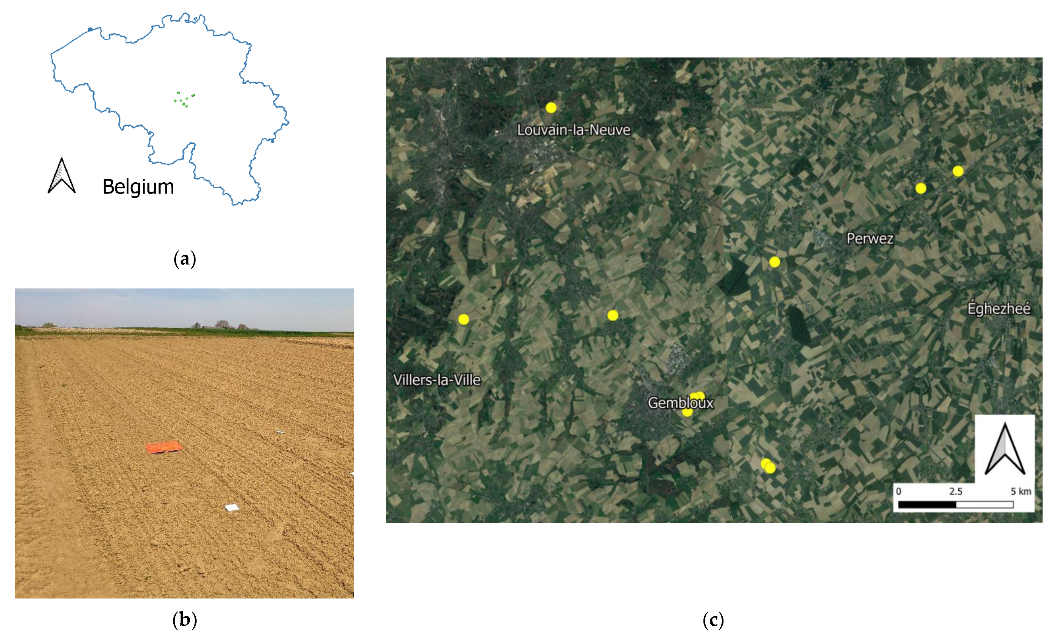
A series of UAS flights with the Rededge-M rigidly mounted on a custom-made quadcopter drone was conducted over bare soil fields in the Belgian loam belt between 2018 and 2021 (flight information is summarized in Table 1, locations are shown in Figure 1a,c). The flights were conducted under clear sky conditions, on dry soil. The fields were in seedbed conditions, with very low roughness (example provided in Figure 1b), very low stoniness, no growing vegetation and very limited vegetation residue. Soils in the area are classified as silt-loam by texture according to the USDA classification. Flight altitude was ca. 45 m above ground level, resulting in ca. 3 cm ground sample distance (GSD). Flight speed was set to 5–6 m/s to ensure a frontal image overlap of 80%, while interline distance was set to obtain a lateral image overlap of at least 75%. Flight plans were designed with GIS software and then executed using the DJI GSPro application (SZ DJI Technology Co., Ltd. Shenzhen, China [15]). The camera was mounted on the UAS in a fixed position, with a frontal tilt (pitch) manually adjusted to provide an almost nadir position at the chosen flight speed and with the UAS always turning the head in the flight direction. Flight lines were oriented along the long edge of the field to provide maximum coverage efficiency, resulting in variable solar azimuth angles (given in Table 1).
PIX4Dmapper (PIX4Dmapper SA. Prilly, Switzerland [16]) was the SfM photogrammetric software used in this study for multispectral reflectance orthomosaic generation. PIX4Dmapper organizes the image processing workflow in three phases: (i) initial processing for key point identification and camera calibration (for both interior and exterior orientation parameters); (ii) point cloud densification; (iii) DSM (digital surface model) and multispectral orthomosaic generation. The first two phases were executed with the same processing options with both the original and the corrected image datasets. The first phase was of primary importance to obtain the adjustment of the camera orientation parameters ω, ϕ, κ (rotation with respect to the target projected coordinate system): since the original camera inertial navigation measurements can feature inaccuracies of up to about 5–20°, more accurate values from a bundle adjustment algorithm were deemed necessary for the calibration of our ANIF model. The third phase differed in the choice of radiometric calibration, vignetting correction, black level compensation and final conversion to reflectance: automatically managed by PIX4Dmapper for the original orthomosaics versus manually pre-calculated on the input images for the corrected orthomosaics. In this last case, radiometric calibration, vignetting correction, black level compensation and final conversion to reflectance for the Rededge-M images were performed following the procedure described on the manufacturer’s website [17] using R software (R core Team, Vienna, Austria [18]).
2.3. ANIF Correction Model
An empirical correction methodology for spectral imaging is proposed to account for the effects of the BRDF, based on the calculation of an anisotropy factor (ANIF) from drone-based hemispherical-conical [19] reflectance measurements (in the context of this study, given that the pixels of imaging spectrometers feature fairly small measuring cones, their measurements are treated as an approximation of directional measurements and the resulting quantities as hemispherical-directional reflectance factors [12]). The ANIF represents the ratio between the reflectance measured at the nadir position and the reflectance measured at other angular positions in an imaging sensor. The application of this factor aims to normalize the reflectance values at each pixel position with those measured at the nadir. Since reflectance anisotropy is related to the combination of viewing geometry (sensor azimuth and zenith) and illumination geometry (solar azimuth and zenith), a linear modelling approach of the relative sensor-pixel-sun angles was tested to model the ANIF.
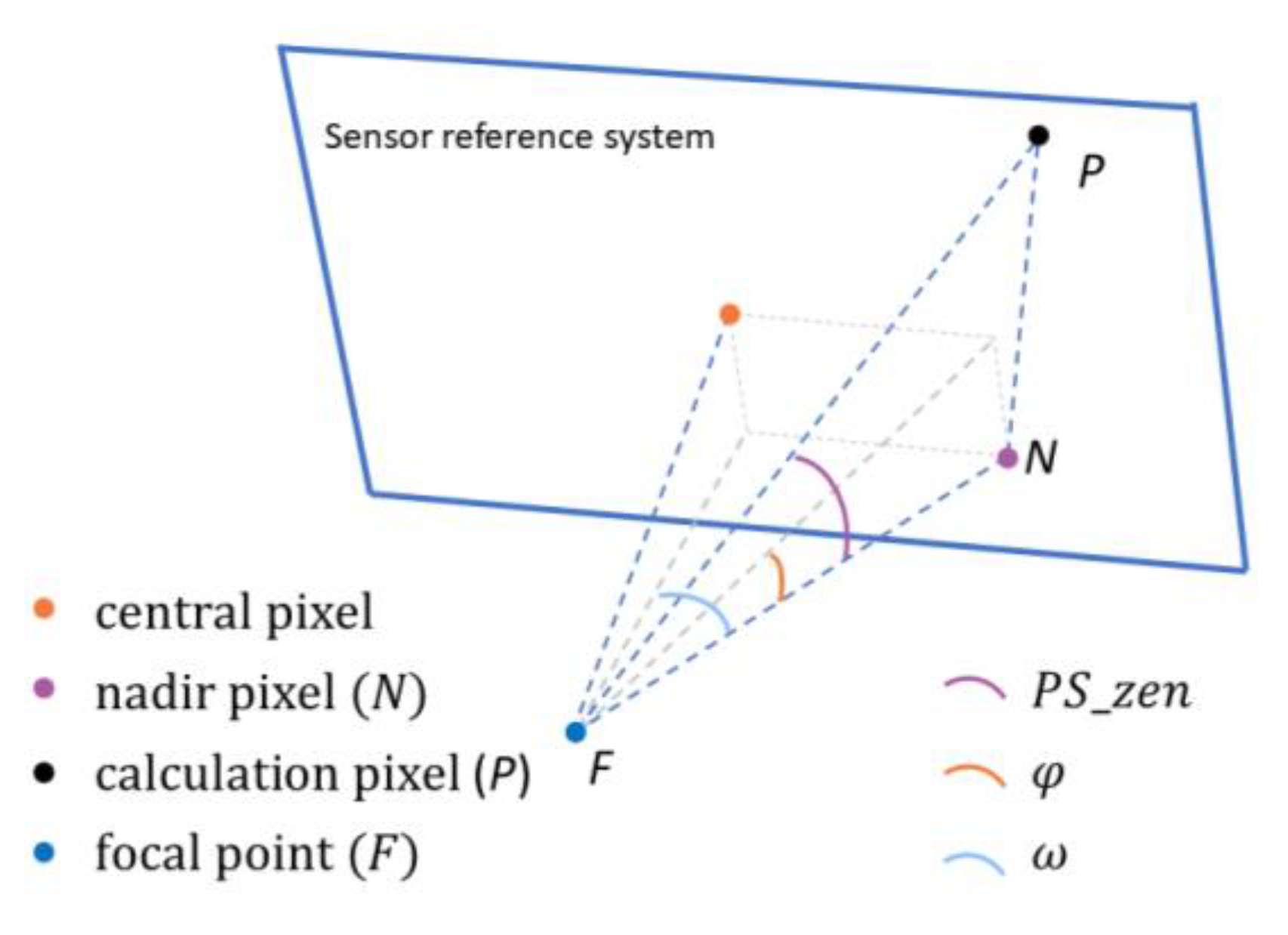
For model calibration, and to isolate the effects of directional reflectance on soil images, twelve flights (indicated in Table 1) were selected for the conjunction of high homogeneity of soil colour, low roughness (seed-bed conditions), and low/no slope. Within the image dataset of each flight, a subset of about 25–30 images (per spectral band) shot from the centre of each field was selected to obtain images exclusively representing flat, homogeneous, bare soil. These images served as the model calibration dataset. Radiometric calibration, vignetting correction, black level compensation and final conversion to reflectance for the Rededge-M images were manually performed, as indicated in the previous chapter. The workflow then proceeded with the identification of the nadir pixels (Figure 2) and the calculation of their relative sensor and sun angles (Figure 3). For each image, the distance in pixel units between the image optical centre (provided by the manufacturer factory calibration) and the pixel coordinates representing the surface point where the sensor was at the nadir position were calculated as Equations (1) and (2):
where u is the pixel column number, v the pixel row number, F the camera focal distance in pixel unit, φ the adjusted sensor Y orientation, ω the adjusted X sensor orientation. This allowed to locate the nadir pixel coordinates (Figure 2). The ANIF map for each image was then calculated as the ratio between average reflectance in a 5 degree diameter around the nadir and each other pixel. The adjusted sensor azimuth κ and the solar azimuth from R solar almanac package “suncalc” [20] were then used to calculate, for each image, the map of the relative azimuth (Figure 3) between each image pixel, the nadir pixel, and the sun azimuth (Rel_az). Relative azimuths were calculated in a 0–180 degree reference system with 0 degrees coinciding with the direction of the solar rays and 180 degrees opposing the sun. The sensor zenith angle (PS_zen) was calculated as the angle between each pixel, the focal point, and the nadir pixel by applying the law of cosines in Equation (3):
from the reference system of the internal camera parameters, where FP is the distance between the focal point and each pixel, FN the distance between the focal point and the nadir, and NP the distance between the nadir pixel and each other pixel (all distances in pixel units). Finally, image maps of the relative sensor-pixel-sun zenith (Rel_zen) was then calculated as Equation (4):
where Sol_zen is the solar zenith from the solar almanac, calculated from the vertical.
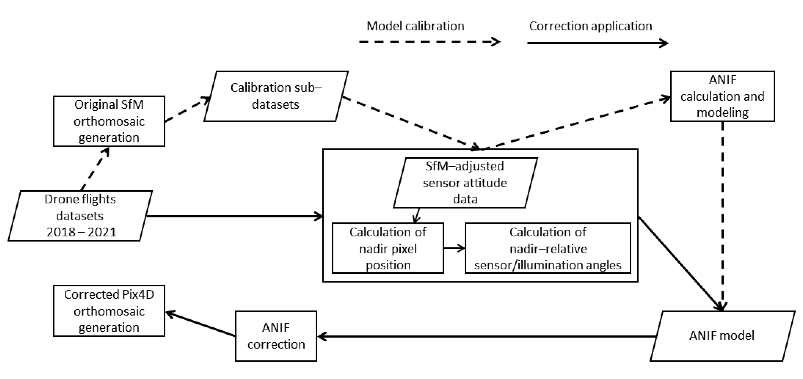
From the maps obtained in the image calibration dataset, the ANIF values were extracted and analysed in correlation to Rel_az, Rel_zen and PS_zen values. The calibration data from the 12 selected flights were merged to represent the entire available range of hemispherical illumination and observation angles (1000 regularly distributed ANIF values per dataset, for a total of 12,000 calibration values). Based on the observed relationships, several model equations with different combinations of input angles were tested and compared for the best ANIF prediction. The performance of the best model was then assessed in the calibration procedure and subsequently on three validation datasets (1000 regularly distributed ANIF values per dataset, for a total of 3000 calibration values), obtained in the same way as for the calibration dataset. R2, Root Mean Square Error (RMSE) and Mean Relative Error % (MRE) were used as model fit evaluators. The general workflow adopted for the calibration and application of the ANIF correction is presented in Figure 4.
2.4. Correction Evaluation
The optimal ANIF correction model was then applied to all available datasets, where the datasets that were not used for calibration were used for validation (distinction marked in Table 1, last column). Images were first converted to reflectance, then Rel_zen and PS_zen angles were calculated to predict and apply the ANIF. The corrected images were then used in PIX4Dmapper for corrected orthomosaic generation, bypassing the camera radiometric calibration and reflectance calculation routine provided in the software. Two steps of correction evaluation were then executed: the first (i) on the images of both calibration and validation datasets, the second (ii) on a subset of orthomosaics, selected visually, which showed distinct “striping” effects (indicated with an * in Table 1 names).
During step (i), to quantify the efficacy of reflectance normalization at the image level, the change in reflectance of the same pixel location coordinates observed from different contiguous images (overlapping FOV but with different shooting time, position, and orientation) was studied before and after correction application. This was accomplished by selecting a set of 220 sample pixels from the orthomosaics of the calibration dataset (12 flights) and 80 sample pixels from the validation dataset (three flights) and tracking their corresponding pixel in all their “parent” images. Between 8 and 20 parent images were identified per pixel sample. The standard deviation (sd) of the reflectance of these parent pixels across different images was then compared between original and corrected images datasets. A substantial reduction in standard deviation after correction is then assumed as indicative for an efficient ANIF correction.
In step (ii), to quantify the “striping” effect in each orthomosaic, before and after the correction, spectral data were extracted from 8–10 transects positioned perpendicularly to the stripes. In this way, the stripes were expected to appear as spectral peaks and valleys along the transects. The positions of the drone flight lines were then overlaid on the transects, and this made it possible to study the magnitude of the striping effect in relation to the flight line positions. Two indexes were then extracted: a “spectral sinuosity” index (SSin), and the correlation between the magnitude of spectral peaks/valleys and the distance from the drone flight lines. SSin was calculated as Equation (5):
where N is the number of pixels along the transect, the pixel index along the transect, the reflectance (0–100 scale) and the average pixel length on the transect (m). It is the ratio between the transect distance weighted by its pixel-by-pixel spectral variability and the real planimetric distance, with domain SSin ≥ 1, where the minimum value of 1 means no spectral variability across transect distance. The average SSin of all transects of a map is then calculated.
To calculate the correlation between striping and distance from the flight lines, the magnitude of the peaks/valleys was associated to the residuals of a linear interpolation of the reflectance values along each transect. The correlation was then calculated between these residuals and the horizontal distance to the closest flight line. The underlying assumption is that, in an ideal multispectral image dataset free of anisotropic effects, reflectance changes should not show correlation with distance from the image capture positions.
3. Results
3.1. Striping Issue
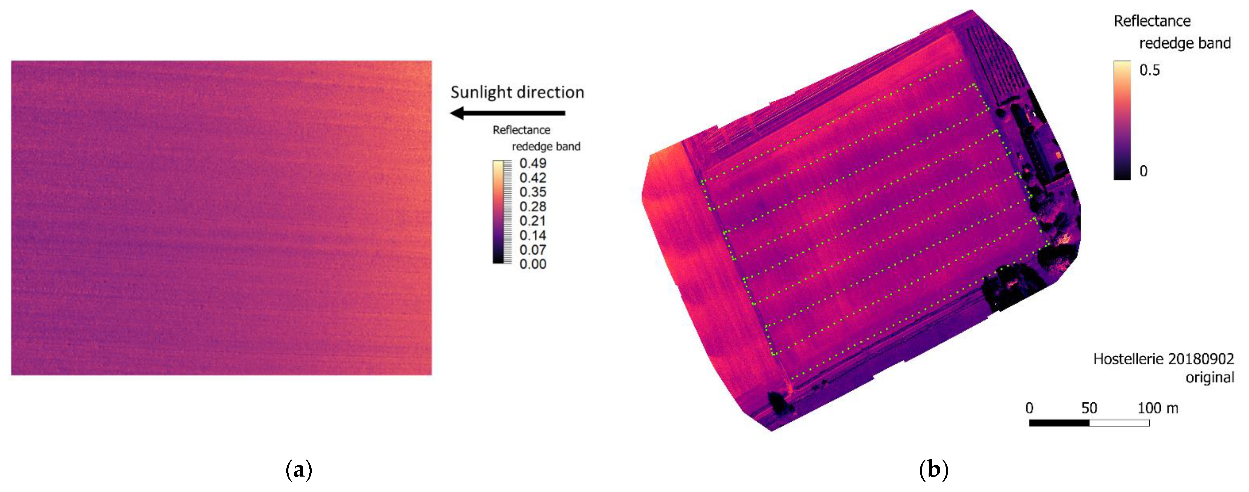
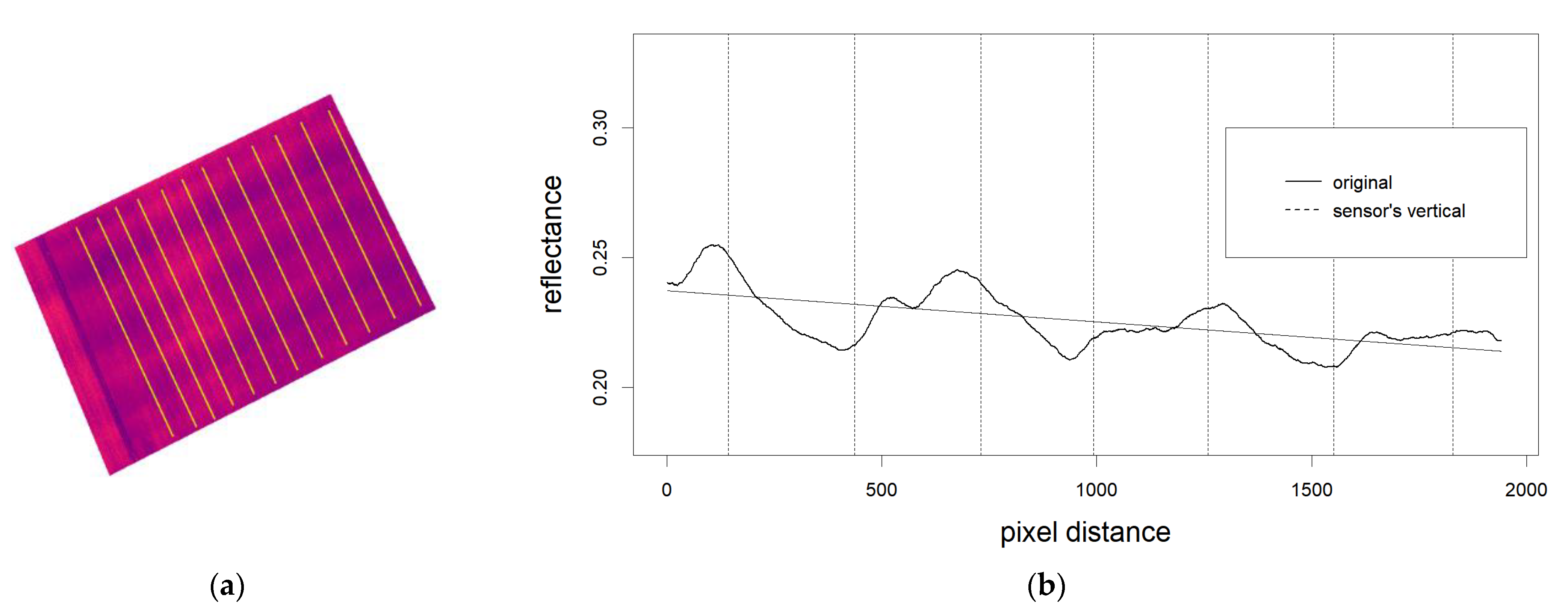
The effects of soil reflectance anisotropy on the products of our UAS-based multispectral survey were evident both in the images and in the final products of the photogrammetric orthomosaic reconstruction. A spectral gradient in apparent correlation with the direction of incoming sunlight was evident in all the images (e.g., in Figure 5a), in accordance with previous observations on the differences between the forward- and back-scattering reflectance of soil surfaces [21,22,23,24]. With the camera tilted forward in a fixed position to constantly aim at the nadir during cruising speed, this spectral gradient was invariant from the changing drone heading. We therefore excluded any other major systematic effect on measured reflectance (i.e., due to the camera orientation) than illumination direction. The combination of this systematic gradient behaviour and the regular geometry of the flight lines used for the image acquisition resulted in spectral artefacts in the final products of the photogrammetric orthomosaic reconstruction. These artefacts (example presented in Figure 5b) manifested as stripes with different spectral intensities, parallel and in concomitance with flight lines. When observed along transects perpendicular to the flight lines (e.g., in Figure 6a), these stripes took the form of spectral peaks and valleys (e.g., in Figure 6b).
3.2. Model Fit
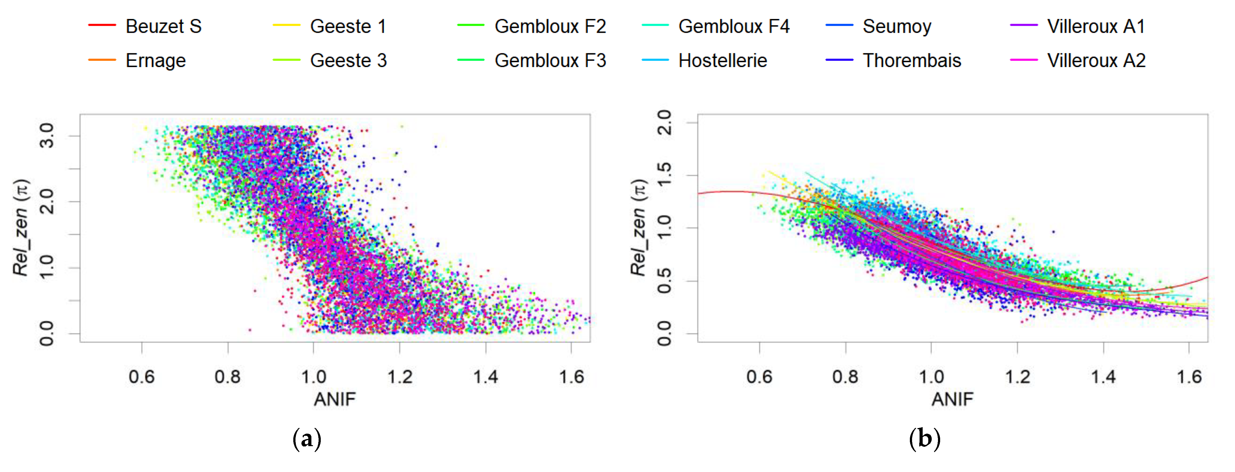
The results of the calibration data extraction are summarized in Figure 7, where the correlation plots show that both Rel_az and Rel_zen exhibited a stable behaviour with the ANIF across all the sampled conditions of solar illumination. Different equation arrangements of the Rel_az, Rel_zen, and PS_zen angles were tested for their overall ANIF prediction capability and for their image correction capability. The chosen form of the final model was Equation (6):
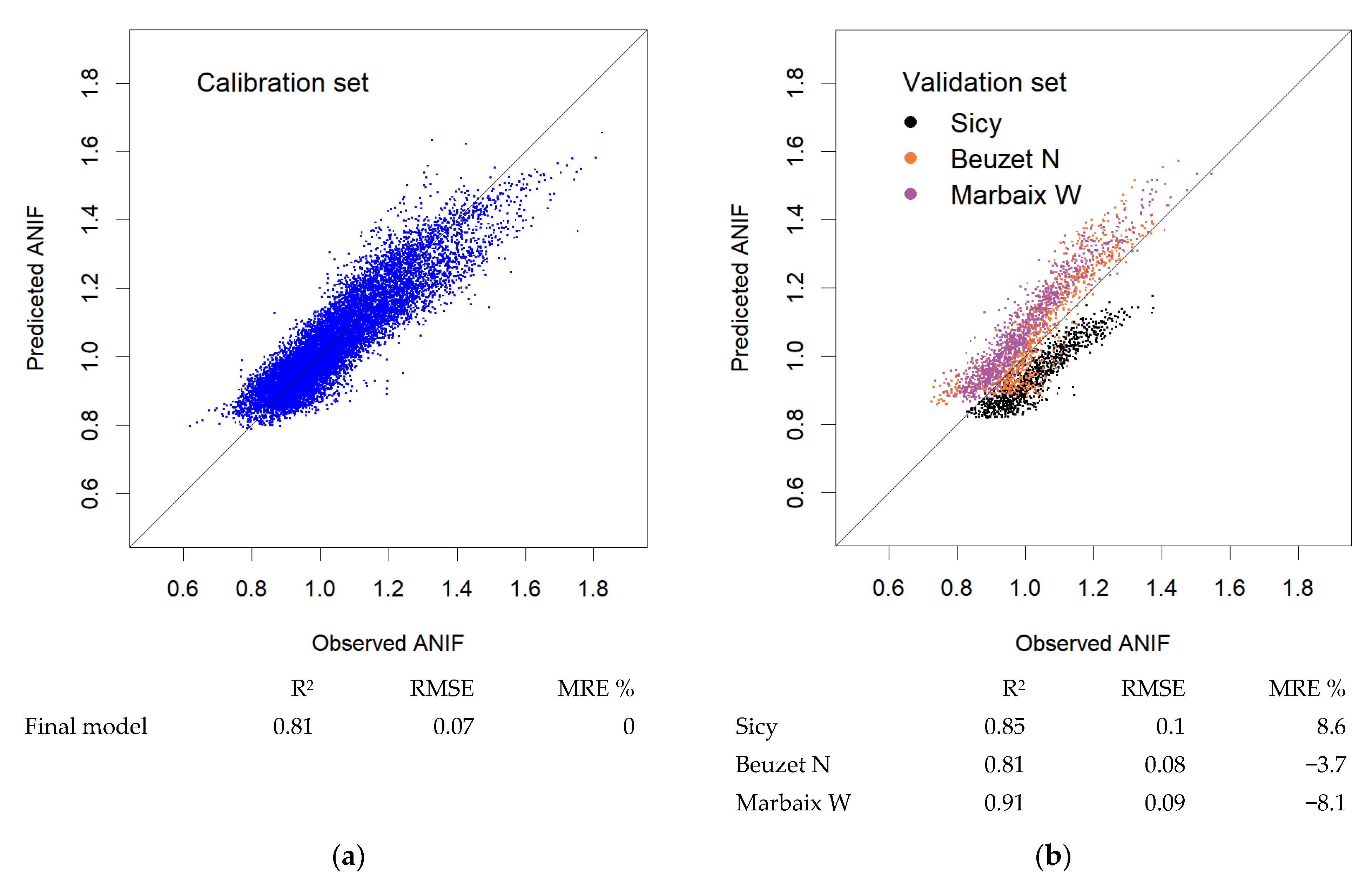
with a, b, c, and d being the regression coefficients. The model was chosen for its high fit (R2 = 0.81, RMSE = 0.07, MRE = 0% in Figure 8a) and after the assessment of the absence of artefacts in the corrected images, and of the “flattening” of the spectral value across the image field. The spectral “flattening” was visually examined through spectral data extraction in transects, as shown in Figure 9, in a subset of two images per calibration set (2 × 12). The model was tested on the three validation datasets, providing the results summarized in Figure 8b. The validation results showed that the model seems to provide stable and consistent ANIF predictions across the tested observation/illumination range (0.81 < R2 < 0.91, 0.08 < RMSE < 0.1) but with a dataset-dependent bias, showed by a noticeable positive or negative MRE (%) and evident in the observed vs. predicted plot (Figure 8b).
ANIF ~ a∙Rel_zen1 + b∙Rel_zen2 + c∙Rel_zen3 + d∙PS_zen
3.3. Correction Evaluation Results
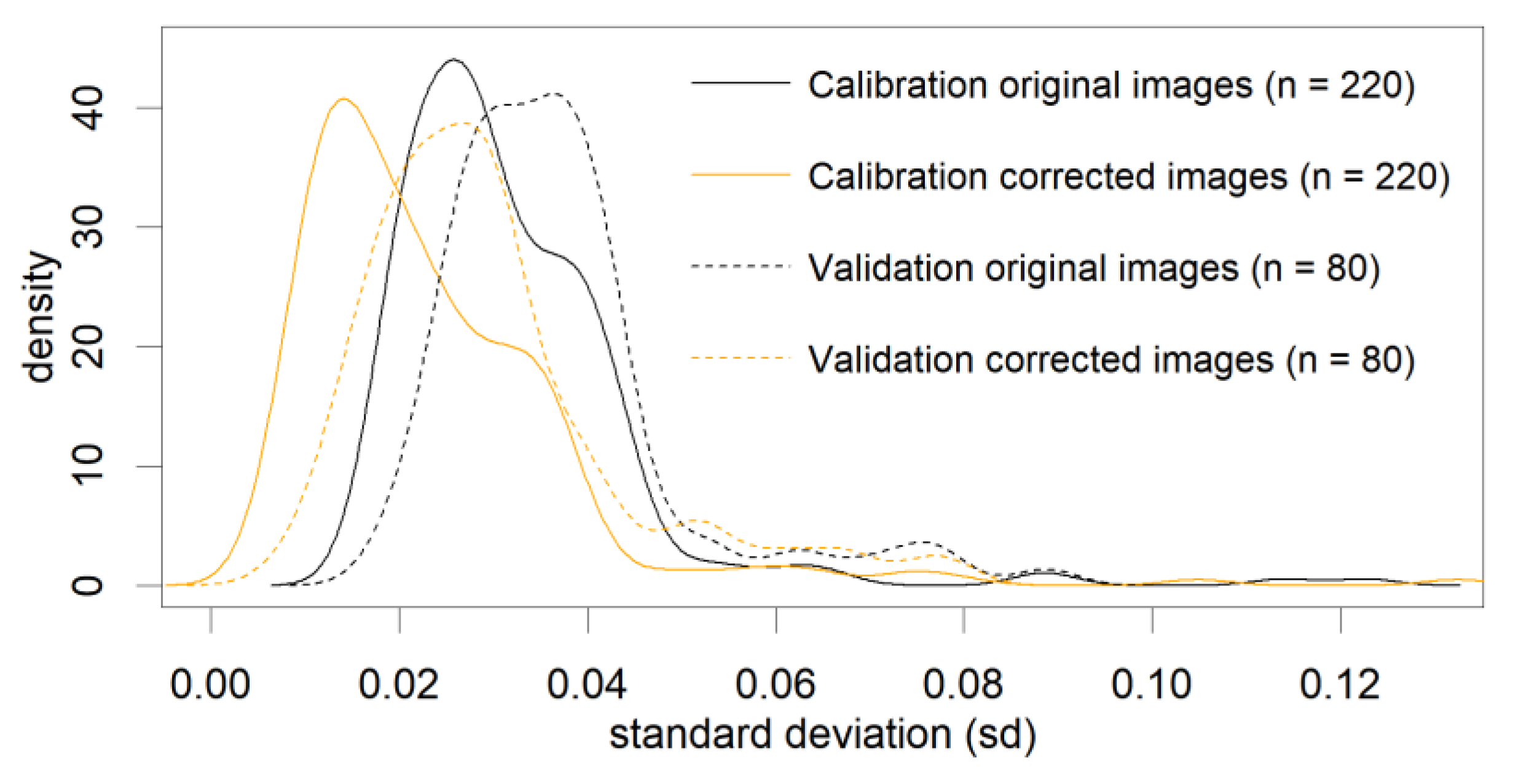
Step (i) of our analysis showed that, on average, the measurement of the same pixel location from different images was more spectrally stable after the proposed ANIF correction. In the calibration dataset, the standard deviation of the measured sample pixel reflectance from the corrected images (mean = 0.023) was indeed lower (t [429] = 6.03, p < 0.05) than in the original images (mean = 0.032). This is also supported by a comparison of the density plots before and after correction (Figure 10). A comparable result was also obtained with the validation dataset (density plots in Figure 10), were the sd of reflectance in the corrected images (mean = 0.030) was significantly lower (t [172] = 3.58, p < 0.05) than with the original images (mean = 0.037). The reflectance stability of the validation set was generally lower (corrected images obtained the same mean and sd density distribution as the original images in the calibration dataset) but the starting conditions were also worse (starting from an sd of 0.037).
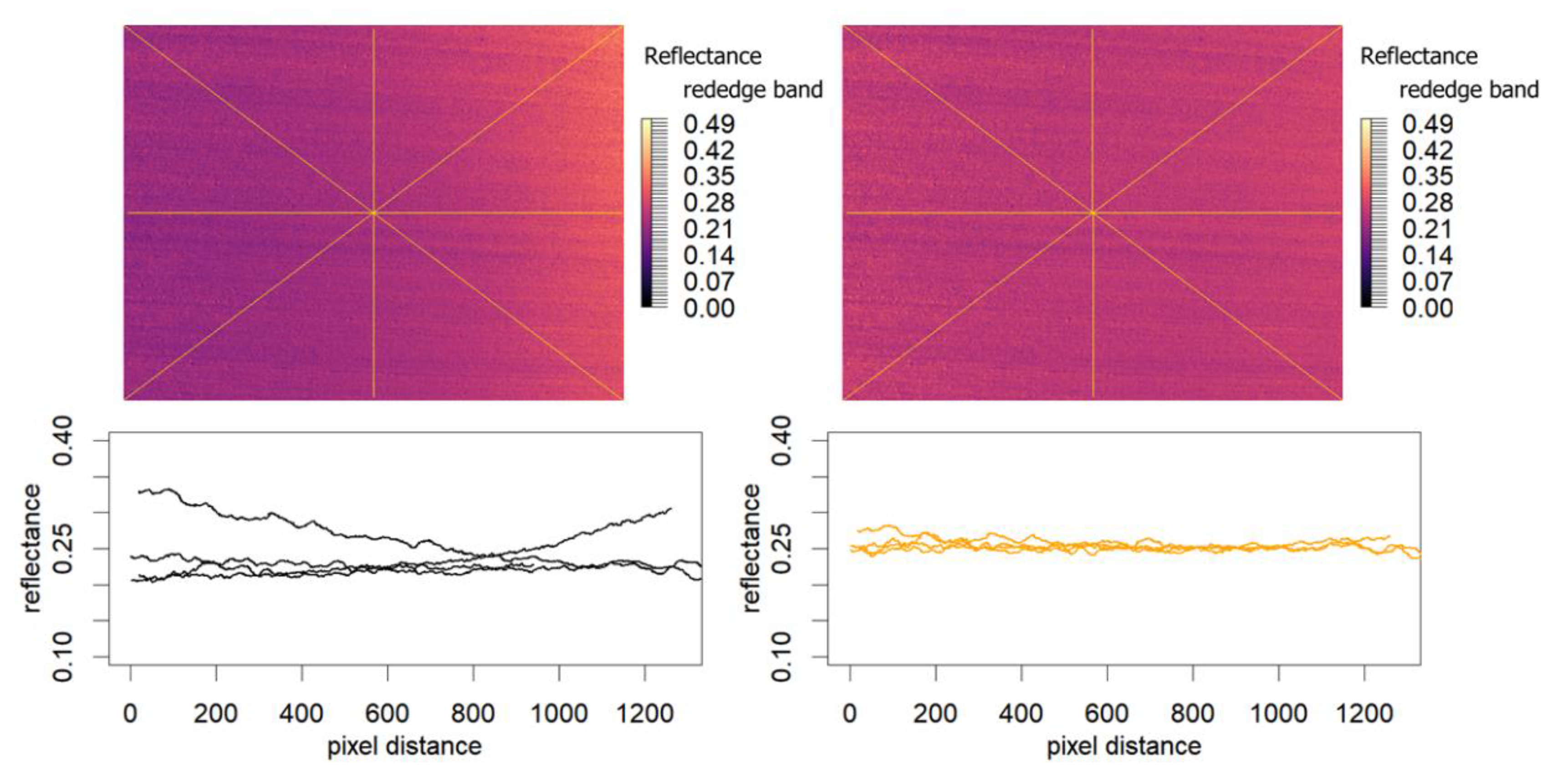
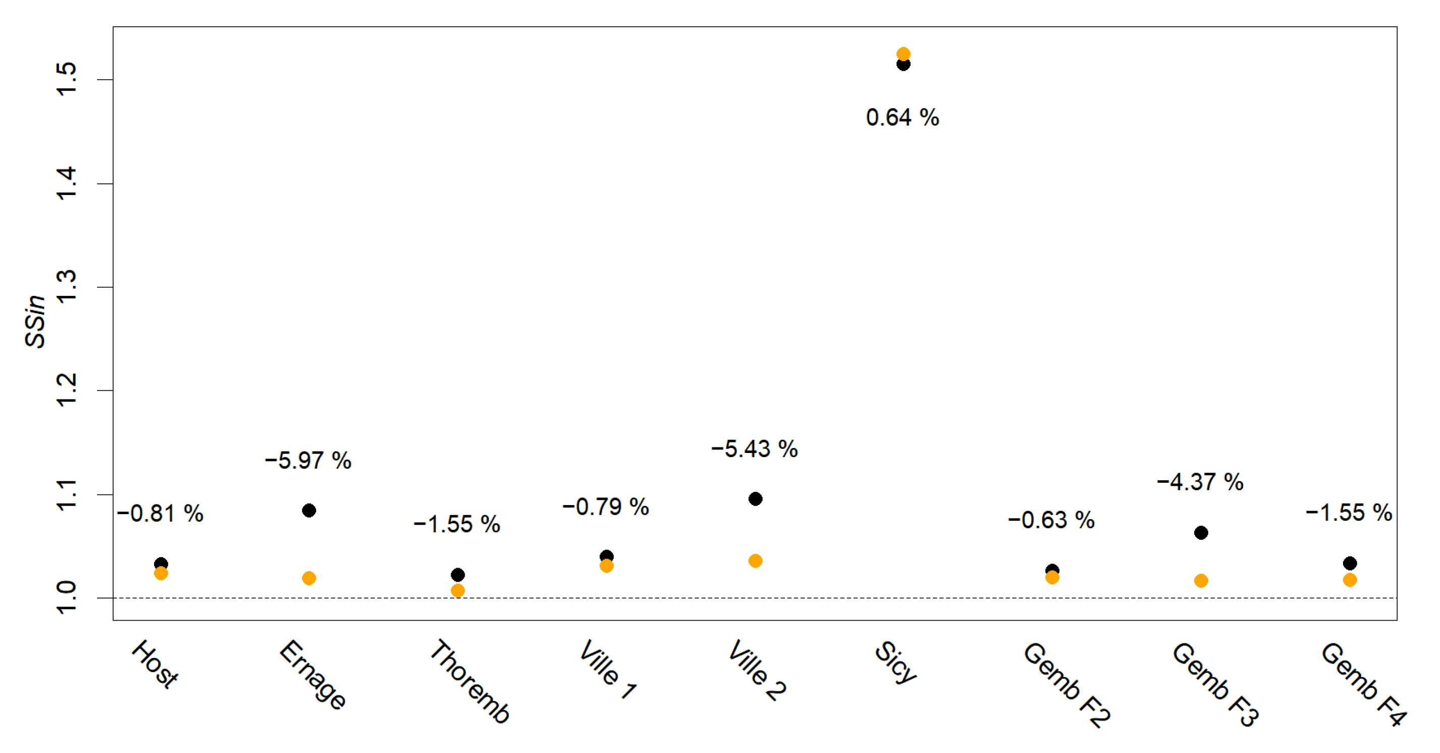
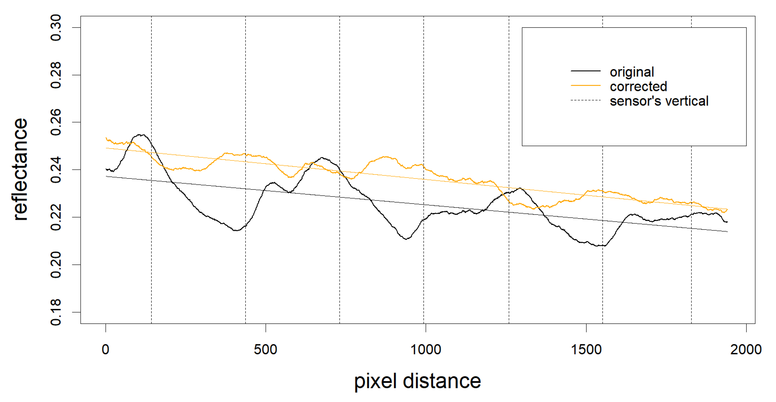
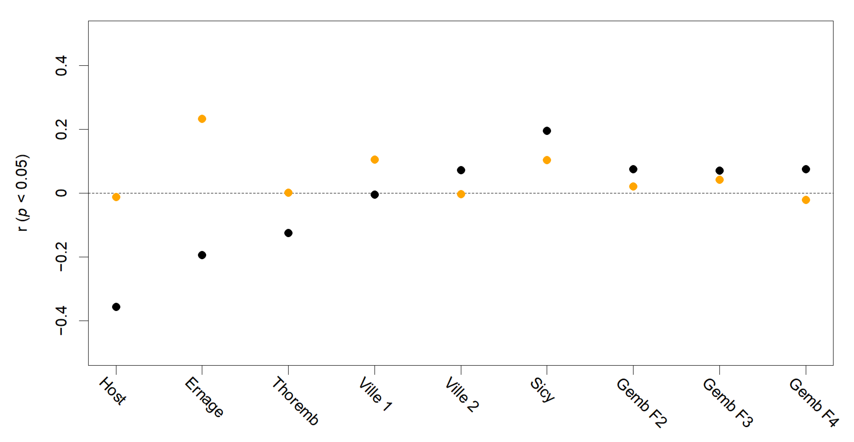
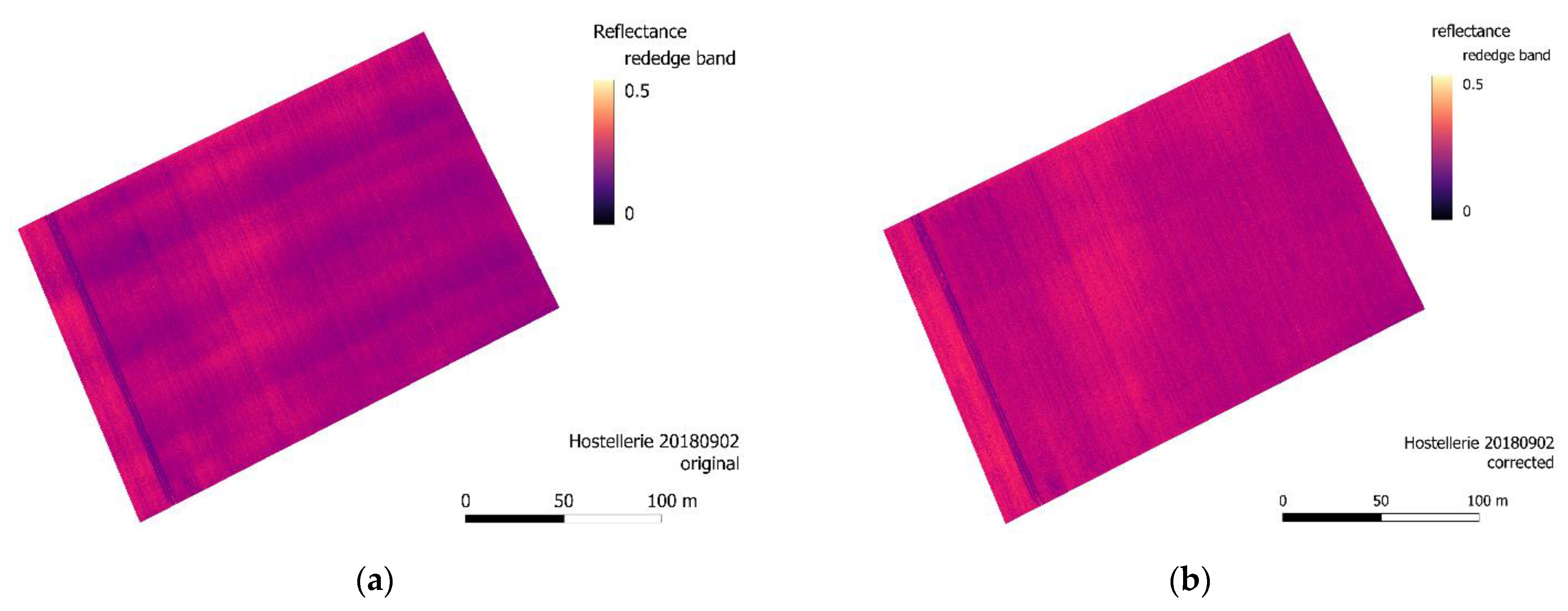
Regarding the evaluation step (ii), the average SSin index calculated for the nine selected sets (Figure 11) decreased in all cases except one (“Sicy”), showing that with the proposed correction, the sinuosity is generally reduced by a minimum of 0.63% to a maximum of 5.97%. A visual SSin reference example can be found in Figure 12, where the original and corrected transect provided SSin values of 1.030 and 1.022, respectively, with a decrease in sinuosity of 0.77%. Without a clear reference sinuosity index to discriminate between a map affected by stripes and a corrected map, apart from a visual interpretation, an analysis of the spectral data in relation to the drone flight lines was carried out to support the positive effects of our correction methodology. The correlation between the magnitude of the spectral peaks and valleys on the transect and the distance to the closest flight line (sensor position) is provided in Figure 13 for the nine selected datasets. Generally, a higher correlation (both positive and negative) was observed in the original maps, where the peaks and/or valleys of the stripes seem to be either very close (as per the example in Figure 12) or very far from the flight lines. On the other hand, a weaker or zero correlation was generally observed on the corrected maps. The position of the sensor in the presence of the stripes did not show consistent behaviour: in some cases, both peaks and valleys were associated with high proximity to the flight lines, resulting in an overall negative correlation; in other cases, only peaks or only valleys were close to the flight lines, resulting in either a positive or negative correlation, depending on the local transect linear interpolation. In general, a lower correlation associated with the corrected orthomosaics indicated that the striping effect was effectively eliminated in most cases and at least reduced in some others. As a visual example of the difference between the original and the corrected spectral orthomosaic (e.g., rededge band) and of the elimination of the “striping” effect, the orthomosaic product of the “Hostellerie” dataset is reported in Figure 14.
4. Discussion
The results of analysis step (i) showed that the stability of the spectral measurement of the same pixel location across different images sensibly improved after the application of the ANIF correction. The relative improvement in sd (Figure 10) was almost the same for the calibration and validation datasets, although the overall spectral stability was lower in the validation dataset. This was probably due to the non-optimal terrain conditions that prevented the initial choice of the three validation datasets for calibration purposes. Contrary to the calibration dataset, the fields used for the validation data were characterized by non-homogeneous soil colours, soil crusting (accumulation on the surface of finer particles with high reflectance), vegetation residue and varying slope/aspect. In this regard, the effects of the soil colour and vegetation residuals could probably be encompassed by a richer calibration sampling. On the other hand, surface slope and aspect play much more important roles in illumination geometry, which are generally tackled with topographic correction methods [25,26], but their effect on soil anisotropy was not accounted for in the context of this research. The specific ANIF model equation in this study was developed using only relative observation/illumination angles, which are slope/aspect-invariant and only dependent on sensor and sun orientation. This represents a limitation and calls for further development of the proposed model. Moreover, the surface roughness and the partial or total loss of radiometric signature caused by its shadows represent additional issues in need of further scrutiny [27,28,29].
The two correction evaluation indicators adopted in step (ii) seem to show that, in general, the specific “striping” artefact affecting the orthomosaics of the available dataset was greatly reduced or eliminated following the proposed correction methodology. Some uncertainties arose, such as the observation of the SSin analysis results (Figure 13), which revealed the anomaly of higher SSin values in the “Sicy” dataset compared to the other fields. For this specific case, it must be noted that the dataset was not used in model calibration as its images were not sufficiently homogeneous due to the prominent presence of tractor tracks in most of the images. Therefore, the interpretation of step (ii) indexes was confined to this specific case study, as no other studies were found to tackle this specific problem, and no proper comparison with other indicators could be drawn. Moreover, we could not present completely objective evaluations of the correctness of the analysed spectral orthomosaics, as no independent data with reference methods were available.
5. Conclusions
This study provided an empirical correction methodology for UAS-based multispectral imaging datasets of bare soils to account for the effects of the BRDF, based on the application of an anisotropy factor (ANIF) correction. The dataset of the images available for this study was sufficient to calibrate a simple model relating the ANIF to a wide range of sensor-pixel-illumination conditions by using only two angles: relative sensor-pixel-sun zenith and relative sensor-pixel-sun azimuth. The proposed correction was tested on 15 available datasets. As a result, the employment of ANIF-corrected images for multispectral orthomosaic generation with photogrammetric software provided spectral maps free of anisotropic-related artefacts in most cases, as assessed by several ad hoc indexes. The validation with an independent image dataset, however, showed the presence of some systematic errors, the causes of which require further investigation. Plausible future directions for model enhancement include the implementation of a topographic index to account for the effects of slope and aspect, the consideration of soil roughness and its related shadows, and/or an enrichment of the model calibration with different soil conditions (vegetation residue, humidity, crusting).
Author Contributions
Conceptualization, K.V.O., K.P. and G.C.; methodology, G.C. and H.Z.; software, G.C. and H.Z.; validation, G.C. and H.Z.; formal analysis, G.C.; investigation, G.C. and H.Z.; resources, K.V.O.; data curation, G.C. and H.Z.; writing—original draft preparation, G.C. and H.Z.; writing—review and editing, G.C., K.V.O. and K.P.; visualization, G.C.; supervision, K.V.O. and K.P.; project administration, K.V.O.; funding acquisition, K.V.O. All authors have read and agreed to the published version of the manuscript.
Funding
This research was funded by: (i) the Belgian Federal Science Policy Office, BELSPO STEREO project SR/10/202 “MS—SOC”; (ii) the Fund for Scientific Research—Belgium: F 3/5/5—FRIA/FC—12691.
Institutional Review Board Statement
Not applicable.
Informed Consent Statement
Not applicable.
Data Availability Statement
The scripts and model parameters used in this study are available in a publicly accessible repository that does not issue DOIs. These data can be found here: https://github.com/Debrisman/Micasense_Rededge_correction, accessed on 20 December 2021.
Acknowledgments
Giacomo Crucil is an ASP of the Fonds de la Recherche Scientifique (FNRS)—Fonds pour la formation à la Recherche dans l’Industrie et dans l’Agriculture (FRIA).
Conflicts of Interest
The authors declare no conflict of interest.
References
- Viscarra Rossel, R.A.; Walvoort, D.J.J.; McBratney, A.B.; Janik, L.J.; Skjemstad, J.O. Visible, near infrared, mid infrared or combined diffuse reflectance spectroscopy for simultaneous assessment of various soil properties. Geoderma 2006, 131, 59–75. [Google Scholar] [CrossRef]
- Ben-Dor, E. Soil spectral imaging: Moving from proximal sensing to spatial quantitative domain. ISPRS Ann. Photogramm. Remote Sens. Spat. Inf. Sci. 2012, 1, 67–70. [Google Scholar]
- Colomina, I.; Molina, P. Unmanned aerial systems for photogrammetry and remote sensing: A review. ISPRS J. Photogramm. Remote Sens. 2014, 92, 79–97. [Google Scholar] [CrossRef] [Green Version]
- Soriano-Disla, J.M.; Janik, L.J.; Allen, D.J.; McLaughlin, M.J. Evaluation of the performance of portable visible-infrared instruments for the prediction of soil properties. Biosyst. Eng. 2017, 161, 24–36. [Google Scholar] [CrossRef]
- Aldana-Jague, E.; Heckrath, G.; Macdonald, A.; van Wesemael, B.; Van Oost, K. UAS-based soil carbon mapping using VIS-NIR (480–1000 nm) multi-spectral imaging: Potential and limitations. Geoderma 2016, 275, 55–66. [Google Scholar] [CrossRef]
- Menzies Pluer, E.G.; Robinson, D.T.; Meinen, B.U.; Macrae, M.L. Pairing soil sampling with very-high resolution UAV imagery: An examination of drivers of soil and nutrient movement and agricultural productivity in southern Ontario. Geoderma 2020, 379, 114630. [Google Scholar] [CrossRef]
- Wehrhan, M.; Rauneker, P.; Sommer, M. UAV-based estimation of carbon exports from heterogeneous soil landscapes—A case study from the carboZALF experimental area. Sensors 2016, 16, 255. [Google Scholar] [CrossRef] [Green Version]
- Aasen, H.; Honkavaara, E.; Lucieer, A.; Zarco-Tejada, P.J. Quantitative remote sensing at ultra-high resolution with UAV spectroscopy: A review of sensor technology, measurement procedures, and data correctionworkflows. Remote Sens. 2018, 10, 1091. [Google Scholar] [CrossRef] [Green Version]
- Nicodemus, F. Book Reviews. J. Opt. Soc. Am. 1977, 67, 127–130. [Google Scholar]
- Beisl, U. Correction of Bidirectional Effects in Imaging Spectrometer Data; Remote Sensing Series 37; Zurich: Hong Kong, China, 2001; ISBN 3037030011. [Google Scholar]
- Roosjen, P.P.J.; Suomalainen, J.M.; Bartholomeus, H.M.; Kooistra, L.; Clevers, J.G.P.W. Mapping reflectance anisotropy of a potato canopy using aerial images acquired with an unmanned aerial vehicle. Remote Sens. 2017, 9, 417. [Google Scholar] [CrossRef] [Green Version]
- Aasen, H.; Bolten, A. Multi-temporal high-resolution imaging spectroscopy with hyperspectral 2D imagers–From theory to application. Remote Sens. Environ. 2018, 205, 374–389. [Google Scholar] [CrossRef]
- Schlapfer, D.; Richter, R.; Feingersh, T. Operational BRDF effects correction for wide-field-of-view optical scanners (BREFCOR). IEEE Trans. Geosci. Remote Sens. 2015, 53, 1855–1864. [Google Scholar] [CrossRef] [Green Version]
- Sandmeier, S.; Müller, C.; Hosgood, B.; Andreoli, G. Sensitivity analysis and quality assessment of laboratory BRDF data. Remote Sens. Environ. 1998, 64, 176–191. [Google Scholar] [CrossRef]
- SZ DJI Technology Co., Ltd. Shenzhen, China. Version 2.0.15; 2018. Available online: https://www.dji.com/it/downloads/products/ground-station-pro (accessed on 1 February 2018).
- Pix4Dmapper SA. Prilly, Switzerland. Version 4.4.12; 2021. Available online: https://pix4d.com/product/pix4dmapper-photogrammetry-software (accessed on 1 April 2020).
- RedEdge Camera Radiometric Calibration Model. Available online: https://support.micasense.com/hc/en-us/articles/115000351194-Rededge-Camera-Radiometric-Calibration-Model (accessed on 8 February 2020).
- R Core Team. R: A Language and Environment for Statistical Computing; Version 3.6.3; R Foundation for Statistical Computing: Vienna, Austria, 2021; Available online: https://www.R-project.org (accessed on 1 February 2020).
- Schaepman-Strub, G.; Painter, T.; Huber, S.; Dangel, S.; Schaepman, M.E.; Martonchik, J.; Berendse, F. About the importance of the definition of reflectance quantities—Results of case studies. Int. Arch. Photogramm. Remote Sens. Spat. Inf. Sci.—ISPRS Arch. 2004, 35, 361–366. [Google Scholar]
- Benoit Thieurmel and Achraf Elmarhraoui. Suncalc: Compute Sun Position, Sunlight Phases, Moon Position and Lunar Phase; R Package Version 0.5.0; 2019. Available online: https://cran.r-project.org/web/packages/suncalc (accessed on 1 May 2020).
- Brennan, B.; Bandeen, W.R. Anisotropic reflectance characteristics of natural earth surfaces. Appl. Opt. 1970, 9, 405–412. [Google Scholar] [CrossRef]
- Milton, E.J.; Webb, J.P. Ground radiometry and airborne multispectral survey of bare soils. Int. J. Remote Sens. 1987, 8, 3–14. [Google Scholar] [CrossRef]
- Croft, H.; Anderson, K.; Kuhn, N.J. Reflectance anisotropy for measuring soil surface roughness of multiple soil types. Catena 2012, 93, 87–96. [Google Scholar] [CrossRef]
- Anderson, K.; Croft, H. Remote sensing of soil surface properties. Prog. Phys. Geogr. 2009, 33, 457–473. [Google Scholar] [CrossRef]
- Richter, R.; Kellenberger, T.; Kaufmann, H. Comparison of topographic correction methods. Remote Sens. 2009, 1, 184–196. [Google Scholar] [CrossRef] [Green Version]
- Jakob, S.; Zimmermann, R.; Gloaguen, R. The Need for accurate geometric and radiometric corrections of drone-borne hyperspectral data for mineral exploration: MEPHySTo-A toolbox for pre-processing drone-borne hyperspectral data. Remote Sens. 2017, 9, 88. [Google Scholar] [CrossRef] [Green Version]
- Crucil, G.; Van Oost, K. Towards mapping of soil crust using multispectral imaging. Sensors 2021, 21, 1850. [Google Scholar] [CrossRef] [PubMed]
- Movia, A.; Beinat, A.; Crosilla, F. Shadow detection and removal in RGB VHR images for land use unsupervised classification. ISPRS J. Photogramm. Remote Sens. 2016, 119, 485–495. [Google Scholar] [CrossRef]
- Croft, H.; Anderson, K.; Kuhn, N.J. Evaluating the influence of surface soil moisture and soil surface roughness on optical directional reflectance factors. Eur. J. Soil Sci. 2014, 65, 605–612. [Google Scholar] [CrossRef]
Figure 1.
Field locations contextualized within Belgian border (a), and in more detail within the Belgian loam belt area (c), of the UAS flights used in this study. A close-up example of soil conditions is reported in frame (b).
Figure 1.
Field locations contextualized within Belgian border (a), and in more detail within the Belgian loam belt area (c), of the UAS flights used in this study. A close-up example of soil conditions is reported in frame (b).

Figure 2.
Scheme for the calculation of the pixel nadir coordinates and of the sensor zenith relative to the nadir “PS_zen” angle in a tilted (by pitch and roll angles) sensor reference system.
Figure 2.
Scheme for the calculation of the pixel nadir coordinates and of the sensor zenith relative to the nadir “PS_zen” angle in a tilted (by pitch and roll angles) sensor reference system.

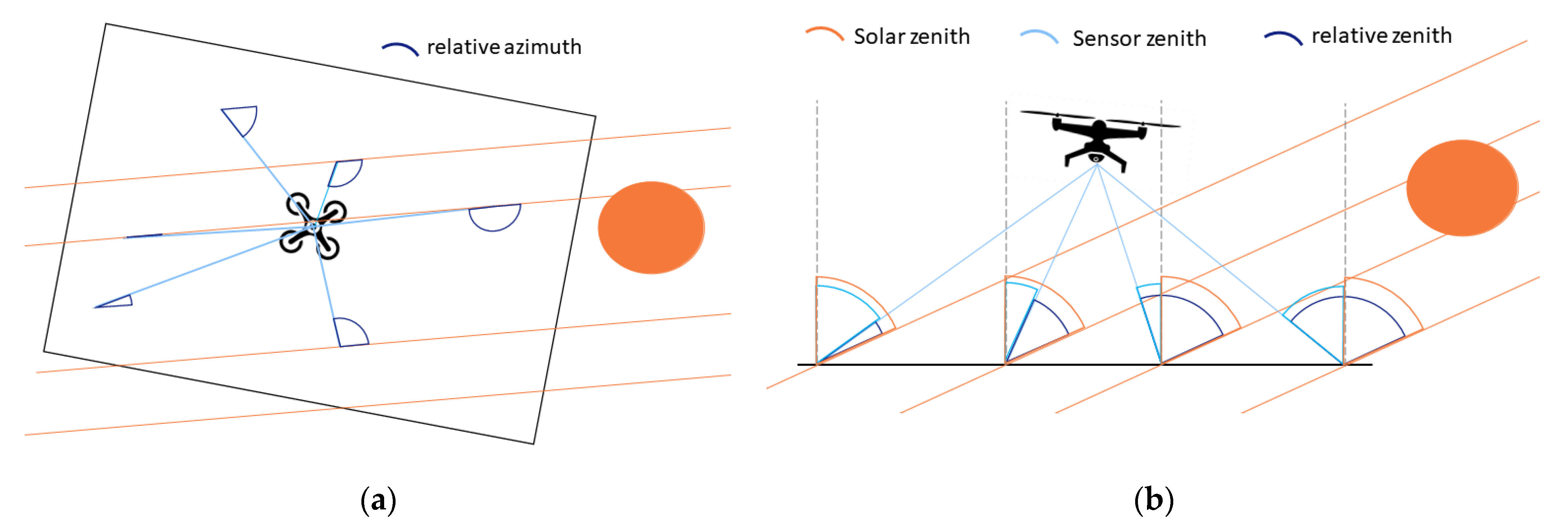
Figure 3.
Visualization of the relative angles extracted for BRDF modelling within the sun-pixel-sensor framework: (a) relative azimuth “Rel_az”; (b) sensor zenith “PS_zen”, solar zenith “Sol_zen”, relative zenith “Rel_zen”.
Figure 3.
Visualization of the relative angles extracted for BRDF modelling within the sun-pixel-sensor framework: (a) relative azimuth “Rel_az”; (b) sensor zenith “PS_zen”, solar zenith “Sol_zen”, relative zenith “Rel_zen”.

Figure 4.
Workflow for ANIF model calibration and application.

Figure 5.
(a) Example of Micasense Rededge-M picture of flat soil, shot from 45 m above ground level, after manual radiometric calibration, vignetting correction, black-level compensation and conversion to reflectance. The rededge band is used as example in order to show how it is affected by reflectance gradient due to back- and forward-scattering effects of incoming sunlight; (b) example of PIX4Dmapper-generated spectral orthomosaic (rededge band as example) obtained from a dataset of images non corrected for the soil anisotropy effects. The image positions, along the flight lines, are presented (green dots) to show their correspondence with the “stripes” artefact. The rededge band was arbitrarily chosen for display purposes only, as all spectral bands exhibited the same behaviour.

Figure 6.
(a) Example of transect drawing on a map affected by the stripes artefact; (b) example of transect spectral data, from the original dataset, and the corresponding linear interpolation. The position of flight lines (sensor vertical position) is indicated as black dashed lines.
Figure 6.
(a) Example of transect drawing on a map affected by the stripes artefact; (b) example of transect spectral data, from the original dataset, and the corresponding linear interpolation. The position of flight lines (sensor vertical position) is indicated as black dashed lines.

Figure 7.
From a subsampling of the ensemble of the 12 calibration datasets: (a) correlation plot of Rel_az (in radians) against the ANIF; (b) correlation plot of Rel_zen (in radians) against the ANIF, with the 3rd order polynomial interpolation lines from the different datasets.
Figure 7.
From a subsampling of the ensemble of the 12 calibration datasets: (a) correlation plot of Rel_az (in radians) against the ANIF; (b) correlation plot of Rel_zen (in radians) against the ANIF, with the 3rd order polynomial interpolation lines from the different datasets.

Figure 8.
Observed vs. predicted plot of the ANIF from the modelling of the calibration (a) and validation (b) datasets. R2, root mean square error (RMSE) and mean relative error % (MRE) are indicated below each respective plot.
Figure 8.
Observed vs. predicted plot of the ANIF from the modelling of the calibration (a) and validation (b) datasets. R2, root mean square error (RMSE) and mean relative error % (MRE) are indicated below each respective plot.

Figure 9.
Example of reflectance picture (rededge band) before (left) and after (right) ANIF correction. The yellow lines represent the transect from which spectral data were extracted to check the result of spectral normalization. The data extracted from the transects are plotted under the respective images, in black for the original image and in orange for the corrected image.

Figure 10.
Results of step (i) analysis: density distribution for a calibration sample size n = 220 and validation sample size n = 80 of the standard deviation sd of reflectance for same pixel observation by different camera positions/angles (9–20 different camera observation per pixel), before and after ANIF correction (black and orange lines, respectively).

Figure 11.
Results of step (ii): average spectral sinuosity index SSin for each field. Black = original orthomosaics, orange = corrected orthomosaics. The % difference between SSin of corrected and original reflectance transects is indicated above each point.
Figure 11.
Results of step (ii): average spectral sinuosity index SSin for each field. Black = original orthomosaics, orange = corrected orthomosaics. The % difference between SSin of corrected and original reflectance transects is indicated above each point.

Figure 12.
Results of step (ii): example of transect spectral data evaluation (Hostellerie dataset), before and after image correction (black and orange, respectively), and the corresponding linear interpolation. The positions of the flight lines (sensor vertical position) are marked as black dashed lines. The SSin calculated for the original transect was 1.030 while that of the corrected transect was 1.022.

Figure 13.
Results of step (ii): correlation between striping magnitude and distance from the vertical of the closest flight line/sensor position, measured across spectral transects.
Figure 13.
Results of step (ii): correlation between striping magnitude and distance from the vertical of the closest flight line/sensor position, measured across spectral transects.

Figure 14.
Example of original (a) and ANIF-corrected (b) final spectral orthomosaic (rededge band example) for the flight Hostellerie 2 September 2018.
Figure 14.
Example of original (a) and ANIF-corrected (b) final spectral orthomosaic (rededge band example) for the flight Hostellerie 2 September 2018.


Table 1.
General flight information of the UAS flight database: name, execution date, lateral overlap %, flight line and sunlight direction and whether the dataset was used for ANIF model calibration or validation. Names marked with an (*) represent datasets that in the original orthomosaic generation phase showed a prominent “striping” artefact effect. Flight altitude was ca. 45 m above ground level in all cases.
| Field Name | Date | Lateral Overlap (%) | Flight Line Azimuth (deg) | Sun Azimuth (deg) | Sun Zenith (deg) | Model Calibration/ Validation |
|---|---|---|---|---|---|---|
| Seumoy | 7 May 2018 | 80 | 60/240 | 220 | 38 | Cal |
| Thorembais * | 7 May 2018 | 75 | 40/220 | 150 | 37 | Cal |
| Beuzet Sud | 8 May 2018 | 75 | 127/307 | 240 | 46 | Cal |
| Hostellerie * | 2 September 2018 | 75 | 65/245 | 140 | 49 | Cal |
| Geeste 1 | 2 September 2018 | 75 | 67/247–147/327 | 160 | 44 | Cal |
| Geeste 3 | 2 September 2018 | 75 | 65/245 | 190 | 43 | Cal |
| Ernage * | 20 April 2019 | 75 | 35/215 | 140 | 44 | Cal |
| Villeroux a1 * | 27 August 2019 | 80 | 45/225 | 200 | 42 | Cal |
| Villeroux a2 * | 14 September 2019 | 80 | 45/225 | 190 | 47 | Cal |
| Gembloux F2 * | 23 April 2021 | 60 | 115/295 | 130 | 47 | Cal |
| Gembloux F3 * | 23 April 2021 | 60 | 115/295 | 190 | 38 | Cal |
| Gembloux F4 * | 23 April 2021 | 60 | 115/295 | 230 | 49 | Cal |
| Marbaix West | 6 May 2018 | 75 | 35/215 | 150 | 37 | Val |
| Beuzet Nord | 8 May 2018 | 75 | 140/320 | 230 | 42 | Val |
| Sicy * | 2 September 2018 | 75 | 150/330 | 130 | 52 | Val |
Publisher’s Note: MDPI stays neutral with regard to jurisdictional claims in published maps and institutional affiliations. |
© 2022 by the authors. Licensee MDPI, Basel, Switzerland. This article is an open access article distributed under the terms and conditions of the Creative Commons Attribution (CC BY) license (https://creativecommons.org/licenses/by/4.0/).
Share and Cite
MDPI and ACS Style
Crucil, G.; Zhang, H.; Pauly, K.; Van Oost, K. A Semi-Empirical Anisotropy Correction Model for UAS-Based Multispectral Images of Bare Soil. Remote Sens. 2022, 14, 537. https://doi.org/10.3390/rs14030537
AMA Style
Crucil G, Zhang H, Pauly K, Van Oost K. A Semi-Empirical Anisotropy Correction Model for UAS-Based Multispectral Images of Bare Soil. Remote Sensing. 2022; 14(3):537. https://doi.org/10.3390/rs14030537
Chicago/Turabian StyleCrucil, Giacomo, He Zhang, Klaas Pauly, and Kristof Van Oost. 2022. "A Semi-Empirical Anisotropy Correction Model for UAS-Based Multispectral Images of Bare Soil" Remote Sensing 14, no. 3: 537. https://doi.org/10.3390/rs14030537
Note that from the first issue of 2016, this journal uses article numbers instead of page numbers. See further details here.