
Understanding the Relationship between China’s Eco-Environmental Quality and Urbanization Using Multisource Remote Sensing Data

 ,
,  ,
,  ,
,
Abstract
:1. Introduction
2. Study Area and Data
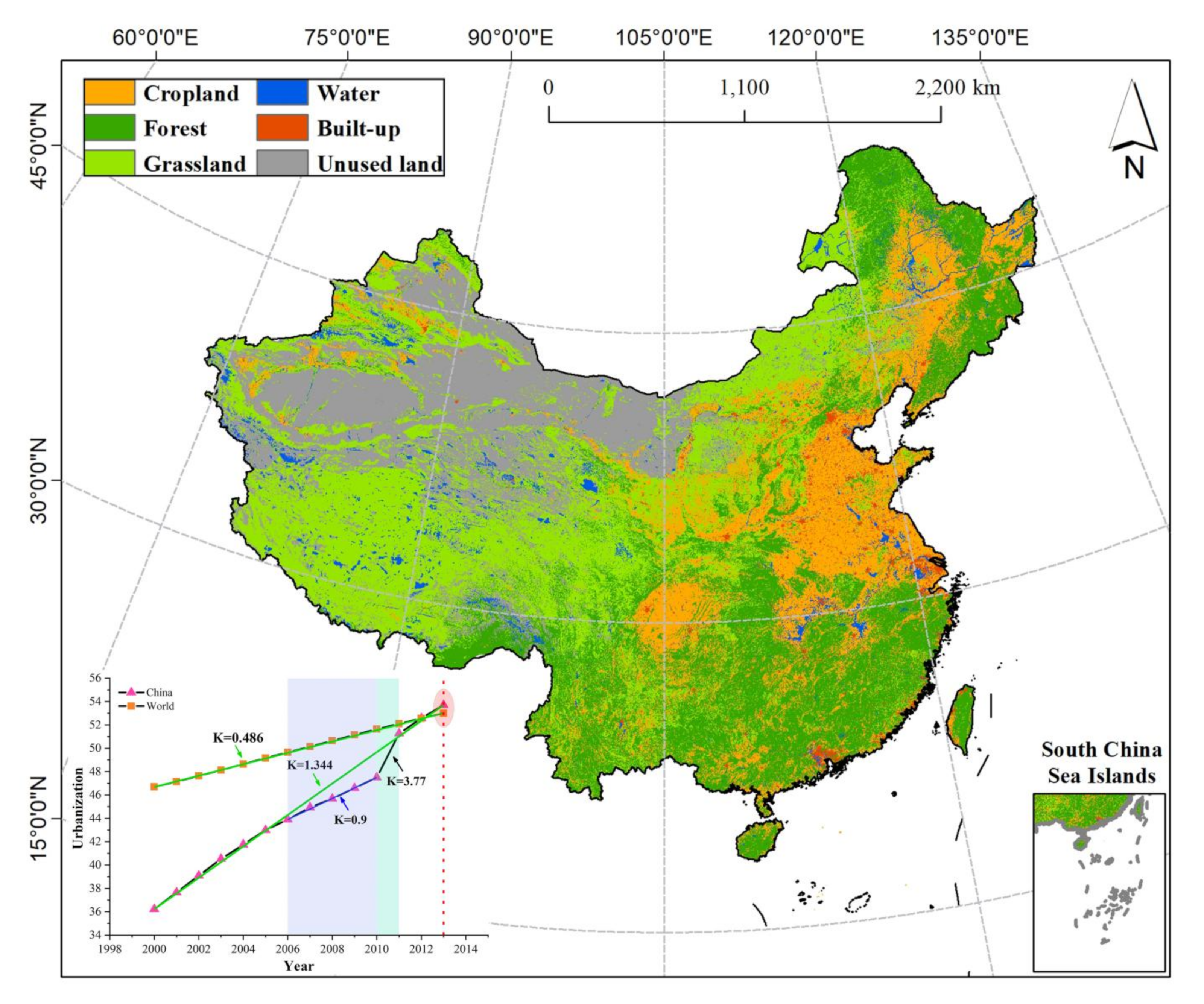
2.1. Study Area
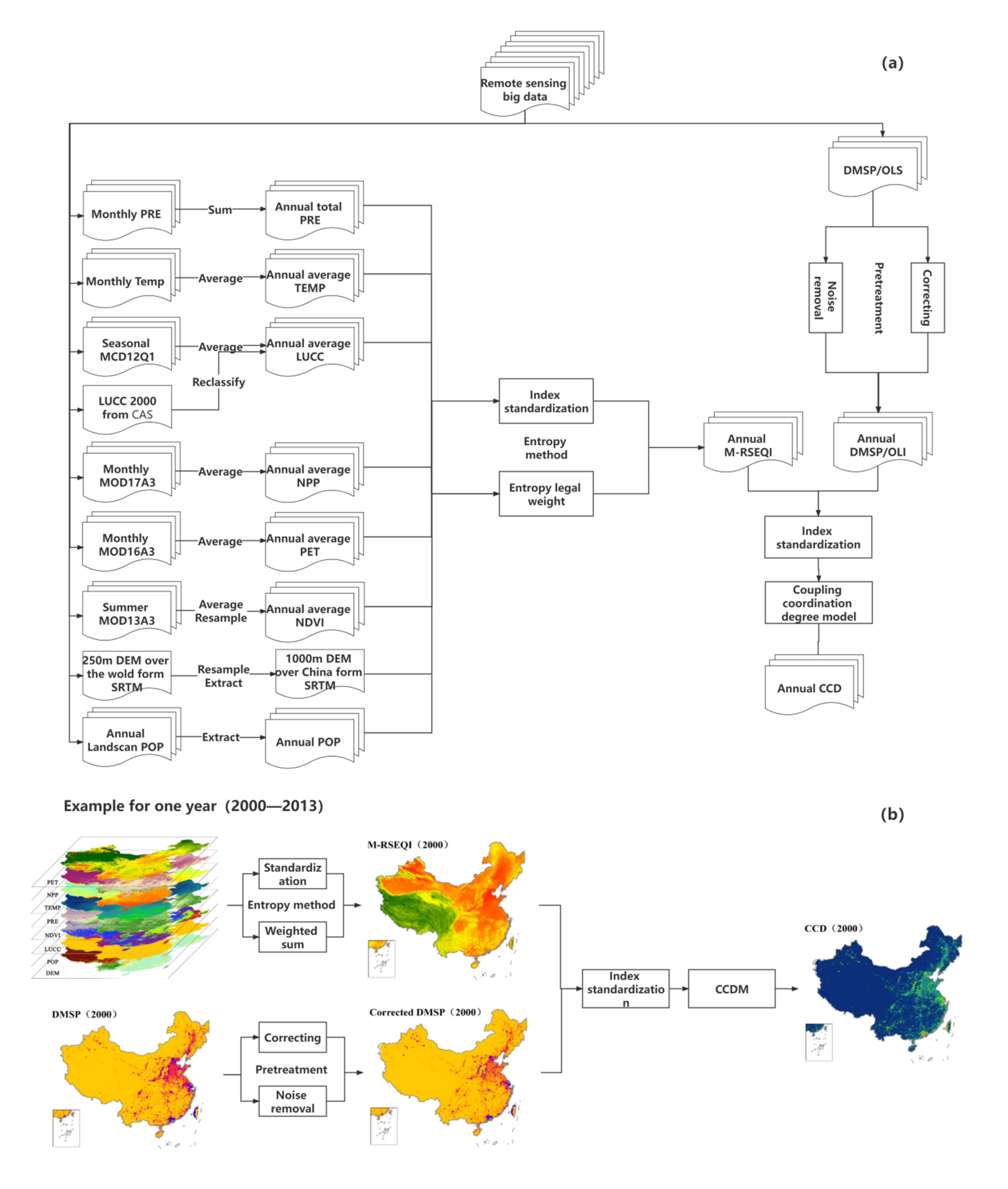
2.2. Data
3. Methods
3.1. M-RSEQI
3.2. Urbanization Assessment Based on DMSP
3.3. Coupling Coordination Degree Model (CCDM)
3.4. Trend Analysis
4. Results
4.1. M-RSEQI
4.1.1. Rationality of M-RSEQI
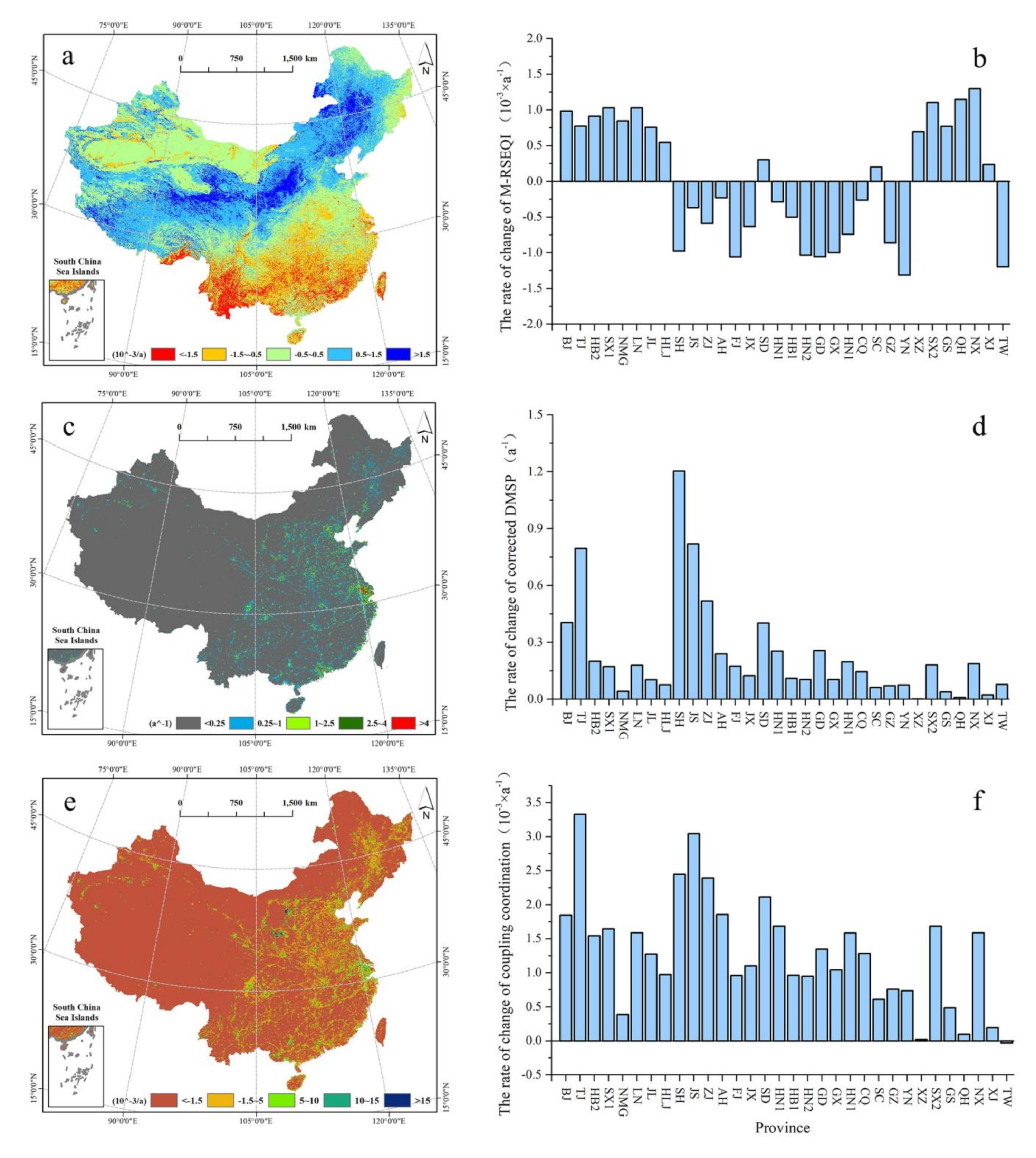
4.1.2. Spatiotemporal Changes in M-RSEQI
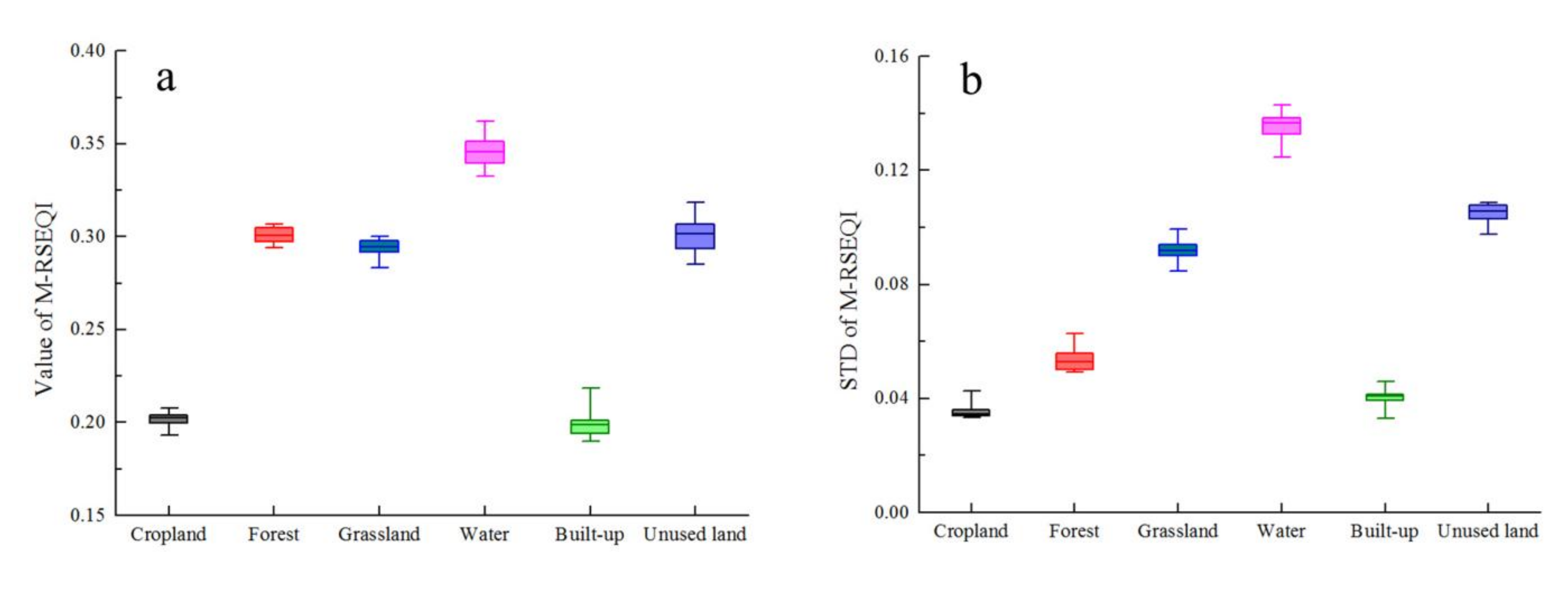
4.1.3. M-RSEQI in Different Ecosystems
4.2. Urbanization
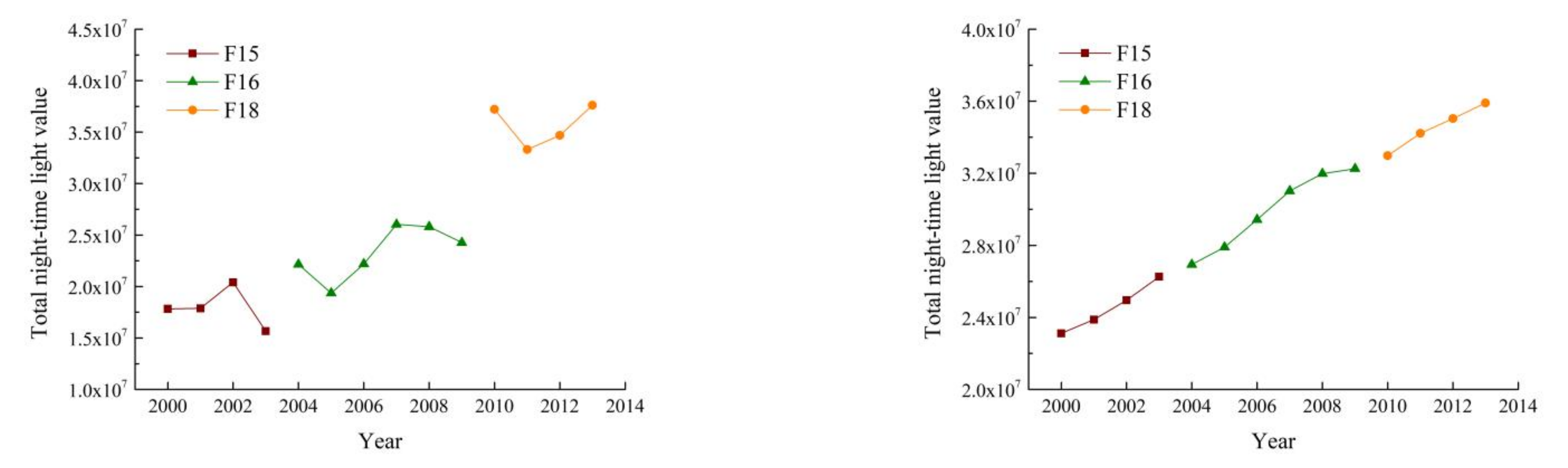
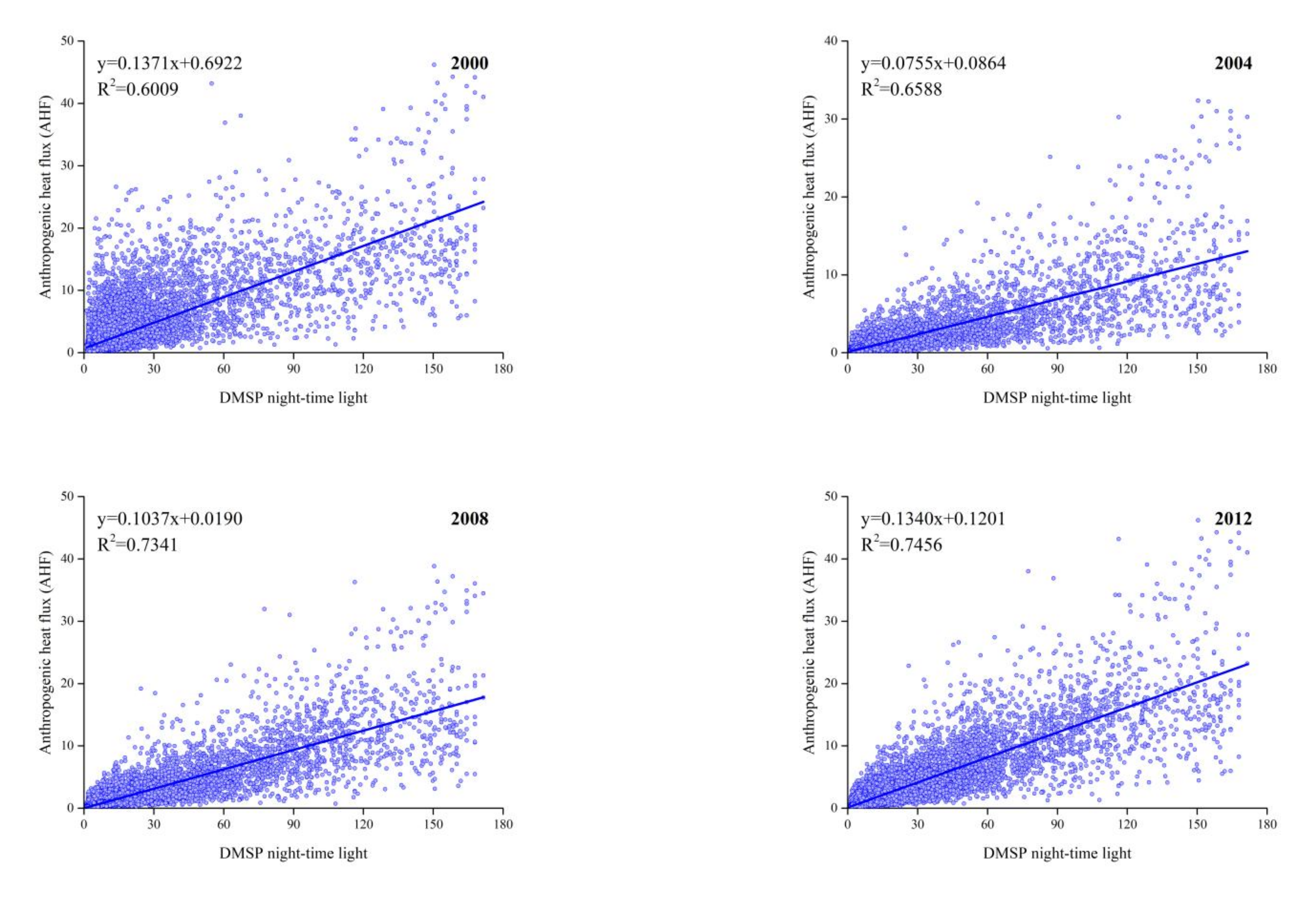
4.2.1. Validity of Corrected DMSP
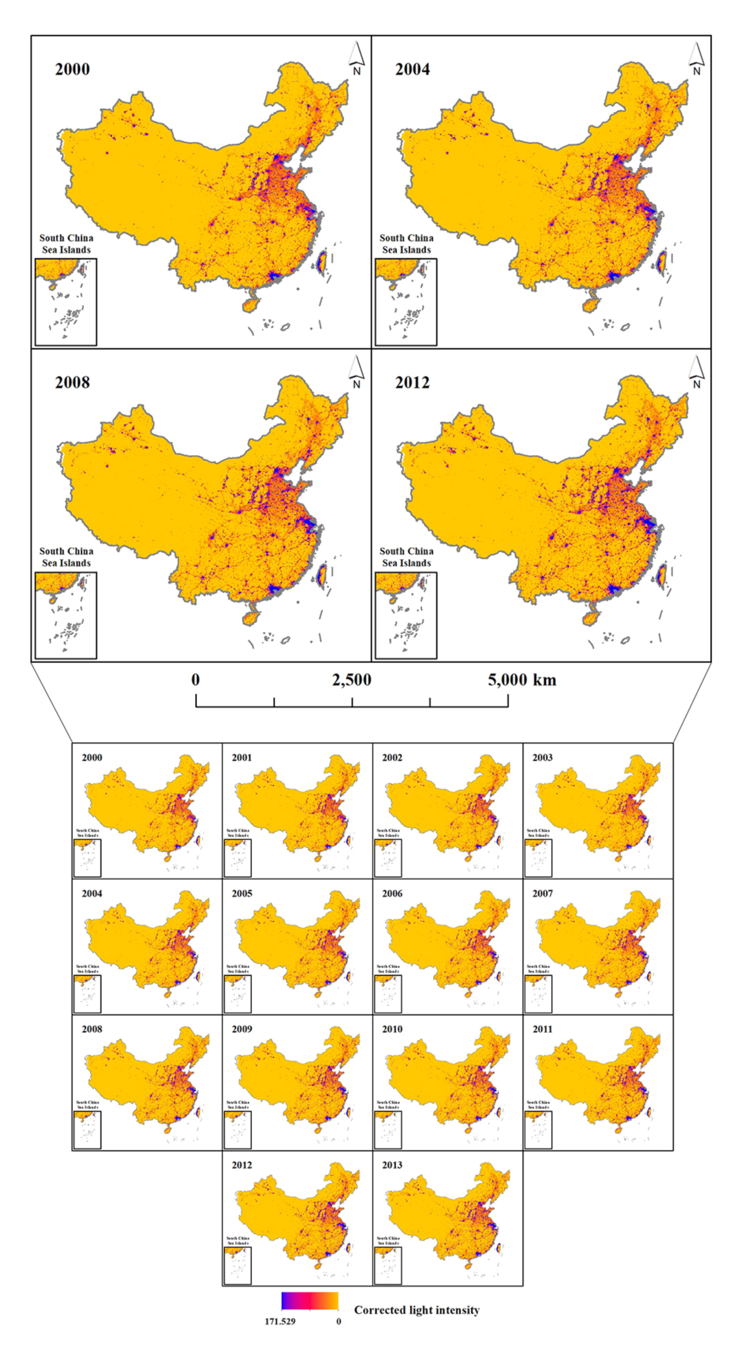
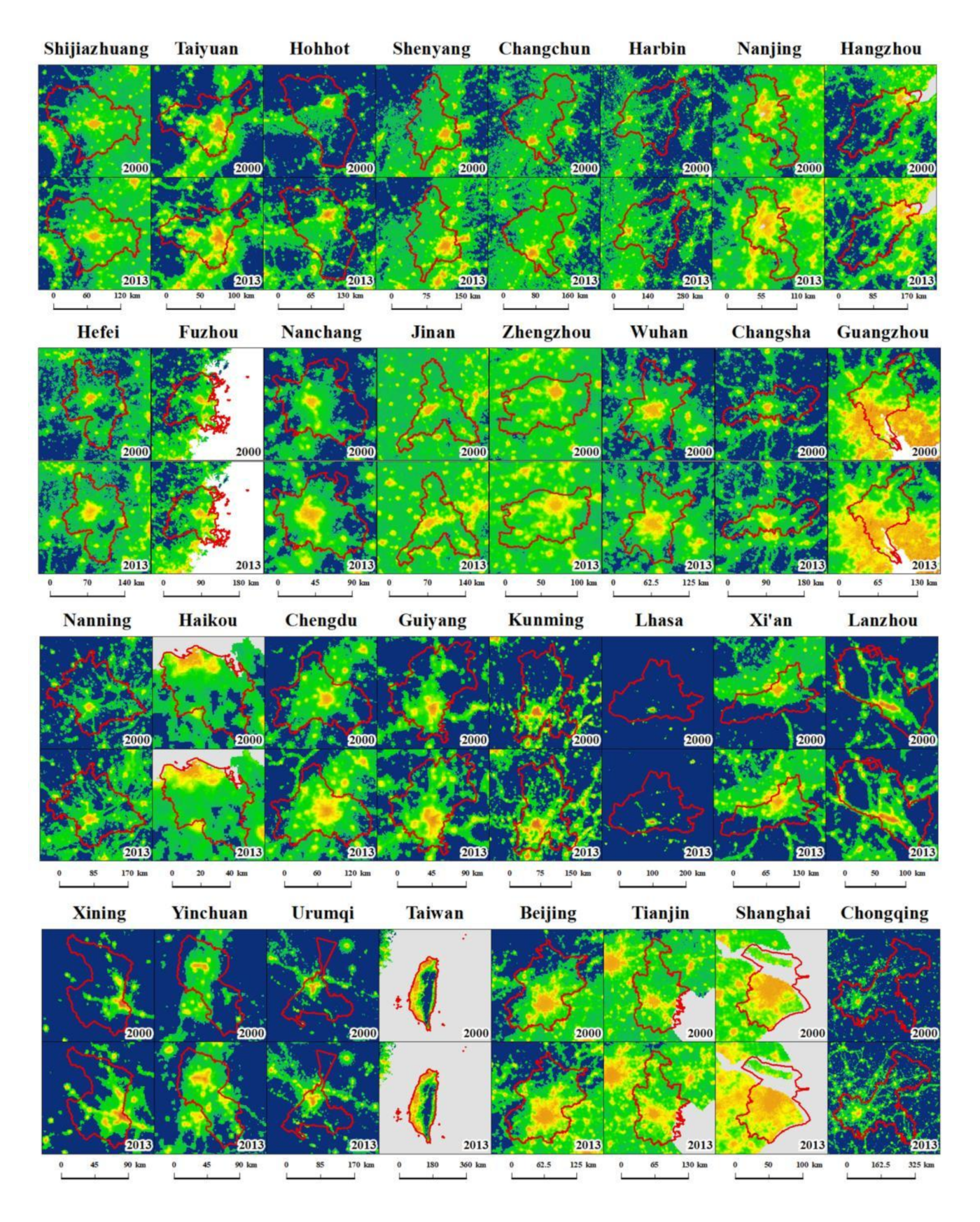
4.2.2. Spatiotemporal Changes in Urbanization
4.3. CCD
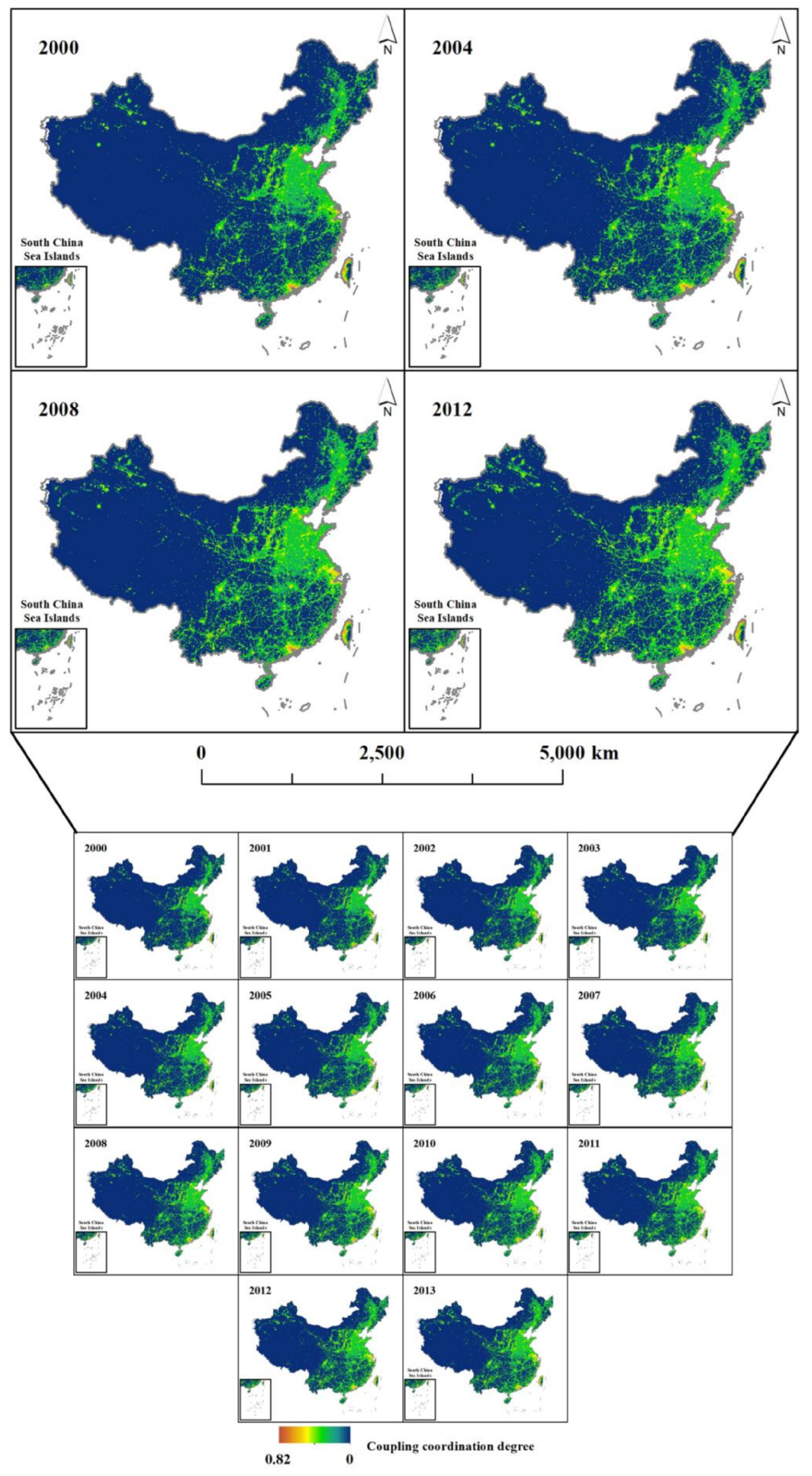
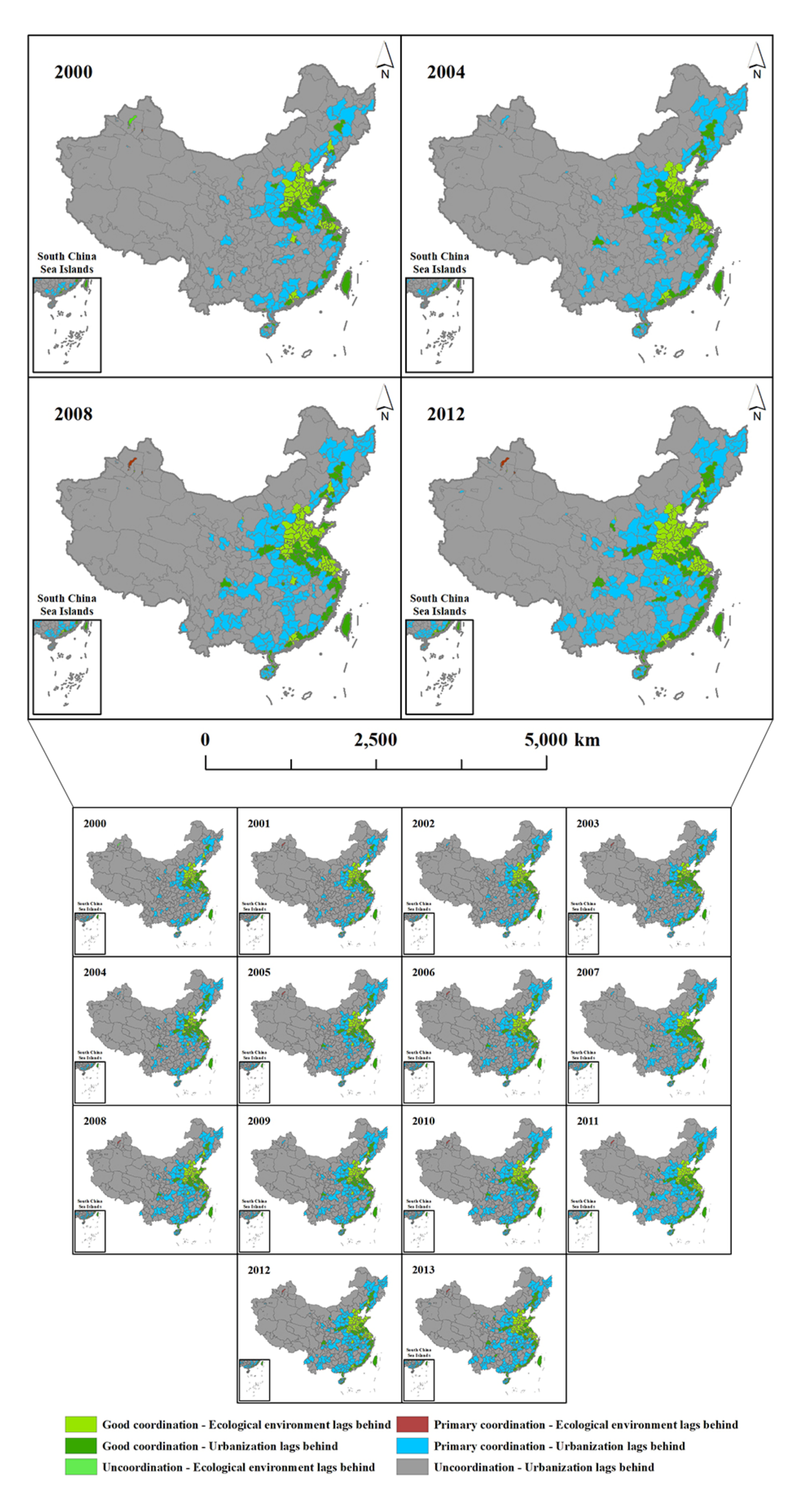
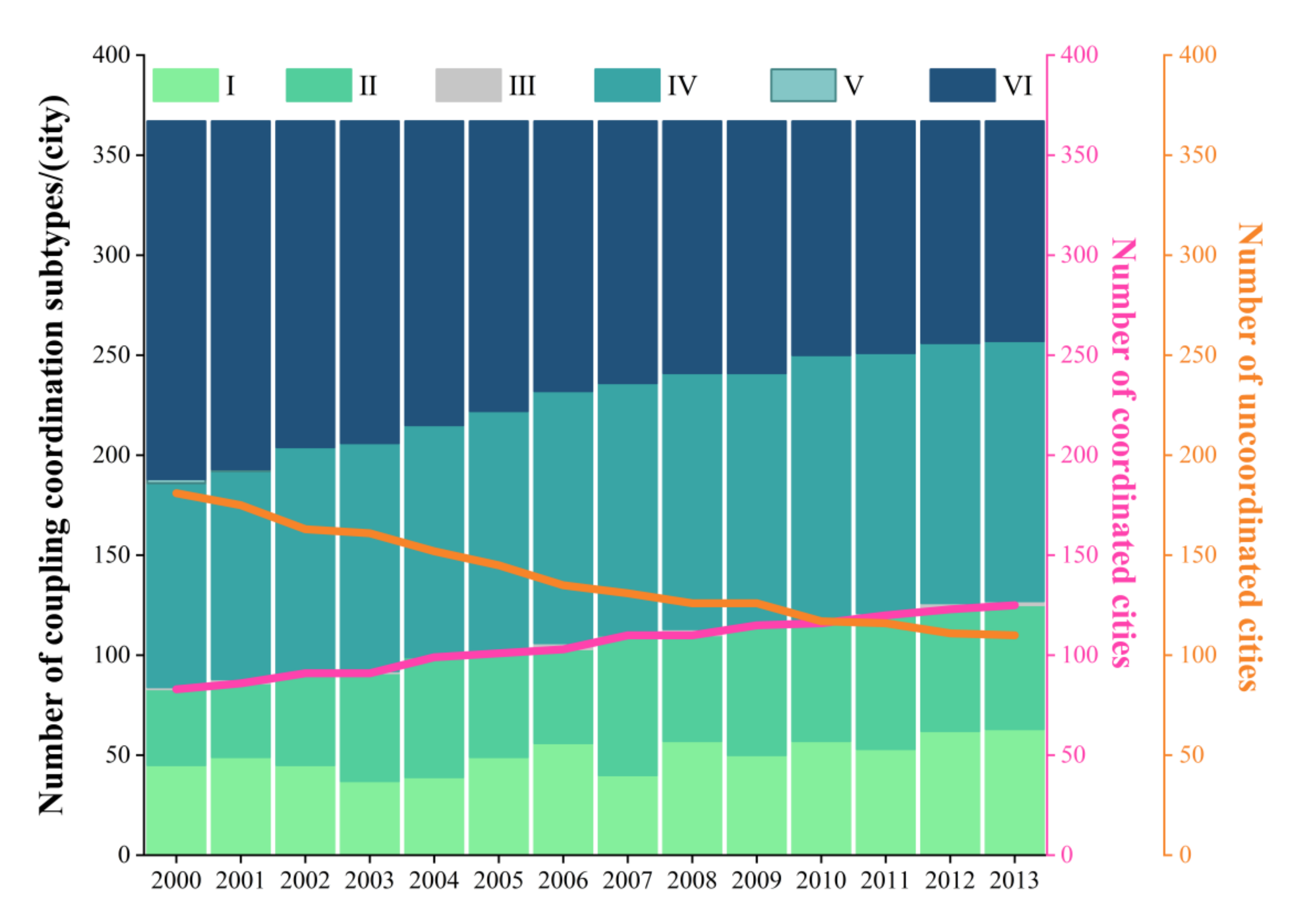
4.3.1. Spatiotemporal Changes in CCD
4.3.2. Change Characteristics of the CCD in Different Ecosystems
5. Discussion
5.1. Coupling Mechanism Analysis
5.2. Limitations and Prospects
6. Conclusions
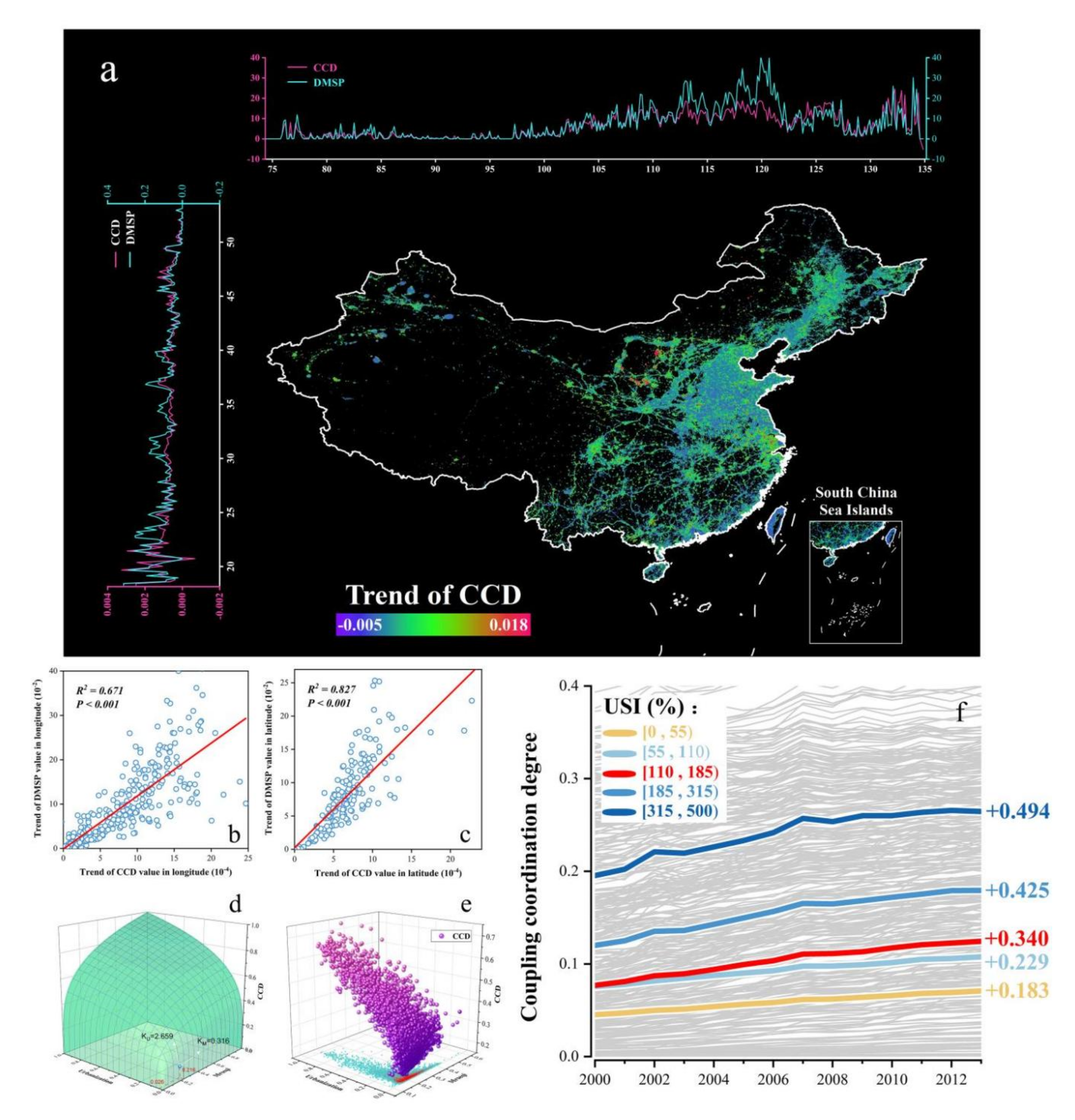
- The decisive factor affecting the CCD was urbanization development in 2013. The impact that the degree of urbanization had on the CCD was approximately 8.4 times higher than that of the EEQ.
- From 2000 to 2013, the urbanization development of China showed the characteristics of “fast in the east and slow in the west” over the course of the past 14 years. The CCD between the EEQ and urbanization in China showed the characteristic of “strong in the east, weak in the west”.
- Most of China’s cities were in an uncoordinated state and were concentrated in the central and western regions of China. The coupling pattern of EEQ and urbanization in China evolved from “uncoordinated cities into coordinated cities, with the characteristic of “urbanization lags behind EEQ” evolving into “EEQ lags behind urbanization”.
Author Contributions
Funding
Institutional Review Board Statement
Informed Consent Statement
Data Availability Statement
Acknowledgments
Conflicts of Interest
References
- Shan, G.; Xianjin, H. Performance Evaluation of Eco-construction Based on PSR Model in China from 1953 to 2008. J. Nat. Resour. 2010, 25, 341–350. [Google Scholar]
- Sun, D.; Zhang, J.; Zhu, C. An Assessment of China’s Ecological Environment Quality Change and Its Spatial Variation. Acta Geogr. Sin. 2012, 67, 1599–1610. [Google Scholar]
- McKinney, M.L. Effects of urbanization on species richness: A review of plants and animals. Urban Ecosyst. 2008, 11, 161–176. [Google Scholar] [CrossRef]
- Xiuxing, Y. An Assessment of China’s Ecological Environment Quality Change and the Spatial Variation. Environ. Life 2014, 9X, 249. [Google Scholar]
- Wei, Y.L.; Bao, L.J.; Wu, C.C.; He, Z. Assessing the effects of urbanization on the environment with soil legacy and current-use insecticides: A case study in the Pearl River Delta, China. Sci. Total Environ. 2015, 514, 409–417. [Google Scholar] [CrossRef]
- Liu, X.; Ma, L.; Li, X.; Ai, B.; Li, S.; He, Z. Simulating urban growth by integrating landscape expansion index (LEI) and cellular automata. Int. J. Geogr. Inf. Sci. 2014, 28, 148–163. [Google Scholar] [CrossRef]
- Zhu, J. The 2030 Agenda for Sustainable Development and China’s implementation. Chin. J. Popul. Resour. Environ. 2016, 15, 142–146. [Google Scholar] [CrossRef]
- Wang, S.-X.; Yao, Y.; Zhou, Y. Analysis of Ecological Quality of the Environment and Influencing Factors in China during 2005–2010. Int. J. Environ. Res. Public Health 2014, 11, 1673–1693. [Google Scholar] [CrossRef]
- Du, W. Research on the Evaluation Index of Air Pollution Control Audit Based on PSR Model; IOP Conference Series: Earth and Environmental Science; IOP Publishing: Bristol, UK, 2020; Volume 514. [Google Scholar]
- McDonald Michael, E. EMAP Overview: Objectives, Approaches, and Achievements; Monitoring Ecological Condition in the Western United States; Springer: Dordrecht, The Netherlands, 2000; pp. 3–8. [Google Scholar]
- Smith, E.R. An Overview of EPA’s Regional Vulnerability Assessment (ReVA) Program. Environ. Monit. Assess. 2000, 64, 9–15. [Google Scholar] [CrossRef]
- US Forest Service. Forest Service Resource Inventories: An Overview. 1992. Available online: https://www.fs.usda.gov/treesearch/pubs/123 (accessed on 23 December 2021).
- Ahmed, Z.; Wang, Z.; Mahmood, F.; Hafeez, M.; Ali, N. Does globalization increase the ecological footprint? Empirical evidence from Malaysia. Environ. Sci. Pollut. Res. 2019, 26, 18565–18582. [Google Scholar] [CrossRef]
- Shah, S.A.A.; Zhou, P.; Walasai, G.; Mohsin, M. Energy security and environmental sustainability index of South Asian countries: A composite index approach. Ecol. Indic. 2019, 106, 105507. [Google Scholar] [CrossRef]
- Xu, C.; Wang, S. A comprehensive quantitative evaluation of new sustainable urbanization level in 20 Chinese urban agglomerations. Sustainability 2016, 8, 91. [Google Scholar] [CrossRef] [Green Version]
- Xu, D.; Hou, G. The Spatiotemporal Coupling Characteristics of Regional Urbanization and Its Influencing Factors: Taking the Yangtze River Delta as an Example. Sustainability 2019, 11, 822. [Google Scholar] [CrossRef] [Green Version]
- Zhang, W.; Wang, M. Spatial-temporal characteristics and determinants of land urbanization quality in China: Evidence from 285 prefecture-level cities. Sustain. Cities Soc. 2018, 38, 70–79. [Google Scholar] [CrossRef]
- Elmqvist, T.; Fragkias, M.; Goodness, J.; Güneralp, B.; Marcotullio, P.J.; McDonald, R.I.; Parnell, S.; Schewenius, M.; Sendstad, M.; Seto, K.C.; et al. Urbanization, Biodiversity and Ecosystem Services: Challenges and Opportunities: A Global Assessment; Springer Nature: Dordrecht, The Netherlands, 2013. [Google Scholar]
- Shao, Z.; Ding, L.; Li, D.; Altan, O.; Huq, E.; Li, C. Exploring the Relationship between Urbanization and Ecological Environment Using Remote Sensing Images and Statistical Data: A Case Study in the Yangtze River Delta, China. Sustainability 2020, 12, 5620. [Google Scholar] [CrossRef]
- Chen, W.; Zhang, Y.; Pengwang, C.; Gao, W. Evaluation of Urbanization Dynamics and its Impacts on Surface Heat Islands: A Case Study of Beijing, China. Remote Sens. 2017, 9, 453. [Google Scholar] [CrossRef] [Green Version]
- Estoque, R.C. A review of the sustainability concept and the state of SDG monitoring using remote sensing. Remote Sens. 2020, 12, 1770. [Google Scholar] [CrossRef]
- Xu, H. Remote Sensing Evaluation Index of Regional Ecological Environment Changes. China Environ. Sci. 2013, 33, 889–897. [Google Scholar]
- Shan, W.; Jin, X.; Ren, J.; Wang, Y.; Xu, Z.; Fan, Y.; Gu, Z.; Hong, C.; Lin, J.; Zhou, Y. Ecological environment quality assessment based on remote sensing data for land consolidation. J. Clean. Prod. 2019, 239, 118126. [Google Scholar] [CrossRef]
- Guo, B.; Yelin, F.; Xiaobin, J. Monitoring the effects of land consolidation on the ecological environmental quality based on remote sensing: A case study of Chaohu Lake Basin, China. Land Use Policy 2020, 95, 104569. [Google Scholar] [CrossRef]
- Xu, H.; Wang, M.; Shi, T.; Guan, H.; Fang, C.; Lin, Z. Prediction of ecological effects of potential population and impervious surface increases using a remote sensing based ecological index (RSEI). Ecol. Indic. 2018, 93, 730–740. [Google Scholar] [CrossRef]
- Liao, W.; Jiang, W. Evaluation of the Spatiotemporal Variations in the EEQ in China Based on the Remote Sensing Ecological Index. Remote Sens. 2020, 12, 2462. [Google Scholar] [CrossRef]
- Li, K.; Chen, Y. A Genetic Algorithm-based urban cluster automatic threshold method by combining VIIRS DNB, NDVI, and NDBI to monitor urbanization. Remote Sens. 2018, 10, 277. [Google Scholar] [CrossRef] [Green Version]
- Zhang, Q.; Seto, K.C. Mapping urbanization dynamics at regional and global scales using multi-temporal DMSP/OLS nighttime light data. Remote Sens. Environ. 2011, 115, 2320–2329. [Google Scholar] [CrossRef]
- Ma, T.; Zhou, Y.; Zhou, C.; Haynie, S.; Pei, T.; Xu, T. Night-time light derived estimation of spatio-temporal characteristics of urbanization dynamics using DMSP/OLS satellite data. Remote Sens. Environ. 2015, 158, 453–464. [Google Scholar] [CrossRef]
- Zheng, Z.; Wu, Z.; Chen, Y.; Yang, Z.; Marinello, F. Exploration of eco-environment and urbanization changes in coastal zones: A case study in China over the past 20 years. Ecol. Indic. 2020, 119, 106847. [Google Scholar] [CrossRef]
- Chen, J.; Zhuo, L.; Shi, P.J. The study on urbanization process in China based on DMSP/OLS data: Development of a light index for urbanization level estimation. J. Remote Sens. 2003, 7, 168–175. [Google Scholar]
- Fang, C.; Wang, S.; Li, G. Changing urban forms and carbon dioxide emissions in China: A case study of 30 provincial capital cities. Appl. Energy 2015, 158, 519–531. [Google Scholar] [CrossRef]
- Ozokcu, S.; Özdemir, O. Economic growth, energy, and environmental Kuznets curve. Renew. Sustain. Energy Rev. 2017, 72, 639–647. [Google Scholar] [CrossRef]
- Fanning Andrew, L.; O’Neill, D.W.; Büchs, M. Provisioning systems for a good life within planetary boundaries. Glob. Environ. Change 2020, 64, 102135. [Google Scholar] [CrossRef]
- O’Neill, D.W.; Fanning, A.L.; Lamb, W.F.; Steinberger, J.K. A good life for all within planetary boundaries. Nat. Sustain. 2018, 1, 88–95. [Google Scholar] [CrossRef] [Green Version]
- Fang, C.; Ren, Y. Analysis of emergy-based metabolic efficiency and environmental pressure on the local coupling and telecoupling between urbanization and the eco-environment in the Beijing-Tianjin-Hebei urban agglomeration. Sci. China Earth Sci. 2017, 60, 1083–1097. [Google Scholar] [CrossRef]
- Andrea, L.; Newig, J.; Challies, E. Globalization’s limits to the environmental state? Integrating telecoupling into global environmental governance. Environ. Politics 2016, 25, 136–159. [Google Scholar]
- Yi, Y.; Meng, G. A bibliometric analysis of comparative research on the evolution of international and Chinese ecological footprint research hotspots and frontiers since 2000. Ecol. Indic. 2019, 102, 650–665. [Google Scholar]
- Rashid, A.; Irum, A.; Malik, I.A.; Ashraf, A.; Rongqiong, L.; Liu, G.; Ullah, H.; Ali, M.U.; Yousaf, B. Ecological footprint of Rawalpindi; Pakistan’s first footprint analysis from urbanization perspective. J. Clean. Prod. 2018, 170, 362–368. [Google Scholar] [CrossRef]
- Beloin-Saint-Pierre, D.; Rugani, B.; Lasvaux, S.; Mailhac, A.; Popovici, E.; Sibiude, G.; Benetto, E.; Schiopu, N. A review of urban metabolism studies to identify key methodological choices for future harmonization and implementation. J. Clean. Prod. 2017, 163, S223–S240. [Google Scholar] [CrossRef]
- Wu, Y.; Que, W.; Liu, Y.-G.; Li, J.; Cao, L.; Liu, S.-B.; Zeng, G.-M.; Zhang, J. Efficiency estimation of urban metabolism via Emergy, DEA of time-series. Ecol. Indic. 2018, 85, 276–284. [Google Scholar] [CrossRef]
- Yang, S.; Cao, D.; Lo, K. Analyzing and optimizing the impact of economic restructuring on Shanghai’s carbon emissions using STIRPAT and NSGA-II. Sustain. Cities Soc. 2018, 40, 44–53. [Google Scholar] [CrossRef]
- Song, Q.; Zhou, N.; Liu, T.; Siehr, S.A.; Qi, Y. Investigation of a “coupling model” of coordination between low-carbon development and urbanization in China. Energy Policy 2018, 121, 346–354. [Google Scholar] [CrossRef] [Green Version]
- Lowe, R.; Wu, Y.; Tamar, A.; Harb, J.; Abbeel, P.; Mordatch, I. Multi-agent actor-critic for mixed cooperative-competitive environments. Advances in neural information processing systems. arXiv 2017, arXiv:1706.02275. [Google Scholar]
- Fang, C.; Liu, H.; Li, G. International progress and evaluation on interactive coupling effects between urbanization and the eco-environment. J. Geogr. Sci. 2016, 26, 1081–1116. [Google Scholar] [CrossRef]
- Zhao, Y.; Wang, S.; Zhou, C. Understanding the relation between urbanization and the eco-environment in China’s Yangtze River Delta using an improved EKC model and coupling analysis. Sci. Total Environ. 2016, 571, 862–875. [Google Scholar] [CrossRef] [PubMed]
- Li, Y.; Li, Y.; Zhou, Y.; Shi, Y.; Zhu, X. Investigation of a coupling model of coordination between urbanization and the environment. J. Environ. Manag. 2012, 98, 127–133. [Google Scholar] [CrossRef] [PubMed]
- Wang, S.J.; Ma, H.; Zhao, Y.B. Exploring the relationship between urbanization and the eco-environment—A case study of Beijing–Tianjin–Hebei region. Ecol. Indic. 2014, 45, 171–183. [Google Scholar] [CrossRef]
- Li, W.; Yi, P. Assessment of city sustainability—Coupling coordinated development among economy, society and environment. J. Clean. Prod. 2020, 256, 120453. [Google Scholar] [CrossRef]
- Qu, B.; Zhang, Y.; Kang, S.; Sillanpää, M. Water quality in the Tibetan Plateau: Major ions and trace elements in rivers of the “Water Tower of Asia”. Sci. Total Environ. 2019, 649, 571–581. [Google Scholar] [CrossRef]
- Fan, Y.; Fang, C.; Zhang, Q. Coupling coordinated development between social economy and ecological environment in Chinese provincial capital cities-assessment and policy implications. J. Clean. Prod. 2019, 229, 289–298. [Google Scholar] [CrossRef]
- Peng, S.; Ding, Y.; Liu, W.; Li, Z. 1 km monthly temperature and precipitation dataset for China from 1901 to 2017. Earth Syst. Sci. Data 2019, 11, 1931–1946. [Google Scholar] [CrossRef] [Green Version]
- Wang, S.; Hu, D.; Yu, C.; Chen, S.; Di, Y. Mapping China’s time-series anthropogenic heat flux with inventory method and multi-source remotely sensed data. Sci. Total Environ. 2020, 734, 139457. [Google Scholar] [CrossRef]
- Zhao, G.; Chen, L.; Mu, J. Discussion on Construction of Ecological Environment Quality Evaluation System. Meteorol. Environ. Sci. 2018, 2018, 1–11. [Google Scholar]
- Lu, Y.; Xiang, P. Analysis of the Coupling Relationship between Ecological Environment and Urbanization:Chang-Zhu-Tan Urban Agglomeration in Hunan Province, China as a Case. Urban Dev. Res. 2020, 1, 19. [Google Scholar]
- Cao, Z.; Wu, Z.; Kuang, Y.; Huang, N. Correction of DMSP/OLS Night-time Light Images and Its Application in China. J. Earth Inf. Sci. 2015, 17, 1092–1102. [Google Scholar]
- Cao, Z.; Wu, Z.; Mi, S.; Yang, K. A Method for Classified Correction of Stable DMSP/OLS night-time Light Imagery across China. J. Earth Inf. Sci. 2020, 22, 246–257. [Google Scholar]
- Liao, L.; Dai, W.; Huang, F.H.; Hu, Q. Coupling Coordination Analysis of Urbanization and Eco-environment System in Jinjiang Using Landsat Series Data and DMSP/OLS Nighttime Light Data. J. Fujian Norm. Univ. Nat. Sci. Ed. 2018, 6, 16. [Google Scholar]
- Yajie, Z.; Huizhi, L. Spatial-Temporal Coupled Coordination between Urbanization and Ecological Environment in Yangtze River Economic Belt. Bull. Soil Water Conserv. 2018, 37, 334–340. [Google Scholar]
- Li, S.; Yan, J.; Wan, J. The Spatial-temporal Changes of Vegetation Restoration on Loess Plateau in Shaanxi-Gansu-Ningxia Region. Acta Geogr. Sin. 2012, 67, 960–970. [Google Scholar]
- Chen, J.; Jia, W.; Zhao, Z.; Zhang, Y.; Liu, Y. Research on Temporal and Spatial Variation Characteristics of Vegetation Cover of Qilian Mountains from 1982 to 2006. Adv. Earth Sci. 2015, 30, 834–845. [Google Scholar]
- Fensholt, R.; Proud, S.R. Evaluation of earth observation based global long term vegetation trends—Comparing GIMMS and MODIS global NDVI time series. Remote Sens. Environ. 2012, 119, 131–147. [Google Scholar] [CrossRef]
- Yuan, S.; Huichun, S.; Minhui, X.; Pengxia, Z. Spatiotemporal evolution pattern and influencing factors of EEQ in Gansu from 2000 to 2017. J. Ecol. 2019, 38, 3800–3808. [Google Scholar]
- Zhou, Z.; Wang, X.; Ding, Z.; Chen, Y.; Wang, C. Remote sensing analysis of ecological quality change in Xinjiang. J. Ecol. 2020, 40, 2907–2919. [Google Scholar]
- Xu, D.; Yang, F.; Yu, L.; Zhou, Y.; Li, H.; Ma, J.; Huang, J.; Wei, J.; Xu, Y.; Zhang, C.; et al. Quantization of the coupling mechanism between eco-environmental quality and urbanization from multisource remote sensing data. J. Clean. Prod. 2021, 321, 128948. [Google Scholar] [CrossRef]
- Dewan, A.M.; Yamaguchi, Y. Land use and land cover change in Greater Dhaka, Bangladesh: Using remote sensing to promote sustainable urbanization. Appl. Geogr. 2009, 29, 390–401. [Google Scholar] [CrossRef]
- Taubenböck, H.; Wegmann, M.; Roth, A.; Mehl, H.; Dech, S. Urbanization in India–Spatiotemporal analysis using remote sensing data [J]. Comput. Environ. Urban Syst. 2009, 33, 179–188. [Google Scholar] [CrossRef]
- Xu, Y.; Yu, L.; Peng, D.; Zhao, J.; Cheng, Y.; Liu, X.; Li, W.; Meng, R.; Xu, X.; Gong, P. Annual 30-m land use/land cover maps of China for 1980–2015 from the integration of AVHRR, MODIS and Landsat data using the BFAST algorithm. Sci. China Earth Sci. 2020, 63, 1390–1407. [Google Scholar] [CrossRef]
- Kyba, C.; Kuester, T.; de Miguel, A.S.; Baugh, K.; Jechow, A.; Hölker, F.; Bennie, J.; Elvidge, C.; Gaston, K.; Guanter, L. Artificially lit surface of Earth at night increasing in radiance and extent. Sci. Adv. 2017, 3, e1701528. [Google Scholar] [CrossRef] [Green Version]


| Data Name | Format | Spatial Resolution | Time Resolution | Source |
|---|---|---|---|---|
| 2019QZKK0603-zgyjsl [52] | NETCDF | 1000 m | Monthly | NTPDC a |
| 2019QZKK0603-zgypjw [52] | NETCDF | 1000 m | Monthly | NTPDC a |
| MOD17A3 | HDF | 1000 m | Monthly | NASA b |
| MOD13A3 | HDF | 250 m | Monthly | NASA b |
| SRTM DEM | TIFF | 250 m | — | USGS c |
| MCD12Q1 | HDF | 1000 m | Seasonal | NASA b |
| Landscan POP | TIFF | 1000 m | Annual | ORNL d |
| MOD16A3 | HDF | 1000 m | Monthly | NASA b |
| LUCC2000 | TIFF | 1000 m | Annual | CAS e |
| DMSP nighttime light | TIFF | 1000 m | Annual | NOAA f |
| Anthropogenic heat flux (AHF) | TIFF | 1000 m | Annual | Article [53] |
| CCD | Progression Stage | Comparison | Subcategories |
|---|---|---|---|
| 0 ≤ D < 0.2 | Uncoordinated | U < E | Urbanization lags behind |
| U > E | Eco-environment lags behind | ||
| 0.2 ≤ D < 0.4 | Primary coordinated | U < E | Urbanization lags behind |
| U > E | Eco-environment lags behind | ||
| 0.4 ≤ D ≤ 1 | Coordinated | U < E | Urbanization lags behind |
| U > E | Eco-environment lags behind |
| Indicator | VIF | TOL |
|---|---|---|
| PRE | 8.097 | 0.123 |
| TEMP | 9.411 | 0.106 |
| NPP | 5.758 | 0.174 |
| NDVI | 5.922 | 0.169 |
| DEM | 2.975 | 0.336 |
| LUCC | 4.095 | 0.244 |
| POP | 1.349 | 0.741 |
| PET | 2.634 | 0.380 |
Publisher’s Note: MDPI stays neutral with regard to jurisdictional claims in published maps and institutional affiliations. |
© 2022 by the authors. Licensee MDPI, Basel, Switzerland. This article is an open access article distributed under the terms and conditions of the Creative Commons Attribution (CC BY) license (https://creativecommons.org/licenses/by/4.0/).
Share and Cite
Xu, D.; Cheng, J.; Xu, S.; Geng, J.; Yang, F.; Fang, H.; Xu, J.; Wang, S.; Wang, Y.; Huang, J.; et al. Understanding the Relationship between China’s Eco-Environmental Quality and Urbanization Using Multisource Remote Sensing Data. Remote Sens. 2022, 14, 198. https://doi.org/10.3390/rs14010198
Xu D, Cheng J, Xu S, Geng J, Yang F, Fang H, Xu J, Wang S, Wang Y, Huang J, et al. Understanding the Relationship between China’s Eco-Environmental Quality and Urbanization Using Multisource Remote Sensing Data. Remote Sensing. 2022; 14(1):198. https://doi.org/10.3390/rs14010198
Chicago/Turabian StyleXu, Dong, Jie Cheng, Shen Xu, Jing Geng, Feng Yang, He Fang, Jinfeng Xu, Sheng Wang, Yubai Wang, Jincai Huang, and et al. 2022. "Understanding the Relationship between China’s Eco-Environmental Quality and Urbanization Using Multisource Remote Sensing Data" Remote Sensing 14, no. 1: 198. https://doi.org/10.3390/rs14010198