
Integrating SAR and Optical Remote Sensing for Conservation-Targeted Wetlands Mapping


1
Marine Science Institute, The University of Texas at Austin, Port Aransas, TX 78373, USA
2
Ducks Unlimited Inc., Bismarck, ND 58503, USA
*
Author to whom correspondence should be addressed.
Remote Sens. 2022, 14(1), 159; https://doi.org/10.3390/rs14010159
Submission received: 12 December 2021
/
Revised: 28 December 2021
/
Accepted: 28 December 2021
/
Published: 30 December 2021
(This article belongs to the Topic Water Management in the Era of Climatic Change)
Abstract
:The Prairie Pothole Region (PPR) contains numerous depressional wetlands known as potholes that provide habitats for waterfowl and other wetland-dependent species. Mapping these wetlands is essential for identifying viable waterfowl habitat and conservation planning scenarios, yet it is a challenging task due to the small size of the potholes, and the presence of emergent vegetation. This study develops an open-source process within the Google Earth Engine platform for mapping the spatial distribution of wetlands through the integration of Sentinel-1 C-band SAR (synthetic aperture radar) data with high-resolution (10-m) Sentinel-2 bands. We used two machine-learning algorithms (random forest (RF) and support vector machine (SVM)) to identify wetlands across the study area through supervised classification of the multisensor composite. We trained the algorithms with ground truth data provided through field studies and aerial photography. The accuracy was assessed by comparing the predicted and actual wetland and non-wetland classes using statistical coefficients (overall accuracy, Kappa, sensitivity, and specificity). For this purpose, we used four different out-of-sample test subsets, including the same year, next year, small vegetated, and small non-vegetated test sets to evaluate the methods on different spatial and temporal scales. The results were also compared to Landsat-derived JRC surface water products, and the Sentinel-2-derived normalized difference water index (NDWI). The wetlands derived from the RF model (overall accuracy 0.76 to 0.95) yielded favorable results, and outperformed the SVM, NDWI, and JRC products in all four testing subsets. To provide a further characterization of the potholes, the water bodies were stratified based on the presence of emergent vegetation using Sentinel-2-derived NDVI, and, after excluding permanent water bodies, using the JRC surface water product. The algorithm presented in the study is scalable and can be adopted for identifying wetlands in other regions of the world.
1. Introduction
Wetlands have been identified as valuable resources that provide a variety of ecological and socioeconomic benefits [1], but they are also threatened due to human activities, such as agricultural intensification and climate change [2]. These threats and others make monitoring the spatiotemporal variation of wetlands’ hydrological processes crucial to their effective management. Here, by hydrological processes, we refer to wetlands’ highly variable environments characterized by hydric soils temporarily or permanently flooded by water. When dry, wetlands resemble surrounding uplands, whereas when inundated, they can have either moist soils or surface water that ranges from centimeters to meters deep. There are also high levels of diversity in wetland cover classes, wherein some inundated wetlands are filled with emergent or submerged vegetation, and others are absent of all vegetation.
Though the dynamic nature of wetlands makes them ecologically valuable to numerous flora and fauna, this also makes them difficult to monitor [3,4]. Monitoring depressional wetlands can also be challenging because these highly dynamic systems are primarily dependent on climate and local weather systems for ponding, and can often be relatively small (<40 ha) [5,6]. The interplay among water, vegetation, and soil results in wetlands that share spectral reflectance characteristics of both aquatic and terrestrial environments. Accurate and unbiased estimates of wetland surface water across the range of natural conditions have therefore eluded scientists.
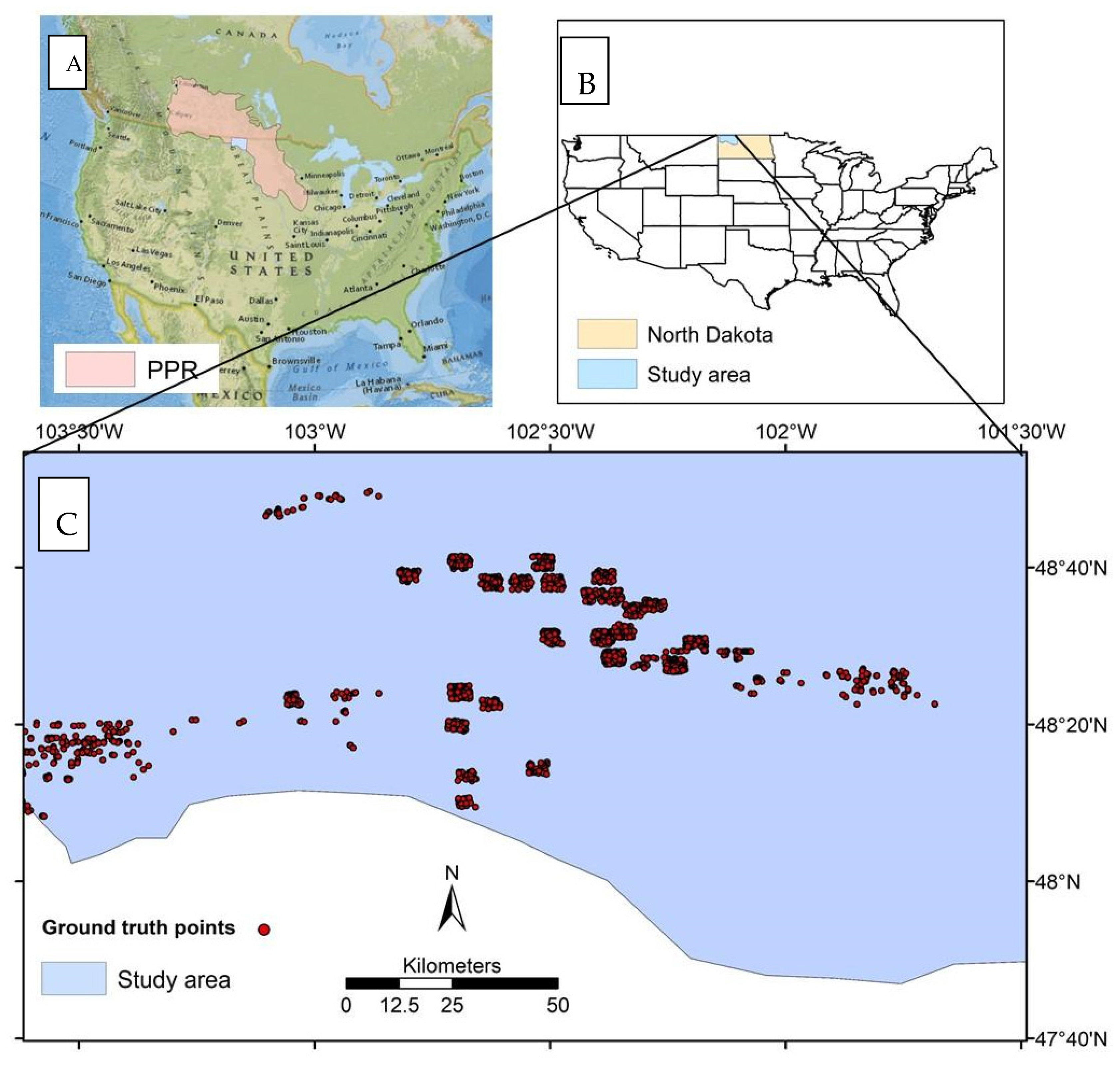
The Prairie Pothole Region (PPR) is one example of a high-risk, dynamic wetland system composed of millions of temporary, seasonal, and semi-permanent depressional wetlands, called potholes. These potholes are known for their cycles of drought and deluge, which drive important ecosystem functions, such as the abundance of aquatic invertebrates [5]. The PPR covers an extensive area of approximately 750,000 km2, including parts of five US states and three Canadian provinces (Figure 1), and provides habitat for over 50% of North America’s migratory waterfowl [7,8]. Hydroperiods in the potholes vary from days to years, but seasonal wetlands that maintain water for less than four months are common [9,10]. Reduced surface water area and changes in hydrology are common in PPR wetlands, for example, as caused by tile draining to allow for higher agricultural production [11], or upland sediment erosion into wetlands, which, though a natural process, is often accelerated by agricultural activity, which fills potholes, and reduces their volume [12]. The total wetland loss in the PPR caused by climate change and human activity was estimated to be 30,000 ha between 1997 and 2009 [10]. A resulting shift towards smaller wetlands and shortened hydroperiods [13,14,15] has underscored a need to understand how these altered hydrological conditions affect ecosystem services and habitat provisioning at broad spatial scales, which starts with an accurate and repeatable estimate of spatial variation in wetland surface water.
Remote sensing analysis can provide broad-scale spatial and temporal information about wetland surface water [16,17]. Previous studies utilized various remote sensing technologies to monitor wetlands across the PPR [8,18]. For example, [8] used high-resolution NAIP data and LIDAR Digital Elevation Models (DEMs) to map PPR wetland inundation, and tested the results with the Wildlife Service National Wetlands Inventory (NWI). However, though NAIP and DEMs can provide fine spatial resolution data (<1 m), these methods cannot capture temporal variation within a season, as NAIP and LiDAR data are not collected intraannually. Optical sensors, such as Sentinel-2 and Landsat, can detect surface water, and have often been used with success for deep, permanent, large water bodies [19,20]. For example, the Joint Research Centre (JRC) provided Landsat-derived surface water products useful for capturing large wetlands. However, the JRC and other products that rely on moderate resolution spectral data often underperform in detecting water in small potholes with dense vegetation canopies and mixed pixels. Others have used Sentinel-1 synthetic aperture radar (SAR) data (spatial resolution: 10 m) to map water extent in the PPR with reasonable success [21,22], as SAR data is robust to cloud cover, and 10 m data provide reasonable spatial resolution. However, no study has solved all of the challenges for mapping the spatial and temporal variation of surface water in the PPR, and made their algorithm available for long-term monitoring by the research and conservation community. There is a need for open-science algorithms that capture the variation of surface water, can map water even below emergent vegetation, and still represent surface water in smaller potholes.
This study relies on geospatial informatics, which is an expanding field, and includes remote sensing of landscape-scale big data, the development of machine learning tools, and integration with High-Performance Computational (HPC) cloud computing resources. Geospatial informatics offers a unique opportunity for the fast processing of broad-scale remote sensing data in a short time, providing a more comprehensive set of applications, and addressing the limitation of traditional methods [23,24]. The Google Earth Engine (GEE) cloud geospatial computing platform provides a web-based interface to fast parallel processing on Google HPCs with planetary-scale analysis capabilities. The GEE provides a multi-petabyte catalog of global satellite and geospatial datasets [25], such as Landsat, MODIS, and Sentinels. It also gives users the ability to analyze, manipulate, and map the results, and create web-based applications to repeat the analysis [26]. As part of our work, we utilized the capabilities of GEE to create an open-source algorithm for mapping wetlands that can readily be shared with conservation managers and the science community for continued use and development.
To help solve the historical problems of surface water mapping in the PPR, this paper presents a multi-sensor fusion approach that integrates selected fine-resolution (10-m) bands of Sentinel-2 with 10-m Sentinel-1 SAR data, allowing an estimate of both large and small inundated areas. The integration of SAR with optical data also offers complementary information, and can significantly improve the interpretation and classification of results [27,28], for example, by allowing surface water estimates beneath closed-canopy herbaceous vegetation. Altogether, this study aims to provide scalable surface water estimates that can assist with habitat models for wetland-dependent organisms, such as waterbirds or aquatic invertebrates. We will provide our algorithm in a format that can be freely shared and readily implemented by those with minimal coding and modeling experience, such as conservation managers. We achieved this through the following objectives: (1) we developed an open-source framework to map the spatial variation in wetland surface inundation and vegetation based on Sentinel-1 SAR data and Sentinel-2 high-resolution bands within the GEE platform; (2) we deployed this algorithm over a portion of PPR in the high priority conservation area of the PPR; (3) we analyzed the accuracy of this algorithm for generating the information needed for setting conservation targets.
2. Study Area
Our study area was a portion of PPR in North Dakota, USA (Figure 1). The area is dominated by natural grasslands, agricultural areas, and a relatively high density of potholes, which, in this area, often present as small and elliptical water bodies. These numerous small wetlands provide natural habitats for wetland-dependent animals and plant species. We selected this area due to the high density of small potholes, high conservation priority, and availability of ground truth data. We mainly focused our algorithm on a subset of the PPR identified as a high priority conservation site for waterfowl by the United States Fish and Wildlife Service.
3. Data
The data includes a set of aerial imagery to serve as ground truth data, the high-resolution bands (bands 2, 3, 4, and 8) of Sentinel-2, and C-band SAR data Sentinel-1 sensor. We describe the details of the dataset below.
3.1. Ground Truth
Researchers from Duck Unlimited Inc., a non-profit conservation organization, provided the ground truth data. These data include georeferenced aerial photographs of the PPR wetlands in North Dakota collected through a partnership with the United States Fish and Wildlife Service (USFWS). The USFWS used a fixed-wing aircraft to collect imagery in a 1.5 m spatial resolution. If necessary, the images were orthorectified by technicians or research scientists, and used to estimate wet areas during spring and summer for the research projects. We used the summer data of two years (2016 and 2017). These datasets were provided in shapefile formats, and showed wetland boundaries, delineating dry and inundated wetland areas. Some of these wetlands also contained emergent vegetation cover, as identified by field observers (range: 0–80% vegetation cover).
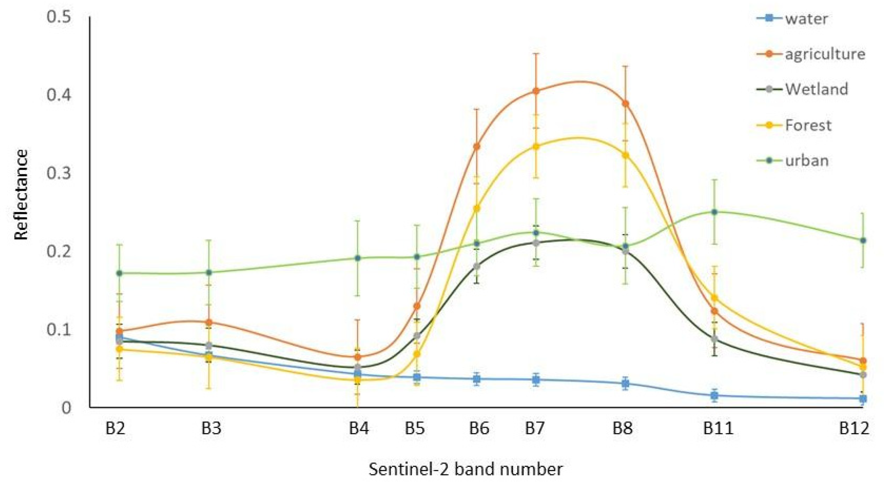
We examined the spectral reflectance of wetland and non-wetland classes, which differed substantially, as indicated by a plot generated for a portion of the study area (Figure 2). The spectral characteristics of wetlands and open water especially differ due to mixed pixels, differences in water depth, the potential presence of vegetation, and variation in water turbidity. Compared to forest and agriculture, deep open water exhibited lower spectral reflectance, as water rapidly absorbs electromagnetic radiation, especially longer wavelengths, and attenuation increases with water depth. The spectral reflectance of wetlands is intermediate to upland vegetation and open water, making wetlands a distinct and highly variable land cover type. Wetlands and moist soils show a dampened near-infrared (NIR) and shortwave infrared (SWIR) reflectance compared with upland vegetation, but are too shallow to attenuate all electromagnetic radiation, as often occurs in deep open water. The spectral characteristics of wetlands will also change rapidly with inundation and vegetation status. To account for this in our ground truth point selection, we selected random points within the digitized wetland surface water area polygon shapefiles to provide the ground truth pixels in GEE. We also included non-wetland training data that represented agriculture, forest, and urban areas. We collected those points using visual observation of high-resolution Google Earth images. The total number of points (including wetland and non-wetland classes) for the years 2016 and 2017 were 895 and 2231, respectively.
Additionally, we provided two out-of-sample subsets for small-vegetated (1440 points) and non-vegetated wetlands (1680 points). Ducks Unlimited provided the vegetation data within the surface water polygons. We used those additional points in a separate accuracy assessment process to evaluate the performance of our method for the smallest wetlands, which are the most challenging to classify as they contain the highest proportion of mixed pixels. The average time difference between ground truth data (wetlands and non-wetlands) and satellite data acquisition was one month.
3.2. Sentinel-1
Sentinel-1 obtains C-band synthetic aperture radar (SAR) images at various polarizations and resolutions. C-band Level-1 Ground Range Detected (GRD) data were obtained through GEE. These data were collected in the Interferometric Wide (IW) swath mode with a spatial resolution of 10 m, a swath width of 250 km, and a repeat cycle of 12 days. These data are available in GEE as preprocessed datasets that express each pixel’s backscatter coefficient (σ°) in decibels (dB). The preprocessing steps include applying orbit files, thermal noise removal, radiometric calibration, and orthorectification (terrain correction). This study used two polarization modes: single co-polarization with vertical transmits and receive (VV), and dual-band co-polarization with vertical transmit and horizontal receive (VH). A total of 20 ascending orbit Sentinel-1 SAR scenes spanning two months were collected over the study area. We used median values of the S1 temporal time series in the multisensory band composite. A median composite can provide a cleaner image with reduced speckle noise [29]. These data were acquired from July to September 2016. The descending orbit data were excluded from the study because they lacked sufficient coverage orbit over the study area (Table 1). Unlike optical sensors, SAR data can be acquired day and night and during cloudy conditions, completely independent of solar radiation, which is particularly important in high latitudes, and increases the availability of multi-temporal observations for assessing wetland hydroperiods. Moreover, SAR data is sensitive to both open water and below-canopy inundation, making it advantageous to identify inundation in vegetated wetlands [30]. The C-band SAR data of Sentinel-1 is also known to be useful for the discrimination of water and non-water classes in non-forested wetlands with short herbaceous vegetation (e.g., bog and fen) [31]. This is in contrast to the longer wavelengths, such as L-band SAR data, that are preferred to detect inundation areas in forests due to higher penetration depth [32].
3.3. Sentinel-2
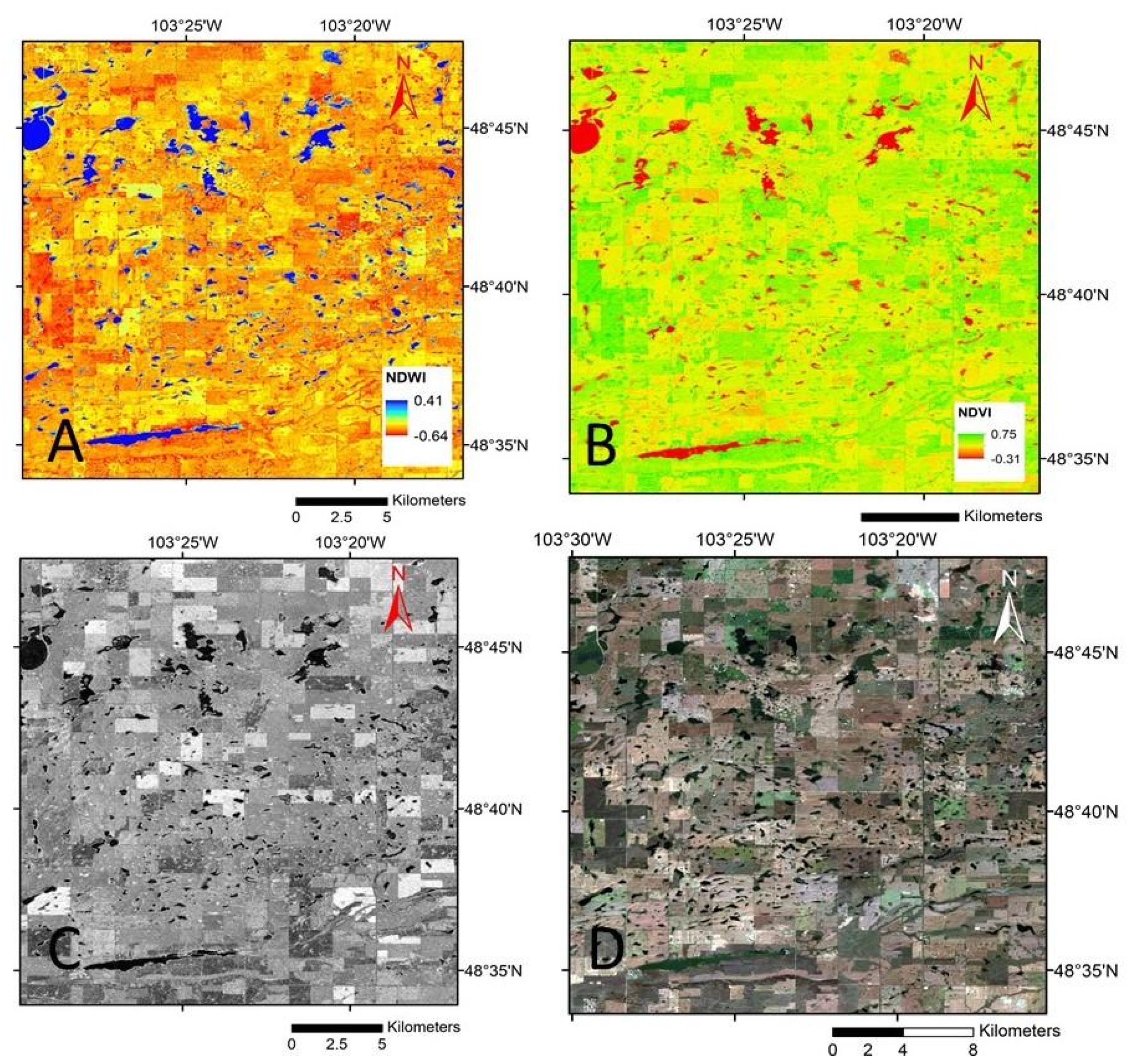
We used a total of 118 Sentinel-2 (S2) images with level 1C processing to surface reflectance as part of this study. S2 is a wide-swath multi-spectral earth observation mission with spatial resolution varying from 10 to 60 m. The multi-spectral data include 13 bands in the visible, near-infrared (NIR), and shortwave spectra, revisiting every 10 days under the same viewing angle. The level 1-C products within GEE are orthorectified and radiometrically corrected, providing top-of-atmosphere (TOA) reflectance values. We adopted an automatic cloud masking procedure using the QA60 band of the S2 1C product to mask the opaque and cirrus clouds. We also set the cloud coverage within S2 scenes to a maximum of 10 percent over the time of data acquisition. Due to frequent cloud coverage over the study area, we used a median of 5 months (May to October 2016) of the reflectance values. We used four bands of S2 (blue, green, red, and near-infrared) with a spatial resolution of 10 m to create the band compositions for supervised classifications using machine learning algorithms. We used median values of S2 temporal images to be used in the multisensory band composite. Additionally, we calculated the normalized difference vegetation index (NDVI) [33] and normalized difference water index (NDWI) [34] using the four bands of S2, and used them as predictors in the classification process (Figure 3). Figure 4 shows the variation of NDWI over two potholes in the study area, showing periods of inundation and drought. Typically, NDWI > 0.3 and <0.3 indicates the presence and absence of detectable surface water [35]
3.4. JRC Global Surface Water Products
This study focused on depressional wetlands that, by definition, are not permanent water, and often change inundation status quickly due to climate variability. We used the JRC product to differentiate wetlands from permanent water bodies across the entire study area. The Joint Research Centre’s Global Surface Water (JRC GSW) product contains the surface water’s spatial and temporal distribution at 30 m resolution. The product provides different characteristics of surface water, including occurrence, intensity, seasonality, recurrence, transitions, and maximum water extent [36]. The JRC GSW data were generated using more than 3 million scenes from various Landsat missions (Landsat 5, 7, and 8) between 1984 to 2019. The pixels were classified into water and non-water classes using an expert system. JRC GSW presents results each month for the entire period (1984–2019) for change detection. We defined permanent water bodies as those classified as water in >90% of the observations within the period (1984–2019), and filtered those pixels from the study. The permanent wet pixels were excluded from the final results to map the surface waters that only belong to wetlands.
4. Methods
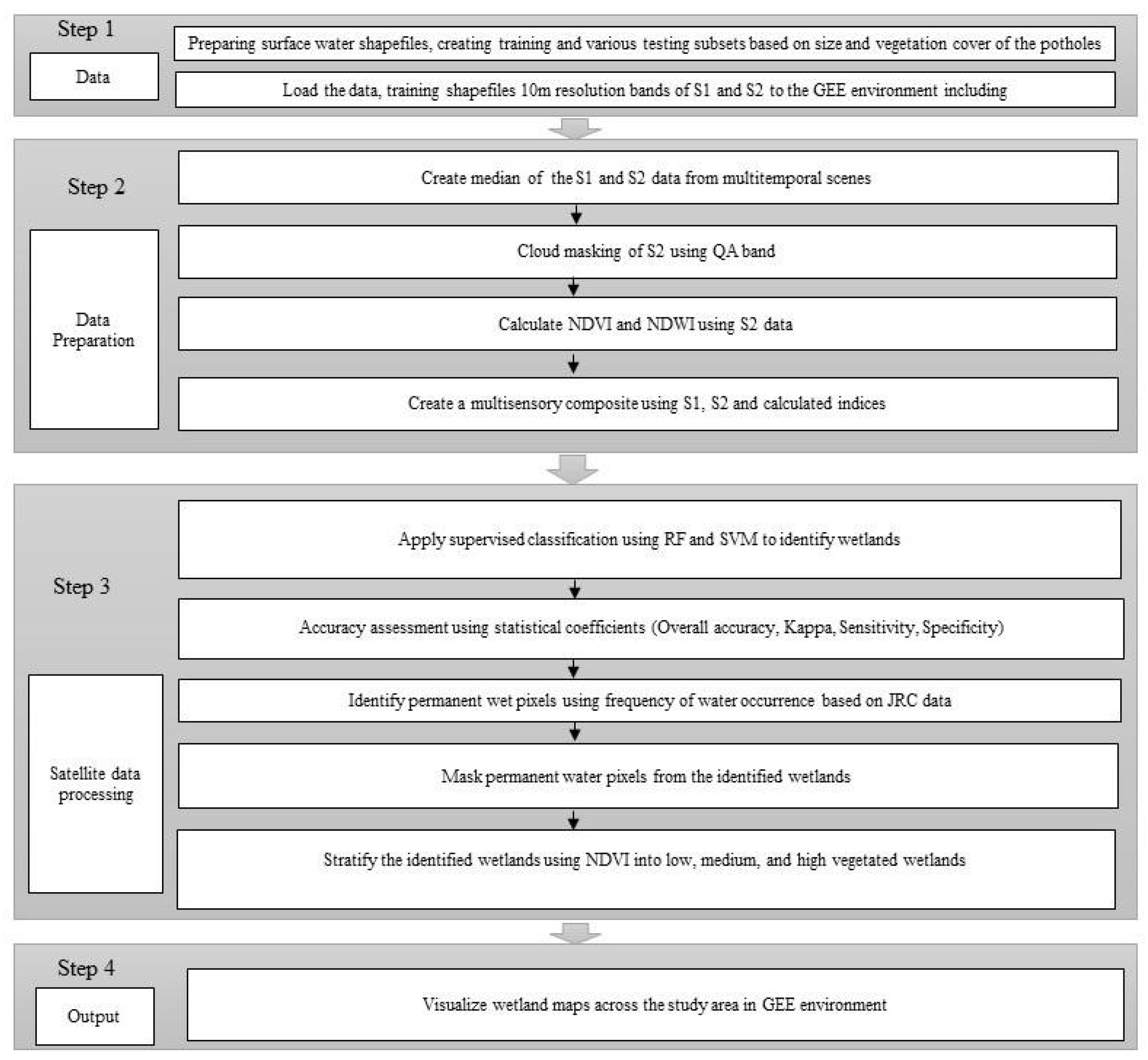
We developed an open-source process in GEE based on machine learning algorithms and multisensory remote sensing data for wetlands identification, as follows. First, a total of 895 ground truth points for 2016, including inundated wetlands and non-wetland classes, were randomly divided into two subsets of training (comprising 637 data points) and testing (comprising 258 data points). The training subset was used for training the machine learning algorithms, and the testing subset was withheld from the model, and used for the accuracy assessment. We created a multisensory band composite by integrating Sentinel-1 SAR data to selected Sentinel-2 high-resolution bands (Figure 3; Table 1). We used this Sentinel-1 and Sentinel-2 composite as predictors in the classification. We evaluated two machine learning algorithms, random forest (RF) and support vector machine (SVM), to establish a relationship between the multisensory composite bands as predictors and the training ground truth data. The optimum model (the model with the highest accuracy for classifying testing data) was used to classify the multisensory composite into two classes of wetlands and non-wetland pixels to identify wetlands in our study area. The generalizability of the optimum model was tested again using an additional 2231 ground truth points from a novel year, 2017.
Additionally, we tested the method by performing an accuracy assessment on small vegetated and small non-vegetated wetlands (see explanation below). Next, we excluded the permanent water bodies from the map using the JRC products as described above. Finally, we mapped the emergent vegetation within the identified wetlands using Sentinel-2-derived NDVI. We describe the details of the adopted methodology below. Figure 5 shows the workflow of the method.
4.1. Supervised Classification
Supervised machine learning algorithms establish relationships between input variables and target prediction [37,38,39]. We compared two popular machine learning algorithms, namely random forest (RF) and support vector machine (SVM), as supervised classifiers of surface water inundation, as predicted by the multisensory composite of Sentinel-1, Sentinel-2, NDVI, and NDWI (Table 1). These algorithms, which are available as functions within the GEE platform, were trained using the training subset, where the ground truth data served as a binary categorical response variable (0 = not an inundated wetland, 1 = inundated wetland). The trained algorithms were tested using the test subset, which was withheld from model fitting, and the model with the best performance was selected for the classification of the multisensory composite to identify the water bodies across the study area. The best performance was identified through accuracy assessment using statistical coefficients.
RF is an advanced version of a decision tree algorithm. Decision tree algorithms are robust predictive machine learning models that utilize a tree structure to establish relationships between inputs and outcomes. A tree structure mirrors how a tree starts at a wide trunk and splits into smaller branches as it is developed upward. Likewise, a decision tree learner uses a structure of branching decisions that lead examples into a final predicted class value. RF improves decision trees by combining bootstrap aggregation with random feature selection to add additional diversity to the model [40]. Further, though a decision tree is constructed on a whole dataset using all the features of interest, RF randomly selects observations and specific features to create multiple decision trees, and then averages the results to make predictions, which results in a more robust model [41]. The hyperparameters of the RF, including the number of trees, min leaf population, and bag fraction, were determined through a trial–error procedure in which we added the values gradually to obtain the least error values in the training data prediction outcome. The optimum hyperparameters of the RF model in this study are presented in Table 2.
The SVM classification tool uses machine learning theory to maximize predictive accuracy while automatically avoiding over-fitting the data [42]. SVM can be defined as systems that use the hypothesis space of linear functions in a high dimensional feature space, trained with a learning algorithm from the optimization theory [43]. SVM can be imagined as a surface that creates a boundary between plotted points in a multidimensional space representing their feature values. An SVM’s goal is to create a flat border, called a hyperplane, which divides the space to develop relatively homogeneous partitions on either side. We adjusted the hyperparameters needed for SVM through a trial–error procedure to identify the optimum structure of the SVM model (Table 2).
4.2. Identification of Wetland Surface Water
We used the 2017 testing data to estimate wetland surface water via the trained algorithm without refitting the model. As we mentioned before, the JRC product was used to exclude the permanent water pixels in order to identify surface water in wetlands across the test site. The remaining water pixels were stratified based on the presence of emergent vegetation, allowing us to determine the accuracy of detecting surface water in vegetated vs. non-vegetated wetlands, where vegetation status was inferred from NDVI values. The Jenks natural breaks optimization method was used to classify the wetlands into three low, medium, and high NDVI clusters (Table 3). The Jenks method is a data clustering technique designed to determine the best combination of values into different classes. This is performed by attempting to minimize the variance within classes, and maximize the variance between classes. NDVI values below zero typically represent open water [44], and increase with increasing vegetation cover until they saturate for high vegetation closed canopies [45].
4.3. Accuracy Assessment
The SVM and RF algorithms used to classify the multisensor composite were evaluated by constructing a confusion matrix for each model. The accuracy assessment was performed on the test subset in which the predictions and the ground truth data were compared using statistical coefficients (Equations (1–4)). Accuracy assessment was also carried out for the next year (2017) to evaluate the generalizability of the optimum model. The ground truth points for the year 2017 were only used for testing the model. Additionally, we performed separate accuracy assessments for small vegetated and small non-vegetated wetlands. To assess the accuracy of the methodology on small and highly vegetated wetlands, we provided a test set of 679 random points from small wetlands in the study area, with an additional 763 points from non-wetland classes from the 2016 aerial survey inventory. These were novel points that were not used as part of model training. These points came from wetlands with areas that ranged between 10 to 850 m2, and the presence of emergent vegetation ranged from 40 to 100%. We used the same procedure for small (10 to 850 m2) non-vegetated wetlands by providing a test set of 1680 points (1311 wetland and 369 non-wetland classes).
In the equations above, indicates the total number of observations; denotes the number of accurately classified wetland and non-wetland pixels; , , , and refer to true positive, true negative, false positive, and false negative, respectively.
where po is the relative observed agreement, and pe is the hypothetical probability of chance agreement:
and
5. Results
The trained SVM and RF algorithms were used to classify multisensor composites for the years 2016 and 2017. The accuracy assessment showed SVM and RF models yielded favorable results across the testing data. However, the RF outperformed the SVM in both 2016 and 2017 testing data. Therefore, the RF model was selected as the optimum model for wetland inundation mapping. The overall testing data accuracy for the SVM and RF model for the year 2016 was 0.88 and 0.95 (Table 4), and for the year 2017 was 0.88 and 0.94, respectively (Table 5). A summary of accuracy assessment using overall accuracy, Kappa, Sensitivity, and specificity for the years 2016 and 2017 is shown in Table 4 and Table 5, respectively.
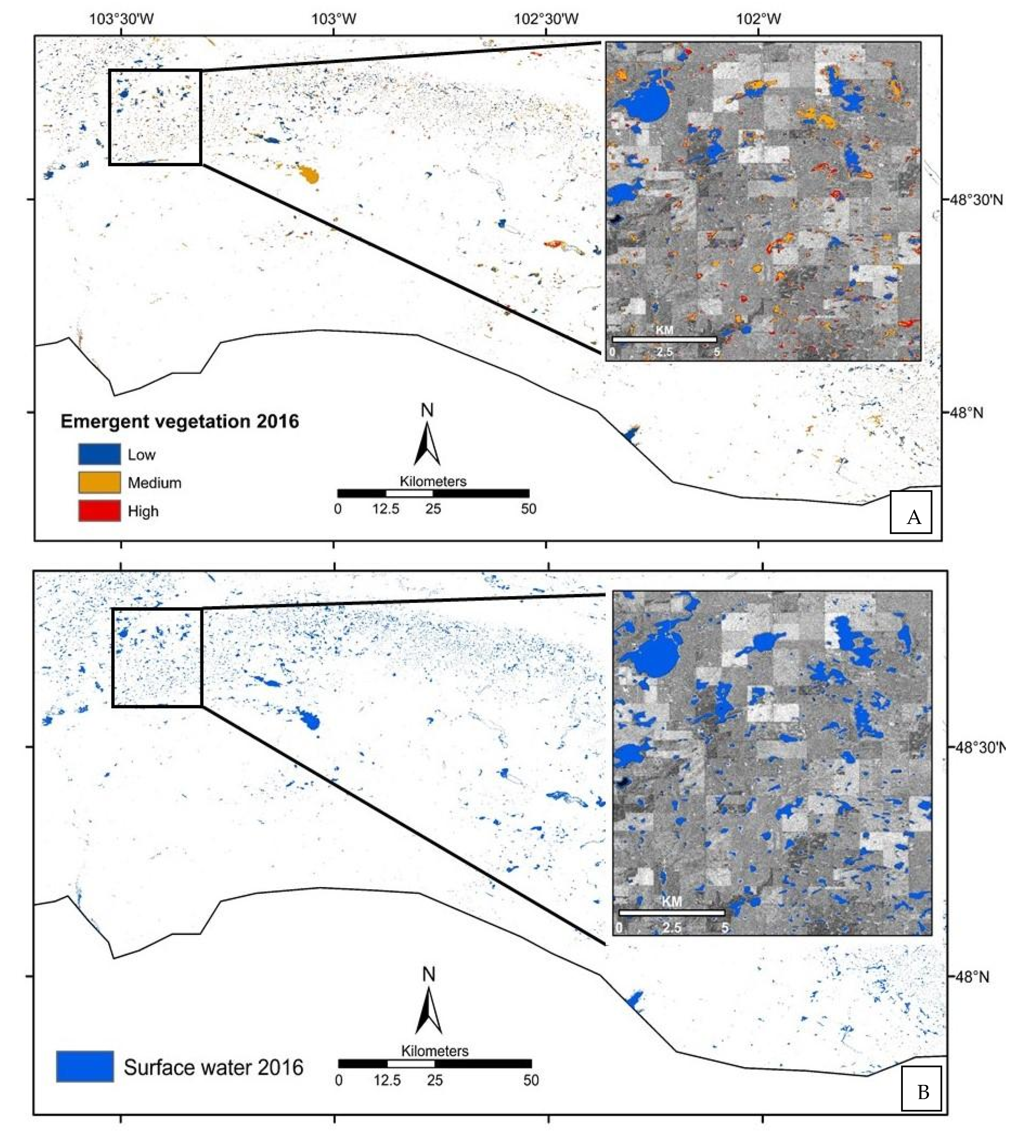
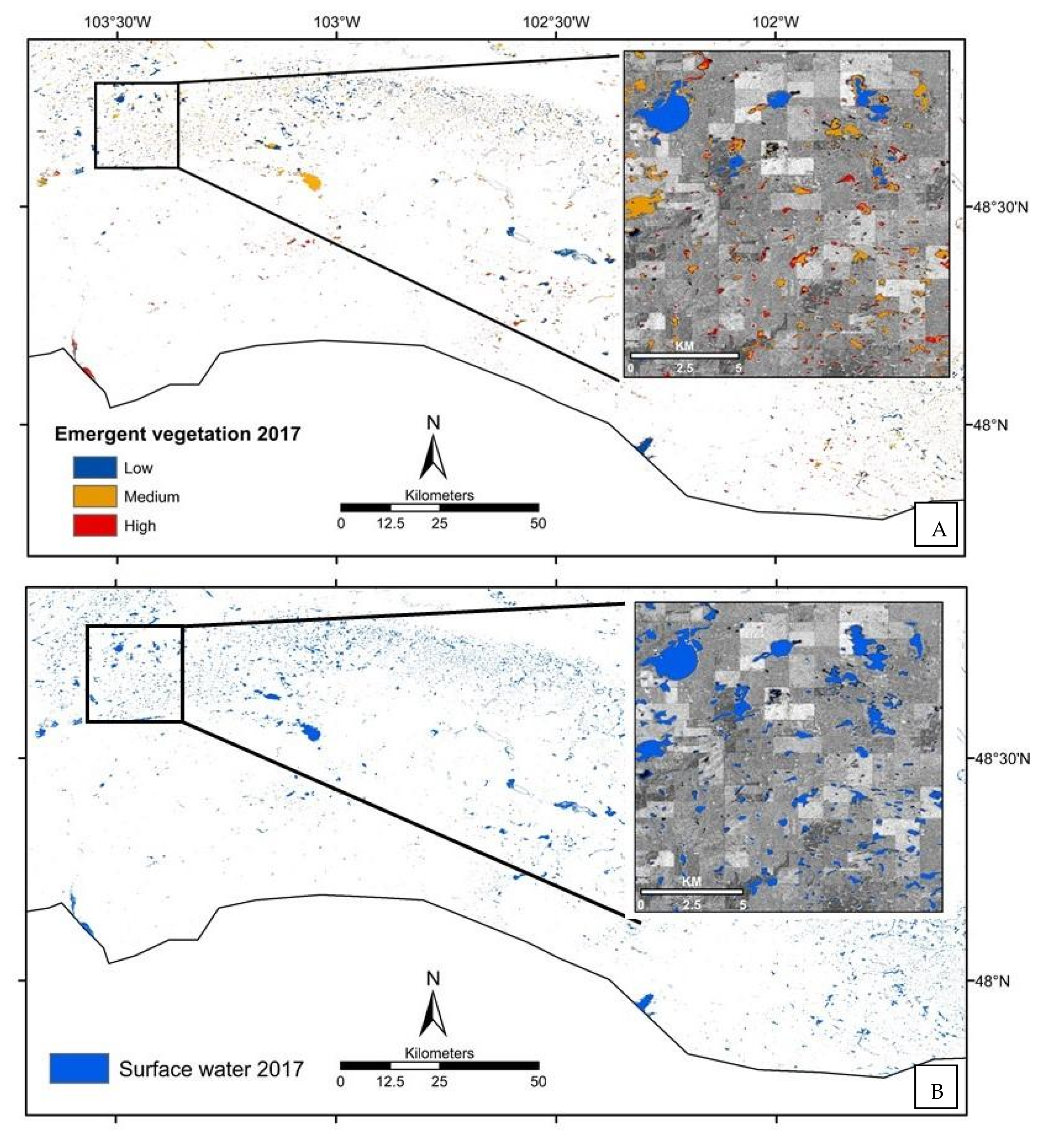
We mapped wetland surface water across the study area for the years 2016 and 2017. Figure 6 and Figure 7 show the identified wetlands across the study area for the years 2016 and 2017, respectively. The spatial resolution of the final maps is 10 m. The local wetland inundation in the study area can also be extracted based on the results. For example, a portion of the study area is magnified in Figure 8. A visual comparison between the aerial survey (ground truth data) and wetland surface water map (based on RF classifier) in Figure 9 shows that surface water in wetlands was mapped with acceptable accuracy (overall accuracy: 0.95; Kappa: 0.9). As we mentioned before, we also tested our algorithm in the identification of surface water in small vegetated and small non-vegetated wetlands. We compared the results with NDWI and Landsat-derived JRC surface water products (Table 6 and Table 7). The results showed higher accuracy in RF as the optimum model (overall accuracy 0.76) compared to JRC (overall accuracy 0.60) and NDWI (overall accuracy 0.62) in surface water detection in small and highly vegetated wetlands (Table 6). The RF (overall accuracy 0.81) also outperformed the NDWI (overall accuracy 0.44) and JRC (overall accuracy 0.41) in small non-vegetated wetlands (Table 7).
6. Discussion
This study developed an automated workflow within the GEE platform for mapping wetland surface water for 2016 and 2017 by applying the RF classifier to a combination of Sentinel-1, Sentinel-2 band data, and spectral reflectance indices derived from Sentinel-2. The results were evaluated using statistical coefficients and visual comparison with ground truth data, as well as results from Landsat-derived surface water products. The inundation of relatively large and deep water bodies can be identified in most existing remote sensing products. However, mapping wetland surface water in the PPR region is challenging due to two main reasons: (1) most PPR wetlands are very small and are highly sensitive to climate variability; and (2) the wetlands can be dry or wet, and they can contain different species of vegetation that can mask surface water. Therefore, these wetlands have complex spectral characteristics that complicate the detection of surface water extent from satellite sensors. Our approach also provides information regarding emergent vegetation within those wetlands. This is important because emergent vegetation provides shelter and food for aquatic vertebrates, such as waterfowl communities [46]. Our method can also detect water below those vegetation canopies; water that would otherwise be excluded from habitat maps. We also provide an open-science algorithm in GEE for repeating these estimates, which can form the basis of long-term wetland surface water monitoring in the PPR.
A typical approach for mapping wetlands uses passive remote sensing that relies on water’s optical properties, which differ from other land use types [47,48,49]. For instance, water quickly absorbs electromagnetic radiation, and more rapidly attenuates longer wavelengths than shorter ones [50,51,52]. However, the application of optical sensors in identifying PPR wetlands is limited, since both water depth and mixed pixels can change the water spectral signature [50,51,52]. Moreover, organic carbon compounds, water turbidity, chlorophyll content, and suspended materials can also add variation to water spectral properties. We addressed this issue by integrating the high-resolution bands of optical and radar sensors. Figure 9 shows a visual comparison of surface water derived from different remote sensing data. The figure shows that many small wetlands were not captured in the Landsat-derived surface water products, since the spatial resolution of Landsat products (30 m) is too coarse to capture those wetlands. This is typical of many surface water classifiers that are focused on deep open water, as they misclassify the highly variable spectral signatures of inundated wetlands [53]. Moreover, optical sensors struggled to capture wetlands covered by emergent vegetation. This study integrated Sentinel-1 SAR data into the high resolution (10 m) optical bands of Sentinel-2 to create a more robust classifier (Figure 9A). We also used a wider temporal window for the optical bands, which increased the number of observations over the study area. This allows our algorithm to minimize the effects of cloud covers, and identify the small wetlands by detecting frequently wet pixels. We performed an independent accuracy assessment on small and highly vegetated, and small non-vegetated wetlands. The results showed acceptable accuracy for both types of wetlands. We also compared the results with surface water maps derived from optical sensors (Table 6). Our algorithm performs better in identifying both large and small wetland water bodies than the Landsat-derived JRC and Sentinel-2-derived NDWI algorithms (Table 4, Table 5 and Table 6).
The wetland surface water was also evaluated in vegetated and non-vegetated wetlands. Visual observation shows that the small inundated wetlands contain more vegetation compared to larger and deeper water bodies. Comparing 2016 and 2017 wetland surface water maps reveals abrupt changes in emergent vegetation in small wetlands. These results agree with the findings of [54]. They reported that the small, ephemeral wetlands in the PPR experienced more vegetation change variability than larger, semi-permanent wetlands [54]. Large and deep water bodies can be easily detected by various remote sensing data. For example, [55] used Landsat time-series to create a global map of inland water dynamics. However, identifying small water bodies in the PPR is challenging due to the wetlands’ size and strong potential for dense vegetation cover. This is very important, as the majority of wetlands in the PPR are small. This causes the surface water in potholes to be highly dynamic. The total surface water area calculated from the JRC product and our classification method was 294 km2 and 376 km2, respectively. Algorithms that miss surface water in these small wetlands will be biased, and misrepresent the hydrologic variability on the landscape. For example, small wetlands provide more foraging habitats for organisms that rely on shallow water.
Cloud computing and the advent of multisensor remote sensing data in the GEE have several advantages for large-scale and time-series analysis, such as monitoring wetlands dynamics [56]. The use of the GEE cloud computing platform is more convenient than traditional methods, considering its processing speed and ease of use [57]. As more machine learning algorithms and remote sensing data become available within the GEE platform, we expect remote sensing data processing to be simplified even further. Additionally, and unlike most supercomputing centers, GEE is also designed to help researchers quickly disseminate their results to other researchers and interested parties. Once an algorithm has been developed on the GEE, users can generate systematic data products or deploy interactive applications aided by the GEE’s resources [25]. The fully automated workflow developed for this study allows us to refine the existing data and method, and rapidly apply it to a broad geographical scale to generate estimates in new years. One of the disadvantages of using the GEE cloud computing platform is that it limits the number of field samples and input features. This is especially challenging when the analysis is applied to a large domain, which may reduce the efficiency of the implemented method.
7. Conclusions
Wetland habitat characteristics, including wetland surface water area and vegetation presence, are essential for estimating waterfowl populations. The PPR contains millions of small wetlands providing abundant and critical habitats for waterfowl in North America. Mapping wetlands is needed to set conservation targets and develop management plans for waterfowl in the PPR. However, remote-sensing-based mapping of wetlands has previously been challenging. Many small wetlands in the region were missed by existing remote-sensing-derived surface water inventories due to limitations in the spatial resolution of remote sensing products. The trade-off between spectral and spatial resolution of remote sensing products necessitates the use of complementary data for wetland detection methods. Limiting the input parameters to the high-resolution bands of S2 helps detect smaller wetlands; however, it will ignore the spectral information of the other bands. Given its high resolution and ability to detect surface water, SAR can provide additional spectral information when combined with S2. The pre-processing of the original S1 and S2 images, and performing classification methods need massive computation. The GEE Cloud-based platform hosts many open access remote sensing images that provide remote analysis to apply machine learning algorithms for environmental monitoring. This study will share the resulting algorithm, which is tailored towards the needs of waterfowl conservation managers, with the management community, allowing its use for setting future conservation targets. These efforts will help conservation managers improve local estimates of pair abundance and waterfowl populations’ distribution patterns in the study area, and similar settings elsewhere.
Author Contributions
Conceptualization, H.S. and J.O.; Data curation, H.S. and K.M.K.; Formal analysis, H.S. and J.O.; Funding acquisition, J.O. and K.M.K.; Methodology, H.S. and J.O.; Software, H.S. and J.O.; Supervision, J.O.; Writing—original draft, H.S., J.O. and K.M.K.; Writing—review & editing, H.S., J.O. and K.M.K. All authors have read and agreed to the published version of the manuscript.
Funding
Ducks Unlimited, Inc and the United States Fish and Wildlife Service funded this project through the Prairie Pothole Joint Venture. The United States Fish and Wildlife Service Habitat and Population Evaluation Team provided ground truth data for surface water models.
Conflicts of Interest
The authors declare no conflict of interest.
References
- Gallant, A.L. The challenges of remote monitoring of wetlands. Remote Sens. 2015, 7, 10938–10950. [Google Scholar] [CrossRef] [Green Version]
- McLean, K.I.; Mushet, D.M.; Sweetman, J.N.; Anteau, M.J.; Wiltermuth, M.T. Invertebrate communities of Prairie-Pothole wetlands in the age of the aquatic Homogenocene. Hydrobiologia 2019, 20, 1–21. [Google Scholar] [CrossRef]
- Alonso, A.; Muñoz-Carpena, R.; Kaplan, D. Coupling high-resolution field monitoring and MODIS for reconstructing wetland historical hydroperiod at a high temporal frequency. Remote Sens. Environ. 2020, 247, 111807. [Google Scholar] [CrossRef]
- Jones, W.M.; Fraser, L.H.; Curtis, P.J. Plant community functional shifts in response to livestock grazing in intermountain depressional wetlands in British Columbia, Canada. Biol. Conserv. 2011, 144, 511–517. [Google Scholar] [CrossRef] [Green Version]
- Euliss, N.H.; LaBaugh, J.W.; Fredrickson, L.H.; Mushet, D.M.; Laubhan, M.K.; Swanson, G.A.; Nelson, R.D. The wetland continuum: A conceptual framework for interpreting biological studies. Wetlands 2004, 24, 448–458. [Google Scholar] [CrossRef]
- Leonard, P.B.; Baldwin, R.F.; Homyack, J.A.; Wigley, T.B. Remote detection of small wetlands in the Atlantic coastal plain of North America: Local relief models ground validation, and high-throughput computing. For. Ecol. Manag. 2012, 284, 107–115. [Google Scholar] [CrossRef]
- Batt, B.D.; Anderson, M.G.; Anderson, C.D.; Caswell, F.D. The use of prairie potholes by North American ducks. North. Prairie Wetl. 1989, 204, 227. [Google Scholar]
- Wu, Q.; Lane, C.R.; Li, X.; Zhao, K.; Zhou, Y.; Clinton, N.; DeVries, B.; Golden, H.E.; Lang, M.W. Integrating LiDAR data and multi-temporal aerial imagery to map wetland inundation dynamics using Google Earth Engine. Remote Sens. Environ. 2019, 228, 1–13. [Google Scholar] [CrossRef] [Green Version]
- Stewart, R.E.; Kantrud, H.A. Classification of Natural Ponds and Lakes in the Glaciated Prairie Region; US Bureau of Sport Fisheries and Wildlife: Fairfax County, VA, USA, 1971; Volume 92.
- Johnson, W.C.; Poiani, K.A. Climate change effects on prairie pothole wetlands: Findings from a twenty-five year numerical modeling project. Wetlands 2016, 36, 273–285. [Google Scholar] [CrossRef]
- Henry, B.L.; Wesner, J.S.; Kerby, J.L. Cross-ecosystem effects of agricultural tile drainage 2020, surface runoff, and selenium in the Prairie Pothole Region. Wetlands 2019, 40, 527–538. [Google Scholar] [CrossRef]
- Gleason, R.A.; Euliss, N.H., Jr. Sedimentation of prairie wetlands. Great Plains Res. 1998, 97–112. [Google Scholar]
- Leibowitz, S.G. Isolated wetlands and their functions: An ecological perspective. Wetlands 2003, 23, 517–531. [Google Scholar] [CrossRef]
- Euliss, N.H., Jr.; Gleason, R.A.; Olness, A.; McDougal, R.L.; Murkin, H.R.; Robarts, R.D.; Bourbonniere, R.A.; Warner, B.G. North American prairie wetlands are important nonforested land-based carbon storage sites. Sci. Total Environ. 2006, 361, 179–188. [Google Scholar] [CrossRef] [Green Version]
- Gholami, V.; Sahour, H.; Amri, M.A.H. Soil erosion modeling using erosion pins and artificial neural networks. Catena 2021, 196, 104902. [Google Scholar] [CrossRef]
- Guo, M.; Li, J.; Sheng, C.; Xu, J.; Wu, L. A review of wetland remote sensing. Sensors 2017, 17, 777. [Google Scholar] [CrossRef] [PubMed] [Green Version]
- Wright, C.; Gallant, A. Improved wetland remote sensing in Yellowstone National Park using classification trees to combine TM imagery and ancillary environmental data. Remote Sens. Environ. 2007, 107, 582–605. [Google Scholar] [CrossRef]
- Brooks, J.R.; Mushet, M.D.; Vanderhoof, M.K.; Leibowitz, S.G.; Christensen, J.R.; Neff, B.P.; Rosenberry, D.O.; Rugh, W.D.; Alexander, L.C. Estimating wetland connectivity to streams in the Prairie Pothole Region: An isotopic and remote sensing approach. Water Resour. Res. 2018, 54, 955–977. [Google Scholar] [CrossRef]
- Tulbure, M.G.; Broich, M. Spatiotemporal dynamic of surface water bodies using Landsat time-series data from 1999 to 2011. ISPRS J. Photogramm. Remote Sens. 2013, 79, 44–52. [Google Scholar] [CrossRef]
- Acharya, T.D.; Subedi, A.; Lee, D.H. Evaluation of water indices for surface water extraction in a Landsat 8 scene of Nepal. Sensors 2018, 18, 2580. [Google Scholar] [CrossRef] [Green Version]
- Huang, W.; DeVries, B.; Huang, C.; Lang, M.W.; Jones, J.W.; Creed, I.F.; Carroll, M.L. Automated extraction of surface water extent from Sentinel-1 data. Remote Sens. 2018, 10, 797. [Google Scholar] [CrossRef] [Green Version]
- Schlaffer, S.; Chini, M.; Pöppl, R.; Hostache, R.; Matgen, P. Monitoring of inundation dynamics in the North-American Prairie Pothole Region using Sentinel-1 time series. In Proceedings of the IGARSS 2018 IEEE International Geoscience and Remote Sensing Symposium, Valencia, Spain, 22–27 July 2018; pp. 6588–6591. [Google Scholar]
- Yan, J.; Ma, Y.; Wang, L.; Choo, K.K.R.; Jie, W. A cloud-based remote sensing data production system. Future Gener. Comput. Syst. 2018, 86, 1154–1166. [Google Scholar] [CrossRef] [Green Version]
- Fan, J.; Yan, J.; Ma, Y.; Wang, L. Big data integration in remote sensing across a distributed metadata-based spatial infrastructure. Remote Sens. 2018, 10, 7. [Google Scholar] [CrossRef] [Green Version]
- Gorelick, N.; Hancher, M.; Dixon, M.; Ilyushchenko, S.; Thau, D.; Moore, R. Google Earth Engine: Planetary-scale geospatial analysis for everyone. Remote Sens. Environ. 2017, 202, 18–27. [Google Scholar] [CrossRef]
- Kumar, L.; Mutanga, O. Google Earth Engine applications since inception: Usage trends, and potential. Remote Sens. 2018, 10, 1509. [Google Scholar] [CrossRef] [Green Version]
- Amarsaikhan, D.; Saandar, M.; Ganzorig, M.; Blotevogel, H.; Egshiglen, E.; Gantuyal, R.; Enkhjargal, D. Comparison of multisource image fusion methods and land cover classification. Int. J. Remote Sens. 2012, 33, 2532–2550. [Google Scholar] [CrossRef]
- Whyte, A.; Ferentinos, K.P.; Petropoulos, G.P. A new synergistic approach for monitoring wetlands using Sentinels-1 and 2 data with object-based machine learning algorithms. Environ. Model. Softw. 2018, 104, 40–54. [Google Scholar] [CrossRef] [Green Version]
- Roberts, D.; Mueller, N.; McIntyre, A. High-dimensional pixel composites from earth observation time series. IEEE Trans. Geosci. Remote Sens. 2017, 55, 6254–6264. [Google Scholar] [CrossRef]
- Cazals, C.; Rapinel, S.; Frison, P.L.; Bonis, A.; Mercier, G.; Mallet, C.; Corgne, S.; Rudant, J.P. Mapping and characterization of hydrological dynamics in a coastal marsh using high temporal resolution Sentinel-1A images. Remote Sens. 2016, 8, 570. [Google Scholar] [CrossRef] [Green Version]
- Brisco, B.; Short, N.; Sanden, J.V.D.; Landry, R.; Raymond, D. A semi-automated tool for surface water mapping with RADARSAT-1. Can. J. Remote Sens. 2009, 35, 336–344. [Google Scholar] [CrossRef]
- Lang, M.W.; Kasischke, E.S.; Prince, S.D.; Pittman, K.W. Assessment of C-band synthetic aperture radar data for mapping and monitoring Coastal Plain forested wetlands in the Mid-Atlantic Region USA. Remote Sens. Environ. 2008, 112, 4120–4130. [Google Scholar] [CrossRef]
- Pettorelli, N. The Normalized Difference Vegetation Index; Oxford University Press: Oxford, UK, 2013. [Google Scholar]
- Gao, B.C. NDWI—A normalized difference water index for remote sensing of vegetation liquid water from space. Remote Sens. Environ. 1996, 58, 257–266. [Google Scholar] [CrossRef]
- McFeeters, S.K. Using the normalized difference water index (NDWI) within a geographic information system to detect swimming pools for mosquito abatement: A practical approach. Remote Sens. 2013, 5, 3544–3561. [Google Scholar] [CrossRef] [Green Version]
- Pekel, J.F.; Cottam, A.; Gorelick, N.; Belward, A.S. High-resolution mapping of global surface water and its long-term changes. Nature 2016, 540, 418–422. [Google Scholar] [CrossRef]
- Gholami, V.; Khalili, A.; Sahour, H.; Khaleghi, M.R.; Tehrani, E.N. Assessment of environmental water requirement for rivers of the Miankaleh wetland drainage basin. Appl. Water Sci. 2020, 10, 1–14. [Google Scholar] [CrossRef]
- Sahour, H.; Gholami, V.; Vazifedan, M. A comparative analysis of statistical and machine learning techniques for mapping the spatial distribution of groundwater salinity in a coastal aquifer. J. Hydrol. 2020, 591, 125321. [Google Scholar] [CrossRef]
- Sahour, H.; Gholami, V.; Vazifedan, M.; Saeedi, S. Machine learning applications for water-induced soil erosion modeling and mapping. Soil Tillage Res. 2021, 211, 105032. [Google Scholar] [CrossRef]
- Breiman, L. Random Forests. Mach. Learn. 2001, 45, 5–32. [Google Scholar] [CrossRef] [Green Version]
- Sahour, H.; Gholami, V.; Torkaman, J.; Vazifedan, M.; Saeedi, S. Random forest and extreme gradient boosting algorithms for streamflow modeling using vessel features and tree-rings. Environ. Earth Sci. 2021, 80, 1–14. [Google Scholar] [CrossRef]
- Vapnik, V.N. An overview of statistical learning theory. IEEE Trans. Neural Netw. 1999, 10, 988–999. [Google Scholar] [CrossRef] [PubMed] [Green Version]
- Kanevski, M.; Pozdnoukhov, A.; Timonin, V. Machine Learning Algorithms for Geospatial Data. In Theory, Applications and Software; EPFL Press: Lausanne, Switzerland, 2009. [Google Scholar]
- Han, Q.; Niu, Z. Construction of the Long-Term Global Surface Water Extent Dataset Based on Water-NDVI Spatio-Temporal Parameter Set. Remote Sens. 2020, 12, 2675. [Google Scholar] [CrossRef]
- Petus, C.; Lewis, M.; White, D. Monitoring temporal dynamics of Great Artesian Basin wetland vegetation, Australia, using MODIS NDVI. Ecol. Indic. 2013, 34, 41–52. [Google Scholar] [CrossRef]
- Bradshaw, T.M.; Blake-Bradshaw, A.G.; Fournier, A.M.; Lancaster, J.D.; O’Connell, J.; Jacques, C.N.; Hagy, H.M. Marsh bird occupancy of wetlands managed for waterfowl in the Midwestern USA. PLoS ONE 2020, 15, e0228980. [Google Scholar] [CrossRef] [PubMed]
- Kayastha, N.; Thomas, V.; Galbraith, J.; Banskota, A. Monitoring wetland change using inter-annual landsat time-series data. Wetlands 2012, 32, 1149–1162. [Google Scholar] [CrossRef]
- Mao, D.; Wang, Z.; Du, B.; Li, L.; Tian, Y.; Jia, M.; Wang, Y. National wetland mapping in China: A new product resulting from object-based and hierarchical classification of Landsat 8 OLI images. ISPRS J. Photogramm. Remote Sens. 2020, 164, 11–25. [Google Scholar] [CrossRef]
- Wang, X.; Xiao, X.; Zou, Z.; Hou, L.; Qin, Y.; Dong, J.; Doughty, R.B.; Chen, B.; Zhang, X.; Chen, Y.; et al. Mapping coastal wetlands of China using time series Landsat images in 2018 and Google Earth Engine. ISPRS J. Photogramm. Remote Sens. 2020, 163, 312–326. [Google Scholar] [CrossRef] [PubMed]
- Cho, H.J.; Kirui, P.; Natarajan, H. Test of multi-spectral vegetation index for floating and canopy-forming submerged vegetation. Int. J. Environ. Res. Public Health 2008, 5, 477–483. [Google Scholar] [CrossRef] [PubMed] [Green Version]
- Ji, L.; Zhang, L.; Wylie, B. Analysis of dynamic thresholds for the normalized difference water index. Photogramm. Eng. Remote Sens. 2009, 75, 1307–1317. [Google Scholar] [CrossRef]
- O’Connell, J.L.; Mishra, D.R.; Cotten, D.L.; Wang, L.; Alber, M. The Tidal Marsh Inundation Index (TMII): An inundation filter to flag flooded pixels and improve MODIS tidal marsh vegetation time-series analysis. Remote Sens. Environ. 2017, 201, 34–46. [Google Scholar] [CrossRef]
- Jones, J.W. Efficient wetland surface water detection and monitoring via landsat: Comparison with in situ data from the everglades depth estimation network. Remote Sens. 2015, 7, 12503–12538. [Google Scholar] [CrossRef] [Green Version]
- Aronson, M.F.; Galatowitsch, S. Long-term vegetation development of restored prairie pothole wetlands. Wetlands 2008, 28, 883–895. [Google Scholar] [CrossRef]
- Pickens, A.H.; Hansen, M.C.; Hancher, M.; Stehman, S.V.; Tyukavina, A.; Potapov, P.; Marroquin, B.; Sherani, Z. Mapping and sampling to characterize global inland water dynamics from 1999 to 2018 with full Landsat time-series. Remote Sens. Environ. 2020, 243, 111792. [Google Scholar] [CrossRef]
- Amani, M.; Mahdavi, S.; Afshar, M.; Brisco, B.; Huang, W.; Mohammad Javad Mirzadeh, S.; Hopkinson, C. Canadian wetland inventory using Google Earth Engine: The first map and preliminary results. Remote Sens. 2019, 11, 842. [Google Scholar] [CrossRef] [Green Version]
- Huang, H.; Chen, Y.; Clinton, N.; Wang, J.; Wang, X.; Liu, C.; Zhu, Z. Mapping major land cover dynamics in Beijing using all Landsat images in Google Earth Engine. Remote Sens. Environ. 2017, 202, 166–176. [Google Scholar] [CrossRef]
Figure 1.
The location of the Prairie Pothole Region (PPR) (A); the location of the study site in the US and the state of North Dakota (B); distribution of ground truth points in the study site (C).
Figure 1.
The location of the Prairie Pothole Region (PPR) (A); the location of the study site in the US and the state of North Dakota (B); distribution of ground truth points in the study site (C).

Figure 2.
Spectral reflectance during summer months from Sentinel-2 optical bands of large bodies of deep open water compared to inundated wetlands and other land cover types in a portion of the study area. Wetland water shows different spectral characteristics compared to deep open water, likely due to the presence of submerged and emergent vegetation. The error bar shows the standard deviation of spectral reflectance of pixels for each land cover type.

Figure 3.
Sentinel-2 derived NDWI (A); NDVI (B); Sentinel-1 VV (C); Sentinel-2 RGB (D).

Figure 4.
An RGB image of Sentinel-2 over a portion of the study area (A). NDWI time series in two small potholes in the study area (B), and showing significant temporal variations in surface water (C).
Figure 4.
An RGB image of Sentinel-2 over a portion of the study area (A). NDWI time series in two small potholes in the study area (B), and showing significant temporal variations in surface water (C).

Figure 5.
Flowchart showing the main steps that were used in this study for mapping wetlands surface water.
Figure 5.
Flowchart showing the main steps that were used in this study for mapping wetlands surface water.

Figure 6.
Spatial distribution in inundated wetlands (A), spatial distribution of surface water (B) in August 2016.
Figure 6.
Spatial distribution in inundated wetlands (A), spatial distribution of surface water (B) in August 2016.

Figure 7.
Spatial distribution of emergent vegetation in inundated wetlands (A), spatial distribution of surface water (B) in August 2017.
Figure 7.
Spatial distribution of emergent vegetation in inundated wetlands (A), spatial distribution of surface water (B) in August 2017.

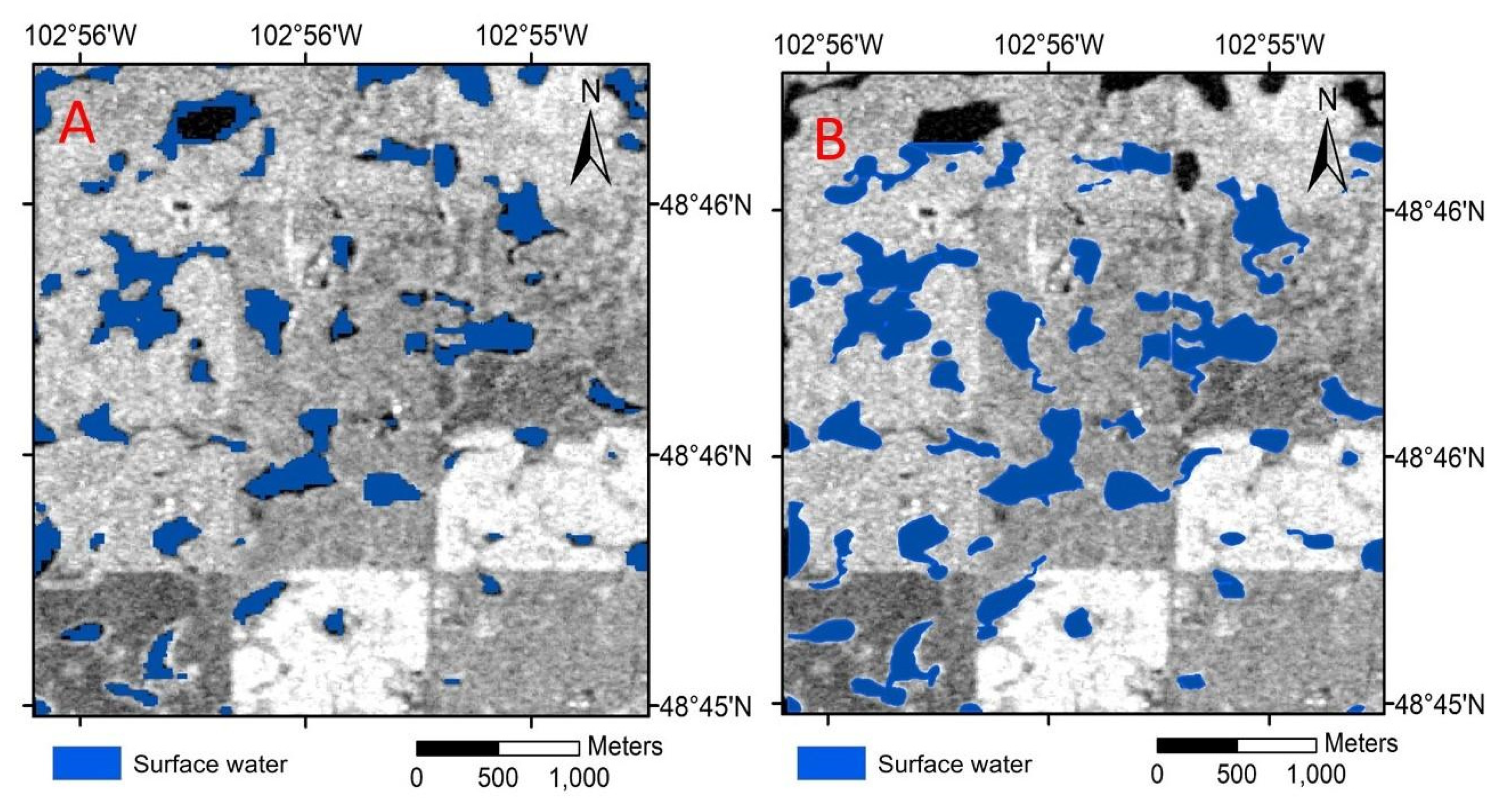
Figure 8.
Visual comparison of wetland inundation maps between predicted (A) and observed wetlands in aerial surveys (B) in a portion of the study area. The accuracy assessment for small vegetated wetlands and small non-vegetated wetlands are presented in Table 6 and Table 7, respectively.

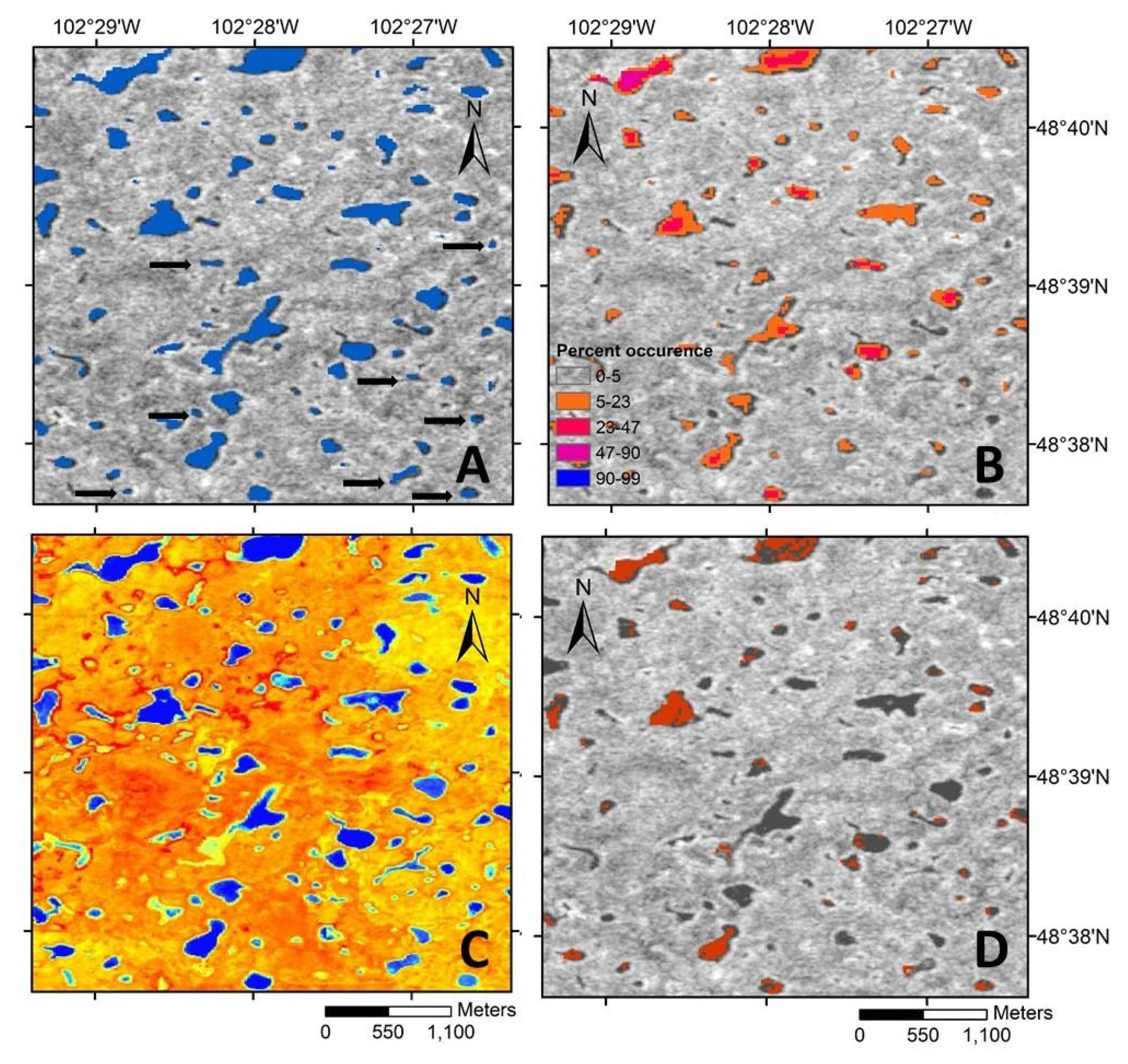
Figure 9.
The result of wetland inundation maps for the year 2017 was obtained from the multisensor composite classification using random forest. The image shows the identified wetland. The background image is Sentinel-1 VV. The black arrows show some examples of those small wetlands that were not detected in the JRC (A); frequency of surface water occurrence from the year 1984 to 2019 obtained from the Landsat-derived JRC products (B); surface water visualization using the Sentinel-2 derived NDWI (C); water extent for the year 2017 derived from the Landsat-derived JRC product (D).


Table 1.
Multisensor satellite data and spectral reflectance indices were used for supervised classification to identify the water bodies in the study area.
Table 1.
Multisensor satellite data and spectral reflectance indices were used for supervised classification to identify the water bodies in the study area.
| Data | Acquisition Date | Resolution (m) | Variable | Description |
|---|---|---|---|---|
| Sentinel-1 | July to September 2016 | 10 | VV | Backscattering coefficient for vertically polarized transmit and vertically polarized receive |
| Sentinel-1 | July to September 2016 | 10 | VH | Backscattering coefficient for vertically polarized transmit and horizontally polarized receive |
| Sentinel-2 | May to October 2016 | 10 | B2, B3, B4, B8 | Green, Blue, Red, Near-infrared |
| NDVI | May to October 2016 | 10 | (B8 − B4)/(B8 + B4) | Derived from Sentinel-2 bands |
| NDWI | May to October 2016 | 10 | (B3 − B8/(B3 + B8) | Derived from Sentinel-2 bands |
Table 2.
The optimum hyperparameters of the SVM and RF algorithms used for surface water classification.
Table 2.
The optimum hyperparameters of the SVM and RF algorithms used for surface water classification.
| SVM | RF | ||
|---|---|---|---|
| Parameter | Value | Parameter | Value |
| Kernel type | Radial basis function | Number of trees | 170 |
| Decision procedure | voting | Min Leaf Population | 1 |
| Hyper parameter gamma | 0.5 | Bag fraction | 0.5 |
| Cost C parameter | 10 | ||
Table 3.
NDVI cut-off values for classifying vegetation status in the identified wetlands.
| Class | NDVI Values | Cover Type |
|---|---|---|
| Low | −0.50 to 0.00 | Open water |
| Medium | 0.00 to 0.20 | Sparsely vegetated wetland |
| High | 0.20 to 0.77 | Densely vegetated wetland |
Table 4.
Accuracy assessment of supervised classification of wetland surface water (WSW) vs. other classes (OC) for the year 2016 on the test data subset that was withheld from model calibration.
Table 4.
Accuracy assessment of supervised classification of wetland surface water (WSW) vs. other classes (OC) for the year 2016 on the test data subset that was withheld from model calibration.
| Data | Overall Accuracy | Kappa | Sensitivity | Specificity | Correct WSW | Incorrect WSW | Correct OC | Incorrect OC |
|---|---|---|---|---|---|---|---|---|
| RF | 0.95 | 0.9 | 0.94 | 0.96 | 136 | 8 | 107 | 4 |
| SVM | 0.88 | 0.75 | 0.75 | 0.98 | 129 | 14 | 114 | 1 |
| JRC | 0.73 | 0.5 | 0.99 | 0.55 | 218 | 271 | 330 | 2 |
| NDWI | 0.68 | 0.38 | 0.67 | 0.48 | 287 | 89 | 184 | 305 |
Table 5.
Accuracy assessment of supervised classification of wetland surface water (WSW) vs. other classes (OC) for 2017 on the test data subset that was withheld from model calibration.
Table 5.
Accuracy assessment of supervised classification of wetland surface water (WSW) vs. other classes (OC) for 2017 on the test data subset that was withheld from model calibration.
| Data | Overall Accuracy | Kappa | Sensitivity | Specificity | Correct WSW | Incorrect WSW | Correct OC | Incorrect OC |
|---|---|---|---|---|---|---|---|---|
| RF | 0.94 | 0.87 | 0.9 | 0.99 | 757 | 250 | 1206 | 18 |
| SVM | 0.88 | 0.76 | 0.76 | 0.98 | 771 | 236 | 1205 | 19 |
| NDWI | 0.7 | 0.36 | 0.72 | 0.86 | 584 | 423 | 1131 | 93 |
| JRC | 0.72 | 0.41 | 0.99 | 0.75 | 612 | 395 | 1178 | 2 |
Table 6.
Accuracy assessment for detection of wetland surface water (WSW) vs. other classes (OC) in wetlands that are both small (<850 m2) and highly vegetated wetlands (vegetation > 40%) from the year 2016 on the test data subset that was withheld from model calibration.
Table 6.
Accuracy assessment for detection of wetland surface water (WSW) vs. other classes (OC) in wetlands that are both small (<850 m2) and highly vegetated wetlands (vegetation > 40%) from the year 2016 on the test data subset that was withheld from model calibration.
| Data | Overall Accuracy | Kappa | Sensitivity | Specificity | Correct WSW | Incorrect WSW | Correct OC | Incorrect OC |
|---|---|---|---|---|---|---|---|---|
| RF | 0.76 | 0.51 | 0.97 | 0.69 | 342 | 334 | 753 | 10 |
| SVM | 0.73 | 0.44 | 0.84 | 0.68 | 324 | 352 | 694 | 69 |
| NDWI | 0.62 | 0.19 | 0.94 | 0.58 | 131 | 545 | 755 | 8 |
| JRC | 0.6 | 0.15 | 1 | 0.57 | 99 | 577 | 763 | 0 |
Table 7.
Accuracy assessment for detection of wetland surface water (WSW) vs. other classes in small (<850 m2) and non-vegetated (vegetation < 40%) wetlands for 2016.
Table 7.
Accuracy assessment for detection of wetland surface water (WSW) vs. other classes in small (<850 m2) and non-vegetated (vegetation < 40%) wetlands for 2016.
| Data | Overall Accuracy | Kappa | Sensitivity | Specificity | Correct WSW | Incorrect WSW | Correct OC | Incorrect OC |
|---|---|---|---|---|---|---|---|---|
| RF | 0.81 | 0.57 | 0.98 | 0.55 | 1027 | 287 | 344 | 25 |
| SVM | 0.72 | 0.41 | 0.97 | 0.43 | 858 | 456 | 346 | 23 |
| NDWI | 0.44 | 0.14 | 0.99 | 0.28 | 379 | 941 | 365 | 4 |
| JRC | 0.41 | 0.13 | 1 | 0.27 | 324 | 987 | 368 | 1 |
Publisher’s Note: MDPI stays neutral with regard to jurisdictional claims in published maps and institutional affiliations. |
© 2021 by the authors. Licensee MDPI, Basel, Switzerland. This article is an open access article distributed under the terms and conditions of the Creative Commons Attribution (CC BY) license (https://creativecommons.org/licenses/by/4.0/).
Share and Cite
MDPI and ACS Style
Sahour, H.; Kemink, K.M.; O’Connell, J. Integrating SAR and Optical Remote Sensing for Conservation-Targeted Wetlands Mapping. Remote Sens. 2022, 14, 159. https://doi.org/10.3390/rs14010159
AMA Style
Sahour H, Kemink KM, O’Connell J. Integrating SAR and Optical Remote Sensing for Conservation-Targeted Wetlands Mapping. Remote Sensing. 2022; 14(1):159. https://doi.org/10.3390/rs14010159
Chicago/Turabian StyleSahour, Hossein, Kaylan M. Kemink, and Jessica O’Connell. 2022. "Integrating SAR and Optical Remote Sensing for Conservation-Targeted Wetlands Mapping" Remote Sensing 14, no. 1: 159. https://doi.org/10.3390/rs14010159
Note that from the first issue of 2016, this journal uses article numbers instead of page numbers. See further details here.