Hyperspectral Remote Sensing Detection of Marine Oil Spills Using an Adaptive Long-Term Moment Estimation Optimizer

Abstract

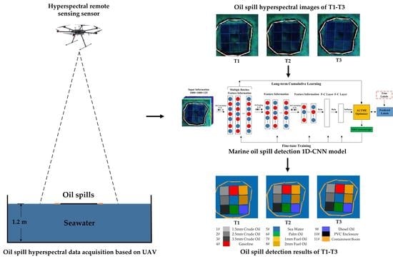
Marine oil spills can damage marine ecosystems, economic development, and human health. It is important to accurately identify the type of oil spills and detect the thickness of oil films on the sea surface to obtain the amount of oil spill for on-site emergency responses and scientific decision-making. Optical remote sensing is an important method for marine oil-spill detection and identification. In this study, hyperspectral images of five types of oil spills were obtained using unmanned aerial vehicles (UAV). To address the poor spectral separability between different types of light oils and weak spectral differences in heavy oils with different thicknesses, we propose the adaptive long-term moment estimation (ALTME) optimizer, which cumulatively learns the spectral characteristics and then builds a marine oil-spill detection model based on a one-dimensional convolutional neural network. The results of the detection experiment show that the ALTME optimizer can store in memory multiple batches of long-term oil-spill spectral information, accurately identify the type of oil spills, and detect different thicknesses of oil films. The overall detection accuracy is larger than 98.09%, and the Kappa coefficient is larger than 0.970. The F₁-score for the recognition of light-oil types is larger than 0.971, and the F₁-score for detecting films of heavy oils with different film thicknesses is larger than 0.980. The proposed optimizer also performs well on a public hyperspectral dataset. We further carried out a feasibility study on oil-spill detection using UAV thermal infrared remote sensing technology, and the results show its potential for oil-spill detection in strong sunlight.

1. Introduction

With the rapid development of the global marine transportation and offshore oil extraction industries, marine oil spills frequently occur, which seriously affects the sustainable development of the marine ecological environment and resources. The accurate identification and analysis of the type of marine oil spills are helpful for determining the responsibility for accidents and are extremely important for on-site emergency responses and the rapid and effective treatment of sea surface pollution. Obtaining an accurate value for the oil film thickness and then estimating the amount of oil spill is an important basis for accountability in pollution compensation, which plays an important role in scientific decision-making and determining the severity of the oil-spill accident [1,2]. Oil-spill type identification and oil-film thickness detection via remote sensing are popular topics at the frontier of current research on oil-spill optical remote sensing, which remains susceptible to cloud and fog conditions [3,4,5,6]. Unmanned aerial vehicle (UAV) optical remote sensing technology has been used for the disposal of oil-spill accidents in recent years because it can quickly and effectively acquire remote sensing data of marine oil spills [7,8].

Lammoglia used laboratory measurements to obtain the spectral data of different oil types, developed a series of feature extraction and identification methods for different oil types based on principal component analysis, and established an oil type spectral library. Experiments have shown that the spectral absorption characteristics of crude and fuel oils are obvious, but the effective identification of different types of light oils has not yet been achieved [9,10,11]. The current standard for crude oil film thickness evaluation is the Bonn protocol, which is recognized by the International Maritime Organization. The main problem with the protocol is that the oil film identification is strongly affected by subjective and environmental factors, and it is impossible to distinguish between thick oil films larger than 100 µm [12,13]. Lu’s experimental results show that within a certain range, the absolute thickness of the oil film has a positive linear relationship with the level of brightness temperature, but the upper limit of this detection method is 400 µm [14]. Lu further measured oil emulsion spectra in a laboratory environment to obtain non-imaging ASD hyperspectral data of crude oil emulsions that can fully represent the backscattering characteristics as well as C-H and O-H absorption characteristics [15]. A hyperspectral remote sensing identification method of oil emulsion based on a decision tree was proposed, and good experimental results were obtained [16].

An oil spill is a weak target in optical remote sensing research, and it is difficult to distinguish the spectral curves of different types of light oils. Traditional remote sensing modeling methods based on characteristic bands have made positive progress with heavy oils, but the research on identifying light oil types has been mostly carried out in a laboratory environment, and the performance of the proposed methods is not ideal [17,18,19,20,21,22,23]. In addition, the oil film of heavy oil has a strong absorption effect on sunlight, so the remote sensing reflectance is lower than light oils, and the spectral separability of oil films with different thicknesses is poor. Therefore, it is difficult to detect the thickness of thick oil film based on optical remote sensing. At present, the research in oil film thickness is mostly based on the inversion of thin or relative thickness based on traditional remote sensing modeling methods, and the research on the detection of the absolute thickness of thick oil film has not been adequately investigated [24,25,26,27].

Hyperspectral remote sensing has the characteristics of high spectral resolution and a wide spectral response range. In contrast to traditional multi-spectral remote sensing technology, it can obtain rich oil-spill spectral characteristic information [28,29,30]. Moreover, deep learning has developed rapidly in recent years because of its powerful ability to extract features from high-dimensional data [31,32,33,34,35,36,37]. Deep networks and multi-level features fusion method for deep learning have been applied to hyperspectral image classification, and research progress has been made [38,39,40]. In this paper, the combination of hyperspectral remote sensing technology and deep learning is conducive to extracting the spectral characteristic information and then accurately identifying the type of oil spills and detecting thick oil films with different thicknesses.

At present, marine oil-spill detection based on remote sensing mostly lacks on-site measured data to carry out accurate accuracy verification of detection methods [41,42]. In this study, an outdoor experimental setup was built to simulate a real marine oil-spill environment. By adding experimental oil qualitatively and quantitatively to the experimental scene, the accuracy of the detection results of the oil spill experiment will be evaluated. Compared to non-imaging oil spill hyperspectral studies, we collected airborne hyperspectral remote sensing images of five types of oil spills (crude oil, fuel oil, gasoline, diesel, and palm oil), crude oil, and fuel oil with different thicknesses at three different times.

The traditional adaptive moment estimation (Adam) optimizer, which is widely used in various deep learning tasks, uses the mechanism of an exponential moving average to update the second momentum term and then update the model weight. When applied to the hyperspectral oil-spill images in this experiment, the oil-spill spectral characteristic information would be lost, which would affect the oil-spill detection performance [43,44,45]. We combine UAV hyperspectral remote sensing technology with deep learning and propose an adaptive long-term moment estimation (ALTME) optimizer which can meet the characteristics of hyperspectral imagery and adapt to different phases of oil-spill scenes. To realize the cumulative learning function of the optimizer for multi-batch and long-term historical spectral characteristic information, we integrate the proposed optimizer with a one-dimensional convolutional neural network (1D-CNN); we consequently extracted the oil-spill spectral characteristic information obtained by the hyperspectral remote sensing data using 1D convolution. The aim of the marine oil-spill 1D-CNN detection model is to improve the detection performance of oil-spill types and thick oil films, and it is expected to be applied in future research on the detection of marine oil spills.

2. Data and Method

2.1. Data

The experiment lasted for four days, from 19 to 22 September 2020. We conducted the experiment in the large-scale land-based experimental pool of Qingdao Scientific Research Base, China, which is 50 m long, 40 m wide, and 2 m deep. There is no shade during the day, and the lighting conditions are good. About 20 m to the west of the pool is the Yellow Sea shore, which facilitates the extraction of seawater required for the experiment. An aerial photograph of the experimental land-based pool is shown in Figure 1.

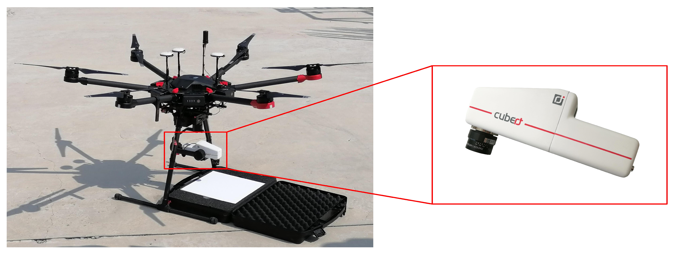
In this experiment, a Cubert-S185 hyperspectral sensor (Cubert, Berlin, Germany) was used to obtain the hyperspectral images of the oil spills on the sea surface. The radiometric calibration plate is AZ-WS20, and its manufacturer is Sphereoptics from the Washington, DC, USA. DJI-M600PRO UAV is equipped with an A3Pro flight control system and Zenmuse gimbal, which has good stability and balance ability. The sensor was installed on a DJI-M600PRO UAV, as shown in Figure 2.

The Cubert-S185 hyperspectral sensor uses a frame imaging mode; it has a spectral range of 450–950 nm, a spectral resolution of 4 nm, and 125 bands. The specifications of the Cubert-S185 sensor and M600PRO UAV are listed in

Table 1. Specifications of Cubert-S185 Hyperspectral Sensor and DJI-M600PRO UAV.

Parameter		Index
Cubert-S185	Spectral range (nm)	450~950
	Spectral resolution (nm)	4
	Number of bands	125
	IFOV (°)	23
	Imaging method	Frame imaging
	Imaging size (pixel)	1000 × 1000
M600PRO	Maximum load (kg)	6
	Flight duration (min)	16
	Maximum wind resistance level (m/s)	8
	Maximum ascent/descend speed (m/s)	5/3
	Maximum flight altitude (m)	4500
	Maximum horizontal speed (km/h)	65

. In addition, using the 12 megapixels CMOS optical imaging system carried by DJI-Mavic2 UAV, we collected high-resolution optical images of the oil spills to assist the ground-truth labeling of the hyperspectral images so as to carry out accuracy verification of the detection model proposed in this paper.

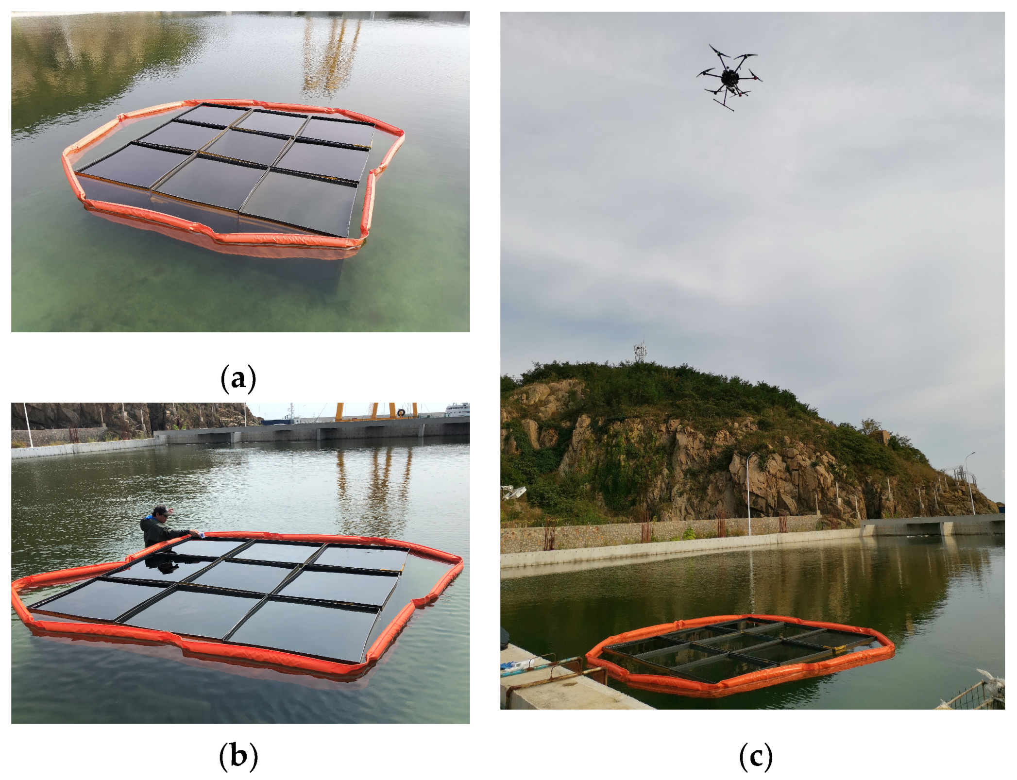
While ensuring the safety of the experiment, our aim was to simulate a real marine oil-spill accident scene as closely as possible. Because the experiment involves the identification of oil-spill types and the detection of oil films with different thicknesses, to carry out qualitative remote sensing analysis more ideally, we built an experimental enclosure using a PVC (Polyvinyl Chloride) board. The PVC enclosure was sealed and reinforced with high-strength glass glue and hinges to prevent the oil films from spreading irregularly on the water surface, and an image of its construction is shown in Figure 3. The experimental enclosure has a height of 1.2 m and consists of nine small enclosures. The size of each small enclosure was 1 × 1 m, which we labeled as groups 1–9 in turn. Because the experimental site is close to the Yellow Sea and Laoshan Bathing Beach, to reduce the risk of oil spills, we set up an oil containment boom around the experimental device to prevent oil films leakage, as shown in Figure 4.

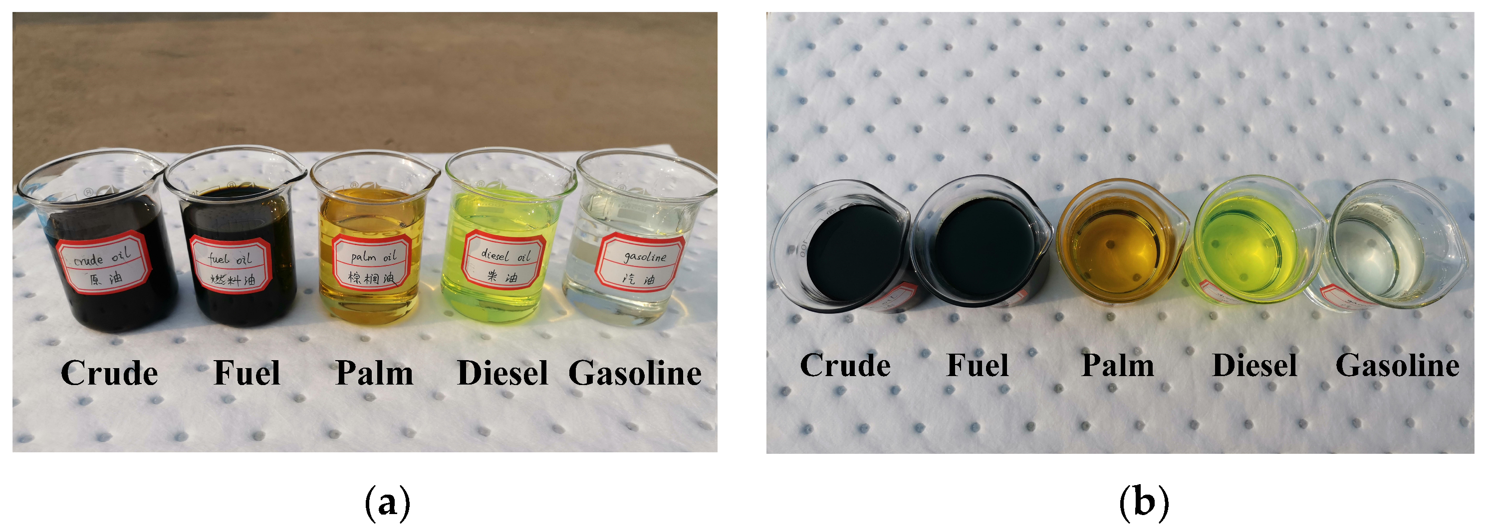
The oils used in this experiment are shown in Figure 5. From left to right are crude oil from the Dongying Shengli Oilfield, fuel oil, edible palm oil, diesel (#0), and gasoline (#95). The heavy-oil experimental groups included crude oil and fuel oil, and the light-oil experimental groups included palm oil, diesel, and gasoline.

The Bonn protocol distinguishes in detail the thin oil films of crude oils smaller than 0.1 mm (the protocol has seven levels), whereas the distinction for black oil slicks of 0.5–4 mm is rough (only two levels are used). Our aim was to investigate the hyperspectral remote sensing detection of thick heavy-oil films. Hence, we set the absolute thicknesses of the crude oil films in the experiment to be approximately 1.5 mm, 2.5 mm, and 3.5 mm, with thickness intervals of 1 mm. The absolute thickness of the fuel oil films was set to approximately 1 mm and 2 mm with a thickness interval of 1 mm. In this study, we regarded oil films with different thicknesses as different thickness grades to explore the capabilities of the airborne hyperspectral remote sensing technology to qualitatively detect thick heavy-oil films.

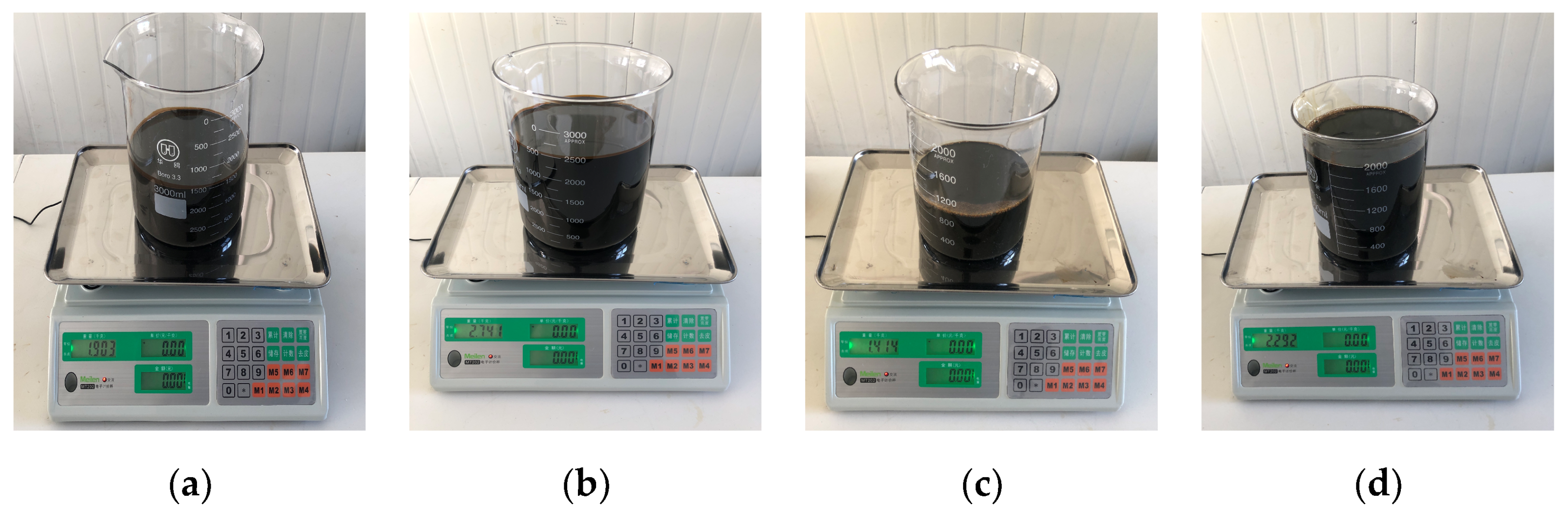
In this study, under the same experimental environment, the density of the crude and fuel oils was calculated to be 0.81 kg/L and 0.85 kg/L, respectively. A pallet balance (with an accuracy of 0.001 kg) was used to calculate the quality of the experimental oil by measuring the difference before and after it was poured into the experimental enclosure, and then the volume was obtained based on the density of the oil. The weighing process of crude oil and fuel oil is shown in Figure 6.

The size of each small enclosure (S_E) in the experiment is known to be 1 m². We used large-capacity beakers (2 L and 3 L) to control the volume of oil poured into the experimental enclosure. We then calculated the absolute thickness of the oil films of the heavy-oil experimental groups using

$$h_{\mathrm{Oil}}=\frac{M_1-M_2}{{\rho }_{\mathrm{Oil}}·S_{\mathrm{E}}}$$

(1)

where M₁ is the mass of the beaker before adding the experimental oil, M₂ is the mass of the beaker after adding the oil, ρ_Oil is the density of the oil, and h_Oil is the absolute thickness of the oil film.

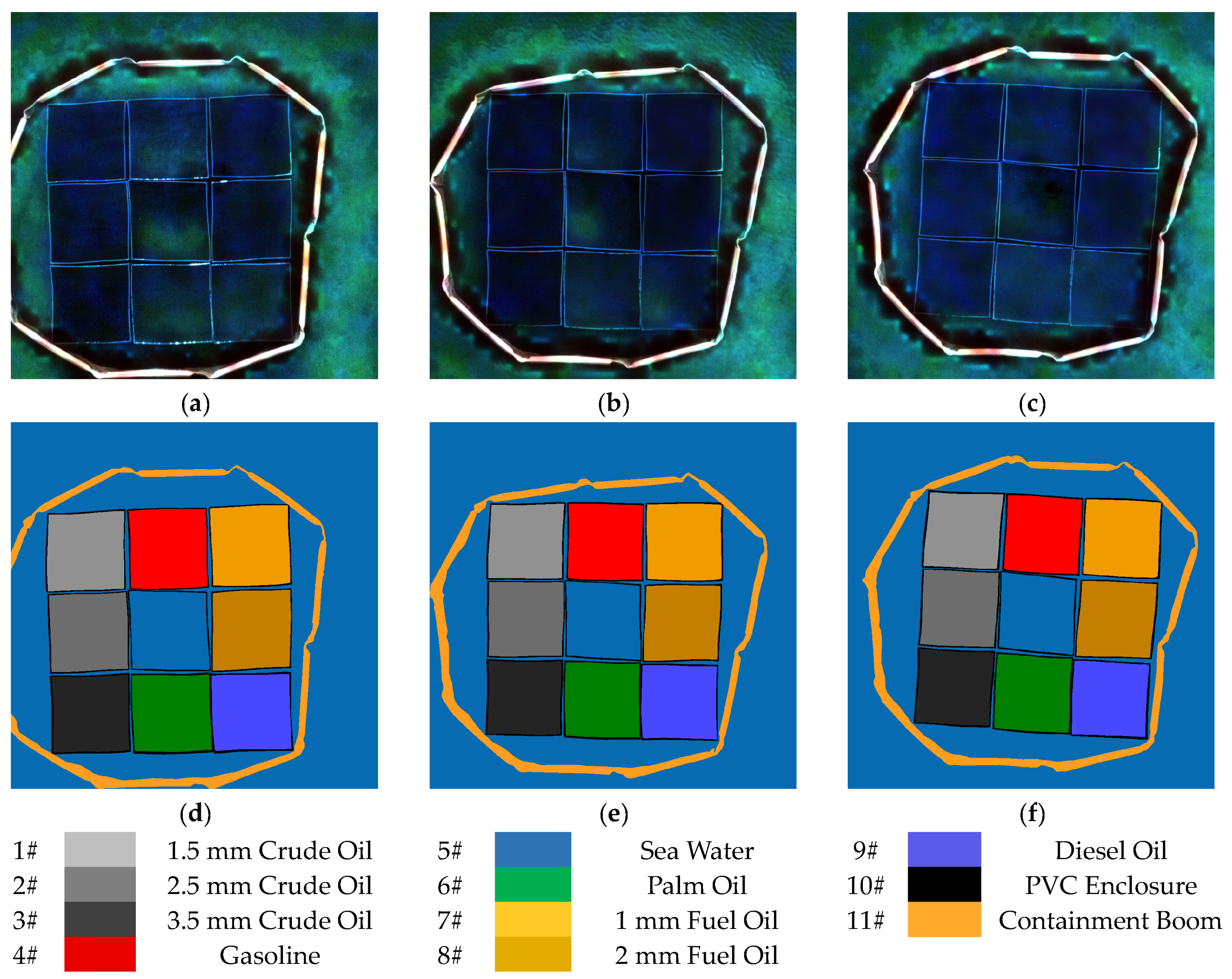
With the exception of group 5, which was seawater without any experimental oil, we poured crude oil into groups 1–3, #95 gasoline into group 4, palm oil into group 6, fuel oil into groups 7–8, and #0 diesel into group 9 in the experimental enclosure in sequence to obtain oil-spill observation scenes of the different types of light oils and heavy-oil films with different thicknesses. The measured data of the heavy-oil film experimental groups is given in

Table 2. Data of the heavy-oil film experiment groups.

Group	M1 (kg)	M2 (kg)	M (kg)	ρOil (kg/L)	V (L)	hOil (mm)
1#-1.5 mm Crude	1.90	0.66	1.24	0.81	1.53	1.53
2#-2.5 mm Crude	2.74	0.65	2.09	0.81	2.58	2.58
3#-3.5 mm Crude	4.10	1.21	2.89	0.81	3.57	3.57
7#-2 mm Fuel Oil	1.41	0.58	0.83	0.85	0.98	0.98
8#-3 mm Fuel Oil	2.30	0.58	1.72	0.85	2.06	2.06

.

After uniform diffusion of the oil films, using the calibrated Cubert-S185 hyperspectral sensor carried by the DJI-M600PRO UAV, we obtained hyperspectral images of the oil films in the enclosure at 11:30 h (T1), 14:00 h (T2), and 16:30 h (T3). In this experiment, we took the flying method of avoiding the sun glint to avoid the influence of the sun glint. The time intervals between T1, T2, and T3 are all 2.5 h, and the experimental process of data acquisition is shown in Figure 7.

Environmental data such as wind speed and temperature were obtained with a Kestrel-3500 meteorological instrument (

Table 3. Environmental data of the experiment.

Moment	Wind Speed (m/s)	Cross Wind (m/s)	Upwind (m/s)	Temp (°C)	Solar Elevation Angle (°)	Solar Azimuth Angle (°)	Weather
11:30	0.80	0.70	−0.30	26.80	53.82	12.77	Sunny
13:50	1.50	0.80	1.30	26.90	45.92	−41.59	Sunny
16:21	1.80	1.00	1.50	24.50	19.84	−74.89	Sunny

). During the UAV hyperspectral remote sensing data collection, the weather was clear, and there was no cloud or fog obstruction. From T1 to T3, the wind speed gradually increased, but the overall wind speed and wind speeds in all directions were below 2 m/s, which is classed as “light air” according to the Beaufort Scale, and the sea was relatively calm.

In this study, using Python and the Cubert-Touch platform, radiometric calibration, and remote sensing reflectance calculation were carried out on the hyperspectral images of the oil spills obtained by the airborne Cubert-S185 sensor. The calculation is as follows.

$$R_{\mathrm{rs}}=\frac{L_{\mathrm{w}}}{\mathsf{\pi }·L_{\mathrm{p}}}$$

(2)

Here, R_rs represents the oil spill’s remote sensing reflectance, L_w is the oil spill’s radiometric data obtained by the S185 hyperspectral sensor, L_p represents the radiometric data of the AZ-WS20 calibration plate.

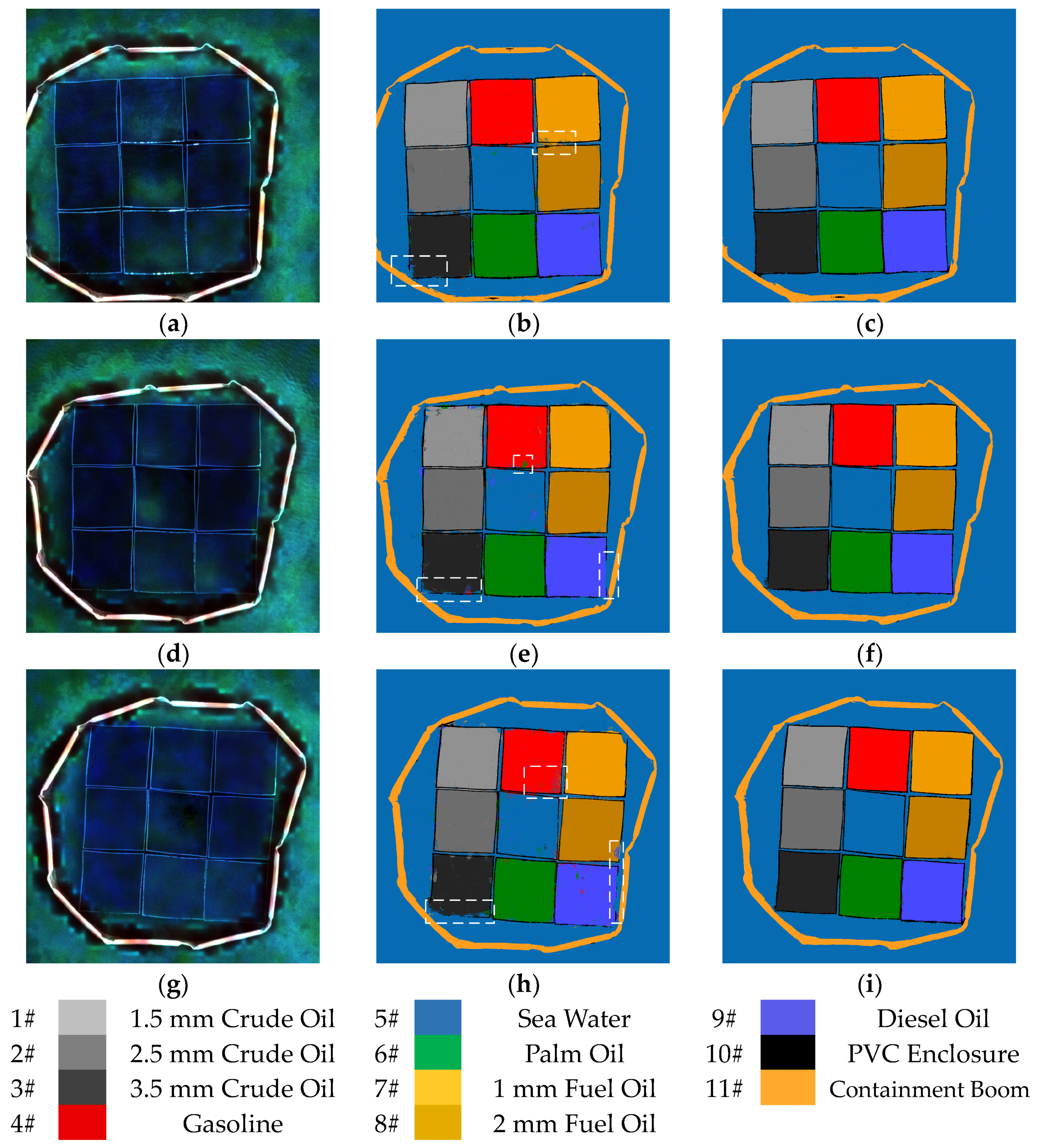
We used the 12-megapixel CMOS sensor mounted on the DJI-Mavic2 UAV to obtain high-resolution oil-spill optical images. We then performed a sample-assisted interpretation on the hyperspectral oil-spill images and produced the sample label data. We set the ratio of training samples to test samples to 1:9. The hyperspectral oil-spill images and labeled data for T1–T3 are shown in Figure 8.

2.2. Adaptive Long-Term Moment Estimation Optimizer

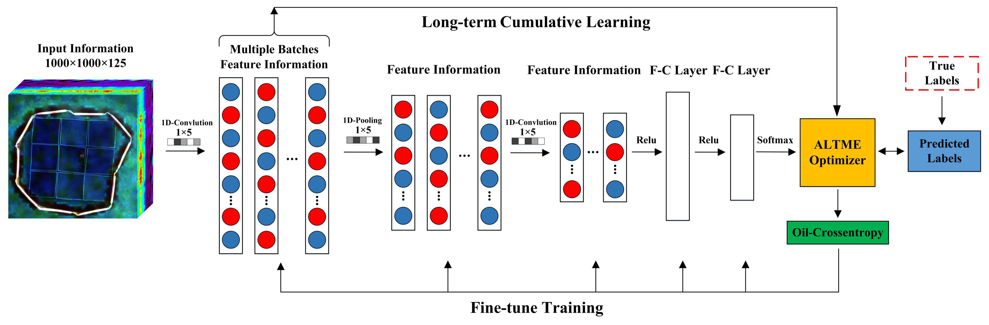
The oil-spill data of the experiment were obtained using the UAV’s hyperspectral sensor. Moreover, the data are 1000 × 1000 × 125 pixels in size and have the characteristics of a high number of spectral dimensions and rich information. To ensure computational efficiency and training performance, the training of the deep learning models was carried out in multiple batches and over different periods.

ALTME improves the gradient update mechanism of the second momentum item and assigns an adaptive cumulative learning weight to the oil-spill spectral characteristic information of multiple batches and different periods. The adaptive selection of the second momentum item weight is realized through an iterative process, and the proportion of long-term accumulated spectral information learning is increased under the premise of ensuring model convergence. Deep learning experiments using the ALTME optimizer can theoretically enable the model to remember the long-term spectral characteristic information of different batches, allowing it to perform better and more smoothly during the iterative training; thus, improving the accuracy and stability of its oil-spill detection ability. In addition, we use a momentum correction term for the ALTME optimizer, which can effectively avoid instability in the first and second momentum terms due to the small gradient in the early stage of training, which will affect the model training.

The algorithm of the ALTME optimizer is shown in Algorithm 1, where β represents the first moment, λ is the adaptive cumulative learning weight, iter is the number of iterations, g_t represents the gradient at time t, m_t is the first momentum term, v_t represents the second momentum term, m_t^correct represents the first momentum correction term, v_t^correct is the second momentum correction term, Loss(·) represents the loss function, θ_t is the weight of the deep learning model, α represents the learning rate, and ε is the weight correction value.

Algorithm 1 Adaptive Long-term Moment Estimation

1: Input: β = 0.9, λ ∈ [ 1×10−4, 1×10−5 ] 2: Initialize iter = 0, m0 = 0, v0 = 0 3: for λ = 1×10−4 to 1×10−5 do 4: Repeat 5:   for t = 1 to T do 6:      gt = ▽θ Loss( θt ) 7:      mt = βmt-1 + ( 1 - β )gt 8:      vt = ( 1 + λ )vt-1 + λgt2 9:      mtcorrect = mt / ( 1 - βt ) 10:     vtcorrect = vt / (( 1 + λ )t - 1 ) 11:     θt = θt-1 - α·mtcorrect / ( $\sqrt{v_t{}^{\mathrm{correct}}}$ + ε ) 12:   End for 13:  iter ← iter + 1 14: End for

We derive the gradient update process of the second momentum correction term v_t^correct of the ALTME optimizers as follows.

$$\begin{array}{l}{v}_t^{\mathrm{correct}}=\frac{v_t}{{\left(\lambda +1\right)}^t-1}\\ =\frac{\left(\lambda +1\right)v_{t-1}+\lambda g_t^2}{{\left(\lambda +1\right)}^t-1}\\ =\frac{\left(\lambda +1\right)·\left[{\left(\lambda +1\right)}^{t-1}-1\right]v_{t-1}^{\mathrm{correct}}+\lambda g_t^2}{{\left(\lambda +1\right)}^t-1}\\ =\frac{{\left(\lambda +1\right)}^t-\lambda -1}{{\left(\lambda +1\right)}^t-1}{v}_{t-1}^{\mathrm{correct}}+\frac{\lambda }{{\left(\lambda +1\right)}^t-1}{g}_t^2\\ =\left[1-\frac{\lambda }{{\left(\lambda +1\right)}^t-1}\right]v_{t-1}^{\mathrm{correct}}+\frac{\lambda }{{\left(\lambda +1\right)}^t-1}{g}_t^2\\ \end{array}$$

(3)

We replace $1-\frac{\lambda }{{\left(\lambda +1\right)}^t-1}$ with φ, and the gradient updating process of the second momentum correction term becomes

$$v_t^{\mathrm{correct}}=\phi v_{t-1}^{\mathrm{correct}}+\left(1-\phi \right)g_t^2$$

(4)

The ALTME optimizer still updates the gradient based on the mechanism of exponential moving average. When t→∞, φ→1, and the learning rate will approach a constant. The second momentum term will update the model weights more smoothly with a smaller correction force so that the ALTME optimizer can not only learn the long-term spectral characteristic gradients of different training batches but also maintain better stability during the training and convergence stages.

2.3. Marine Oil-Spill Detection 1D-CNN Model

The aim of the proposed ALTME optimizer is to meet the needs of marine oil-spill detection based on hyperspectral remote sensing by conforming to the characteristics of experimental data and adapting to different oil-spill scenarios. Hence, by assigning an adaptive weight to the long-term spectral characteristic information of oil spills, we increase the cumulative learning proportion of the spectra of different batches to avoid the loss of effective spectral characteristic information.

Because the target of this detection research is an oil spill in an experimental enclosure, it has no obvious spatial characteristics. Therefore, the ALTME optimizer is implemented in a 1D-CNN, which is more suitable for extracting features from 1D spectral information to build the oil-spill detection model. Using this model, we extract the spectral characteristic data of the oil-spill hyperspectral images, construct the mapping relationship between spectral characteristic data and the sample labels, and then identify the type of oil spills and detect oil films with different thicknesses. The model structure is shown in Figure 9.

In contrast to traditional convolution, the convolution in a 1D-CNN has a receptive field based on a 1D plane convolution kernel, which has a strong feature extraction ability and can fit nonlinear data well. Because of the sparse representation and weight sharing, the number of parameters of the marine oil-spill detection model is greatly reduced, and the efficiency of detection is improved. The calculation is as follows.

$$h_{i,j}=g\left[{\displaystyle \sum }_m^M\left(h_{i-1,m}\times w_{i,mj}\right)+b_{i,j}\right]$$

(5)

Here, h_i,j represents the jth output feature map of the ith convolution layer, M is the number of feature maps of the ith convolution layer, w_i,mj represents the weight, b_i,j is the bias, and g(f) represents the activation function.

In the model proposed in this paper, the rectified linear unit (ReLU) function is chosen as the activation function. The function enables the model to perform gradient descent more efficiently while maintaining a fast calculation speed and can avoid the phenomena of gradient disappearance and expansion. The formula of the ReLU function is

$$g\left(x\right)=\max \left(0,x\right)$$

(6)

We set the pooling method of the detection model to 1D maximum pooling, which can reduce the risk of overfitting and enhance the robustness of the model through the pooling process. Each pooling layer corresponds to the receptive field of the convolutional layer of size N × 1. The maximum pooling formula is as follows.

$${\mathrm{a}}_j=\underset{N\times 1}{\max }\left({\mathrm{a}}_i^{n\times 1}u\left(n,1\right)\right)$$

(7)

Here, max() represents the 1D maximum pooling function, u(n, 1) is the window function of the convolution layer, and a_j is the maximum value in the neighborhood.

Since the research is oriented to the detection of multiple oil spill targets, multi-classification cross entropy is selected as the loss function to carry out oil spill detection based on a softmax classifier. The oil-crossentropy function is as follows.

$$\mathrm{oil}-\mathrm{crossentropy}=-\left[{\displaystyle \sum }_{i=1}^n{P}_i·\log \left(\frac{e^{Z_i}}{Z}\right)\right],Z={\displaystyle \sum }_{i=1}^n{e}^{z_i}$$

(8)

Here, Z_i is the logits function of the softmax classifier, n is the number of detection targets, P_i is the true sample distribution.

The reverse fine-tuning process of the oil-spill detection model uses the backpropagation algorithm combined with the calibrated label data to adjust the weight and parameters of the model layer by layer so that the model can optimize the mapping of the oil-spill spectral characteristic data.

The structure of the proposed model, which is based on a Keras and TensorFlow framework, is shown in

Table 4. Structure of the marine oil spill detection 1D-CNN model.

Layer	Number	Kernel	Stride
Convolutional layer-1	150	1 × 5	1
MaxPooling layer-1	-	1 × 5	3
Convolutional layer-2	100	1 × 5	1
MaxPooling layer-2	-	1 × 5	3
Convolutional layer-3	50	1 × 5	1
MaxPooling layer-3	-	1 × 5	1
Fully connected layer-1	200	-	-
Fully connected layer-2	100	-	-

. The model consists of three 1D convolutional layers, three 1D maximum pooling layers, and two fully connected layers. Through iterative training and hyperparameter tuning, the model acquires the ability to identify oil-spill types and detect oil films with different thicknesses.

2.4. Accuracy Evaluation Indexes

The overall accuracy (OA) and Kappa coefficient were respectively chosen to measure the overall detection performance and consistency of the oil-spill detection results. Because the seawater pixels in the oil-spill hyperspectral images account for a large proportion of the image and have a greater impact on OA, the OA alone cannot effectively reflect the detection accuracy of each experimental group. By contrast, the F₁-score takes into account both recall and precision, which removes the imbalance between the two metrics. Therefore, the F₁-score was selected to measure the single-target detection accuracy of the proposed model for each experimental group. The calculation formulas of each accuracy evaluation index are as follows:

$$\mathrm{Recall}=\frac{\mathrm{TP}}{\mathrm{TP}+\mathrm{FN}}\times 100\%$$

(9)

$$\mathrm{Precision}=\frac{\mathrm{TP}}{\mathrm{TP}+\mathrm{FP}}\times 100\%$$

(10)

$$F_1-\mathrm{score}=2·\frac{\mathrm{Recall}·\mathrm{Precision}}{\mathrm{Recall}+\mathrm{Precision}}$$

(11)

$$\mathrm{OA}=\frac{\mathrm{TP}+\mathrm{TN}}{\mathrm{TN}+\mathrm{TP}+\mathrm{FN}+\mathrm{FP}}\times 100\%$$

(12)

$$\mathrm{Kappa}=\frac{\mathrm{TP}+\mathrm{TN}}{\left(\mathrm{TN}+\mathrm{FP}\right)·\left(\mathrm{TN}+\mathrm{FN}\right)·\left(\mathrm{FN}+\mathrm{TP}\right)·\left(\mathrm{FP}+\mathrm{TP}\right)}$$

(13)

where TP represents the number of true positives, TN is the number of true negatives, FP represents the number of false positives, and FN is the number of false negatives.

3. Results and Discussion

3.1. Analysis of Oil-Spill Spectrum Characteristics

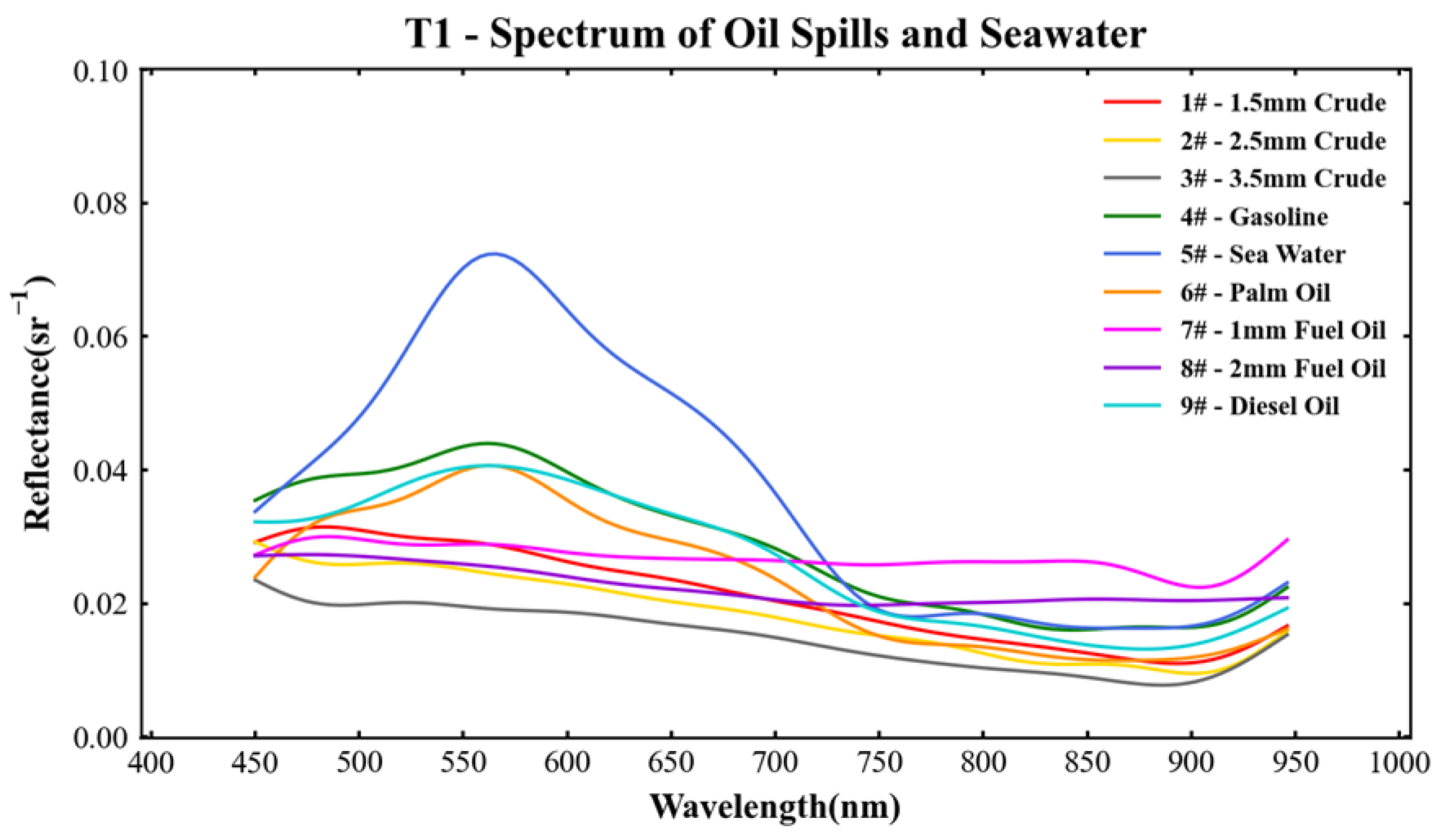
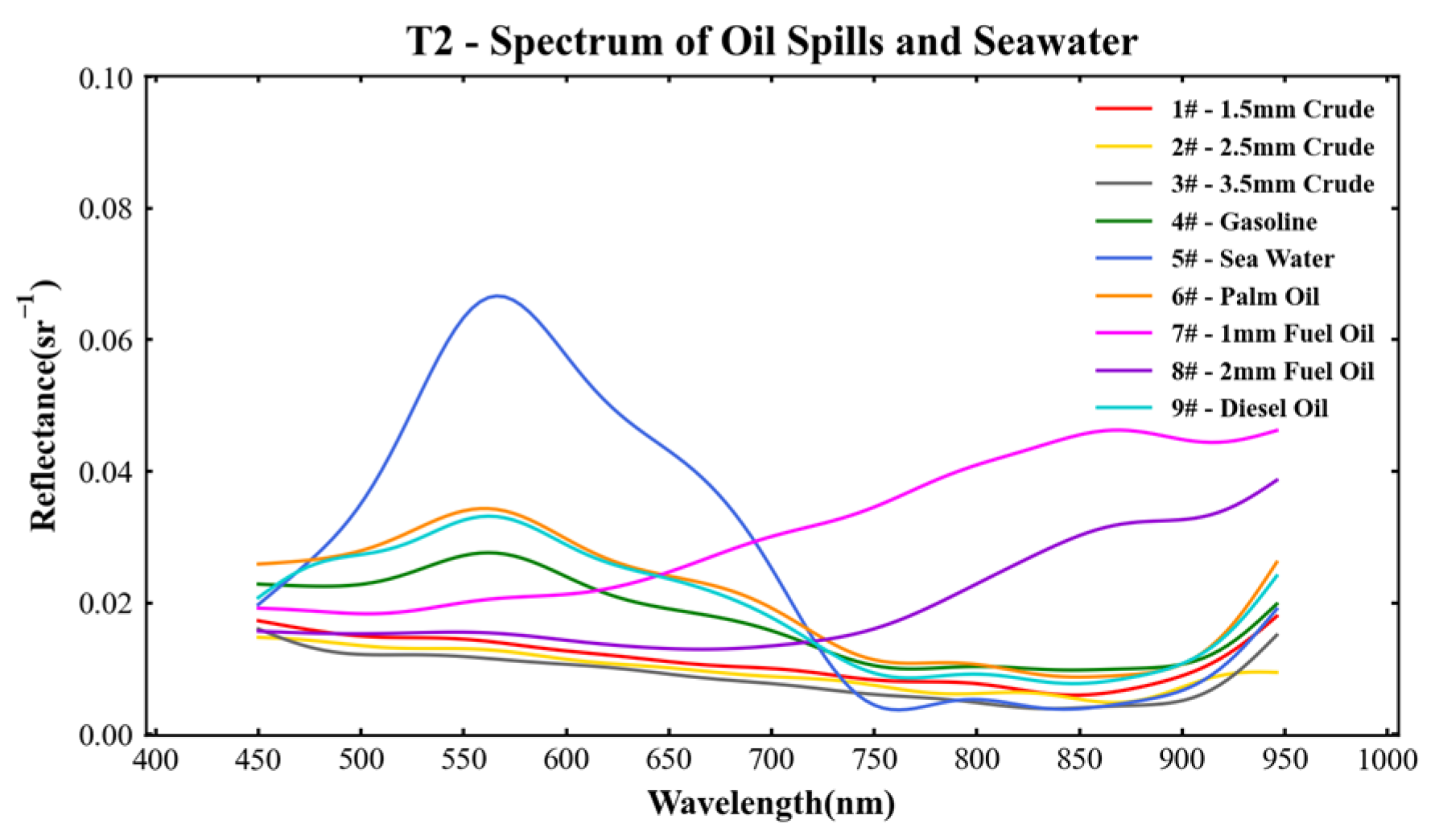
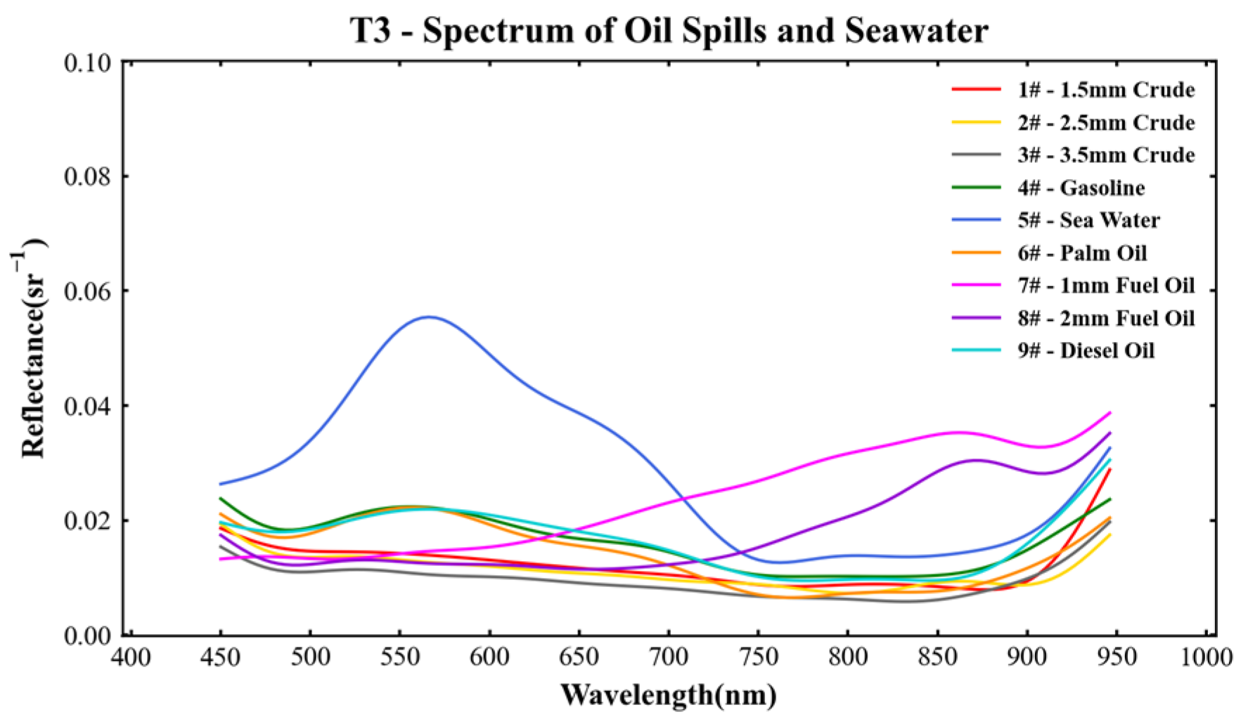
We averaged and smoothed the hyperspectral data of the oil spill and seawater experimental groups. The remote sensing reflectance hyperspectral curves of the experimental groups at T1–T3 are shown in Figure 10, Figure 11 and Figure 12, respectively.

3.1.1. Seawater and Light-Oil Experimental Groups at T1

The remote sensing reflectance of the seawater (group 5) is higher than all the oil-spill groups in the visible light range of 450–720 nm. In the near-infrared range beyond 760 nm, the reflectance decreases because of the absorption characteristics of seawater. Because of the chlorophyll in the water, the hyperspectral curve of seawater has a peak at the 560 nm green light band. The reflectance trends of the three light-oil experimental groups of gasoline (group 4), palm oil (group 6), and diesel (group 9) are similar, and the overall reflectance is lower than that of seawater. Because of the high transmittance of light oils, the three groups of light oils are strongly affected by the background water body, and the spectral curves all have small peaks around 560 nm. In addition, the reflectances of the three light-oil experimental groups are not very separable in the whole band, and there is little information that could be extracted and poor potential for type recognition.

3.1.2. Crude Oil Experimental Groups at T1

The spectral curves of the crude oil (groups 1–3) with different thicknesses are spectrally separable in the visible and near-infrared bands of 450–900 nm. The overall spectrum shows a downward trend, and the overall reflectance is inversely proportional to the oil film thickness, which is consistent with Liu and Sun’s research conclusion [46,47]. We believe that this is related to the strong absorption characteristics of crude oil. The thicker the oil film, the stronger the absorption capacity of sunlight, which decreases the reflectance. The reflectance of these groups tends to increase in the near-infrared bands of 900-950 nm, which is related to the backscattering properties of crude oil.

3.1.3. Fuel Oil Experimental Groups at T1

The remote sensing reflectance curves of the fuel oil (groups 7 and 8) with different thicknesses tend to be relatively gentle over the whole waveband, and there is spectral separability information that can be extracted. The overall reflectance is inversely proportional to the oil film thickness. Moreover, the overall reflectance of the 1-mm thick fuel oil (group 7) is higher than that of the 2-mm thick fuel oil (group 8). The oil film spectrum curve of group 7 dips at 910 nm. Because of the backscattering effect of fuel oil, the curves of these groups tend to increase after 910 nm.

3.1.4. Seawater and Light-Oil Experimental Groups at T2–T3

As time passes, the solar elevation angle decreases, the sunlight intensity weakens, and the overall remote sensing reflectance of the seawater (group 5) gradually decreases. The reflectance of the seawater is still affected by the chlorophyll at T2–T3, so the reflection peak appears at 560 nm, and the reflectance decreases in the near-infrared bands. The reflectance of the three light-oil experimental groups is affected by the background water body, and there is still a reflection peak at 560 nm, but with the passage of time, this peak gradually decreases. In addition, as sunlight intensity decreases, the spectral separability of the light-oil groups further decreases. In particular, at T3, the reflectance of the light-oil groups has only a weak spectral separability in the visible light bands.

3.1.5. Crude Oil Experimental Groups at T2–T3

Because the sunlight intensity has decreased, the separability of the spectral curves of the crude oil with different thicknesses (groups 1–3) in the range of 450–900 nm is lower than that at T1. However, the overall remote sensing reflectance still retains the overall inverse proportionality with respect to the oil film thickness; that is, a thicker oil film thickness leads to a lower overall reflectance. The reflectances of the crude oil in groups 1–3 tend to increase in the near-infrared bands of 900–950 nm, which is more obvious than at T1. We believe that over time, crude oil and seawater may undergo partial emulsification, causing the reflectance of these groups to increase in the near-infrared bands.

3.1.6. Fuel Oil Experimental Groups at T2–T3

The reflectance curves of the fuel oil (groups 7 and 8) change substantially when compared with the results from T1. Moreover, the spectral response begins to appear in the visible light bands, and the overall waveband tends to increase. We believe this phenomenon is caused by the emulsification reactions of fuel oil and seawater. In addition, groups 7 and 8 still have spectral separability, the overall reflectance is inversely proportional to the oil film thickness, and both experimental groups have spectral troughs at the 910-nm band.

In summary, the spectral curves of the light-oil experimental groups are similar, and the spectral separability is weak. As time passes from T1 to T3, the sunlight intensity weakens and the spectral separability further decreases, and only a weak spectral difference exists at T3. Moreover, there are certain spectral differences between the groups of heavy oil with different thicknesses, and the spectral separability decreases as sunlight intensity decreases. When sunlight intensity is low, it may be difficult to accurately distinguish the type of light oil and detect the thickness of heavy oils based on traditional remote sensing methods. Therefore, we apply deep learning techniques to the actual measured hyperspectral oil-spill data to effectively extract the characteristic information of oil-spill spectral curves to accurately identify the type of oil spills and detect the thickness of the thick oil films.

3.2. Selection and Analysis of Basic Oil-Spill Detection Models

Because this detection experiment is for 1D oil-spill spectral information, we built representative SVM, GRU, and 1D-CNN oil-spill detection models using Keras and TensorFlow, which are widely used in 1D signal recognition. We used the oil-spill UAV hyperspectral data and compared and analyzed the detection results obtained by different models at different times and phases, and selected the best basic marine oil-spill detection model. All experiments were performed on a Dell Precision 7820 Tower Workstation equipped with a Xeon-Gold 5122 processor and an NVIDIA-RTX2080Ti graphics processing unit. Each group of oil-spill detection experiments was carried out five times, and the reported detection accuracy is the average value of the five experiments, as shown in

Table 5. Accuracy of the detection results at T1.

	Index
Model	SVM			GRU			1D-CNN
Group	Recall	Precision	F1-Score	Recall	Precision	F1-Score	Recall	Precision	F1-Score
1#-1.5 mm Crude	85.93	83.88	0.849	90.07	95.98	0.929	98.75	96.42	0.976
2#-2.5 mm Crude	78.95	79.33	0.791	93.98	89.84	0.919	97.40	97.73	0.976
3#-3.5 mm Crude	85.84	83.08	0.844	93.41	95.52	0.945	97.05	98.07	0.976
4#-Gasoline	87.45	86.89	0.872	92.80	89.84	0.913	98.55	97.62	0.981
5#-Seawater	96.82	95.57	0.962	97.75	97.82	0.978	98.48	98.63	0.986
6#-Palm Oil	84.65	87.21	0.859	95.43	91.79	0.936	99.03	95.31	0.971
7#-1 mm Fuel Oil	93.48	89.47	0.914	98.32	97.48	0.979	98.27	98.56	0.984
8#-2 mm Fuel Oil	90.26	95.47	0.928	95.56	97.79	0.967	98.52	97.02	0.978
9#-Diesel Oil	82.14	92.21	0.869	94.61	92.34	0.935	98.16	97.45	0.978
10#-PVC	79.40	86.76	0.829	82.55	88.88	0.856	85.52	89.13	0.873
11#-Oil Boom	92.8	94.93	0.939	95.58	94.51	0.951	93.51	96.39	0.949
OA (%)	92.34			95.97			97.76
Kappa	0.882			0.939			0.966
Time (min)	19.12			4.79			11.68

,

Table 6. Accuracy of the detection results at T2.

	Index
Model	SVM			GRU			1D-CNN
Group	Recall	Precision	F1-Score	Recall	Precision	F1-Score	Recall	Precision	F1-Score
1#-1.5 mm Crude	71.92	80.13	0.758	85.12	89.73	0.874	95.66	98.05	0.968
2#-2.5 mm Crude	85.77	76.07	0.806	97.23	88.65	0.927	98.55	95.76	0.971
3#-3.5 mm Crude	66.77	82.21	0.737	83.45	89.70	0.865	96.00	97.23	0.966
4#-Gasoline	80.36	78.95	0.797	92.40	88.65	0.905	97.56	96.30	0.969
5#-Seawater	97.68	94.80	0.962	97.56	97.61	0.976	98.30	98.62	0.985
6#-Palm Oil	83.90	81.74	0.828	95.96	87.08	0.913	98.72	93.24	0.959
7#-1 mm Fuel Oil	97.06	97.10	0.971	98.41	97.60	0.980	98.28	98.84	0.986
8#-2 mm Fuel Oil	96.66	96.69	0.967	97.79	97.37	0.976	98.92	98.32	0.986
9#-Diesel Oil	71.93	87.68	0.790	88.48	93.74	0.910	97.80	94.46	0.961
10#-PVC	76.00	92.73	0.835	80.99	90.31	0.854	83.08	91.09	0.869
11#-Oil Boom	94.84	95.93	0.954	96.14	95.92	0.960	96.27	95.56	0.959
OA (%)	91.76			95.31			97.53
Kappa	0.869			0.927			0.961
Time (min)	18.15			4.95			11.77

and

Table 7. Accuracy of the detection results at T3.

	Index
Model	SVM			GRU			1D-CNN
Group	Recall	Precision	F1-Score	Recall	Precision	F1-Score	Recall	Precision	F1-Score
1#-1.5 mm Crude	74.79	79.05	0.769	88.38	94.64	0.914	98.40	96.44	0.974
2#-2.5 mm Crude	79.48	65.54	0.718	92.05	87.19	0.896	98.37	96.09	0.972
3#-3.5 mm Crude	53.16	76.10	0.626	81.36	87.59	0.844	95.10	97.36	0.962
4#-Gasoline	71.69	70.41	0.710	91.74	88.54	0.901	96.76	95.94	0.964
5#-Seawater	97.79	93.95	0.958	97.75	97.15	0.975	98.52	98.36	0.984
6#-Palm Oil	74.03	78.47	0.762	95.57	88.74	0.920	98.26	94.86	0.965
7#-1 mm Fuel Oil	95.60	96.17	0.959	97.59	96.24	0.969	98.34	97.75	0.981
8#-2 mm Fuel Oil	91.79	95.20	0.935	95.36	96.67	0.960	98.52	96.96	0.977
9#-Diesel Oil	58.73	66.98	0.626	89.78	86.85	0.883	96.90	94.00	0.954
10#-PVC	67.24	95.08	0.788	71.85	93.22	0.812	73.94	93.22	0.825
11#-Oil Boom	95.57	96.55	0.961	97.07	95.48	0.963	96.89	95.38	0.961
OA (%)	89.23			94.84			97.32
Kappa	0.829			0.920			0.958
Time (min)	17.08			4.88			11.73

.

As Table 5 shows, in the oil-spill detection experiment at time T1, the OA of the 1D-CNN model reaches 97.76%, and the Kappa coefficient reaches 0.966, both of which are higher than the detection accuracies of the SVM and GRU models. The 1D-CNN model has higher detection accuracy F₁-scores for the seawater (group 5), oil spills (groups 1–4 and 6–9), and PVC enclosure (group 10) than the SVM and GRU models. The recognition accuracy F₁-score for light-oil types is more than 0.971, and the detection accuracy for heavy oils with different thicknesses is more than 0.976. The GRU model is more sensitive to the detection of the oil containment boom (group 11), and its F₁-score reaches 0.951, which is better than the scores of the other two detection models. In addition, the calculation speed of the GRU model is much higher than that of the SVM and 1D-CNN models; its oil-spill detection process only takes 4.79 min.

The results in Table 6 show that in the oil-spill detection experiment at T2, the 1D-CNN model performs well, with an OA of 97.53% and a Kappa coefficient of 0.961, both of which are higher than the SVM and GRU models. The F₁-scores of the 1D-CNN model for the seawater (group 5), the oil spill (groups 1–4 and 6–9), and the enclosure (group 10) are overall higher than those of the SVM and GRU models. The recognition accuracy F₁-score for light-oil types is larger than 0.959, and the detection accuracy for heavy-oil groups with different thicknesses is larger than 0.966. The detection accuracy F₁-score of the GRU model for the oil containment boom (group 11) is 0.960, which is higher than the scores of the other two models, indicating that this model retains excellent detection performance.

It can be seen from Table 7 that in the detection experiment at T3, the OA of the 1D-CNN reaches 97.32%, and the Kappa coefficient reaches 0.958, both of which are higher than the scores of the other two types of detection models. The 1D-CNN model has a higher detection accuracy F₁-score for all single targets except the oil containment boom (group 11), but its detection speed is slower, taking 11.73 min. The detection accuracy F₁-score for heavy oils with different thicknesses is larger than 0.962, and the recognition accuracy for light-oil types is larger than 0.954. The GRU model still detects the oil containment boom (group 11) best, with an F₁-score of 0.963. In addition, the GRU model still detects oil spills very efficiently, taking only 4.88 min, which is much faster than the other two models.

As shown in Figure 13, in the detection results of the SVM model at time T1, there are obvious misclassifications in several experimental groups. Moreover, the SVM detection model has a generally poor detection performance for the experimental groups of heavy oils with different thicknesses, and there is much room for improvement in the identification of light oils. The detection result of the GRU model at T1 is better than that of SVM, and the detection performance of the fuel oil (groups 7 and 8) is improved, but there is a partial misclassification in the 3.5-mm thick crude oil (group 3) and the seawater (group 5). Compared with the other two types of oil-spill detection models, the 1D-CNN model has a better overall detection performance, but the problem of misclassification in the 3.5-mm thick crude oil (group 3) and the fuel oil (groups 7 and 8) has not been completely resolved.

At T2, the detection results of the SVM and GRU models for the fuel oil (groups 7 and 8) are acceptable. However, their detection performance for crude oil (groups 1–3), gasoline (group 4), seawater (group 5), and diesel oil (group 9) are poor. These models fail to complete the tasks of detecting the thickness of the heavy-oil film and identifying the type of oil spill, and neither of them could effectively detect the oil containment boom of the diesel experiment (group 9). Compared with the other two models, the detection performance of the 1D-CNN model at time T2 is much better, but there is still room for improvement in the identification of the enclosures for the gasoline (group 5) and diesel (group 9).

At T3, the SVM and GRU oil-spill detection models have more difficulty than they did at T1 and T2, and they cannot effectively extract the differences between the oil-spill spectra and hence cannot identify the type of oil spills and detect the thickness of the oil films. The detection result of the 1D-CNN model at T3 is better than those of the other two models, but the overall detection performance is worse than it is at T1 and T2. The recognition results of the model on the enclosures of the 3.5-mm thick crude oil (group 3), gasoline (group 5), 2-mm thick fuel oil (group 8), and diesel (group 9) still need to be improved.

In summary, the OA and Kappa coefficients of the 1D-CNN oil-spill detection model at T1–T3 are higher than those of the SVM and GRU models, and its single target detection accuracy F₁-scores for different oil-spill experimental groups are all higher than the other two detection models. From the perspective of detection performance, at each observation point, the 1D-CNN model is better than the SVM and GRU oil-spill detection models. The advantage of the GRU model is that the model converges quickly and can accurately identify the oil containment boom. Moreover, the oil-spill detection process only takes about 4 min. In the future, it could be used for rapid emergency detection in large-scale marine oil-spill disasters. Under the same experimental conditions, the detection time of the 1D-CNN model is about 12 min, but the detection accuracy and performance of this model are much better than those of the GRU model, and the calculation efficiency is within an acceptable range for this experiment.

In addition, we found that the detection performance of the same oil-spill detection model at different moments deteriorates over time, and the detection performances of the models at T3 are substantially worse than they are at T1 and T2. We believe that this is related to the solar elevation angle, which decreases over time in this experiment, and the sunlight intensity, which correspondingly decreases. It is not difficult to see in Figure 10, Figure 11 and Figure 12 that, from T1 to T3, as the sunlight intensity gradually decreases, the spectral separability between different types of light oils and heavy oils with different thicknesses weakens. Hence, the detection performance of an oil-spill detection model decreases over time. The experimental results show that the reduction in sunlight intensity reduces the spectral separability of the oil-spill experimental groups, which has a substantial impact on the SVM and GRU models, whereas the 1D-CNN model yields relatively stable detection capabilities. In this study, based on the detection accuracy, performance, and single-target accuracy of the three oil-spill detection models at different times, the 1D-CNN model was selected as the basic oil-spill detection model.

3.3. Adaptive Selection and Analysis of the Cumulative Learning Weight of the ALTME Optimizer

The ALTME optimizer assigns adaptive cumulative learning weights to the long-term spectral information of experimental hyperspectral data, making full use of the oil-spill spectral information and achieving the purpose of cumulatively learning the spectral characteristic information of different batches. We have determined through experiments that the adaptive range of the cumulative learning weight λ of the model under the premise of stable convergence is 1 × 10⁻⁴–5 × 10⁻⁴. We then used iterative experiments to realize the adaptive selection process of the cumulative learning weight. The optimizer considers the OA and Kappa coefficients, compares the F₁-score of different oil-spill groups, and extracts the spectral cumulative learning weights that best fit the oil-spill experiment scene at different times. The ALTME optimizer was then constructed using the selected cumulative learning weight, which was integrated with the 1D-CNN to build the marine oil-spill detection 1D-CNN model for identifying the type of oil spills and detecting heavy-oil films with different thicknesses. As shown in

Table 8. Accuracy of the adaptive selection of the cumulative learning weight at T1-T3.

	Index
Moment	T1			T2			T3
λ	3 × 10−4			3 × 10−4			2 × 10−4
Group	Recall	Precision	F1-Score	Recall	Precision	F1-Score	Recall	Precision	F1-Score
1#-1.5 mm Crude	99.42	99.53	0.995	99.28	99.54	0.994	99.14	97.59	0.984
2#-2.5 mm Crude	99.56	99.08	0.993	99.63	98.67	0.991	98.91	97.78	0.983
3#-3.5 mm Crude	99.49	98.85	0.992	99.58	98.13	0.989	98.29	97.69	0.980
4#-Gasoline	99.46	99.19	0.993	99.44	98.61	0.990	98.82	97.44	0.981
5#-Seawater	99.42	99.31	0.994	99.32	99.27	0.993	98.89	98.90	0.989
6#-Palm Oil	99.67	99.11	0.994	99.85	97.92	0.989	98.52	98.38	0.985
7#-1 mm Fuel Oil	99.66	99.30	0.995	99.74	99.39	0.996	98.78	98.65	0.987
8#-2 mm Fuel Oil	99.69	98.67	0.992	99.65	99.38	0.995	99.35	97.52	0.984
9#-Diesel Oil	99.40	98.99	0.992	99.50	98.66	0.991	98.88	95.56	0.972
10#-PVC	86.84	92.52	0.896	87.04	93.32	0.901	77.93	92.13	0.844
11#-Oil Boom	96.80	97.62	0.972	96.37	97.90	0.971	97.11	95.75	0.964
OA (%)	98.96			98.35			98.09
Kappa	0.984			0.974			0.970
Time (min)	12.15			12.22			12.07

, at T1–T3, the adaptive cumulative learning weight λ of the ALTME optimizer has values of 3 × 10⁻⁴, 3 × 10⁻⁴, and 2 × 10⁻⁴, respectively.

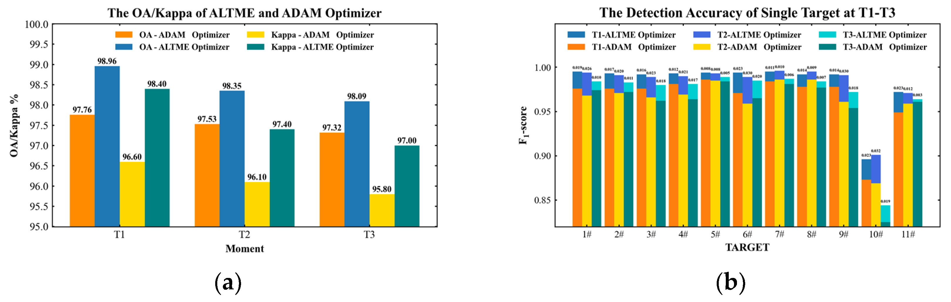
As Table 8 shows, the OA and Kappa coefficients of the marine oil-spill detection model at T1 are higher than those at T2 and T3, and the accuracy of detection for all single targets except for fuel oil (groups 7 and 8) is also higher. The recognition accuracy F₁-score for light-oil types is larger than 0.972, and the detection accuracy for heavy oils is larger than 0.980. Experimental results show that although the oil-spill detection model has strong feature extraction capabilities, it is limited by the low spectral difference of the oil-spill spectral data at T2 and T3, which will affect detection accuracy to a certain extent. It can be seen from Figure 14 that after the oil-spill detection model has been equipped with the ALTME optimizer, the detection capability is fully enhanced at T1–T3, and the OA, Kappa, and single detection accuracy F₁-score values have all been improved to varying degrees.

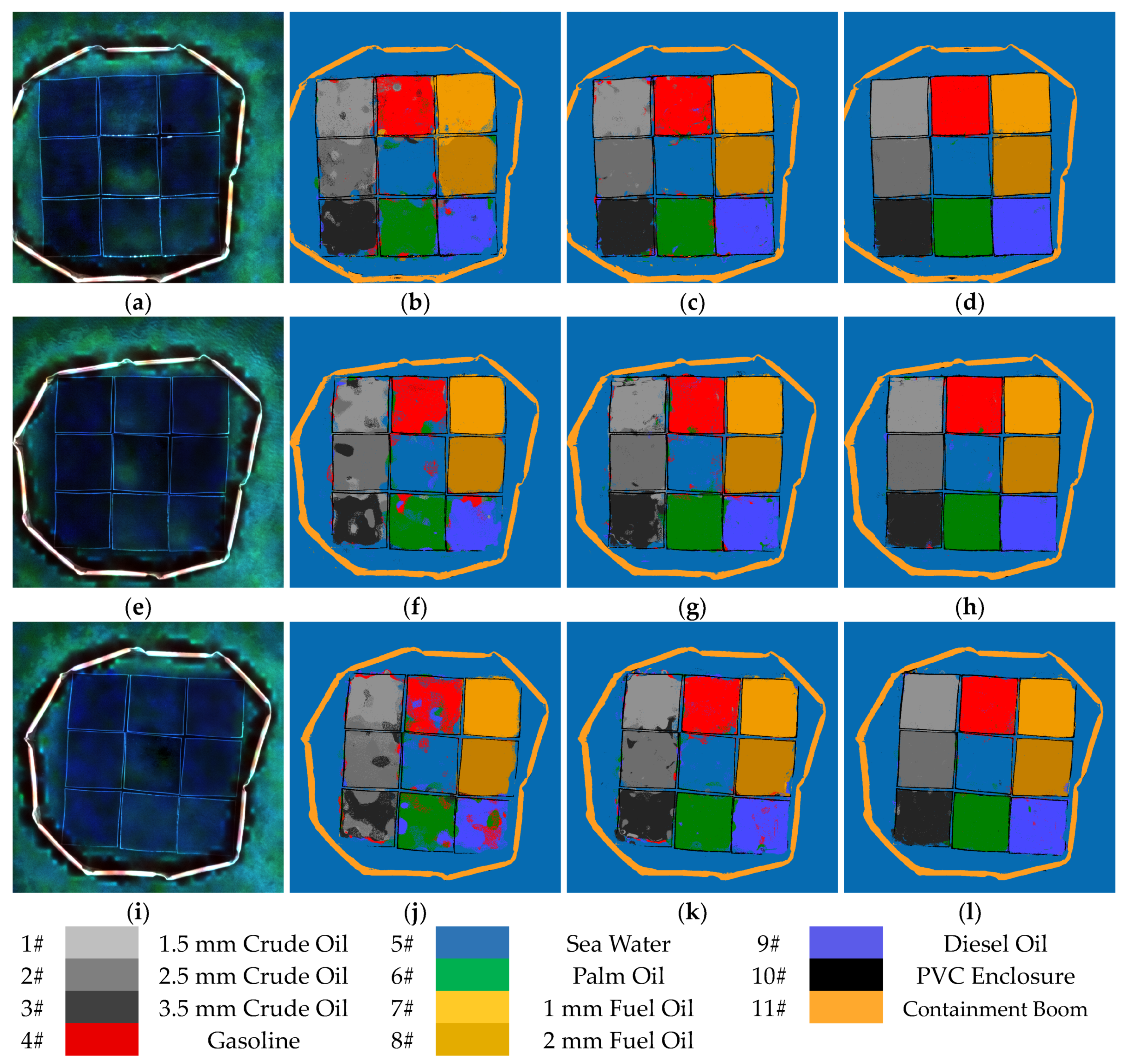
It can be seen from Figure 15 that at T1, the marine oil-spill detection model equipped with the ALTME optimizer can accurately identify the type of oil spills and detect different thicknesses of thick oil films, correcting the obvious misclassifications of the basic oil-spill detection 1D-CNN model for 3.5-mm thick crude oil (group 3) and fuel oil (groups 7 and 8). At T2, the proposed detection model improves the detection ability of the basic model for the 3.5-mm thick crude oil (group 3) and improves the identification performance of gasoline (group 5) and diesel (group 9). At T3, the proposed detection model counters the influence of poor data spectral separability. By cumulatively learning long-term oil-spill spectral characteristic information, the problem of misclassifications of the experimental enclosure is effectively solved, and the overall oil-spill detection results are improved.

3.4. Analysis of the Stability and Applicability of the ALTME Optimizer

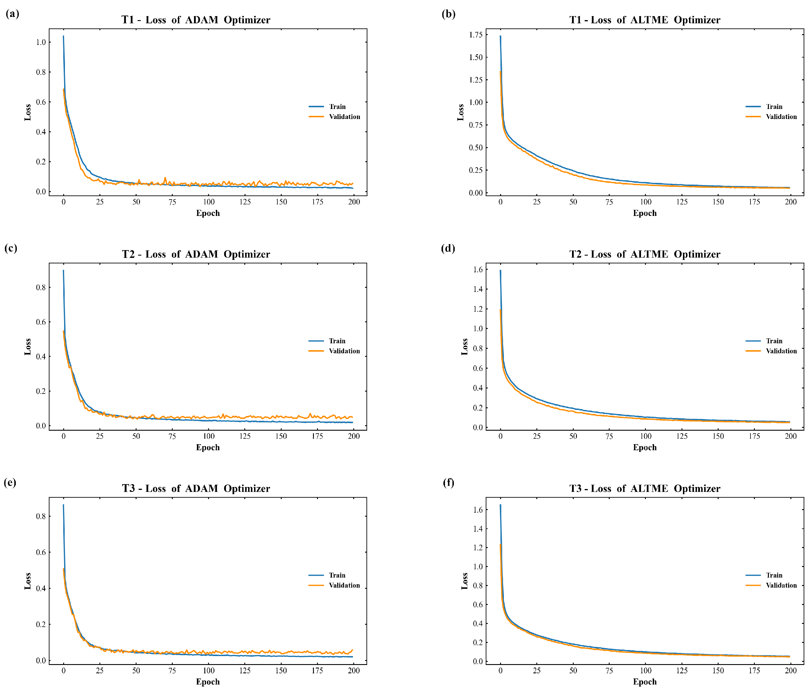
In this study, the stability of the optimizer was analyzed by comparing the decreases in loss value of the ALTME and Adam optimizers during the training process. As shown in Figure 16, in contrast to the parameter update process of the Adam optimizer of the traditional 1D-CNN model, the parameter update process of ALTME has an update mechanism based on the second momentum term of the optimizer, and the oil-spill detection model that uses the ALTME optimizer will accumulate and learn the long-term spectral characteristic information of different batches. As the number of training iterations increases, the second momentum term of the ALTME optimizer approaches a constant, the magnitude of correction decreases, and the learning rate stabilizes. As a result, the loss of the model decreases steadily during the training process, and the model parameters are updated more smoothly so that the model is more stable at the beginning of the iteration and the convergence stage.

Because of the mechanism of cumulatively learning long-term spectral features in the ALTME optimizer, the amount of calculation may increase and consequently reduce the detection efficiency of the model. In this study, the effect of the ALTME optimizer on detection efficiency was analyzed, and the results are shown in

Table 9. Runtime of the ALTME optimizer cumulative learning weight adaptive selection experiment.

	Time (min)
Optimizer	ADAM	ALTME (λ)
Moment		1 × 10−4	2 × 10−4	3 × 10−4	4 × 10−4	5 × 10−4
T1	11.68	11.97	12.09	12.19	12.29	12.41
T2	11.77	12.01	12.12	12.22	12.35	12.43
T3	11.63	11.93	12.07	12.18	12.27	12.39

. The results reveal that the detection time of the model equipped with the ALTME optimizer instead of Adam increases to varying degrees at T1–T3.

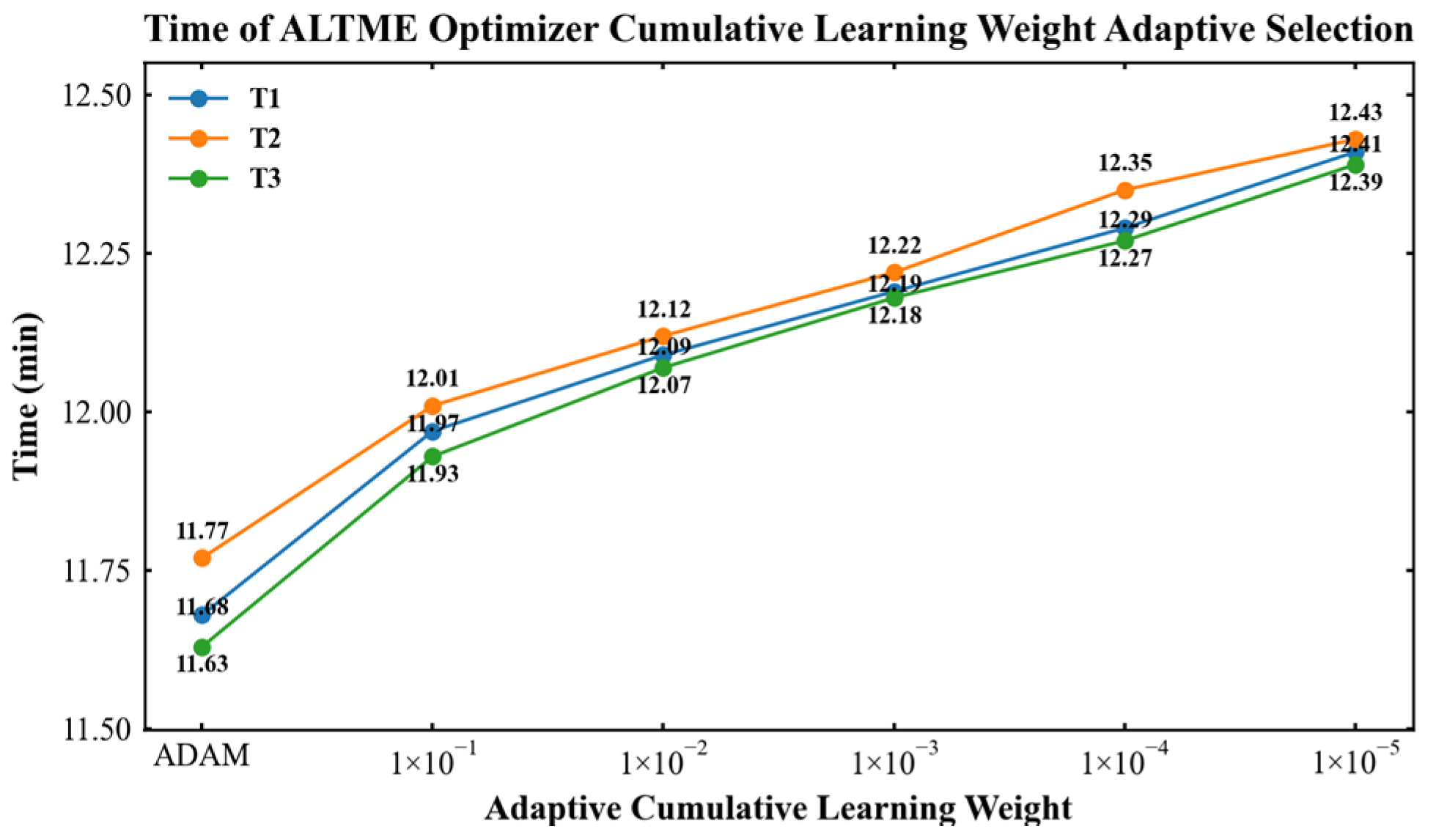
As shown in Figure 17, during the adaptive cumulative weight selection experiment, as the adaptive weight λ gradually increases from 1 × 10⁻⁴ to 5 × 10⁻⁴, the detection time of the model tends to increase. Under the premise of model convergence, as λ increases, the amount of oil-spill spectral information learned by the ALTME optimizer increases, which increases the memory occupied by the model in the graphics processing unit, thereby slowing down the overall convergence process. Because the magnitude of λ in the experiment is only 1 × 10⁻⁴, the update mechanism of the second momentum term of the ALTME optimizer only affects the detection efficiency of the model to a certain extent. The increase in detection time is less than 1 min, which will not incur too much computational burden in the model detection process.

Our experimental data are 1000 × 1000 × 125 pixels in size with a spectral range of 450–950 nm and include nine oil-spill experiment groups. The size of the Pavia University public hyperspectral dataset is 610 × 340 × 103 pixels with a spectral range of 430–860 nm and includes nine types of targets. These specifications are similar to those of the hyperspectral data obtained in our experiment. Therefore, the Pavia University public dataset was selected to verify the applicability of the proposed ALTME optimizer. The number of calibration samples in the Pavia University data is listed in

Table 10. Calibrated sample labels for the Pavia University data.

Group	Class	Samples	Colors
1#	Asphalt	6631
2#	Meadows	18,649
3#	Gravel	2099
4#	Trees	3064
5#	Painted metal sheets	1345
6#	Bare Soil	5029
7#	Bitumen	1330
8#	Self-Blocking Bricks	3682
9#	Shadows	947

. We set the ratio of training samples to test samples to 1:9, which is consistent with the ratio in the oil-spill detection experiment.

As shown in

Table 11. Recognition accuracy results for the Pavia University data.

	Index
Model	SVM			1D-CNN			1D-CNN-ALTME (λ = 2 × 10−4)
Group	Recall	Precision	F1-Score	Recall	Precision	F1-Score	Recall	Precision	F1-Score
1#-Asphalt	93.68	87.44	0.905	92.34	93.79	0.931	94.87	96.47	0.957
2#-Meadows	99.05	90.50	0.946	97.28	93.35	0.953	98.49	98.28	0.984
3#-Gravel	67.72	82.96	0.746	77.14	82.28	0.796	80.38	90.85	0.853
4#-Trees	90.25	96.59	0.933	89.52	94.60	0.920	96.48	97.49	0.970
5#-Painted metal sheets	99.67	99.83	0.998	99.26	97.72	0.985	99.55	99.85	0.997
6#-Bare Soil	68.39	96.33	0.800	79.94	90.32	0.848	95.11	95.22	0.952
7#-Bitumen	48.29	89.20	0.627	87.05	86.54	0.868	91.88	89.99	0.909
8#-Self-Blocking Bricks	89.92	80.65	0.850	88.44	84.78	0.866	93.32	85.69	0.893
9#-Shadows	99.88	100.00	0.999	99.88	99.65	0.998	99.79	100.00	0.999
OA (%)	90.12			91.97			95.91
Kappa	0.866			0.893			0.946
Time (min)	4.46			2.21			2.63

, the adaptive weight λ value of the ALTME optimizer was self-selected to be 2 × 10⁻⁴, which enables the model to cumulatively learn multiple batches of long-term historical spectral feature information to identify the type of targets in the test area. The OA of the 1D-CNN model equipped with the ALTME optimizer is 95.91%, and the Kappa coefficient is 0.946, which are both higher than the results of the SVM and traditional 1D-CNN models. Except for the painted metal sheets (group 5), the detection model with the ALTME optimizer has the best recognition accuracy for the remaining eight types of targets.

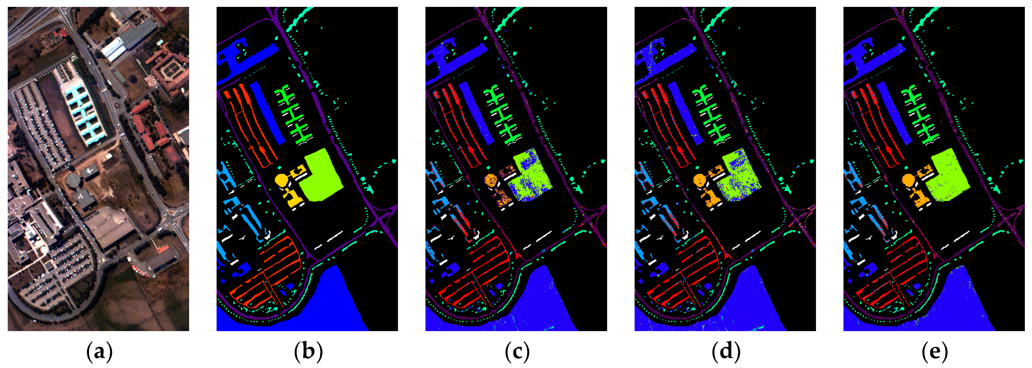
As shown in Figure 18, the recognition results of gravel (group 3) and bitumen (group 7) by SVM and traditional 1D-CNN model are obviously misclassified, and this is even more obvious for bare soil (group 6). The 1D-CNN model with the ALTME optimizer can fully learn the spectral feature information based on the cumulative learning mechanism, effectively improving the recognition performance of various targets in the test area, and the recognition results are more consistent. The airborne hyperspectral remote sensing data used in our oil-spill detection experiment are close to the Pavia University data in terms of data specifications. From this, we conclude that the ALTME optimizer proposed in this paper can improve recognition accuracy by accumulating and learning long-term spectral information, which is suitable for the detection and analysis of hyperspectral remote sensing data. Moreover, it has applicability and generalization ability.

3.5. Feasibility Analysis of Oil-Spill Detection Based on Thermal Infrared Remote Sensing

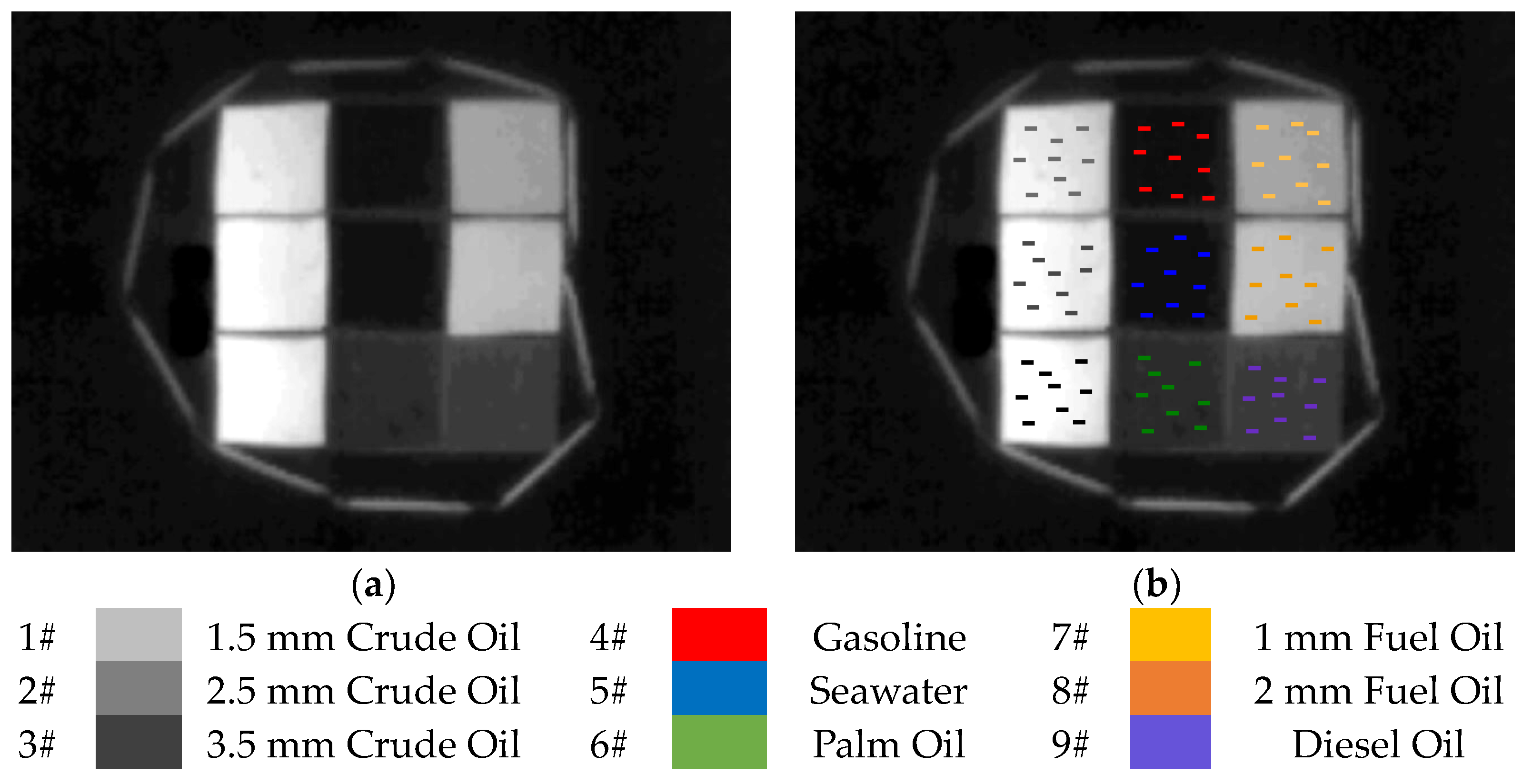
In this study, a feasibility analysis of marine oil-spill detection based on UAV thermal infrared remote sensing technology was also performed. Using the thermal infrared sensor carried by the DJI-Mavic2 drone, a thermal infrared image of oil spills (uncalibrated thermal radiation brightness data) was obtained at 11:20 h. The wavelength range of the sensor is 8–14 µm, and the resolution is 480 × 640 pixels. The low spatial resolution of the thermal infrared image makes it difficult to carry out global sample calibration, so we randomly selected pure samples to conduct the oil-spill thermal infrared detection experiment and verification. Because of the limited endurance of the UAV, only one effective thermal infrared oil-spill image was obtained. The image and sample labels are shown in Figure 19.

The Berrcom JXB-178 (Berrcom, China) infrared thermometer was used to obtain the surface temperature (kinetic temperature) of the oil and seawater at T1–T3, as shown in

Table 12. Temperature information of experimental oil and seawater.

	Temperature (°C)
Group	T1	T2	T3
1#-1.5 mm Crude	44.5	41.6	30.7
2#-2.5 mm Crude	45.2	42.5	30.9
3#-3.5 mm Crude	47.5	43.1	30.9
4#-Gasoline	24.8	24.7	23.4
5#-Seawater	25.3	24.9	24.5
6#-Palm Oil	28.9	28.1	26.0
7#-1 mm Fuel Oil	37.2	36.8	29.4
8#-2 mm Fuel Oil	40.3	39.5	29.9
9#-Diesel Oil	28.7	26.5	25.9

. The thermal infrared oil-spill image was collected at 11:20 h, and the surface temperature at T1 was measured at 11:30 h, which is a difference of only 10 min. Therefore, we used the surface temperature data at T1 to carry out the correlation analysis with the thermal radiation brightness.

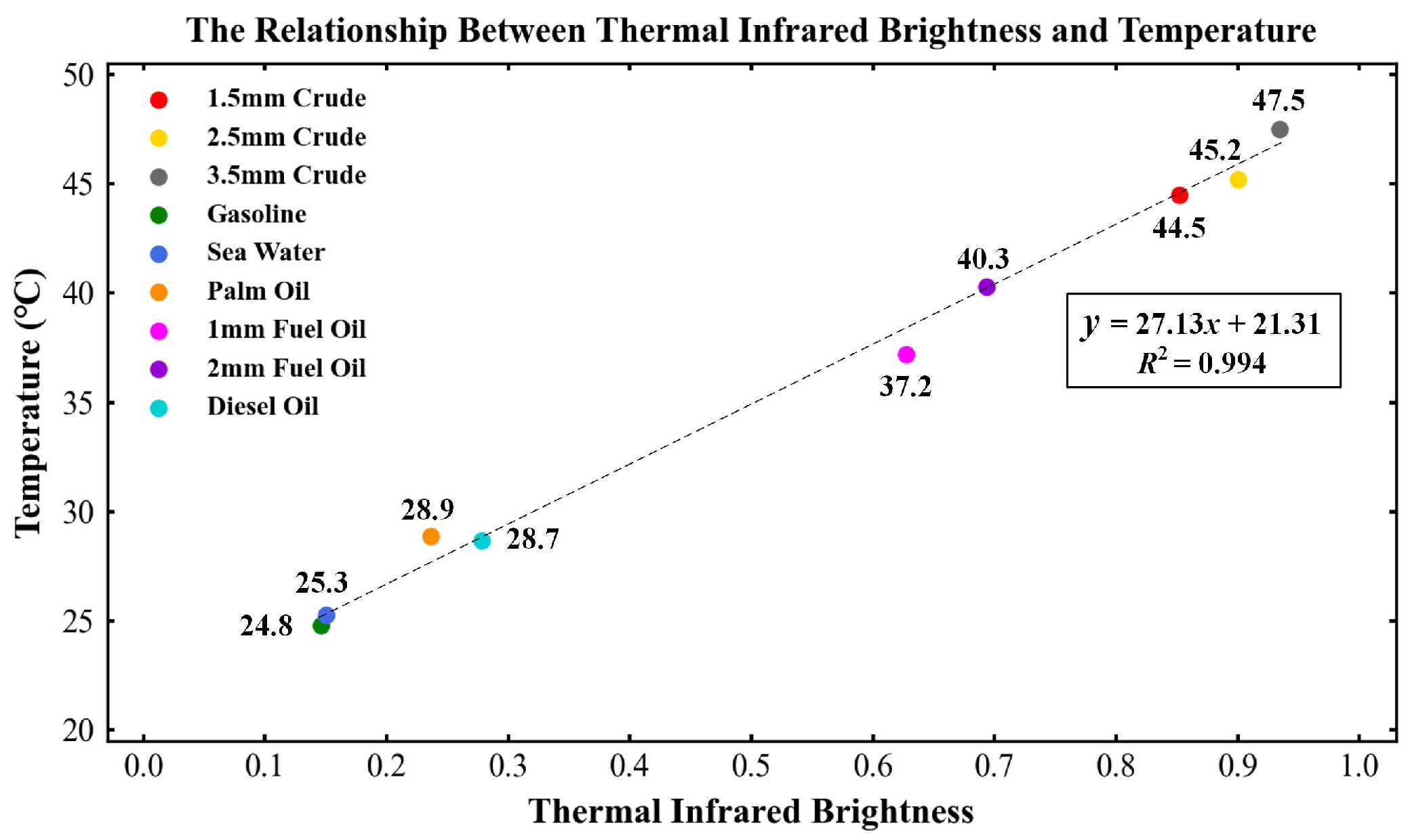
As shown in Figure 20, the surface temperature of each experimental group at T1 is positively correlated with the thermal radiation brightness with an R² of 0.994. We fit the kinetic temperature calibration polynomial model and performed batch thermal infrared temperature calibration on random samples of the oil spills. The thermal infrared temperature data of oil spills at T1 after calibration is shown in

Table 13. Thermal infrared temperature data of oil spill at T1.

	Temperature Information (°C)
Group	Average	Max	Min	STD
1#-1.5 mm Crude	44.4	46.0	42.3	0.97
2#-2.5 mm Crude	45.7	47.2	44.6	0.61
3#-3.5 mm Crude	46.6	48.1	43.1	1.06
4#-Gasoline	25.3	25.5	24.8	0.13
5#-Seawater	25.4	25.7	25.2	0.06
6#-Palm Oil	27.7	30.1	26.7	0.83
7#-1 mm Fuel Oil	38.3	40.9	37.4	0.79
8#-2 mm Fuel Oil	40.1	41.2	36.1	1.19
9#-Diesel Oil	28.8	29.1	27.3	0.48

.

As the results in Table 13 show, the oil film thermal infrared temperature of the heavy-oil experimental group is positively correlated with the thickness. A thicker oil film is associated with a higher temperature. In addition, the standard temperature deviations (STDs) of the heavy-oil groups are larger than that of the seawater and light-oil groups. We believe that the temperature STD can be used to characterize the uniformity of the oil film distribution on the sea surface. The light-oil films tend to diffuse evenly, so the temperature of each position of the oil film is relatively uniform with a small STD. Heavy oils have high surface viscosity, large surface roughness, and poor uniformity, leading to a relatively high-temperature STD.

Because of the low dimensionality of the thermal infrared remote sensing image data, deep learning is not suitable in this case. Instead, an SVM model was used to detect the oil spill, and the detection accuracy is shown in

Table 14. Accuracy of thermal infrared oil spill detection based on SVM.

	Index
Group	Recall (%)	Precision (%)	F1-Score
1#-1.5 mm Crude	74.24	68.37	0.712
2#-2.5 mm Crude	67.68	59.56	0.634
3#-3.5 mm Crude	68.18	87.66	0.767
4#-Gasoline	38.38	97.44	0.551
5#-Seawater	98.99	61.64	0.760
6#-Palm Oil	84.85	80.38	0.826
7#-1 mm Fuel Oil	85.35	76.82	0.809
8#-2 mm Fuel Oil	74.24	83.52	0.786
9#-Diesel Oil	79.29	83.96	0.816
OA (%)	74.58
Kappa	0.714
Time (min)	1.19

. The OA reaches 74.58%, Kappa reaches 0.714, and the detection time is 1.19 min. The detection accuracy F₁-score for heavy-oil films is larger than 0.634, and the recognition accuracy F₁-score for light-oil types is larger than 0.551. These experimental results demonstrate that there is potential for marine oil-spill detection research based on thermal infrared remote sensing images.

The temperature difference (TD) between the oil films determines the ability of thermal infrared remote sensing to detect oil spills. As shown in Table 12, from T1 to T3, as time passes, the oil film surface temperature of each experimental group tends to decrease. The gradual decrease in the solar elevation angle over time led to the decrease in sunlight intensity and the reduction in the heat absorbed by the oil film surface so that the surface temperature of the oil spill decreased over time. Heavy oil has a strong absorbing effect on sunlight, which increases the surface temperature of the oil film. Therefore, the surface temperature of the oil film of the heavy-oil group is higher than that of the light-oil and seawater groups at T1–T3. Moreover, for the heavy-oil groups, the surface temperature increased with increases in the thickness of the oil film. The surface temperatures of the crude oil and fuel oil groups differ substantially: the overall surface temperature of the crude oil groups is higher than that of the fuel oil groups.

At T3, the TDs between the light-oil and seawater groups was less than ±1.6 °C, the TD between the crude oil groups was less than ±0.2 °C, and the TD of the fuel oil group was less than ±0.5 °C. From this, we can infer that under strong light intensity, there is an obvious TD between light oils and seawater as well as between heavy-oil films with different thicknesses. The detection results further show that thermal infrared remote sensing technology has a certain potential for oil-spill detection. However, under low light intensity conditions, the TDs are small for light oils and seawater as well as for different heavy-oil films. This will affect the sensitivity of thermal infrared detection, thereby affecting the accuracy of oil-spill detection. In the future, hyperspectral and thermal infrared remote sensing technology will be combined to achieve coaxial multi-dimensional data acquisition of marine oil spills, which is expected to increase the feature extraction space of the deep learning model and improve the accuracy of oil-spill detection based on the ALTME optimizer proposed in this paper.

4. Conclusions

4.1. Conclusions

Marine oil-spill accidents seriously threaten both the marine ecological environment and human health. The type of oil spills and the thickness of the oil films are important basic items of information needed for scientific decision-making at the oil-spill site. In this study, an experimental setup was constructed to simulate real marine oil-spill scenarios to the greatest extent, and accuracy verification for the detection model was carried out. UAV imaging hyperspectral remote sensing technology was then used to investigate rapid and effective oil-spill detection. The ALTME optimizer, which is suitable for the characteristics of hyperspectral imagery and can adapt to different time phases of oil-spill scenarios, was proposed. Experimental results show that the ALTME optimizer can assign adaptive cumulative learning weights to multiple batches of long-term oil-spill spectral information to fully learn and utilize the spectral information. It effectively overcomes the problem of poor spectral separability among light oils, deeply learns the spectral differences between thick oil films, and then accurately identifies the type of oil spills and detects the thickness of thick oil films.

In this study, the ALTME optimizer was also evaluated on the Pavia University hyperspectral data, which are similar to the experimental data in terms of specifications. The results show that the optimizer exhibits excellent generalization and applicability, which make it suitable for hyperspectral detection research. This study also actively explored oil-spill detection based on thermal infrared remote sensing. Under strong sunlight, thermal infrared remote sensing technology has oil-spill detection potential.

4.2. Perspectives and Future Works

In this study, the sunlight intensity was obtained by calculating the solar elevation angle and then used to analyze its influence on the oil-spill spectrum curves. In the future, we plan to use a photometer to directly measure the sunlight intensity at different times. This study is an exploratory study of the oil-spill detection ability of the UAV hyperspectral sensor under ideal conditions. We plan to carry out oil-spill detection research under different sunlight conditions, strong winds, and other rough conditions in the future so as to explore the detection ability of the model proposed in this paper. In this study, we found that thick oil films with different thicknesses can be qualitatively detected by UAV hyperspectral sensors. In future research, we will carry out research on the quantitative inversion of oil film thickness on this basis.

Moreover, we found that thermal infrared remote sensing technology showed a certain potential for oil-spill detection under strong sunlight conditions. Our team intends to develop a coaxial multi-dimensional integrated sensor for both hyperspectral and thermal infrared data to obtain multi-dimensional remote sensing data of oil spills on the sea surface, thereby increasing the feature space of the deep learning model and improving the detection accuracy of marine oil spills.

References

- Yang, J.F.; Wan, J.-H.; Ma, Y.; Zhang, J.; Hu, Y.-B.; Jiang, Z.-C. Oil Spill Hyperspectral Remote Sensing Detection Based on DCNN with Multi-Scale Features. J. Coast. Res. 2019, 90, 332–339. [Google Scholar] [CrossRef]
- Jiang, Z.C.; Ma, Y. Research on crude oil film absolute thickness inversion based on self-expanding deep confidence network. Ocean. Sci. 2021, 45, 94–107. [Google Scholar]
- Sun, S.J.; Hu, C.M. The Challenges of Interpreting Oil-Water Spatial and Spectral Contrasts for the Estimation of Oil Thick-ness: Examples from Satellite and Airborne Measurements of the Deepwater Horizon Oil Spill. IEEE Trans. Geosci. Remote Sens. 2019, 5, 1–16. [Google Scholar]
- Velotto, D.; Migliaccio, M.; Nunziata, F.; Lehner, S. Dual-Polarized TerraSAR-X Data for Oil-Spill Observation. IEEE Trans. Geosci. Remote Sens. 2011, 49, 4751–4762. [Google Scholar] [CrossRef]
- Marghany, M. Utilization of a genetic algorithm for the automatic detection of oil spill from RADARSAT-2 SAR satellite data. Mar. Pollut. Bull. 2014, 89, 20–29. [Google Scholar] [CrossRef] [PubMed]
- Alpers, W.; Holt, B.; Zeng, K. Oil spill detection by imaging radars: Challenges and pitfalls. Remote Sens. Environ. 2017, 201, 133–147. [Google Scholar] [CrossRef]
- Ren, G.B.; Guo, J.; Ma, Y.; Luo, X.D. Hyperspectral remote sensing detection and thickness estimation method for sea surface oil spilled drones. Acta Oceanol. Sin. 2019, 41, 150–162. [Google Scholar]
- Shi, Q.; Liu, M.; Li, S.; Liu, X.; Wang, F.; Zhang, L. A Deeply Supervised Attention Metric-Based Network and an Open Aerial Image Dataset for Remote Sensing Change Detection. IEEE Trans. Geosci. Remote. Sens. 2021, 61, 1–16. [Google Scholar] [CrossRef]
- Lammoglia, T.; Roberto, C. Spectroscopic characterization of oils yielded from Brazilian offshore basins Potential applications of remote sensing. Remote Sens. Environ. 2011, 115, 2525–2535. [Google Scholar] [CrossRef]
- Yang, Q.Q. Application of Hyperspectral Oil Spill Image Feature Extraction in Oil Species Identification. Master’s Thesis, Dalian Maritime University, Dalian, China, 2010. [Google Scholar]
- Han, Z.; Wan, J.; Deng, L.; Liu, K. Oil Adulteration Identification by Hyperspectral Imaging Using QHM and ICA. PLoS ONE 2016, 11, e0146547. [Google Scholar] [CrossRef] [Green Version]
- Wu, X.; Song, J.M.; Li, X.G.; Yuan, H.M.; Li, N. Technical methods for obtaining oil spill volume at sea. Ocean. Technol. 2011, 30, 50–54. [Google Scholar]
- Song, S.S.; An, W.; Li, J.W.; Zhao, Y.P.; Jin, W.W. A review of research on marine oil spill assessment methods. Coast. Eng. 2017, 36, 83–88. [Google Scholar]
- Lu, Y.C.; Hu, C.M.; Zhan, W.F. Detecting and quantifying oil slick thickness by thermal remote sensing: A ground-based experiment. Remote Sens. Environ. 2016, 181, 207–217. [Google Scholar] [CrossRef]
- Lu, Y.; Shi, J.; Wen, Y.; Hu, C.; Zhou, Y.; Sun, S.; Zhang, M.; Mao, Z.; Liu, Y. Optical interpretation of oil emulsions in the ocean—Part I: Laboratory measurements and proof-of-concept with AVIRIS observations. Remote Sens. Environ. 2019, 230, 111183. [Google Scholar] [CrossRef]
- Lu, Y.C.; Shi, J.; Hu, C.M.; Zhang, M.W.; Sun, S.J.; Liu, Y.X. Optical interpretation of oil emulsions in the ocean-Part II: Ap-plications to multi-band coarse-resolution imagery. Remote Sens. Environ. 2020, 242, 111778. [Google Scholar] [CrossRef]
- Texeira, C.; Santos, S.; Aquino, N. Source identification of sea surface oil with geochemical data in Cantarell, Mexico. Micro-Chem. J. 2014, 117, 202–213. [Google Scholar] [CrossRef]
- Bayona, J.M.; Domínguez, C.; Albaigés, J. Analytical developments for oil spill fingerprinting. Trends Environ. Anal. Chem. 2015, 5, 26–34. [Google Scholar] [CrossRef]
- Yang, J.; Wan, J.; Ma, Y.; Zhang, J.; Hu, Y. Characterization analysis and identification of common marine oil spill types using hyperspectral remote sensing. Int. J. Remote Sens. 2020, 41, 7163–7185. [Google Scholar] [CrossRef]
- Liu, B.X.; Li, Y.; Han, L. Research on the Identification of Surface Oil Species Based on Spectral Reflectance Data. Spectrosc. Spectr. Anal. 2016, 36, 1100–1103. [Google Scholar]
- Shen, Y.F.; Liu, J.Q.; Ding, J.; Jiao, J.N.; Sun, S.J.; Lu, Y.C. HY-1C COCTS and CZI observation of marine oil spills in the South China Sea. J. Remote Sens. 2020, 24, 933–944. [Google Scholar]
- Wan, H.J.; Han, Z.Z.; Song, X.X.; Liu, J. Oil species identification method of marine oil spill hyperspectral imaging based on multi-mode fusion. Acta Lumin. 2016, 97, 473–480. [Google Scholar]
- Shi, J.; Jiao, J.; Lu, Y.; Zhang, M.; Mao, Z.; Liu, Y. Determining spectral groups to distinguish oil emulsions from Sargassum over the Gulf of Mexico using an airborne imaging spectrometer. ISPRS J. Photogramm. Remote Sens. 2018, 146, 251–259. [Google Scholar] [CrossRef]
- Fang, S.A.; Huang, X.X.; Yin, D.; Xu, C.; Feng, X. Research on UV reflectance characteristics of marine oil spill simulation targets. Spectrosc. Spectr. Anal. 2010, 30, 738–742. [Google Scholar]
- Hu, J.C.; Wang, D.F. Monitoring method of ocean oil spilling based on remote sensing. Environ. Prot. Sci. 2014, 40, 68–73. [Google Scholar]
- Shi, J. Study on Hyperspectral Remote Sensing of Marine Oil Emulsion. Master’s Thesis, Nanjing University, Nanjing, China, 2019. [Google Scholar]
- Lu, Y.C.; Tian, Q.J.; Wang, J.J.; Wang, X.C.; Qi, X.P. Experimental study on the spectral response of sea surface oil film. Chin. Sci. Bull. 2008, 9, 111–114. [Google Scholar]
- Lu, Y.C.; Tian, Q.J.; Li, X. Oil film thickness remote sensing inversion theory based on oil slick double-beam interference model. Sci. China Earth Sci. 2011, 41, 541–548. [Google Scholar]
- Lu, S. Research and Application of Hyperspectral Region Growth Algorithm Combined with Unmixing. Ph.D. Dissertation, Dalian Maritime University, Dalian, China, 2015. [Google Scholar]
- Jiang, Z.; Ma, Y.; Yang, J. Inversion of the Thickness of Crude Oil Film Based on an OG-CNN Model. J. Mar. Sci. Eng. 2020, 8, 653. [Google Scholar] [CrossRef]
- Chen, Y.; Jiang, H.; Li, C.; Jia, X.; Ghamisi, P. Deep Feature Extraction and Classification of Hyperspectral Images Based on Convolutional Neural Networks. IEEE Trans. Geosci. Remote Sens. 2016, 54, 6232–6251. [Google Scholar] [CrossRef] [Green Version]
- Hu, F.; Xia, G.-S.; Hu, J.; Zhang, L. Transferring Deep Convolutional Neural Networks for the Scene Classification of High-Resolution Remote Sensing Imagery. Remote Sens. 2015, 7, 14680–14707. [Google Scholar] [CrossRef] [Green Version]
- Yang, X.F.; Ye, Y.M.; Li, X.T.; Raymond, Y.; Zhang, X.F.; Huang, X.H. Hyperspectral Image Classification with Deep Learning Models. IEEE Trans. Geosci. Remote Sens. 2018, 56, 5408–5423. [Google Scholar] [CrossRef]
- Jiang, Z.; Ma, Y. Accurate extraction of offshore raft aquaculture areas based on a 3D-CNN model. Int. J. Remote Sens. 2020, 41, 5457–5481. [Google Scholar] [CrossRef]
- Zhang, H.; Li, Y.; Jiang, Y.; Wang, P.; Shen, Q.; Shen, C. Hyperspectral Classification Based on Lightweight 3-D-CNN With Transfer Learning. IEEE Trans. Geosci. Remote Sens. 2019, 57, 5813–5828. [Google Scholar] [CrossRef] [Green Version]
- Hu, A.N.; Xie, Z.; Xu, Y.Y.; Xie, M.Y.; Wu, L.; Qiu, Q.J. Unsupervised Haze Removal for High-Resolution Optical Remote-Sensing Images Based on Improved Generative Adversarial Networks. Remote Sens. 2020, 12, 4162. [Google Scholar] [CrossRef]
- Zorzi, S.; Maset, E.; Fusiello, A.; Crosilla, F. Full-Waveform Airborne LiDAR Data Classification Using Convolutional Neural Networks. IEEE Trans. Geosci. Remote Sens. 2019, 57, 8255–8261. [Google Scholar] [CrossRef]
- Yang, J.F. Marine Oil Spill Detection and Oil Types Identification Using Multi-Dimensional Optical Remote Sensing. Ph.D. Thesis, China University of Petroleum, Qingdao, China, 2021. [Google Scholar]
- Ling, J.M.; Li, L.; Wang, H.Y. Improved Fusion of Spatial Information into Hyperspectral Classification through the Aggregation of Constrained Segment Trees: Segment Forest. Remote Sens. 2021, 13, 4816. [Google Scholar] [CrossRef]
- Zhang, T.; Shi, C.; Liao, D.; Wang, L. Deep Spectral Spatial Inverted Residual Network for Hyperspectral Image Classification. Remote Sens. 2021, 13, 4472. [Google Scholar] [CrossRef]
- Fingas, M. The Challenges of Remotely Measuring Oil Slick Thickness. Remote Sens. 2018, 10, 319. [Google Scholar] [CrossRef] [Green Version]
- Hu, C.M.; Lu, Y.C.; Sun, S.J.; Liu, Y.X. Optical Remote Sensing of Oil Spills in the Ocean: What Is Really Possible? J. Remote Sens. 2021, 2021, 9141902. [Google Scholar] [CrossRef]
- Li, W.J.; Zhang, Z.Y.; Wang, X.J.; Luo, P. AdaX: Adaptive Gradient Descent with Exponential Long Term Memory. Comput. Sci. 2020, 5, 9740. [Google Scholar]
- Shazeer, N.; Stern, M. Adafactor: Adaptive Learning Rates with Sublinear Memory Cost. Comput. Sci. 2018, 4, 4235. [Google Scholar]
- Shi, Q.; Tang, X.; Yang, T.; Liu, R.; Zhang, L. Hyperspectral Image Denoising Using a 3-D Attention Denoising Network. IEEE Trans. Geosci. Remote Sens. 2021, 59, 10348–10363. [Google Scholar] [CrossRef]
- Liu, B.X. Extraction and Analysis of Oil Film on Water Based on Hyperspectral Characteristics. Ph.D. Thesis, Dalian Maritime University, Dalian, China, 2013. [Google Scholar]
- Sun, P.; Song, M.-P.; An, J.-B. Study of prediction models for oil thickness based on spectral curve. Spectrosc. Spectr. Anal. 2013, 33, 1881–1885. [Google Scholar]
Figure 1.
(a) Location of the experimental site and (b) aerial view of the experimental pool.
Figure 2.
DJI-M600PRO UAV and Cubert-S185 hyperspectral sensor.
Figure 3.
Installation of the PVC device.
Figure 4.
Oil spill experiment group labels.
Figure 5.
(a) Front view of the experimental oils and (b) top view of the experimental oils.
Figure 6.
Measuring the quality of the experimental oils. (a,b) are the process of crude oil measurement. (c,d) are the process of fuel oil measurement.
Figure 7.
(a–c) are on-site photos of the experiment.
Figure 8.
Oil spill hyperspectral images (red: 482 nm, green: 550 nm, blue: 662 nm) and sample label data of T1-T3. (a,d) are image and label data at T1, respectively. (b,e) are image and label data at T2, respectively. (c,f) are image and label data at T3, respectively.
Figure 9.
Structure of the marine oil spill detection 1D-CNN model.
Figure 10.
Remote sensing reflectance of the oil spills at T1.
Figure 11.
Remote sensing reflectance of the oil spills at T2.
Figure 12.
Remote sensing reflectance of the oil spills at T3.
Figure 13.
Detection results of the marine oil spill detection model. (a,e,i) are true color images at T1–T3, respectively (red: 482 nm, green: 550 nm, blue: 662 nm). (b,f,j) are detection results of the SVM model at T1–T3, respectively. (c,g,k) are detection results of the GRU model at T1–T3, respectively. (d,h,l) are detection results of the 1D-CNN model at T1–T3, respectively.
Figure 14.
Comparison of the detection accuracy of the marine oil spill detection model with the ALTME and Adam optimizers. (a) OA and Kappa coefficient of the detection results and (b) single accuracy F1-score of the detection results.
Figure 15.
Detection results of the oil spill detection model with the ALTME optimizer. (a,d,g) represent the true color images at T1–T3, respectively (red: 482 nm, green: 550 nm, blue: 662 nm). (b,e,h) are detection results of the basic 1D-CNN model at T1–T3, respectively. (c,f,i) are detection results of the 1D-CNN model with ALTME optimizer at T1–T3, respectively. The white boxes indicate incorrect recognitions obtained by the basic 1D-CNN model.
Figure 16.
Comparison of the loss values of the ALTME and Adam optimizer. (a,c,e) are loss values of the Adam optimizer at T1–T3, respectively. (b,d,f) are loss values of the ALTME optimizer at T1–T3, respectively.
Figure 17.
Time of ALTME optimizer cumulative learning weight adaptive selection.
Figure 18.
Recognition results for the public hyperspectral remote sensing data of Pavia University. (a) True color image (red: 50 band, green: 23 band, and blue: 5 band). (b) Sample labels. (c) Results of SVM. (d) Results of the 1D-CNN. (e) Results of 1D-CNN with the ALTME optimizer.
Figure 19.
(a,b) are thermal infrared remote sensing image and data labels.
Figure 20.
Relationship between thermal infrared brightness and oil spill temperature.