
Satellite Time Series and Google Earth Engine Democratize the Process of Forest-Recovery Monitoring over Large Areas


1
Alberta Biodiversity Monitoring Institute, Edmonton, AB T6G 2E9, Canada
2
Department of Geography, University of Calgary, Calgary, AB T2N 1N4, Canada
*
Author to whom correspondence should be addressed.
Remote Sens. 2021, 13(23), 4745; https://doi.org/10.3390/rs13234745
Submission received: 5 October 2021
/
Revised: 12 November 2021
/
Accepted: 19 November 2021
/
Published: 23 November 2021
(This article belongs to the Special Issue Feature Paper Special Issue on Forest Remote Sensing)
Abstract
:Contemporary forest-health initiatives require technologies and workflows that can monitor forest degradation and recovery simply and efficiently over large areas. Spectral recovery analysis—the examination of spectral trajectories in satellite time series—can help democratize this process, particularly when performed with cloud computing and open-access satellite archives. We used the Landsat archive and Google Earth Engine (GEE) to track spectral recovery across more than 57,000 forest harvest areas in the Canadian province of Alberta. We analyzed changes in the normalized burn ratio (NBR) to document a variety of recovery metrics, including year of harvest, percent recovery after five years, number of years required to achieve 80% of pre-disturbance NBR, and % recovery the end of our monitoring window (2018). We found harvest areas in Alberta to recover an average of 59.9% of their pre-harvest NBR after five years. The mean number of years required to achieve 80% recovery in the province was 8.7 years. We observed significant variability in pre- and post-harvest spectral recovery both regionally and locally, demonstrating the importance of climate, elevation, and complex local factors on rates of spectral recovery. These findings are comparable to those reported in other studies and demonstrate the potential for our workflow to support broad-scale management and research objectives in a manner that is complimentary to existing information sources. Measures of spectral recovery for all 57,979 harvest areas in our analysis are freely available and browseable via a custom GEE visualization tool, further demonstrating the accessibility of this information to stakeholders and interested members of the public.
1. Introduction
Forests are a vital element of the Earth’s environment, supporting biodiversity [1], maintaining soil health and clean air [2,3,4], providing cultural and ecosystem services [5,6], and mitigating climate change [7,8]. These facts are now well-established in the scientific literature and, increasingly, in the broader public consciousness. This latter trend is evidenced by international initiatives such as the 2011 Bonn Challenge [9] and the 2014 New York Declaration on Forests [10], which aim to restore hundreds of millions of hectares (mha) of forest worldwide. More recently, the Strategic Plan for Forests 2017–2030 adopted by the United Nations (UN) General Assembly in April of 2017 [11] provides a framework for global action on sustainable forest management and the halting of forest degradation and deforestation.
Achieving these global forest initiatives successfully will require effective mapping, monitoring, and assessment of forest cover and health. As a result, we require accurate, comprehensive, up-to-date knowledge of baseline or current conditions, alongside subsequent change. Forest ecosystems across the globe undergo continual change by both natural and anthropogenic forcing; thus, a critical component for supporting programs such as the UN’s Strategic Plan is the mapping of forest disturbance and recovery.
Large-area mapping and monitoring of forests is most effectively undertaken through remote sensing. Earth observation (EO) satellites offer global-level synoptic, repeating views of the planet. Their use for gathering information on forested landscapes began with the launch of the first civilian EO satellite, Landsat, in 1972 [12]. Within twenty years, satellite remote sensing of the world’s forests was an established practice [13], and has only continued to expand in scope and maturity alongside technological advances in satellite sensors, computer hardware and software (e.g., cloud computing), and analytical techniques such as machine learning [14].
The potential of EO remote sensing for mapping forest disturbance and recovery has likewise grown significantly, as evidenced by the literature. For instance, ref. [15] synthesized published results on remotely sensed forest disturbance and recovery within the context of impacts on biomass and canopy cover, and estimated that roughly 400,000 to 700,000 km2 of forest were disturbed each year across the globe by large-scale, abrupt events (e.g., fire, logging, conversion to agriculture). The more recent global, Landsat-based analysis of forest extent, loss, and gain from 2000 to 2012 revealed a net loss of 1.5 million km2 of forest cover over this period [16].
1.1. Remote Sensing of Forest Recovery
Forest gain is not as easily or as frequently measured and detected with remote sensing as forest loss [17], because it is a slower, ongoing, and often more complex process than the sudden, abrupt events that comprise many disturbances [18,19]. Nevertheless, identifying forest gain is as essential to forest cover mapping as identifying forest disturbance, and is often an outcome of post-disturbance recovery. This is especially true of Canada’s northern boreal forests, where multifaceted disturbance regimes that include fires of varying intensities, insect outbreaks, petroleum resource extraction, and forestry lead to a complex patchwork of diverse and dynamic forest ecosystems at varying stages of recovery [20].
Mapping and monitoring forest recovery across Canada’s boreal forests, which are largely remote and cover 270 mha, is a challenging undertaking. Ref. [21] synthesized findings from roughly a dozen local-level, ground-based forest recovery studies that focused on post-fire or post-harvest canopy cover, tree height and/or stand stem diameter. Their study reported average recovery rates to 10% canopy cover and average heights of 5 m to be five to 10 years after fire or harvest. However, the authors noted significant variability across ecozones, forest species composition, and between these two disturbance types. While ref. [21] provided an informative analysis, the authors also acknowledged the limits of their work, which was constrained to fine spatial scales, a limited number of studies, and limited stand age ranges [21]. These issues illustrated the difficulties of ground-based data collection in remote boreal forests, and the authors advocated for EO-based remote sensing as a means of overcoming these challenges.
The advantages of EO approaches for forest mapping in Canada are well-recognized, and leveraged by researchers, government, and industry alike. The Earth Observation for Sustainable Development of Forests, a partnership project between the Canadian Forest Service and the Canadian Space Agency, produced a EO-based landcover map of Canada’s forested area circa 2000 [22]. The product’s aim was to support provincial- and national-scale sustainable forest management and biomass reporting, but has also been used elsewhere for numerous purposes such as wildfire susceptibility and habitat fragmentation assessments, to name a few [23,24]. Other large-scale applications of EO over Canadian forests include burn mapping [25,26,27], forest condition monitoring [28,29], and biodiversity assessment [30,31]. However, it is important to note here that remotely sensed forest condition, disturbance, and recovery capture changes in land surface spectral signatures as a proxy for such things as fire severity, deforestation, or regrowth and regeneration, rather than direct estimates of particular vegetative or tree characteristics.
Large-scale EO remote sensing of post-disturbance forest recovery in Canada has necessarily relied upon analyses of Landsat image time series. Not only is the Landsat program the longest running, continuous, systematic source of global land surface satellite imagery, it also provides multiple images per year at a spatial resolution (30 m) suited to detecting many landscape changes of interest, including fire- and forestry-related dynamics [32,33]. For instance, ref. [17] examined Landsat-derived Tasseled Cap Greenness and Wetness [34] time series in stand-replacing forest disturbances across the eastern and western portions of the Canadian Boreal Shield, comparing spectral recovery trajectories post-wildfire and post-harvest to those of undisturbed areas. The authors noted not only different patterns of disturbance between these two regions, but also greater differences in recovery trajectories, suggesting that differences in disturbance regimes, climate regimes, stand initiation processes, and soil conditions may all play a role. Ref. [35] used a different approach, reconstructing successional trajectories using multi-temporal Landsat image classifications in particular harvest and wildfire disturbances in Quebec, Canada, to compare changes in vegetation composition through time. They found that harvested forest generally started from a more advanced development stage and thus showed faster rates of succession. However, the greater heterogeneity of environments in which wildfires are located, which includes unproductive sites, led to overall slower rates of succession in these features [35]. The latter differences lessened when only productive forest and wildfire sites were compared.
Both [17,35] provided important insights into remotely sensed post-disturbance forest recovery trajectories, and discussed how these vary across time and space alongside a number of important factors. However, both studies were limited in their geographical extent to a sample of Landsat scenes or a particular region. Ref. [19] provided a broader view of forest dynamics at a national level. In a Canada-wide remote sensing analysis of stand-replacing forest disturbance and recovery, the authors used the normalized burn ratio or NBR derived from Landsat time series [36] to identify 57.5 mha of disturbed forest. Analyzing spectral recovery at these sites, they found that harvested areas are generally recovering more rapidly than burned areas when disturbance magnitude is considered. Ref. [19] again noted variability in this recovery across Canada’s ecozones, finding lower rates of longer-term forest spectral recovery in the Taiga Shield East and Montane Cordillera, than in others such as the Boreal Shield East.
1.2. Motivation and Objectives
National-scale forest spectral recovery information such as that compiled by [19] is critical for accurate forest cover mapping across Canada. As recovery is an ongoing process, however, frequent updating is needed for continued monitoring, and these authors’ approach relies on specialized, high-performance computing. As a result, its implementation can be limited by access to such resources. New tools and technologies in the form of publicly accessible, cloud-based geospatial data storage and processing services (e.g., Google’s Earth Engine, Microsoft’s Planetary Computer, and Amazon’s Earth on AWS) have begun to democratize the use of large-volume EO datasets for landscape analyses at unprecedented spatial and temporal scales [37,38,39]. Such services offer a new opportunity for widely accessible, effective, repeatable, and adaptable approaches to mapping spectral recovery over extensive forested landscapes.
In this work, we bring together publicly accessible, cloud-based services, the lengthy Landsat archive, open-access disturbance event layers, and published spectral recovery methods in a novel manner to produce large-scale, remote sensing-based information on post-disturbance forest recovery within a Canadian context. At present, no published studies have leveraged such cloud-based services to implement Landsat time series-based spectral recovery in Canadian boreal forest landscapes at large scales. In addition, our use of existing information on forest disturbance location and extent for directing our analyses is unique—disturbance events are typically remotely sensed before recovery is extracted (e.g., [17,18,40]).
Our objectives are as follows: (i) to develop easily reproducible, adaptable, and scalable methods for generating updated maps of spectral recovery in forest disturbances; (ii) to generate a publicly available forest spectral recovery dataset for the Canadian province of Alberta; (iii) to support the science-to-knowledge translation of our results through a data visualization tool; and (iv) to compare patterns of forest spectral recovery across different ecological regions within our province.
We specify the term spectral recovery here to distinguish it from more specific, ground-observed forest compositional, structural, functional, or ecosystem recovery. Spectral recovery reflects the recovery of land surface spectral signals, which respond to the growth and development of green vegetation but are not necessarily a direct indicator of specific surface vegetation characteristics. Spectral recovery is nevertheless a useful indicator for characterizing forested areas as they revegetate after disturbance, and has been shown to relate to vegetation structure and cover metrics derived from LiDAR and ground measurements [41,42].
We use the province of Alberta, Canada and its harvested forest areas as a test case for this work. Not only does a large portion of the Alberta landscape comprise managed, harvestable forest, but the province is also uniquely rich in geospatial data. These include provincial LiDAR and multi-annual SPOT image mosaics, large volumes of environmental sensor data from audio and photographic devices, and most especially, up-to-date human footprint data layers (e.g., [43,44]).
While both wildfire and harvest are primary sources of forest disturbance within Alberta [45] and are both easily detectable and monitored using satellite remote sensing, we focus here on recovery in forest harvest areas. This is for two reasons. First, they are anthropogenic in nature and thus managed—i.e., subject to government legislation and mandatory reforestation standards. As a result, their on-the-ground recovery is monitored at the local level, and these local-level understandings would benefit from broader, regional- to provincial-level characterizations of recovery status and trends. Second, the remote sensing of post-harvest forest recovery is less well studied than that of post-fire recovery, and there is, therefore, a larger knowledge gap in spectrally assessing levels of recovery in the former features. Developing a repeatable workflow and test case dataset of post-harvest forest spectral recovery offers a starting point for future research and study over national scales or in other jurisdictions.
The following sections describe our workflow, largely undertaken using Google Earth Engine, our final forest harvest area spectral recovery output, and some tools for its dissemination and visualization. Finally, we present a short statistical analysis of post-harvest forest spectral recovery across Alberta’s different ecological regions and subregions.
2. Materials and Methods
2.1. Study Area
Our study area comprises the harvested forest areas of Alberta, in western Canada (Figure 1). Approximately 60% or nearly 40 mha of Alberta’s 66 mha are forested, and 38 mha or roughly 95% of this forested area is public land [46]. With the exception of parks and protected areas, much of this area is under active management through Forest Management Agreements [47].
Ranging across both elevational (200 m to >1200) and latitudinal gradients, Alberta’s harvestable forests cover a wide variety of climatic conditions, topographies, and ecosystems. These include deciduous-leading upland mixedwoods in the central, eastern, and northeastern boreal, which experience short, warm summers and long, cold winters [48]. Deciduous-dominated upland forests in the northwestern and south-central boreal reflect warmer summers and milder winters, while more diverse upland mixedwood forests are found in the northwestern boreal, where moister and cooler conditions prevail [48]. Mixedwood and coniferous-dominated harvestable forests dominate the foothills and montane regions of southwestern Alberta, where colder, snowier winters and shorter, wetter summers dominate the climate, and where large elevational gradients and aspect are a strong driver of forest composition [48]. Common coniferous tree species include white spruce (Picea glauca), black spruce (Picea mariana), jack pine (Pinus banksiana), lodgepole pine (Pinus contorta var. latifolia), and balsam fir (Abies balsamea), while common deciduous species include trembling aspen (Polpulus tremuloides), balsam poplar (Populus balsamifera), white birch (Betula papyrifera), and tamarack (Larix laricina) [46,48].
2.2. Characterizing Spectral Recovery
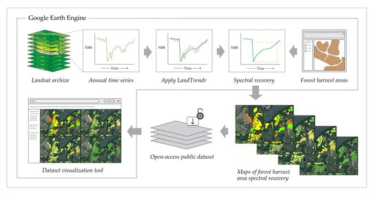
An overview of our workflow is shown in Figure 2. Much of this was implemented online in Google Earth Engine (GEE) using the JavaScript programming interface [49], but portions were conducted in a desktop environment using Esri’s ArcGIS 10.6.1 [50], and the R Statistical Package [51], implemented using RStudio [52].
Our workflow compiled imagery from Landsat 5, 7, and 8 into an annual composite image stack, extracted a series of spectral metrics related to post-harvest vegetative recovery, and derived per-harvest-area statistics. The following sections describe our datasets and pre-processing, spectral trajectory analysis, and quality-control measures. As one of our objectives is to produce a published, open-access dataset for Alberta harvest areas, this last step is an important one.
2.2.1. Datasets and Preprocessing
Unlike many other forest recovery remote sensing studies that first detected forest disturbance before describing recovery, we leveraged an existing dataset to inform the location and boundaries of the Alberta harvest areas that are the focus of this work. We used harvest-area polygons from the Alberta Biodiversity Monitoring Institute’s (ABMI’s) latest Human Footprint Inventory (HFI 2018) to define our units of analysis.
The HFI is a spatially explicit, digital database of visible human footprint features across the province in Alberta, and includes 20 categorical sublayers with over 110 specific feature types [53]. As the product of the careful compilation of multiple existing datasets, in combination with updating by trained interpreters using high-resolution satellite imagery, the HFI presents a uniquely consistent, comprehensive source of information on anthropogenic disturbance across Alberta’s forests. The product is updated annually, with yearly products from 2014 onward. The dataset contains 231,883 harvest-area polygons dating from the 1920s onward, and ranging in size from <1 hectare (ha) to >2000 ha. The HFI’s harvest-area sublayer is based upon digital forest inventories compiled by the forest industry itself, as part of Forest Management Agreements with the province of Alberta. Such agreements are the mechanism by which forestry land tenure and harvesting rights are granted in the province, and require the industry to provide accurate, up-to-date forest inventories as part of their management plan [54].
To preprocess harvest-area polygons, we first extracted the harvest-area sublayer from the full HFI geodatabase and buffered it using a negative 30 m distance. This was intended to remove the outer 30 m of each polygon and, thus, minimize the risk of edge effects resulting from variations or misalignments with 30-m Landsat imagery. The buffered polygons were then simplified by removing extraneous vertices while maintaining a 15 m boundary shift tolerance. This was undertaken to reduce overall file size, and visual inspection of the result showed good similarity in size and form between pre- and post-simplification polygons. Finally, harvest-area polygons of less than 900 m2 (the area of one Landsat pixel) were removed and excluded from further analysis. We then uploaded the result as a shapefile table asset into GEE.
All image processing and spectral recovery calculations were performed using custom scripts in the GEE online environment [49]. Imagery from Landsat 5 Thematic Mapper (L5-TM), the Landsat 7 Enhanced Thematic Mapper + (L7-ETM+), and the Landsat 8 Operational Land Imager (L8-OLI) surface reflectance products, provided by the U.S. Geological Survey and spanning 1984 through 2018, comprised our satellite datasets. These data were atmospherically corrected using the Landsat Ecosystem Disturbance Adaptive Processing System [55] and were accompanied by cloud, shadow, water, and snow masks calculated using the CFMask algorithm [56]. We used the latter to remove affected pixels in all images and calibrated the L8-OLI imagery to spectrally match the L5-TM and L7-ETM+ products, using published coefficients provided by [57]. We then combined the images from all three sensors into a single, chronologically ordered image stack. This stack was transformed into annual composites by extracting per-pixel, growing season spectral median values for each band and year, wherein only images from the months of June through September were used (Figure 2). The intent was to remove extreme values and remaining unwanted noise (e.g., remaining haze), and to minimize snow effects, to produce annual composites that approximated a “best” representative growing season value for each pixel.
Our workflow next generated a normalized burn ratio (NBR) image from each annual composite multi-band image using Equation (1) [36], which uses the near-infrared (NIR) and shortwave-infrared (SWIR) reflectance Landsat bands (i.e., Bands 4 and 7, respectively, for L5-TM and L7-ETM+; Bands 5 and 7, respectively, for L8-OLI). Following the observed interactions between these spectral bands and land surfaces, the NBR increases with more complex vegetative structures and greater land surface moisture content [58,59,60], such as that found in forested landscapes. The index consequently drops as the amount and complexity of vegetation decreases (i.e., shrub or grassland) or is removed, and vegetative and soil moisture levels likewise decrease. The NBR thus shows good performance in responding to forest disturbance and recovery [18], and is well used for these purposes in the literature [61,62,63]. As with other normalized difference indices, NBR values are unitless, ranging from −1 to +1 and calculated as:
where NIRreflectance and SWIRreflectance are spectral reflectance in the NIR and SWIR bands, respectively.
Annual Landsat NBR image composites for the study were processed using the LandTrendr algorithm described by [18], and made widely available by the authors within the GEE environment [64]. LandTrendr iteratively fits a set of linear regression lines or segments and vertices to per-pixel annual spectral index time series to capture important shifts and trends in the time series, while also minimizing unwanted noise. This approach has been used successfully to not only detect forest disturbance [17,65,66,67], but also to examine post-disturbance spectral recovery [68,69,70]. After testing over a number of Alberta forest harvest areas, we chose to use LandTrendr’s default parameters for this work, with the exception of the recovery threshold. Based on our testing, we reset the latter from 0.25 to 0.5, which we found allows for quicker recovery rates within a single segment of the time series. We found that this better captured post-harvest NBR spectral changes in our particular study area. Once generated, the LandTrendr-fitted NBR time series were used to extract spectral recovery information.
2.2.2. Identifying Relevant Pixels
Our use of an existing harvest-area polygon dataset in place of remote sensing-based disturbance detection for determining areas of harvest required us to be cautious in selecting pixels that were used for calculating spectral recovery and generating per-harvest-area summaries, for several reasons. First, while it is a detailed and comprehensive dataset, the ABMI HFI nevertheless contains errors in its delineations, and can include multiple distinct harvest events within the boundary of a single polygon. Secondly, retention—the practice of leaving intact patches within a harvest area—is a common practice in Alberta [54]. Third, it is not uncommon for other natural or anthropogenic disturbances such as fires or petroleum well pads to also occur in harvested areas, and to therefore influence spectral trajectories. Finally, the ABMI HFI comprises harvest areas that date back as early as the 1920s, meaning that a significant portion of them were harvested before our Landsat time series began in 1984, and many were spectrally recovered well before this date.
For the purposes of this work, we removed pixels that fell within or intersected our processed harvest-area polygons and showed signs of influence from one or more of the factors listed in Table 1. As one of our objectives is to characterize post-harvest spectral recovery specifically, we did not want to include these confounding effects in our analyses. Such effects are undoubtedly of interest for understanding full landscape post-harvest recovery trends, and should be studied further, but such analyses are not within our scope here.
We also removed pixels for which detected harvest events occurred too early in the time series for us to calculate pre-harvest spectral conditions, or where they occurred too late in the time series for our spectral recovery metrics to be derived (i.e., within the first five years or last five years of our Landsat NBR time series). See Section 2.2.1 below for a description of how these metrics are calculated.
2.2.3. Spectral Recovery Metrics
While the ABMI HFI harvest areas possessed a year of harvest attribute, this information had been compiled from a variety of sources, as were the polygons themselves [53], and could vary in its accuracy. Our workflow relied on within-pixel spectrally detected harvest events as part of our metric calculations, as well as for post-processing (see Section 2.2.4). Therefore, we did not use the HFI year of harvest in our analyses, and used spectrally detected harvest events instead.
We identified a harvest event as an inter-annual drop in NBR of 0.2 or greater in the temporally segmented trajectory. We assumed that this drop represented a spectrally detectable forest harvest event since we were only examining pixels within or intersecting our preprocessed harvest-area polygons, and used the flags described in Section 2.2.2 to remove inappropriate pixels from our analysis. We selected the 0.2 NBR threshold after careful inspection of numerous harvest areas. Since we also observed that signals can decrease for more than one consecutive segment before beginning to increase (which signals the start of recovery), we identified the start of recovery (Recovstart) as the year after which we observed that the NBR had ceased to decrease, and had begun to increase (Figure 3). Given that spectral signals in our study area can drop over the course of more than one year during a harvest event, and that when a significant drop between two years is observed we assume that a disturbance has already occurred by the time of that second year, we ascribed the year of the detected harvest event (Harvestyr) to the first year before the detected drop (Figure 3). The period between Harvestyr and Recovstart was defined as Recovlag.
We used Harvestyr and Recovstart to calculate three post-disturbance spectral recovery metrics from LandTrendr-fitted NBR time series, on a per-pixel basis. The first was five-year percent spectral recovery (Recov%5yr), which is a relative measure of short-term recovery that is very similar to the Recovery Indicator (RI) metric described by [61] and used elsewhere [19,40,41,42]. It represents the percent of pre-harvest NBR spectral signal that is regained after five years of recovery, and is calculated as:
where:
and where NBRpreDistb is the mean NBR value for the five years leading up to the detected harvest event, NBRmin is the NBR value occurring in the year of Recovstart (i.e., the lowest NBR value reached after the harvest), and NBR5yr is the NBR value reached five years after Recovstart (Figure 3). We chose to use a pre-harvest five year window for calculating NBRpreDistb, rather than a shorter time period as is the case elsewhere (e.g., [19,62]), so as to minimize the effects of inter-annual variation due to atmospheric or other noise sources. As our calculation of this metric was slightly different from the original Recovery Indicator [61], we here elected not to label it as such. Aside from using a longer pre-harvest period to characterize NBRpreDistb, our metric differed largely in that it used the five years following Recovstart—the point at which spectral signals began to increase—rather than simply using the five years directly following the detected harvest event, as is the case in calculations of the RI. The intent was to account for instances where spectral signals in NBR time series dropped over the course of more than one year, which we observed to occur for some harvest areas within our study area. We therefore included only those years where spectral recovery was occurring in our metric calculations. Nevertheless, our Recov%5yr was found to be comparable to the RI.
Recov%5yr = (NBR5yr − NBRmin)/(NBRtotDistb) × 100,
NBRtotDistb = NBRpreDistb − NBRmin,
Our second spectral recovery metric, which reflects longer-term rates of recovery, was years to 80% recovery (Y2R). Described by [62], and again, also used elsewhere (e.g., [19,41,42,71,72]), it represents the length of time a harvest area’s NBR spectral signal requires to reach and exceed 80% of its pre-harvest levels as defined by NBRpreDistb.
We selected our final spectral recovery metric as a means of providing stakeholders and users of the final dataset with information reflecting the current state of spectral recovery in Alberta harvest areas. Recov%endTS is the percent spectral recovery observed at the end of the time series (i.e., 2018), and is calculated as:
where NBRlast is the NBR value in the last year of the time series. Unlike our first two metrics, this measure of spectral recovery is not found in the published literature. As our time series spanned several decades, and the majority of harvest areas in our dataset were likely to have spectrally recovered by its end, this metric offered a recent glimpse into which harvest areas’ spectral signals were still recovering, and more particularly, which were showing delayed recovery.
Recov%endTS = (NBRlast − NBRmin)/(NBRtotDistb) × 100,
As the above metrics were calculated at the per-pixel level, we summarized these for each harvest-area polygon in our dataset by extracting the mean and standard deviation of each from the relevant pixels corresponding to each polygon (i.e., those that remained unflagged for any confounding conditions). We also summarized the percent of all pixels corresponding to each harvest area that were flagged for the various conditions, and calculated the percent of all pixels that were used in final harvest-area summaries. The resulting statistics were exported in text file format from GEE, and then were post-processed in the R/RStudio and ArcGIS environments before being rejoined with the ABMI HFI harvest area polygons as an additional set of attributes.
2.2.4. Post-Processing and Quality Control
Since one of our objectives is a final dataset suitable for public distribution, our workflow included a set of post-processing and quality-control steps. These were performed on per-harvest-area summary outputs from GEE using R scripts written within RStudio. After formatting the output text files into a traditional data table, we calculated a series of relative confidence scores for the harvest areas. The intent of these was to provide relative measures of reliability, since our harvest area spectral recovery data were quite variable with regard to sufficient pixel representation, size, and within-polygon variability. We placed higher confidence, as reflected in higher scores, on greater pixel representation, larger sizes (i.e., greater numbers of pixels used for calculation), and greater homogeneity within a harvest-area polygon. We used descriptive statistical analyses (e.g., histograms) and personal observations of the data to create our confidence scores. They are further described in Table S1, found in our supplementary documentation. We summed the individual confidence scores to produce per-harvest-area total confidence scores. These offered an ordinal-level, relative ranking of harvest area metric reliability, which we used for quality control of the final dataset.
On the basis of flag results and relative confidence scores, data for harvest areas meeting any of the following criteria were removed both from the final public dataset, and from further analyses: (i) >50% of the pixels within or intersecting the harvest area were flagged and removed; (ii) fewer than nine pixels remained within a harvest area for metric calculations; (iii) a Harvestyr confidence score below four suggested that the polygon did not represent a single, homogeneous harvest event (Table S1); or (iv) the total confidence score was three or more standard deviations below the dataset mean.
Following the above quality-control measures, the remaining harvest area spectral recovery metrics were rejoined to the original ABMI HFI harvest-area polygons, within the ArcGIS environment. The final steps of our workflow were designed to further minimize additional human footprint and wildfire effects. Data from those harvest areas that overlapped other ABMI HFI human footprint features (e.g., mines, cultivation), and wherein this overlap constituted more than 20% of their area, were removed. We undertook this step to reduce the risk that spectral signals had been affected by other anthropogenic activities post-harvest. Visual inspection showed that those harvest areas that were overlapped by other HFI features by less than 20% were often overlapped by roads or wellsites—features we assumed were not captured in our metric calculations due to the use of the previously described flagging system.
The effects of wildfire on post-harvest spectral recovery metrics were reduced by removing data for those harvest areas overlapped by wildfires in the Government of Alberta’s most recent Wildfire Perimeter database [73] that had occurred within the 20 years prior to the detected harvest date or any time after the harvest date, and which occupied more than 10% of the harvest-area polygon. The 20-year threshold was chosen because, in most cases, we observed the spectral signals to have returned completely to pre-disturbance levels by this time after a single disturbance event (i.e., the spectral signal had generally saturated after 20 years).
The result of the above comprised our final, publicly distributable harvest area spectral recovery dataset wherein those harvest areas for which spectral recovery was reliably extracted had these metrics provided as an additional set of new attributes.
2.3. Public Dissemination of the Dataset
Once compiled, we made our final dataset available online as an open-access GIS layer through the ABMI website (www.abmi.ca). We also summarized important information pertaining to our methodology and the data themselves in a technical document, which we provided alongside the dataset. By making the dataset publicly available, we enabled its widespread use by a variety of stakeholders for diverse purposes, which could include land and resource management, ecological or wildlife conservation efforts, or community knowledge and engagement, among others.
Finally, we used GEE to develop and host an online data visualization tool or application that allows users to browse maps of key spectral recovery metrics provided in the final dataset within an accessible and friendly environment. Such a tool is important in the science-to-knowledge translation of geospatial data for a broad set of users with varying backgrounds and skill sets. While providing a dataset via a publicly available platform is key to it use beyond a narrow range of applications, support in the form of an easily accessible data exploration tool greatly increases the data’s usability. Both these steps directly support the further democratization of EO-based information products for all audiences.
2.4. Regional Analysis
The final step in our analysis was to examine spectral recovery in Alberta forest harvest areas as it varies by Natural Region and Subregion, in the hopes that broad spatial patterns in recovery, reflecting variations in topography, climate, and vegetative community, may be revealed. Ref. [48] divided Alberta’s varied landscapes into six Natural Regions—Rocky Mountain, Foothills, Grassland, Parkland, Boreal Forest, and Canadian Shield—and 21 Natural Subregions. The province’s harvestable forests fell largely within the Boreal Forest, Foothills, and Rocky Mountain Regions. We summarized the spectral recovery for each of these and their corresponding Subregions, while restricting our analyses to those harvest areas that fell completely within a single Subregion. It is important to note that some harvest areas did not reach 80% spectral recovery by the end of the studied time period; these were not included in any analyses of the Y2R metric. We used a one-way ANOVA for independent samples, and post-hoc Tamhane’s T2 statistics to check for statistically significant differences. The latter is a conservative pairwise comparison that accounts for unequal variance between groups [74]. These tests were performed with IBM’s SPSS Statistics 27 [75].
3. Results
3.1. Harvest Area Spectral Recovery
Preprocessing of the 231,883 harvest-area polygons comprising the ABMI’s 2018 HFI dataset produced an output of 177,604 polygons, which we uploaded into the GEE environment. After calculating spectral recovery metrics, processing and joining the resulting GEE outputs to HFI harvest-area polygons, and then conducting additional post-processing, our final dataset provided spectral recovery information for 57,797 forest harvest areas. Table 2 presents general statistics summarizing our results, while Figure 4 shows key spectral recovery metrics mapped over Alberta.
The distribution of pre-harvest spectral signatures (NBRpreDistb) was fairly narrow, falling for the most part between 0.600 and 0.700, given a mean of 0.647 and standard deviation (s.d.) of 0.048 (Table 2). This distribution was not surprising since harvested forest areas are generally likely to be similar in age and structure—i.e., mature, merchantable stands. This rendered comparisons of results across harvest areas more meaningful than if this metric were more dispersed in its distribution, as it indicated spectral homogeneity in pre-harvest conditions across our studied harvest areas.
Year of spectrally detected harvest event (Harvestyr) filled the full range of possible harvest dates—1989 to 2013. These dates reflected the reserving of the first and last five years of the time series for metric calculations. The mean Harvestyr of 2001.51 fell directly in the middle of this 24-year range (Table 2). Our time period of interest was represented well within the final dataset. The mean number of years between the Harvestyr and start of recovery (Recovstart), referred to as Recovlag, was 1.26, with an s.d. of 0.43. This indicated that the majority of detected harvest events represented by our dataset were single-season timber clearing events.
Harvest areas in our final dataset regained an average of 59.9% of their pre-harvest spectral signals after five years of recovery (Recov%5yr), though with considerable range and variability around this mean (s.d. = 18.3%; range = 1.86% to 168.5%; Table 2). We observed a similarly high level of variability and range for the years to 80% spectral recovery metric (Y2R), with a mean of 8.70 years (s.d. = 3.56 years; range = 1.1 to 27.0 years; Table 2). These results suggested that rates of spectral recovery differ considerably across the forest harvest areas of Alberta, in the shorter term as well as the more medium to longer term. This variability in both metrics is also evident in Figure 4, where we observed local-level heterogeneity across both of these metrics in all three of the shown subsections.
Somewhat less variability was found in Recov%endTS results than in Recov%5yr and Y2R (mean = 105.2%, s.d. = 20.87%; Table 2). Perhaps this was because this metric reflected a more static, current state wherein the majority of harvest areas were cut more than ten years before and had since reached or exceeded their pre-harvest spectral signatures. In our observations, it was not uncommon for NBR trajectories in our harvest areas to exceed pre-harvest levels. This was likely the result of differences in the successional stages of pre-harvest vs. post-harvest forest stands, which would include differences in species composition, plant or tree stem density, complexity, and overall vegetative and soil moisture levels. NBR spectral signals also eventually saturate, as do other spectral indices (e.g., NDVI)—i.e., there is a point at which NBR values no longer continue to increase with vegetation growth [62]. It is likely that many of the harvest areas in our dataset had reached this point of saturation by the end of our time series. Nevertheless, there was still a level of variability in Recov%endTS across our dataset, as seen in the range of 3.59% to 221.28%, and in the insets shown in Figure 4.
3.2. Public Dataset and Visualization Tool
One of our objectives was to make our final harvest area spectral recovery GIS layer open-access and publicly available online. We distributed the final dataset via the ABMI’s website (www.abmi.ca), alongside various other open-access geospatial information products that focus on landcover and human footprint. The data are accompanied by technical documentation that summarizes important metadata and the methods we used to produce the data, as described herein [76].
The online visualization tool, which we developed to enable current or potential users to browse key spectral recovery metrics in harvest areas across the province, also accompanies our published dataset. We built this application (app) using the GEE platform. It is a GEE-powered app hosted through an ABMI Google account. Figure 5 shows a screenshot of the tool. In it, users can view maps of the Harvestyr, Recov%5yr, Y2R and Recov%endTS metrics in a linked, four-panel window. They are able to pan around and zoom into and out of the maps. The tool also provides an information panel that displays the metric values of any relevant harvest area that the user clicks. It can be accessed here: https://abmigc.users.earthengine.app/view/harvest-area-spectral-regen-2018.
3.3. Spectral Recovery by Natural Region and Subregion
We identified 53,880 forest harvest areas in our final dataset that fell completely within a single Natural Subregion of Alberta. The large majority fell within the Boreal Forest (45.3%) and Foothills (50.4%) Regions, with only 4.3% falling within the Rocky Mountain Region (Figure 6a). Within each of these, distribution across the corresponding subregions was also notably uneven (Figure 6a). The majority of Boreal Forest harvest areas fell within the Central Mixedwood (CM) Subregion (65.19% of Boreal Forest harvest areas), while the remaining harvest areas were largely split between the Dry Mixedwood (DM; 12.08%) and Lower Boreal Highlands (LBH; 21.15%). A similar majority of Foothills harvest areas fell within the Lower Foothills (LF; 64.12%), with the remainder falling in the Upper Foothills (UF; 35.88%). These unequal distributions must be kept in mind when considering the following results.
Patterns of NBRpreDistb across the province’s Natural Regions and Subregions showed the highest values in the Boreal Forest with lower values in the Foothills, followed by the lowest values in the Rocky Mountain Region (Figure 7a). This is not surprising given the general increase in elevation and harsher environmental conditions as one moves from the Boreal Forest to the Foothills, and then to the Rocky Mountain Region. Since the NBR spectral index responds to vegetation complexity and moisture content [62,77], and therefore, is related to productivity, it would be expected that lower NBRpreDistb values be seen in landscapes with more limited growing conditions. This same pattern was observed across the Subregions of the Foothills and Rocky Mountain Regions, as well as the UF Subregion, which, with higher elevations than LF, showed overall lower NBRpreDistb values (Figure 7b). The SA, comprising the highest elevations and harshest environments of all the analyzed Subregions, showed the lowest overall NBRpreDistb values not only within the Rocky Mountain Region, but and across all Subregions represented here (Figure 7b).
Distributions of Harvestyr appeared fairly even across the Regions and Subregions in our study area, with some clustering of dates around particular years (Figure 7c). This suggests that overall, similar numbers of areas were harvested from year to year between 1989 and 2013 across our final dataset, though with some variability. Levels of Harvestyr variability may be exaggerated in some Subregions (Figure 7d) simply as a result of small sample sizes, rather than reflecting meaningful patterns.
Levels of NBRtotDistb associated with detected harvest events appeared to increase from the Boreal Forest to the Foothills, to the Rocky Mountain Region (Figure 7e). We observed the largest difference between the Boreal Forest versus the other two: NBRtotDistb values were notably lower in the Boreal Forest region, particularly in the CM, DM, and LBH Subregions, while they were notably higher in the UF and Subalpine (SA) subregions of the Foothills and Rocky Mountain Regions, respectively (Figure 7f). The reason for this increasing magnitude of spectrally detected change across regions is uncertain, and warrants future investigation. It may reflect differences in the pre-harvest spectral signatures of vegetative communities in different environments, or it may reflect different harvesting methods or procedures that are followed under differing conditions or at different time periods.
With regard to measures of early spectral recovery, there was a distinct pattern of decreasing Recov%5yr values with increasing elevations and less favourable growing conditions (Figure 8a). Harvest areas in the Rocky Mountain Region showed markedly lower Recov%5yr patterns than those in the Boreal Forest, with those in the Foothills falling in between the two. This can also be observed in Figure 8b, where all Boreal Forest Subregions, with the exception of the Upper Boreal Highlands (UBH), which is a Subregion with a small sample size, show higher Recov%5yr values than the other Subregions. In addition, the SA showed notably lower values for this metric, indicating particularly slow early spectral recovery rates in this Subregion. As with previously discussed metrics, these patterns followed general expectations that rates of recovery would be generally faster in areas with more favourable growing conditions.
The violin plots in Figure 9b,c show slower long-term rates of spectral recovery in the Foothills Region, and particularly, in the Rocky Mountain Region, than the Boreal Forest, as reflected in higher Y2R values. In addition, Y2R results were more dispersed in their distributions across the ranges of values than Recov%5yr, in many of the Subregions (e.g., M and SA; Figure 8c), indicating more overlap between these Subregions for the Y2R metric. This may suggest that spectral recovery as captured on the longer time scale may tend to converge across different environments and landscapes, despite more distinct differences in early spectral recovery observations.
We observed less variability across Regions and Subregions in the Recov%endTS metric than in either Recov%5yr or Y2R. Harvest areas in the Rocky Mountain Region showed a greater proportion demonstrating Recov%endTS at lower levels than in the other two Regions (i.e., a greater range), but overall levels were not distinctly different between Regions (Figure 8e). The same pattern existed between Subregions—the UF of the Foothills Region and both Subregions in the Rocky Mountain Region showed a larger dispersion in their distributions than the other Subregions, indicating a greater amount of variability in Recov%endTS in the former (Figure 8f). Perhaps this indicates that while overall climate and general environmental conditions in the Boreal Forest and, to some degree, in the Foothills, create more favourable conditions across these regions in general, local factors play a larger role in generating within-Region variability in the Rocky Mountain Region in particular.
Statistically Significant Differences
Our statistical significance testing revealed that many of the differences we observed for the six variables shown in Figure 8 and Figure 9 were significant (p < 0.001). Harvest areas in each of the three Natural Regions—Boreal Forest, Foothills, and Rocky Mountain—were significantly different from each other in terms of every variable, with the exception of Harvestyr. The latter was not significantly different between the Boreal Forest and Foothills Regions (p = 0.949), but was between the Rocky Mountain Region and each of these two (p < 0.001). Thus, not only were the spectral pre-harvest conditions distinctly different across broad ecological regions, but spectral changes associated with forest harvest, and shorter-term and longer-term spectral recovery were likewise distinct.
Within-Region variability as reflected by between-Subregion statistical comparisons revealed statistically distinct differences in all variables within the Foothills Region. Pre-harvest spectral conditions, spectral changes with harvest events, and post-harvest spectral recovery were all significantly different between harvest areas in the Lower Foothills (LF) and UF Subregions (p < 0.001). The LF harvest areas showed higher NBRpreDistb values and lower levels of NBRtotDistb than those in the UF, while the latter showed slower rates of spectral recovery as measured by all indicators. These differences likely reflect the higher elevations and harsher growing conditions in the UF than in the LF, similar to patterns of differences observed between harvest areas in the larger Regions themselves.
Comparisons between the Montane (MO) and SA of the Rocky Mountain Region revealed that most variables were significantly different between harvest areas in these two Subregions (p ≤ 0.001), but the two longer-term spectral recovery metrics Y2R and Recov%endTS were not (p = 0.548 and p = 0.309, respectively). Thus, despite contrasts in pre-harvest spectral signatures, spectral changes at harvest event, and spectral signatures at early successional stages in harvest areas, levels of spectral recovery tended to converge over time. This contrasts with the results from the Foothills Region.
Unlike the Foothills and Rocky Mountain Regions, Boreal Forest harvest areas fell within more than two Subregions. Accordingly, statistical comparisons between these showed more complex patterns, which are illustrated using matrices in Figure 9. NBRpreDistb was statistically distinct across all five Subregions in the Boreal Forest (p ≤ 0.001), while both NBRtotDistb and Recov%5yr showed statistically significant differences across all but one pair of Subregions each (Figure 9). NBtotDistb was statistically similar between the Northern Mixedwood (NM) and UBH (Figure 9c), whereas both the NM and DM showed similar levels of Recov%5yr (Figure 9d). Harvestyr was not significantly different between most Subregions, except between the NM and each of the CM, Lower Boreal Highlands (LBH), and UBH, and between the CM and LBH (Figure 9b). Y2R was the variable that was most similar between Boreal Forest Subregions, showing statistically significant differences in this metric only between the NM and the CM and LBH (Figure 9e). This may be another indication of spectral recovery level convergence over the longer term. The Recov%endTS results did not support this, however, as the majority of Subregions showed statistically significant differences in these values (Figure 9f), with some exceptions.
4. Discussion
4.1. Spectral Recovery in Alberta’s Forest Harvest Areas
Our published dataset of post-harvest spectral recovery across Alberta provides information for over 57,000 of the province’s forest harvest areas. While this equals only 25% of all the harvest areas identified across the province by the ABMI’s most recent inventory—the 2018 HFI—it must be remembered that the full dataset includes areas harvested as early as the 1920s, and many are, therefore, outside the date range for remote sensing-based recovery analyses. Our use of rigorous pixel selection, post-processing, and data cleaning also reduced the size of our dataset to some degree, but ensures that the final dataset is a reliable depiction of medium-scale spectral signal trajectories within its representative harvest areas.
Spectral recovery results for the two metrics we derived from the published literature—Recov%5yr and Y2R—were reasonably comparable to those obtained elsewhere. The authors of [61] used their RI—comparable to our Recov%5yr, as we described above—to examine patterns of post-disturbance regrowth in the northwestern U.S. and answer questions related to variability in relation to ecoregion, land ownership types, and administrative boundaries. While the authors did not offer precise numerical statistics of RI, values varied considerably across the different ecoregions, ownership categories, or states, and the authors’ graphical summaries indicated that our mean Recov%5yr of 59.9% with an s.d. of 18.3% (Table 2) matched up well their results. In addition, a mean RI of 0.61, or 61% (s.d. = 0.67) was reported by the authors of [19] for Canadian boreal forest harvest areas, who also reported that 64.9% of the harvest areas in their dataset had recovered at least half of their pre-spectral NBR signals after five years post-harvest. Our results align very well with these numbers, both in terms of mean Recov%5yr values and in that 69.9% of our Alberta harvest areas reached a Recov%5yr ≥ 50%.
Ref. [19] produced a mean Y2R value of 6.6 years (s.d. = 3.9) for Canadian harvest areas, which is notably lower than our mean of 8.7 (s.d. = 3.6) for Alberta harvest areas (Table 2). This suggests overall slower rates of longer-term spectral recovery in our dataset than the national average. However, relatively broad standard deviations for both sets of results place the two average Y2R values within one standard deviation of one another. These authors also found that 92.5% of the harvest areas in their dataset had attained 80% of their pre-harvest NBR signals [19], whereas 99.0% of our analyzed harvest areas reached this threshold.
It is interesting that our Alberta harvest areas showed overall higher Y2R values than those reported by [19], indicating greater numbers of years to reach this 80% threshold, but a higher percentage in our dataset had reached it nonetheless. We speculate that this may result from: (i) the lower variability in environments represented by our Alberta dataset in comparison to [19]’s national-level dataset; and (ii) the different time periods covered by each. That is, while Alberta shows strong latitudinal and elevational gradients, these do not cover the variety found across Canada’s entire boreal forest, especially the more diverse maritime and central-eastern Hudson’s Bay plains. This could influence overall estimates of spectral recovery. In addition, since we performed our analyses more recently, our Landsat time series covers 1984 through 2018, as opposed to [19]’s end date of 2012. It was demonstrated that Y2R results are influenced by years since disturbance, in that those harvest areas with slower long-term rates of spectral recovery are less likely to have had enough time to reach the 80% threshold when shorter time periods are examined [62]. The additional six years included in our time series likely enabled the inclusion of a greater number of harvest areas demonstrating slower regrowth, which is likely to be an important factor in our longer mean Y2R.
Another published use of the Y2R metric is found in [62]. In their comparison of several spectral indices for forest disturbance and recovery assessments over a sample of Landsat scenes scattered over the Canadian boreal forest, these authors found the NBR to perform well and produce higher Y2R values than other tested indices, indicating a slower spectral saturation rate and an ability to capture longer-term spectral recovery. However, their mean Y2R for this spectral index was 3.9 years overall, with longer recovery rates in cold and mesic bioclimatic zones, at 4.2 years [62]. When limited to only those harvest areas disturbed 10 or more years previously, the authors reported a mean NBR Y2R value reaching 5.6 years. As this study covered 1985 to 2010, these smaller Y2R values further suggest that the length of the remote sensing time series used for calculating Y2R strongly influences the results.
It is interesting to observe that the published Y2R results as well as those we present here are aligned to some degree with the attainment of some forest regrowth benchmarks as measured on the ground. From their meta-analysis of ground-based post-disturbance forest recovery studies across Canada, the authors of [21] used polynomial regression models to estimate that it takes 5.7 years for harvest areas in the boreal forest biome to reach a 10% canopy cover threshold, and 7.8 years for those in the temperate forest biome and Montane Cordillera ecozone. Both are time periods commensurate with Y2R values. The authors also estimated 4.7 years for boreal forest harvest areas to reach a 5m height benchmark, which is also commensurate with Y2R findings. Refs. [41,42] explored the relationships between spectral recovery metrics, and LiDAR and ground-based forest structure measurements captured in southern Finland, respectively. They found the 80% threshold to provide the most realistic assessment of recovery, when compared to others (e.g., 60%, 100%), in that 88.9% of those harvest areas that reached spectral recovery as defined using this threshold also reached both a 10% canopy cover and a 5 m tree height benchmark [41]. If we were able to extrapolate these models to our own dataset, the results might suggest that a good portion of Alberta’s harvest areas have also reached common benchmarks for forest canopy and height. The modeling of ground-based stand development classes with both RI and Y2R, alongside other metrics, [42] demonstrated an overall prediction accuracy of 73.6%. Conversely, using ground-based metrics to predict membership in defined spectral recovery groups (i.e., Y2R of 1 to 5 years, 6 to 10 years, or 11 to 15 years), the authors reported an overall accuracy of 61.1%. They revealed that ground measurements of mean height, dominant species, and percent deciduous were the top predictors of spectral recovery [42].
Through our Recov%endTS metric, we found that 68.3% of the harvest areas in our dataset had reached or exceeded NBRpreDistb as of 2018. This indicated that most areas in Alberta harvested in the past four decades had recovered to their pre-harvest NBR spectral signals. Recov%endTS is unlike other published spectral recovery metrics, and therefore, cannot be compared with results found in other jurisdictions or by other researchers. It is nevertheless an informative indicator of current or recent conditions that could be useful to a variety of users. It might be employed, for instance, to identify harvest areas that could be considered to no longer be human footprint, according to a user’s definition and purpose, and which can, therefore, be removed from a human footprint map or database. While the ABMI’s HFI indicates over 238,000 harvest areas across Alberta, a large portion of these are, by this time, spectrally recovered and are no longer visible on the landscape. It is important to account for this when analyzing human footprint from a perspective of direct areal coverage, so as to avoid overestimation. Recov%endTS might also be used to identify areas showing different successional trajectories, either from neighbouring areas, or in comparison to pre-harvest conditions. As this metric is a percentage of pre-harvest NBR signals, the amount by which it exceeds 100% could suggest varying levels of difference in forest structure, density, or composition in a regenerating harvest area.
4.2. Between- and within-Region Variability
As is the case for other studies of forest harvest area spectral recovery, we noted variability between different ecological environments. While we used Alberta’s Regions and Natural Regions, and other authors have used other ecoregions, ecozones, or biome entities that were suitable to their respective study areas, we found similar patterns to those described elsewhere. Our Recov%5yr results varied across Regions in Alberta, as they are known to across ecoregions of the U.S. northwest, and were lower in areas where growing conditions were less favourable. Ref. [61] observed lower regrowth rates in ecoregions where tree growth is limited by moisture availability, such as the drier East Cascade Slope and Klamath Mountain ecoregions. While moisture is an important variable in the northwestern U.S., we assumed that, in Alberta, temperature gradients resulting from ranges in latitude, and especially elevation, play a stronger role in post-harvest recovery.
Ref. [19] also plotted RI values by broad ecozone. The majority of our harvest areas fell within the Boreal Plains, Taiga Plains, and Montane Cordillera ecozones of Canada [78]. The first two aligned roughly with Alberta’s Boreal Forest Region, and both showed generally higher RI values than in the Mountain Cordillera. This is comparable to our findings that Recov%5yr is on average highest in the Boreal Forest harvest areas of Alberta than in either the Foothills or Rocky Mountain Regions. The same pattern was found by [19] with respect to Y2R, which showed slower rates of spectral recovery in the Montane Cordillera ecozone in comparison to the Boreal and Taiga Plain ecozones. The Y2R results we present here also showed notably higher rates of spectral recovery in the Boreal versus the Foothills and Rocky Mountain Regions.
Our statistical analyses showed significant variability among the majority Regions and Subregions for many of our derived variables (e.g., NBRpreDistb and NBRtotDistb; Figure 9). Between the broader regions, all tested variables except Harvestyr showed significant differences. This indicates that general patterns of spectral recovery in Alberta are influenced by broader environmental factors, such as topography and climate, as one might expect. It is encouraging to observe that such factors are likely playing a role in spectral recovery rates across the province in much the same way that they do for ground-based measures of forest recovery. Climatic conditions, namely temperature and precipitation, and topographic effects related to elevation as well as local landform, were shown to influence on-the-ground post-disturbance regrowth [21]. The observation of variations in spectral recovery across ecological regions defined by similarities in these same environmental conditions suggested that their influence on forest recovery is reflected in land surface spectral signatures, as they are in ground measures. Further work is required, however, to determine the strength of these influences on forest spectral recovery.
Within-region patterns showed greater complexity than did the broader regions themselves. While Recov%5yr was significantly different between the majority of Subregions, Y2R was not. The latter showed far more homogeneity than the former across Subregions within both the Rocky Mountain and the Boreal Forest Regions (Figure 9). This suggested that early successional spectral signals in harvest areas were more variable than those at later stages, and that spectral signals tended to converge over time as forest regeneration advanced. Interestingly, this convergence was not evident in the Foothills Region where Y2R remained different between subregions. This might reflect stronger differences in topography, climate, and vegetative communities between Foothills subregions in particular. Other studies have also found differences in regional similarities between short-term versus longer-term measures of recovery. Ref. [17]’s use of Tasseled Cap Wetness and Greenness to examine post-disturbance spectral recovery in the forests of Canada’s eastern and western Boreal Shield revealed differing patterns. They found that Wetness spectral trajectories were far more variable between east and west during the initial stages of recovery than at the later stages (i.e., 20+ years post-disturbance), though Greenness-based recovery showed an opposite, diverging trend.
Trends of within-region statistically significant variability for our Recov%endTS likely fell in between those observed for the Recov%5yr and Y2R metrics. That is, we observed homogeneity between subregions in both the Rocky Mountain and Foothills Regions, and between most Boreal Forest subregions (Figure 9). However, the UBH Subregion, and to some degree the NM Subregion, showed differing distributions to other subregions in the Boreal Forest. Overall, the within-region consistency for Recov%endTS likely reflected the inclusion of harvest areas at all stages of spectral recovery in this metric.
4.3. Public Access and Science-to-Knowledge Translation
In addition to compiling a provincial-scale dataset of forest harvest area spectral recovery across Alberta, Canada, and conducting an analysis of between and within-region variability, we took the additional steps of making our final dataset available online for open public access, and of developing an accompanying data visualization tool. Our aim was to support wide, public use of the dataset, and to further democratize its use for a broader audience.
The value of open-access geospatial data is increasingly recognized as key to a wider variety of applications and greater innovation [79,80,81]. As data become available to a wider array of users, new sets of questions in a diversity of fields are posed and new approaches to answering these, as well as existing questions, are explored. An excellent example of open data in the realm of forest mapping is found in the Satellite Forest Information for Canada (SFIC) online repository (http://opendata.nfis.org/mapserver/nfis-change_eng.html (accessed on 4 October 2021)). Based upon published methods (e.g., [19,82,83,84,85]) and provided as national-scale open access datasets, available products include EO-detected harvest and wildfire masks for Canada’s forested regions, covering several decades, as well as a series of forest attributes and land cover for the year 2015. The website also includes a built-in data visualization tool wherein provided layers can be displayed at varying scales. Not only does the SFIC repository provide national-scale information for a number of forest parameters; it also enables potential users with differing levels of geospatial data know-how to browse the data directly. Tools such as this, and that developed in this study, promote more effective science-to-knowledge translation by rendering geospatial data accessible to a wider variety of potential users.
4.4. Study Limitations
We recognize that despite the successful development of an accessible, repeatable, and adaptable workflow for the EO-based characterization of spectral recovery in disturbed forests, there is an important limitation to our work that must be acknowledged. This is the lack of comparisons with ground or other reference data. To be reliable and useful, remotely sensed measurements of any parameter or variable require calibration and validation with auxiliary datasets of reliable accuracy and quality. We did not have access to suitable reference data that would cover the geographical and spectral range of our Alberta-wide dataset, but comparisons with such data are an important next step for further research. Analyses of the relationship between spectrally based recovery measures and those collected on the ground or with more precise methods would provide important insights and support the appropriate use of remotely sensed metrics for forest recovery mapping. We would advocate for analyses using both LiDAR and field plot measurements, as was conducted by the authors of [41,42]. While the latter studies were not undertaken in Canadian forests, the results nevertheless indicated a meaningful relationship between measures of forest spectral recovery and forest structural characteristics. It is likely that similar relationships would be revealed in other jurisdictions with similar environments, which is encouraging for the value and meaning of our own spectral recovery dataset.
5. Conclusions
We developed a workflow using open-access Landsat time series and easily available cloud-based geospatial processing tools—Google Earth Engine—for deriving post-disturbance spectral recovery metrics that is effective, repeatable, and adaptable to other jurisdictions or abrupt forest disturbances. With this workflow, we produced and disseminated an open-access dataset of forest harvest area spectral recovery for the province of Alberta, Canada. This dataset contains measures of spectral recovery for over 57,000 harvest areas, and is easily browseable using a GEE-enabled data visualization tool. Comparisons with other studies using the same or equivalent metrics for characterizing post-disturbance forest spectral recovery revealed comparable results, indicating that our methods produce similar information to what is currently published. We observed significant differences in pre-harvest spectral conditions, spectral changes coincident with harvest events, and in post-harvest spectral recovery between broad regions of the province, highlighting the influence of broad topographic and climatic factors on each of these. Within-region variability was more complex, but significant differences between subregions were far more prevalent for early successional spectral recovery than over the longer-term. This work does not include analyses involving ground or other reference data on either pre-harvest conditions or post-harvest recovery, and this is an important area of future research. Previously published work showed meaningful relationships between spectral recovery metrics and forest structural measurements in Scandinavian forests, but similar relationships have yet to be tested within a Canadian context. Nevertheless, the methods we present here offer a means of examining broad patterns in post-disturbance forest recovery across large areas, and could be used to provide valuable regional or national-level data that complement existing forest maps and inventories.
Supplementary Materials
The following are available online at https://www.mdpi.com/article/10.3390/rs13234745/s1, Document S1: Additional tables (Table S1), Document S2: Source code used in (a) deriving spectral recovery metrics from Landsat time series using LandTrendr, in Google Earth Engine; and (b) reformatting Google Earth Engine outputs for analysis.
Author Contributions
Conceptualization, J.N.H. and J.K.; methodology and formal analysis, J.N.H.; data curation, J.N.H. and J.K.; writing—original draft preparation, J.N.H. and G.J.M.; writing—review and editing, J.K., G.J.M. and J.N.H.; tool development and visualization, J.N.H.; funding acquisition, J.K. and G.J.M. All authors have read and agreed to the published version of the manuscript.
Funding
This research was supported by the Alberta Biodiversity Monitoring Institute, the University of Calgary, the University of Alberta, and a Natural Sciences and Engineering Council of Canada Discovery Grant to G.J.M. (RGPIN-2016-06502).
Institutional Review Board Statement
Not applicable.
Informed Consent Statement
Not applicable.
Data Availability Statement
Publicly available datasets were analyzed and produced in this study. These data can be found here: https://abmi.ca/home/data-analytics/da-top/da-product-overview.html (accessed on 4 October 2021).
Conflicts of Interest
The authors declare no conflict of interest.
References
- Hansen, A.J.; Neilson, R.P.; Dale, V.H.; Flather, C.H.; Iverson, L.R.; Currie, D.J.; Shafer, S.; Cook, R.; Bartlein, P.J. Global Change in Forests: Responses of Species, Communities, and Biomes: Interactions between climate change and land use are projected to cause large shifts in biodiversity. Bioscience 2001, 51, 765–779. [Google Scholar] [CrossRef]
- Pagano, M.C. Plant and Soil Biota: Crucial for Mitigating Climate Change in Forests. Br. J. Environ. Clim. Chang. 2013, 3, 188–196. [Google Scholar] [CrossRef] [PubMed] [Green Version]
- Nowak, D.J.; Hirabayashi, S.; Bodine, A.; Greenfield, E. Tree and forest effects on air quality and human health in the United States. Environ. Pollut. 2014, 193, 119–129. [Google Scholar] [CrossRef] [PubMed] [Green Version]
- Nowak, D.J.; Hirabayashi, S.; Doyle, M.; McGovern, M.; Pasher, J. Air pollution removal by urban forests in Canada and its effect on air quality and human health. Urban For. Urban Green. 2018, 29, 40–48. [Google Scholar] [CrossRef]
- Miura, S.; Amacher, M.; Hofer, T.; San-Miguel-Ayanz, J.; Ernawati; Thackway, R. Protective functions and ecosystem services of global forests in the past quarter-century. For. Ecol. Manag. 2015, 352, 35–46. [Google Scholar] [CrossRef] [Green Version]
- Sutherland, I.J.; Gergel, S.E.; Bennett, E.M. Seeing the forest for its multiple ecosystem services: Indicators for cultural services in heterogeneous forests. Ecol. Indic. 2016, 71, 123–133. [Google Scholar] [CrossRef]
- Bonan, G.B. Forests and climate change: Forcings, feedbacks, and the climate benefits of forests. Science 2008, 320, 1444–1449. [Google Scholar] [CrossRef] [Green Version]
- Moomaw, W.R.; Masino, S.A.; Faison, E.K. Intact Forests in the United States: Proforestation Mitigates Climate Change and Serves the Greatest Good. Front. For. Glob. Chang. 2019, 2, 27. [Google Scholar] [CrossRef] [Green Version]
- Verdone, M.; Seidl, A. Time, space, place, and the Bonn Challenge global forest restoration target. Restor. Ecol. 2017, 25, 903–911. [Google Scholar] [CrossRef]
- NYDF Assessment Partners. Balancing Forests and Development: Addressing Infrastructure and Extractive Industries, Promoting Sustainable Livelihoods; Climate Focus: New York, NY, USA, 2020. [Google Scholar]
- United Nations Department of Economic and Social Affairs. The Global Forest Goals Report; United Nations: New York, NY, USA, 2021. [Google Scholar]
- Boyd, D.S.; Danson, F.M. Satellite remote sensing of forest resources: Three decades of research development. Prog. Phys. Geogr. 2005, 29, 1–26. [Google Scholar] [CrossRef]
- Iverson, L.R.; Graham, R.L.; Cook, E.A. Applications of satellite remote sensing to forested ecosystems. Landsc. Ecol. 1989, 3, 131–143. [Google Scholar] [CrossRef]
- Lechner, A.M.; Foody, G.M.; Boyd, D.S. Applications in Remote Sensing to Forest Ecology and Management. One Earth 2020, 2, 405–412. [Google Scholar] [CrossRef]
- Frolking, S.; Palace, M.W.; Clark, D.B.; Chambers, J.Q.; Shugart, H.H.; Hurtt, G.C. Forest disturbance and recovery: A general review in the context of spaceborne remote sensing of impacts on aboveground biomass and canopy structure. J. Geophys. Res. Biogeosci. 2009, 114, G2. [Google Scholar] [CrossRef]
- Hansen, M.C.; Potapov, P.V.; Moore, R.; Hancher, M.; Turubanova, S.A.; Tyukavina, A.; Thau, D.; Stehman, S.V.; Goetz, S.J.; Loveland, T.R.; et al. High-Resolution Global Maps of 21st-Century Forest Cover Change. Science 2013, 342, 850–854. [Google Scholar] [CrossRef] [Green Version]
- Frazier, R.J.; Coops, N.C.; Wulder, M.A. Boreal Shield forest disturbance and recovery trends using Landsat time series. Remote Sens. Environ. 2015, 170, 317–327. [Google Scholar] [CrossRef]
- Kennedy, R.E.; Yang, Z.; Cohen, W.B. Detecting trends in forest disturbance and recovery using yearly Landsat time series: 1. LandTrendr—Temporal segmentation algorithms. Remote Sens. Environ. 2010, 114, 2897–2910. [Google Scholar] [CrossRef]
- White, J.C.; Wulder, M.A.; Hermosilla, T.; Coops, N.C.; Hobart, G.W. A nationwide annual characterization of 25 years of forest disturbance and recovery for Canada using Landsat time series. Remote Sens. Environ. 2017, 194, 303–321. [Google Scholar] [CrossRef]
- Bergeron, Y.; Fenton, N.J. Boreal forests of eastern Canada revisited: Old growth, nonfire disturbances, forest succession, and biodiversity. Botany 2012, 90, 509–523. [Google Scholar] [CrossRef]
- Bartels, S.F.; Chen, H.Y.H.; Wulder, M.A.; White, J.C. Trends in post-disturbance recovery rates of Canada’s forests following wildfire and harvest. For. Ecol. Manag. 2016, 361, 194–207. [Google Scholar] [CrossRef] [Green Version]
- Wulder, M.A.; White, J.C.; Cranny, M.; Hall, R.J.; Luther, J.E.; Beaudoin, A.; Goodenough, D.G.; Dechka, J.A. Monitoring Canada’s forests. Part 1: Completion of the EOSD land cover project. Can. J. Remote Sens. 2008, 34, 549–562. [Google Scholar] [CrossRef]
- Wulder, M.A.; White, J.C.; Han, T.; Coops, N.C.; Cardille, J.A.; Holland, T.; Grills, D. Monitoring Canada’s forests. Part 2: National forest fragmentation and pattern. Can. J. Remote Sens. 2008, 34, 563–584. [Google Scholar] [CrossRef]
- Gralewicz, N.J.; Nelson, T.A.; Wulder, M.A. Factors influencing national scale wildfire susceptibility in Canada. For. Ecol. Manag. 2012, 265, 20–29. [Google Scholar] [CrossRef]
- Fraser, R.H.; Fernandes, R.; Latifovic, R. Multi-temporal mapping of burned forest over Canada using satellite-based change metrics. Geocarto Int. 2003, 18, 37–47. [Google Scholar] [CrossRef]
- Li, Z.; Cihlar, J.; Nadon, S. Satellite-based detection of Canadian Boreal forest fires: Development and application of the algorithm. Int. J. Remote Sens. 2000, 21, 3057–3069. [Google Scholar] [CrossRef] [Green Version]
- Crowley, M.A.; Cardille, J.A.; White, J.C.; Wulder, M.A. Generating intra-year metrics of wildfire progression using multiple open-access satellite data streams. Remote Sens. Environ. 2019, 232, 111295. [Google Scholar] [CrossRef]
- Valeria, O.; Laamrani, A.; Beaudoin, A. Monitoring the state of a large boreal forest region in eastern Canada through the use of multitemporal classified satellite imagery. Can. J. Remote Sens. 2012, 38, 91–108. [Google Scholar] [CrossRef]
- Coops, N.C.; Shang, C.; Wulder, M.A.; White, J.C.; Hermosilla, T. Change in forest condition: Characterizing non-stand replacing disturbances using time series satellite imagery. For. Ecol. Manag. 2020, 474, 118370. [Google Scholar] [CrossRef]
- Powers, R.P.; Coops, N.C.; Morgan, J.L.; Wulder, M.A.; Nelson, T.A.; Drever, C.R.; Cumming, S.G. A remote sensing approach to biodiversity assessment and regionalization of the Canadian boreal forest. Prog. Phys. Geogr. 2013, 37, 36–62. [Google Scholar] [CrossRef]
- Coops, N.C.; Wulder, M.A.; Iwanicka, D. An environmental domain classification of Canada using earth observation data for biodiversity assessment. Ecol. Inform. 2009, 4, 8–22. [Google Scholar] [CrossRef]
- Banskota, A.; Kayastha, N.; Falkowski, M.J.; Wulder, M.A.; Froese, R.E.; White, J.C. Forest Monitoring Using Landsat Time Series Data: A Review. Can. J. Remote Sens. 2014, 40, 362–384. [Google Scholar] [CrossRef]
- Wulder, M.A.; White, J.C.; Goward, S.N.; Masek, J.G.; Irons, J.R.; Herold, M.; Cohen, W.B.; Loveland, T.R.; Woodcock, C.E. Landsat continuity: Issues and opportunities for land cover monitoring. Remote Sens. Environ. 2008, 112, 955–969. [Google Scholar] [CrossRef]
- Crist, E.P.; Cicone, R.C. A Phisically-Based Transformation of Thematic Mapper Data—The Tasseled Cap. IEEE Trans. Geosci. Remote Sens. 1984, 22, 256–263. [Google Scholar] [CrossRef]
- Madoui, A.; Gauthier, S.; Leduc, A.; Bergeron, Y.; Valeria, O. Monitoring forest recovery following wildfire and harvest in boreal forests using satellite imagery. Forests 2015, 6, 4105–4134. [Google Scholar] [CrossRef] [Green Version]
- Key, C.H.; Benson, N.C. Landscape Assessment: Sampling and Analysis Methods; USDA For. Serv. Gen. Tech. Rep. RMRS-GTR-164-CD; USDA: Washington, DC, USA, 2006; pp. 1–55. [Google Scholar] [CrossRef]
- Amani, M.; Ghorbanian, A.; Ahmadi, S.A.; Kakooei, M.; Moghimi, A.; Mirmazloumi, S.M.; Moghaddam, S.H.A.; Mahdavi, S.; Ghahremanloo, M.; Parsian, S.; et al. Google Earth Engine Cloud Computing Platform for Remote Sensing Big Data Applications: A Comprehensive Review. IEEE J. Sel. Top. Appl. Earth Obs. Remote Sens. 2020, 13, 5326–5350. [Google Scholar] [CrossRef]
- Tamiminia, H.; Salehi, B.; Mahdianpari, M.; Quackenbush, L.; Adeli, S.; Brisco, B. Google Earth Engine for geo-big data applications: A meta-analysis and systematic review. ISPRS J. Photogramm. Remote Sens. 2020, 164, 152–170. [Google Scholar] [CrossRef]
- Luers, A.L. Planetary intelligence for sustainability in the digital age: Five priorities. One Earth 2021, 4, 772–775. [Google Scholar] [CrossRef]
- Hislop, S.; Haywood, A.; Jones, S.; Soto-Berelov, M.; Skidmore, A.; Nguyen, T.H. A satellite data driven approach to monitoring and reporting fire disturbance and recovery across boreal and temperate forests. Int. J. Appl. Earth Obs. Geoinf. 2020, 87, 102034. [Google Scholar] [CrossRef]
- White, J.C.; Saarinen, N.; Kankare, V.; Wulder, M.A.; Hermosilla, T.; Coops, N.C.; Pickell, P.D.; Holopainen, M.; Hyyppä, J.; Vastaranta, M. Confirmation of post-harvest spectral recovery from Landsat time series using measures of forest cover and height derived from airborne laser scanning data. Remote Sens. Environ. 2018, 216, 262–275. [Google Scholar] [CrossRef]
- White, J.C.; Saarinen, N.; Wulder, M.A.; Kankare, V.; Hermosilla, T.; Coops, N.C.; Holopainen, M.; Hyyppä, J.; Vastaranta, M. Assessing spectral measures of post-harvest forest recovery with field plot data. Int. J. Appl. Earth Obs. Geoinf. 2019, 80, 102–114. [Google Scholar] [CrossRef]
- Alberta Biodiversity Monitoring Institute Welcome to WildTrax. Available online: https://www.wildtrax.ca/home (accessed on 22 September 2021).
- Alberta Biodiversity Monitoring Institute ABMI Data & Analytics Portal. Available online: https://abmi.ca/home/data-analytics (accessed on 22 September 2021).
- Nijland, W.; Coops, N.C.; Macdonald, S.E.; Nielsen, S.E.; Bater, C.W.; White, B.; Ogilvie, J.; Stadt, J. Remote sensing proxies of productivity and moisture predict forest stand type and recovery rate following experimental harvest. For. Ecol. Manag. 2015, 357, 239–247. [Google Scholar] [CrossRef]
- Government of Alberta. Alberta’s Forest Products Buyers’ Guide; Government of Alberta and FPInnovations: Edmonton, AB, Canada, 2012; pp. 1–50.
- Alberta Queen’s Printer. Province of Alberta Forests Act: Revised Statutes of Alberta 2000 Chapter F-22; Alberta Queen’s Printer: Edmonton, AB, Canada, 2000; pp. 1–41.
- Natural Regions Committee. Natural Regions and Subregions of Alberta; Government of Alberta: Edmonton, AB, Canada, 2006.
- Gorelick, N.; Hancher, M.; Dixon, M.; Ilyushchenko, S.; Thau, D.; Moore, R. Google Earth Engine: Planetary-scale geospatial analysis for everyone. Remote Sens. Environ. 2017, 202, 18–27. [Google Scholar] [CrossRef]
- Esri Inc. ArcGIS Desktop; Version 10.6.1; Environmental Systems Research Institute: Redlands, CA, USA, 2017. [Google Scholar]
- R Development Core Team. R: A Language and Environment for Statistical Computing; R Core Team: Vienna, Austria, 2016. [Google Scholar]
- RStudio Team. RStudio: Integrated Development for R; RStudio Team: Boston, MA, USA, 2015. [Google Scholar]
- Alberta Biodiversity Monitoring Institute and Alberta Human Footprint Monitoring Program. Alberta Biodiversity Monitoring Institute and Alberta Human Footprint Monitoring Program Wall-to-Wall Human Footprint Inventory 2018; Alberta Biodiversity Monitoring Institute and Alberta Human Footprint Monitoring Program: Edmonton, AB, Canada, 2020; p. 145. [Google Scholar]
- Alberta Sustainable Resource Development. Alberta Forest Management Planning Standard; Alberta Sustainable Resource Development, Public Lands and Forests Division, Forest Management Branch: Edmonton, AB, Canada, 2006; 114p.
- U.S. Geological Survey. Landsat 4-7 Surface Reflectance (Ledaps) Product Guide; Version 1.0; Department of the Interior, U.S. Geological Survey: Sioux Falls, SD, USA, 2018.
- Foga, S.; Scaramuzza, P.L.; Guo, S.; Zhu, Z.; Dilley, R.D.; Beckmann, T.; Schmidt, G.L.; Dwyer, J.L.; Joseph Hughes, M.; Laue, B. Cloud detection algorithm comparison and validation for operational Landsat data products. Remote Sens. Environ. 2017, 194, 379–390. [Google Scholar] [CrossRef] [Green Version]
- Roy, D.P.; Kovalskyy, V.; Zhang, H.K.; Vermote, E.F.; Yan, L.; Kumar, S.S.; Egorov, A. Characterization of Landsat-7 to Landsat-8 reflective wavelength and normalized difference vegetation index continuity. Remote Sens. Environ. 2016, 185, 57–70. [Google Scholar] [CrossRef] [PubMed] [Green Version]
- Schroeder, T.A.; Wulder, M.A.; Healey, S.P.; Moisen, G.G. Mapping wildfire and clearcut harvest disturbances in boreal forests with Landsat time series data. Remote Sens. Environ. 2011, 115, 1421–1433. [Google Scholar] [CrossRef]
- Zhang, Z.; Tang, B.H.; Li, Z.L. Retrieval of leaf water content from remotely sensed data using a vegetation index model constructed with shortwave infrared reflectances. Int. J. Remote Sens. 2019, 40, 2313–2323. [Google Scholar] [CrossRef]
- Hislop, S.; Jones, S.; Soto-Berelov, M.; Skidmore, A.; Haywood, A.; Nguyen, T.H. Using landsat spectral indices in time-series to assess wildfire disturbance and recovery. Remote Sens. 2018, 10, 460. [Google Scholar] [CrossRef] [Green Version]
- Kennedy, R.E.; Yang, Z.; Cohen, W.B.; Pfaff, E.; Braaten, J.; Nelson, P. Spatial and temporal patterns of forest disturbance and regrowth within the area of the Northwest Forest Plan. Remote Sens. Environ. 2012, 122, 117–133. [Google Scholar] [CrossRef]
- Pickell, P.D.; Hermosilla, T.; Frazier, R.J.; Coops, N.C.; Wulder, M.A. Forest recovery trends derived from Landsat time series for North American boreal forests. Int. J. Remote Sens. 2016, 37, 138–149. [Google Scholar] [CrossRef]
- Zhao, F.R.; Meng, R.; Huang, C.; Zhao, M.; Zhao, F.A.; Gong, P.; Yu, L.; Zhu, Z. Long-term post-disturbance forest recovery in the greater yellowstone ecosystem analyzed using Landsat time series stack. Remote Sens. 2016, 8, 898. [Google Scholar] [CrossRef] [Green Version]
- Kennedy, R.E.; Yang, Z.; Gorelick, N.; Braaten, J.; Cavalcante, L.; Cohen, W.B.; Healey, S. Implementation of the LandTrendr algorithm on Google Earth Engine. Remote Sens. 2018, 10, 691. [Google Scholar] [CrossRef] [Green Version]
- Griffiths, P.; Kuemmerle, T.; Kennedy, R.E.; Abrudan, I.V.; Knorn, J.; Hostert, P. Using annual time-series of Landsat images to assess the effects of forest restitution in post-socialist Romania. Remote Sens. Environ. 2012, 118, 199–214. [Google Scholar] [CrossRef]
- Kennedy, R.E.; Yang, Z.; Braaten, J.; Copass, C.; Antonova, N.; Jordan, C.; Nelson, P. Attribution of disturbance change agent from Landsat time-series in support of habitat monitoring in the Puget Sound region, USA. Remote Sens. Environ. 2015, 166, 271–285. [Google Scholar] [CrossRef]
- Senf, C.; Pflugmacher, D.; Wulder, M.A.; Hostert, P. Characterizing spectral-temporal patterns of defoliator and bark beetle disturbances using Landsat time series. Remote Sens. Environ. 2015, 170, 166–177. [Google Scholar] [CrossRef]
- Pflugmacher, D.; Cohen, W.B.; Kennedy, R.E. Using Landsat-derived disturbance history (1972–2010) to predict current forest structure. Remote Sens. Environ. 2012, 122, 146–165. [Google Scholar] [CrossRef]
- Liu, S.; Wei, X.; Li, D.; Lu, D. Examining forest disturbance and recovery in the subtropical forest region of Zhejiang Province using landsat time-series data. Remote Sens. 2017, 9, 479. [Google Scholar] [CrossRef] [Green Version]
- Yang, Y.; Erskine, P.D.; Lechner, A.M.; Mulligan, D.; Zhang, S.; Wang, Z. Detecting the dynamics of vegetation disturbance and recovery in surface mining area via Landsat imagery and LandTrendr algorithm. J. Clean. Prod. 2018, 178, 353–362. [Google Scholar] [CrossRef]
- Chirici, G.; Giannetti, F.; Mazza, E.; Francini, S.; Travaglini, D.; Pegna, R.; White, J.C. Monitoring clearcutting and subsequent rapid recovery in Mediterranean coppice forests with Landsat time series. Ann. For. Sci. 2020, 77, 1–14. [Google Scholar] [CrossRef]
- Nguyen, T.H.; Jones, S.D.; Soto-Berelov, M.; Haywood, A.; Hislop, S. Monitoring aboveground forest biomass dynamics over three decades using Landsat time-series and single-date inventory data. Int. J. Appl. Earth Obs. Geoinf. 2020, 84, 101952. [Google Scholar] [CrossRef]
- Government of Alberta Spatial Wildfire Data. Available online: https://wildfire.alberta.ca/resources/historical-data/spatial-wildfire-data.aspx (accessed on 28 September 2020).
- Tamhane, A.C. A comparison of procedures for multiple comparisons of means with unequal variances. J. Am. Stat. Assoc. 1979, 74, 471–480. [Google Scholar]
- IBM Corporation. IBM SPSS Statistics for Windows; Version 27.0; IBM Corporation: Armonk, NY, USA, 2020. [Google Scholar]
- Alberta Biodiversity Monitoring Institute. 2018 Harvest Area Remote Sensing-Based Spectral Regeneration, Metadata Document; Version 1.0; Alberta Biodiversity Monitorint Institute: Edmonton, AB, Canada, 2020; pp. 1–16. [Google Scholar]
- Miller, J.D.; Thode, A.E. Quantifying burn severity in a heterogeneous landscape with a relative version of the delta Normalized Burn Ratio (dNBR). Remote Sens. Environ. 2007, 109, 66–80. [Google Scholar] [CrossRef]
- Ecological Stratification Working Group. A National Ecological Framework for Canada; Agriculture and Agri-Food Canada, Research Branch, Centre for Land and Biological Resources Research and Environment Canada, State of the Environment Directorate, Ecozone Analysis Branch: Ottawa/Hull, ON, Canada, 1995. [Google Scholar]
- Turner, W.; Rondinini, C.; Pettorelli, N.; Mora, B.; Leidner, A.K.; Szantoi, Z.; Buchanan, G.; Dech, S.; Dwyer, J.; Herold, M.; et al. Free and open-access satellite data are key to biodiversity conservation. Biol. Conserv. 2015, 182, 173–176. [Google Scholar] [CrossRef] [Green Version]
- Wulder, M.A.; Masek, J.G.; Cohen, W.B.; Loveland, T.R.; Woodcock, C.E. Opening the archive: How free data has enabled the science and monitoring promise of Landsat. Remote Sens. Environ. 2012, 122, 2–10. [Google Scholar] [CrossRef]
- Zhu, Z.; Wulder, M.A.; Roy, D.P.; Woodcock, C.E.; Hansen, M.C.; Radeloff, V.C.; Healey, S.P.; Schaaf, C.; Hostert, P.; Strobl, P.; et al. Benefits of the free and open Landsat data policy. Remote Sens. Environ. 2019, 224, 382–385. [Google Scholar] [CrossRef]
- Hermosilla, T.; Wulder, M.A.; White, J.C.; Coops, N.C.; Hobart, G.W. Regional detection, characterization, and attribution of annual forest change from 1984 to 2012 using Landsat-derived time-series metrics. Remote Sens. Environ. 2015, 170, 121–132. [Google Scholar] [CrossRef]
- Hermosilla, T.; Wulder, M.A.; White, J.C.; Coops, N.C.; Hobart, G.W. Updating Landsat time series of surface-reflectance composites and forest change products with new observations. Int. J. Appl. Earth Obs. Geoinf. 2017, 63, 104–111. [Google Scholar] [CrossRef]
- Matasci, G.; Hermosilla, T.; Wulder, M.A.; White, J.C.; Coops, N.C.; Hobart, G.W.; Bolton, D.K.; Tompalski, P.; Bater, C.W. Three decades of forest structural dynamics over Canada’s forested ecosystems using Landsat time-series and lidar plots. Remote Sens. Environ. 2018, 216, 697–714. [Google Scholar] [CrossRef]
- Wulder, M.A.; Li, Z.; Campbell, E.M.; White, J.C.; Hobart, G.; Hermosilla, T.; Coops, N.C. A National Assessment of Wetland Status and Trends for Canada’s Forested Ecosystems Using 33 Years of Earth Observation Satellite Data. Remote Sens. 2018, 10, 1623. [Google Scholar] [CrossRef] [Green Version]
Figure 1.
Study area map showing forest harvest areas distributed across the Natural Regions and Subregions [48] of Alberta, Canada.
Figure 1.
Study area map showing forest harvest areas distributed across the Natural Regions and Subregions [48] of Alberta, Canada.

Figure 2.
Flowchart showing the described workflow for deriving post-disturbance spectral recovery using Landsat time series.
Figure 2.
Flowchart showing the described workflow for deriving post-disturbance spectral recovery using Landsat time series.

Figure 3.
Graphic illustrating the methods for calculating various spectral recovery metrics from a sample normalized burn ratio time series.
Figure 3.
Graphic illustrating the methods for calculating various spectral recovery metrics from a sample normalized burn ratio time series.

Figure 4.
Inset maps showing Harvestyr (a,e,i), Recov%5yr (b,f,j), Y2R (c,g,k), and Recov%endTS (d,h,l) over three subsections of Alberta.
Figure 4.
Inset maps showing Harvestyr (a,e,i), Recov%5yr (b,f,j), Y2R (c,g,k), and Recov%endTS (d,h,l) over three subsections of Alberta.

Figure 5.
Screen shot showing the online visualization tool built for exploring the public 2018 harvest area spectral regeneration dataset.
Figure 5.
Screen shot showing the online visualization tool built for exploring the public 2018 harvest area spectral regeneration dataset.

Figure 6.
Distribution of harvest areas from the final 2018 spectral recovery dataset across: (a) natural Regions of Alberta; (b) natural Subregions of Alberta. Boreal Forest subregions include the Central Mixedwood, Dry Mixedwood, Lower Boreal Highlands, Northern Mixedwood, and Upper Boreal Highlands. Foothills subregions include the Lower Foothills and Upper Foothills. Rocky Mountain subregions include the Montane and Subalpine.

Figure 7.
Violin plots showing the distributions by Natural Region (a,c,e) and Natural Subregion (b,d,f) for NBRpreDistb (a,b), Harvestyr (c,d), and NBRtotDistb (e,f). CM: Central Mixedwood; DM: Dry Mixedwood; LBH: Lower Boreal Highlands; NM: Northern Mixedwood; UBH: Upper Boreal Highlands; LF: Lower Foothills; UF: Upper Foothills; MO: Montane; SA: Subalpine.

Figure 8.
Violin plots showing the distributions by Natural Region (a,c,e) and Natural Subregion (b,d,f) for Recov%5yr (a,b), Y2R (c,d), and Recov%endTS (e,f). See Figure 7 for Subregion abbreviation definitions.
Figure 8.
Violin plots showing the distributions by Natural Region (a,c,e) and Natural Subregion (b,d,f) for Recov%5yr (a,b), Y2R (c,d), and Recov%endTS (e,f). See Figure 7 for Subregion abbreviation definitions.

Figure 9.
Matrices showing statistically significant and insignificant differences in harvest area spectral recovery metrics between Subregions of the Boreal Forest Region, including (a) NBRpreDistb, (b) Harvestyr, (c) NBRtotDistb, (d) Recov%5yr, (e) Y2R, and (f) Recov%endTS.
Figure 9.
Matrices showing statistically significant and insignificant differences in harvest area spectral recovery metrics between Subregions of the Boreal Forest Region, including (a) NBRpreDistb, (b) Harvestyr, (c) NBRtotDistb, (d) Recov%5yr, (e) Y2R, and (f) Recov%endTS.


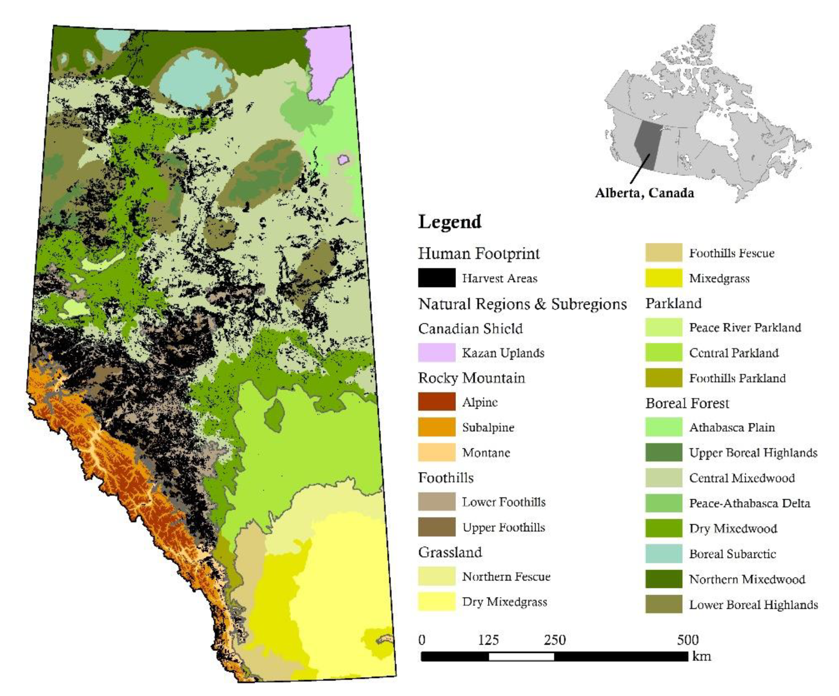
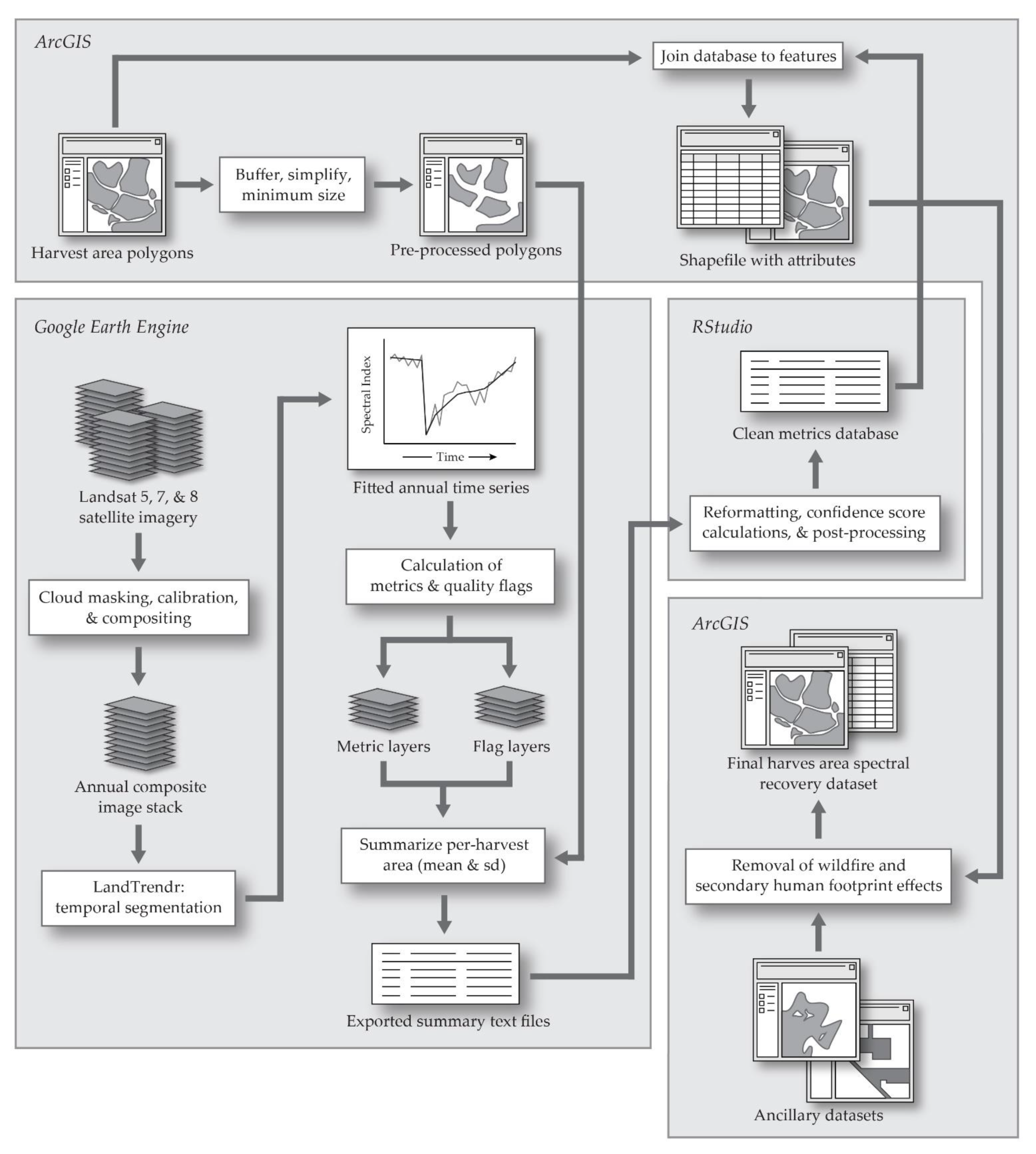
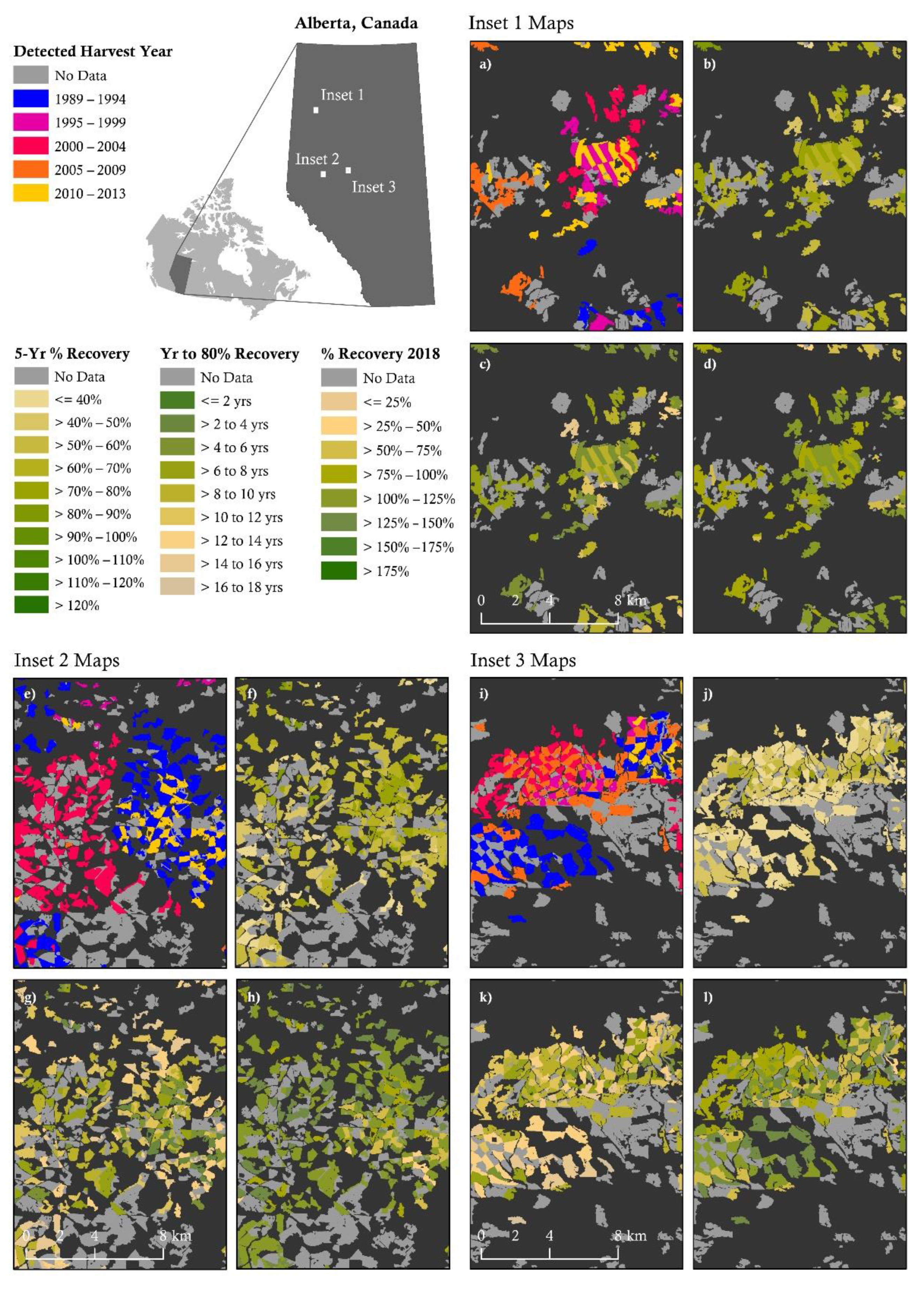
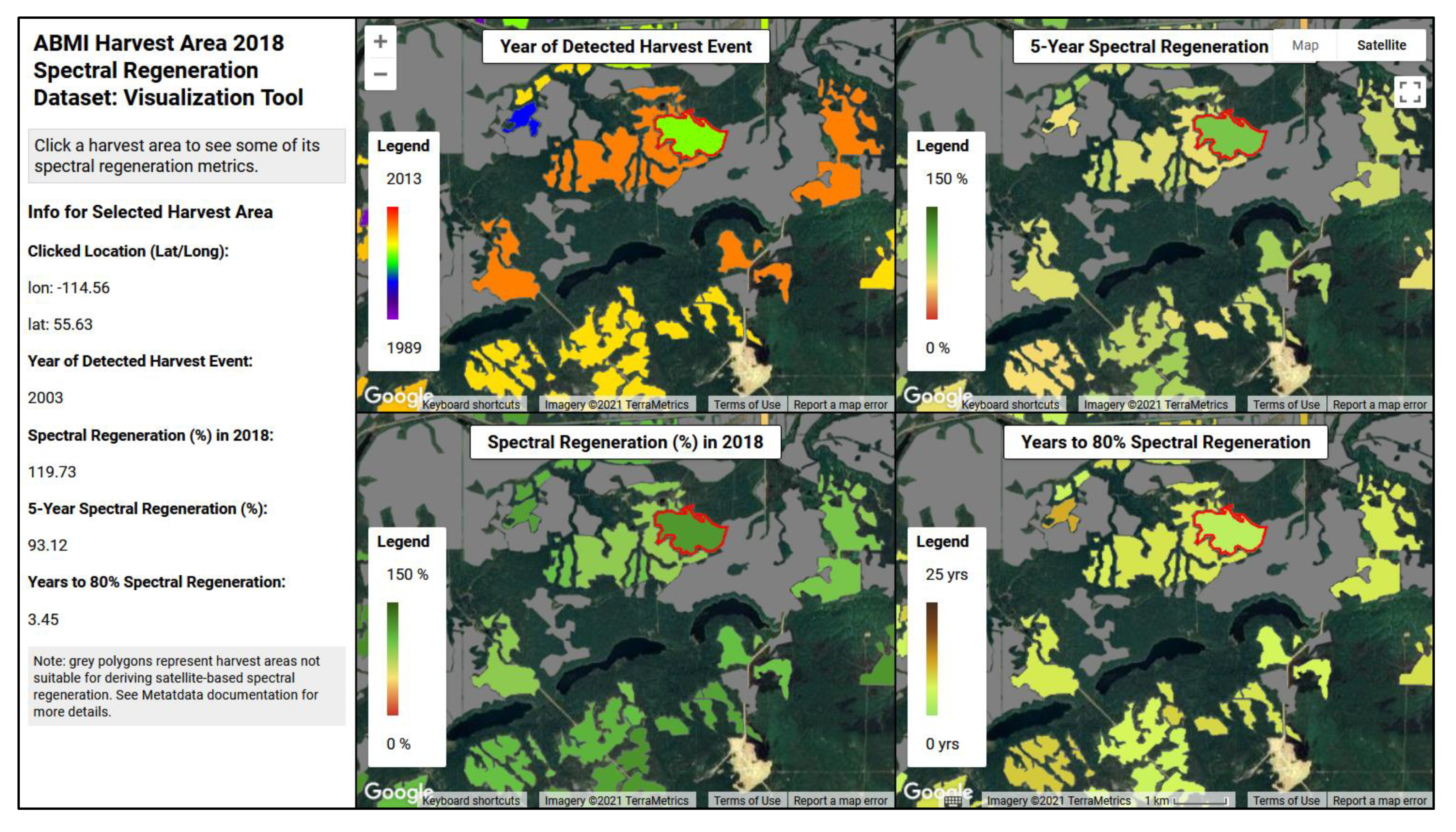
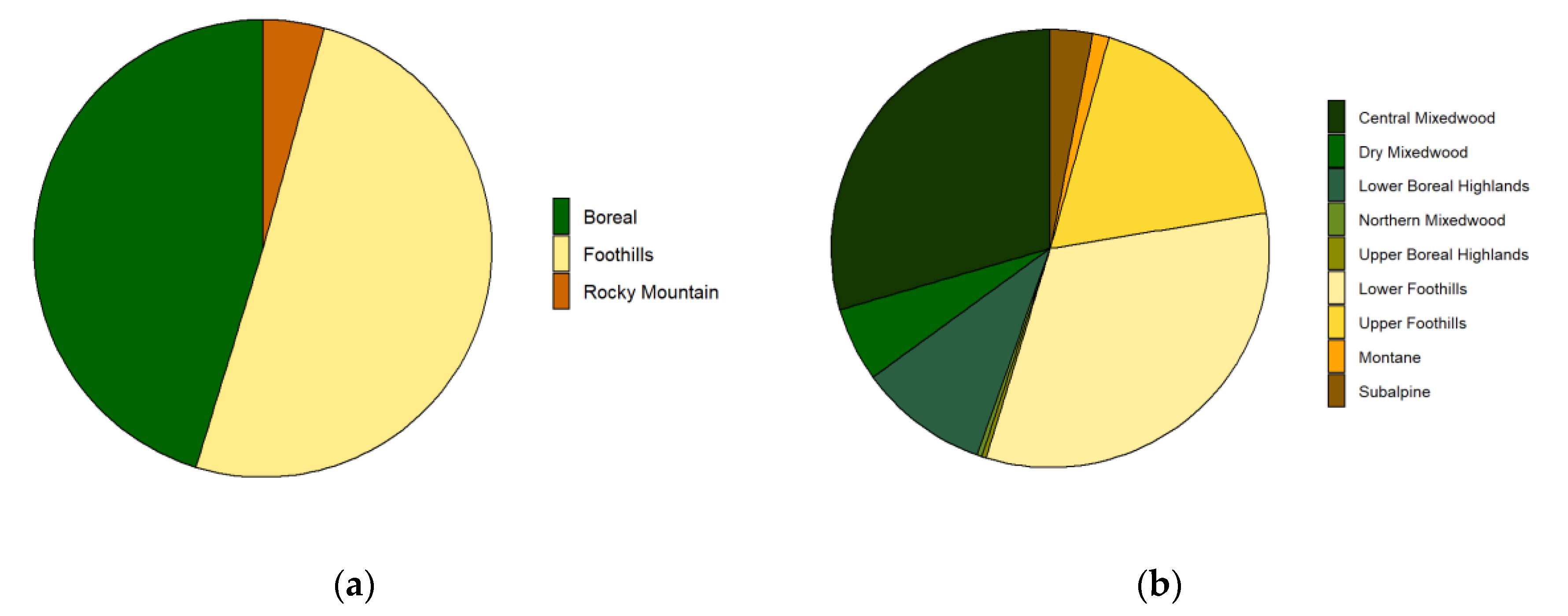
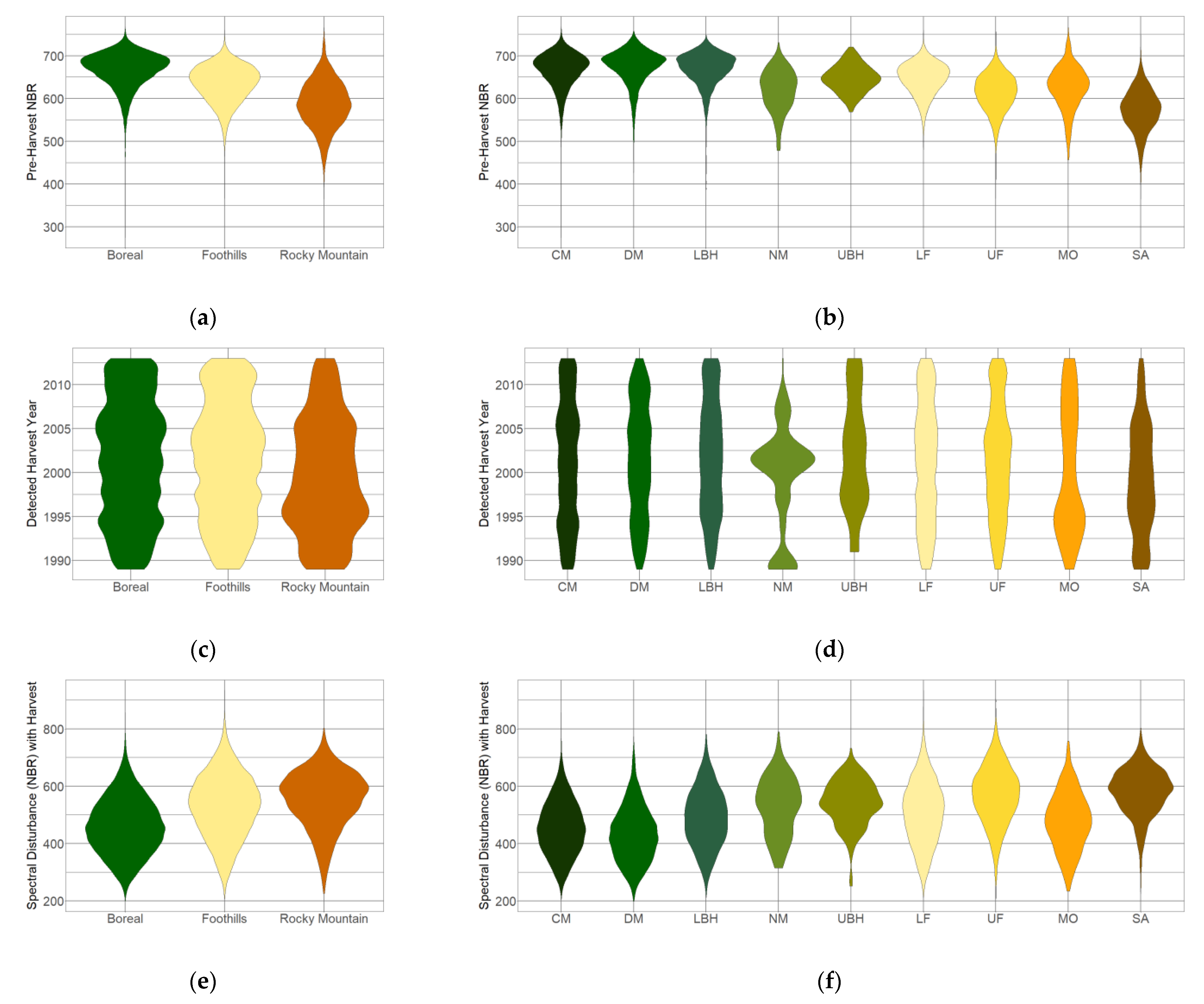
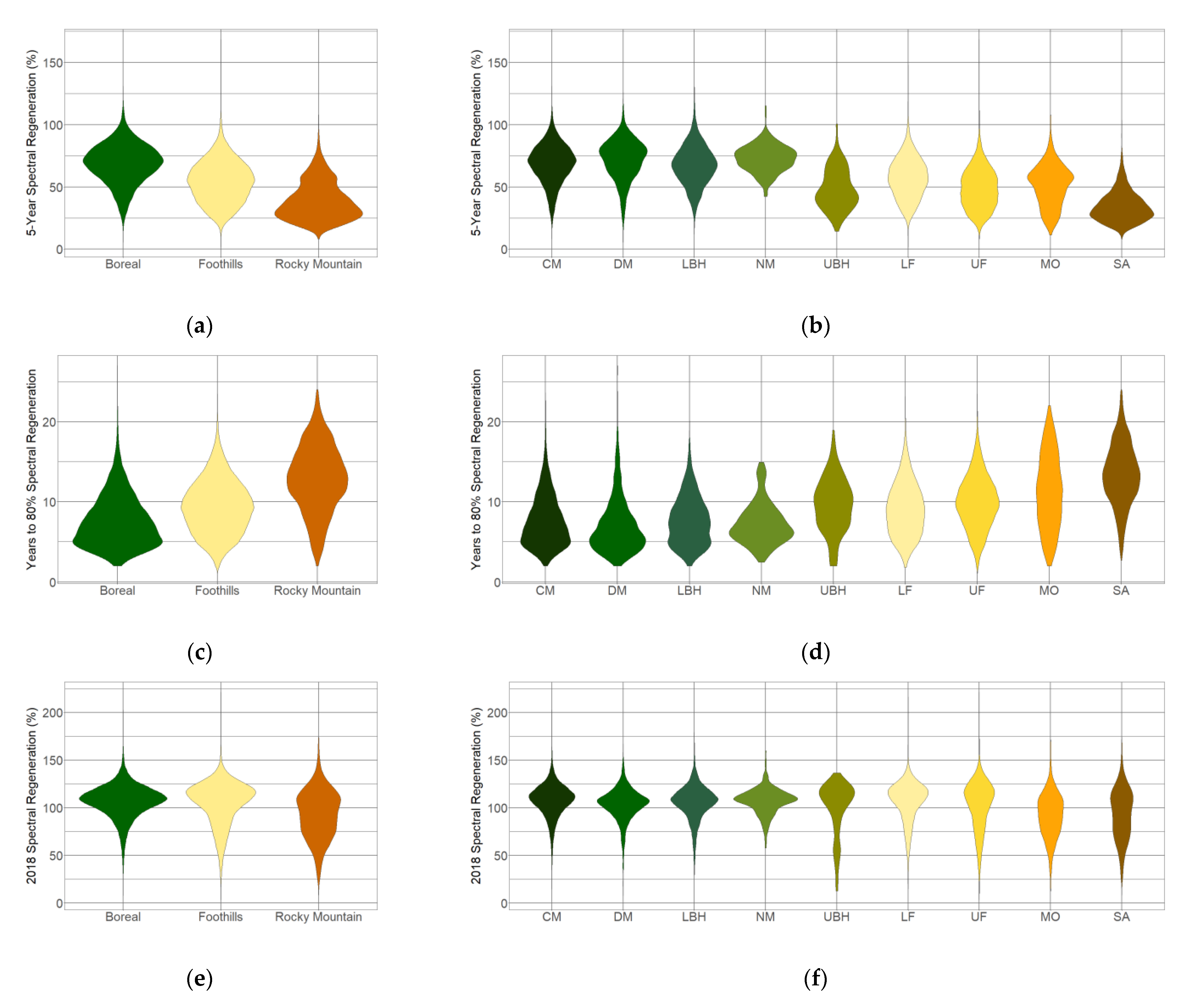
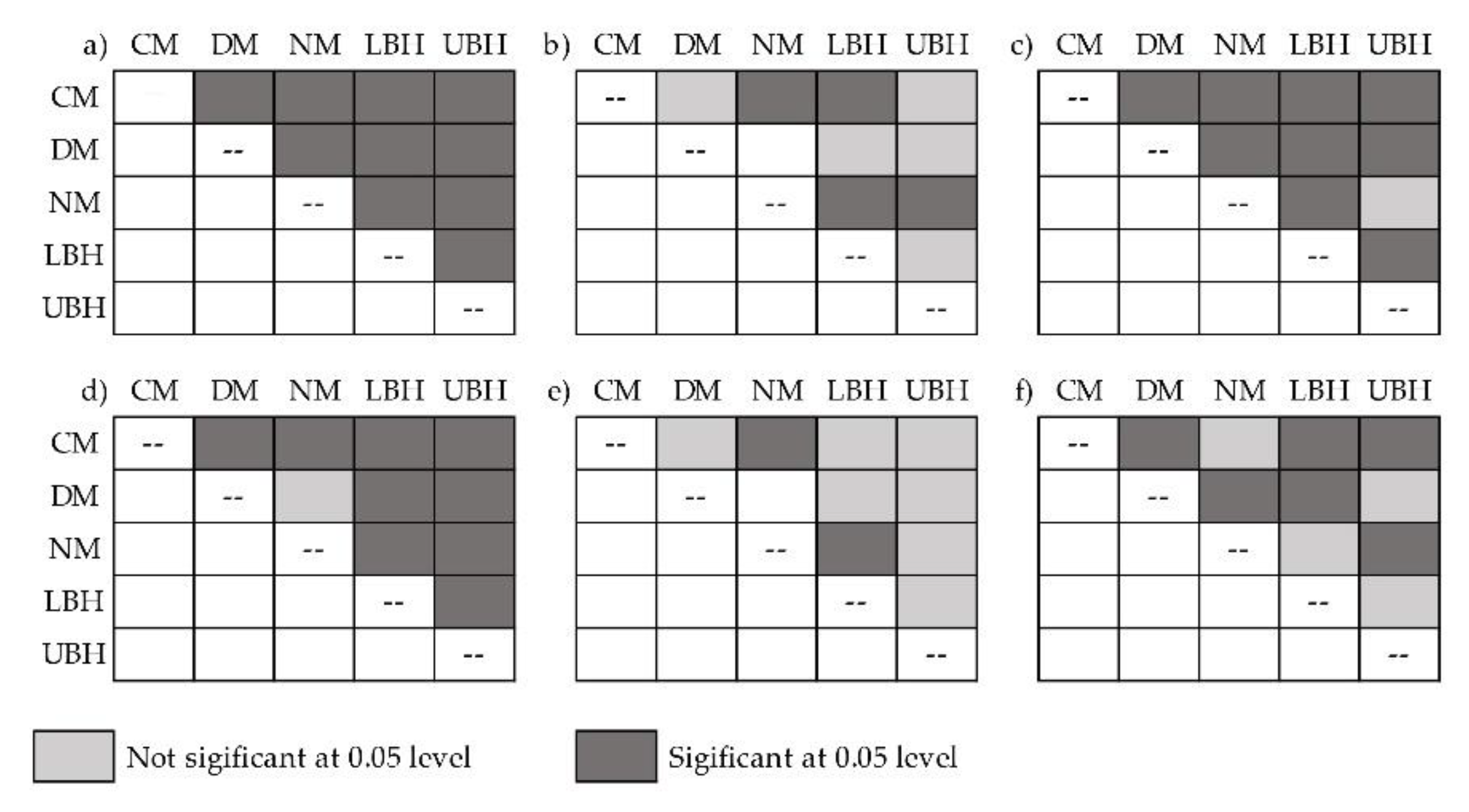
Table 1.
Description of the conditions under which pixels are flagged and removed from further analyses, and the final dataset.
Table 1.
Description of the conditions under which pixels are flagged and removed from further analyses, and the final dataset.
| Flagged Condition | Description |
|---|---|
| No harvest detected | When an inter-annual drop of 0.2 NBR units is not detected within a time series |
| No recovery detected | When a post-harvest increase in NBR values is not detected (e.g., reflecting permanent human footprint features such as a well pad within a harvest-area polygon) |
| Multiple disturbance events detected | When more than one inter-annual drop in NBR values is detected at least three years apart (one must be a drop greater than 0.2 NBR units, while additional drops must be greater than 0.175 NBR units) |
| Harvest out of date range | When a harvest is detected within an NBR time series, but is within five years of the start of the time series, or when the beginning of the recovery period is within five years of the end of the time series |
Table 2.
Summary of statistics describing the harvest and recovery metrics extracted for the 57,797 harvest areas in the final dataset. See Materials and Methods section for symbol definitions.
Table 2.
Summary of statistics describing the harvest and recovery metrics extracted for the 57,797 harvest areas in the final dataset. See Materials and Methods section for symbol definitions.
| Metric | Units | Minimum | Maximum | Mean | Stand. Dev. | n |
|---|---|---|---|---|---|---|
| NBRpreDistb | NBR | 0.275 | 0.768 | 0.647 | 47.53 | 57,797 |
| Harvestyr | year | 1989 | 2013 | 2001.25 | 6.70 | 57,797 |
| Recovstart | year | 1989 | 2013 | 2001.51 | 6.69 | 57,797 |
| Recovlag | no. years | 1 | 9.50 | 1.26 | 0.43 | 57,797 |
| NBRtotDistb | NBR | 0.199 | 0.934 | 0.501 | 0.110 | 57,797 |
| Recov%5yrr | % | 1.86 | 168.47 | 59.90 | 18.31 | 57,797 |
| Y2R | no. years | 1.08 | 27.00 | 8.70 | 3.56 | 57,238 |
| Recov%endTS | % | 3.59 | 221.28 | 105.20 | 20.87 | 57,797 |
Publisher’s Note: MDPI stays neutral with regard to jurisdictional claims in published maps and institutional affiliations. |
© 2021 by the authors. Licensee MDPI, Basel, Switzerland. This article is an open access article distributed under the terms and conditions of the Creative Commons Attribution (CC BY) license (https://creativecommons.org/licenses/by/4.0/).
Share and Cite
MDPI and ACS Style
Hird, J.N.; Kariyeva, J.; McDermid, G.J. Satellite Time Series and Google Earth Engine Democratize the Process of Forest-Recovery Monitoring over Large Areas. Remote Sens. 2021, 13, 4745. https://doi.org/10.3390/rs13234745
AMA Style
Hird JN, Kariyeva J, McDermid GJ. Satellite Time Series and Google Earth Engine Democratize the Process of Forest-Recovery Monitoring over Large Areas. Remote Sensing. 2021; 13(23):4745. https://doi.org/10.3390/rs13234745
Chicago/Turabian StyleHird, Jennifer N., Jahan Kariyeva, and Gregory J. McDermid. 2021. "Satellite Time Series and Google Earth Engine Democratize the Process of Forest-Recovery Monitoring over Large Areas" Remote Sensing 13, no. 23: 4745. https://doi.org/10.3390/rs13234745
Note that from the first issue of 2016, this journal uses article numbers instead of page numbers. See further details here.