
Feasibility Study on Estimation of Sea Ice Drift from KOMPSAT-5 and COSMO-SkyMed SAR Images


 , , , ,
  , and
, and
Abstract
:1. Introduction
2. Materials and Methods
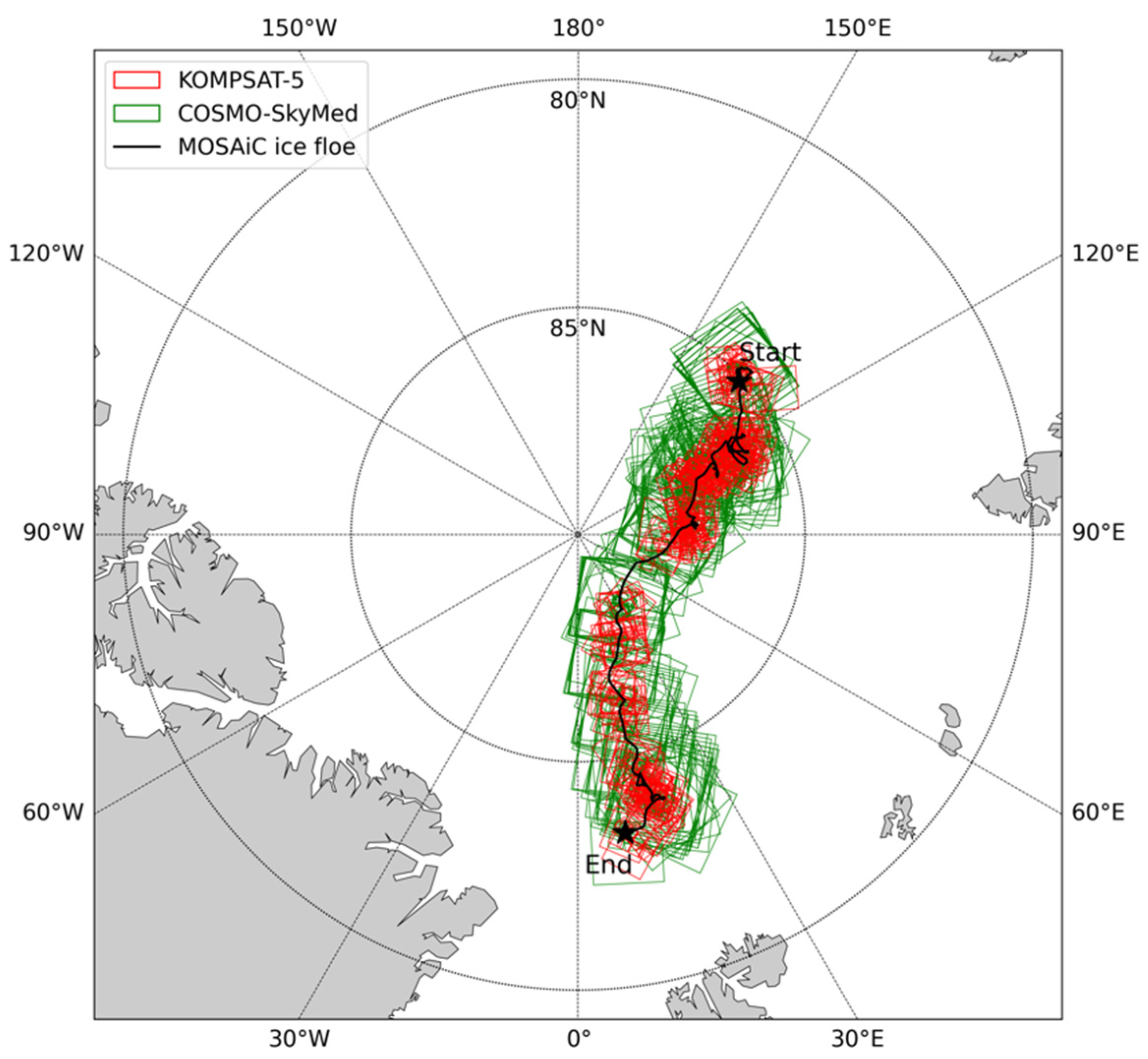
2.1. KOMPSAT-5 Dataset
2.2. COSMO-SkyMed Dataset
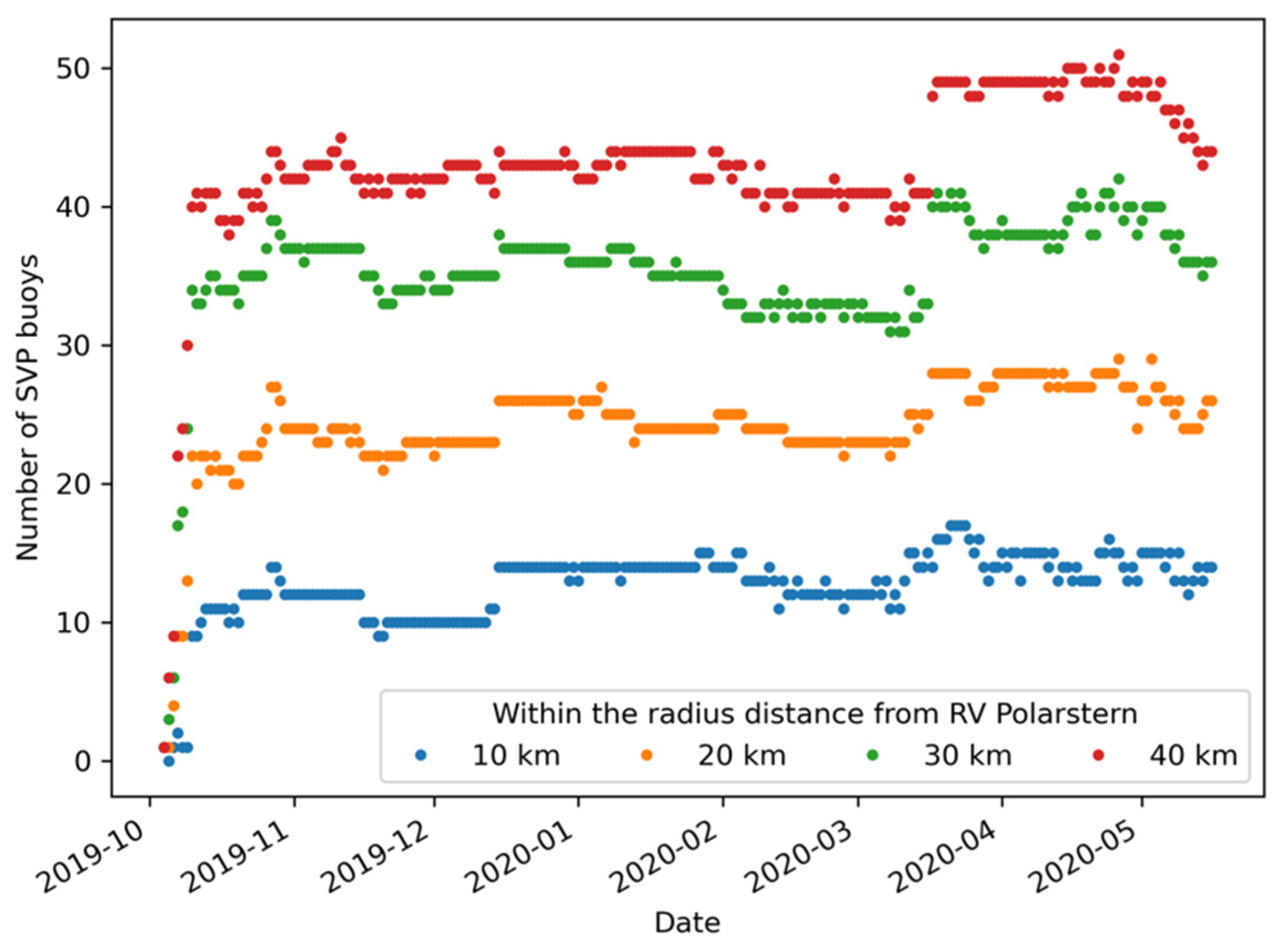
2.3. MOSAiC Distributed Network Buoys
2.4. Sea Ice Drift Retrieval
3. Results
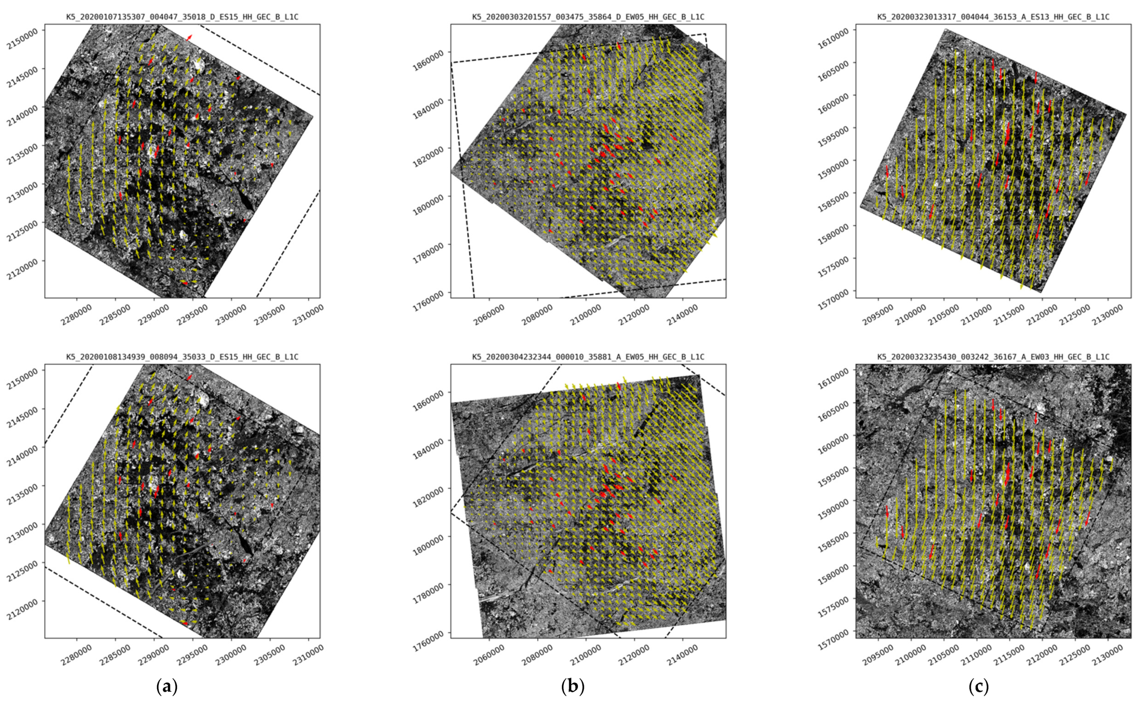
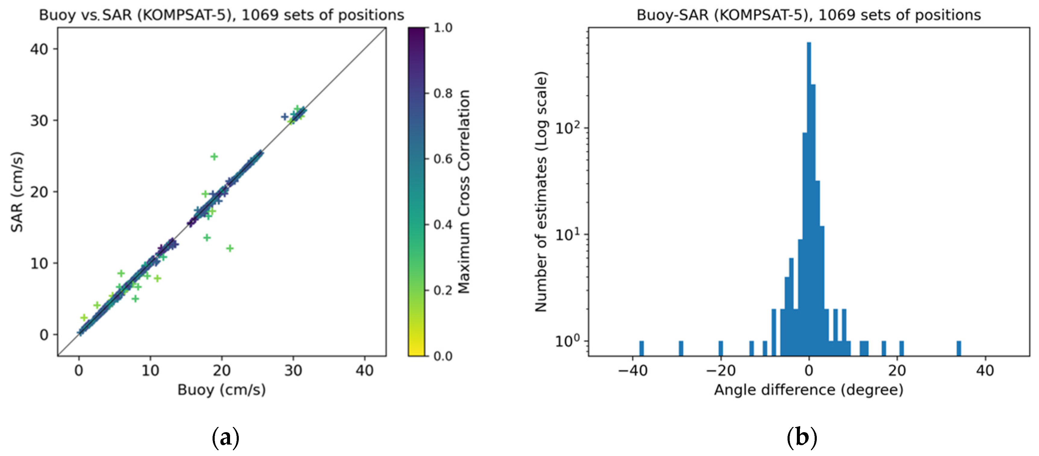
3.1. KOMPSAT-5
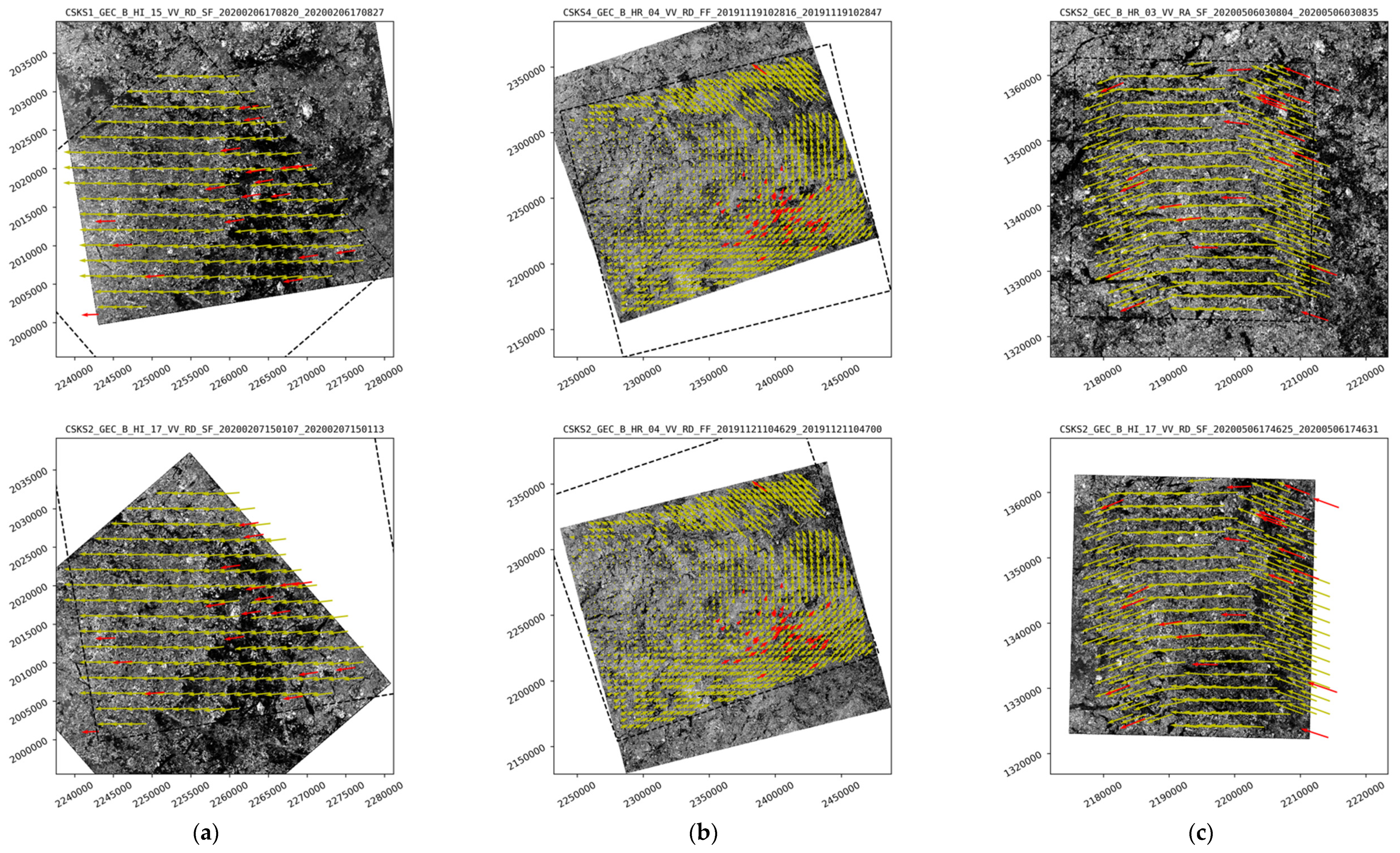
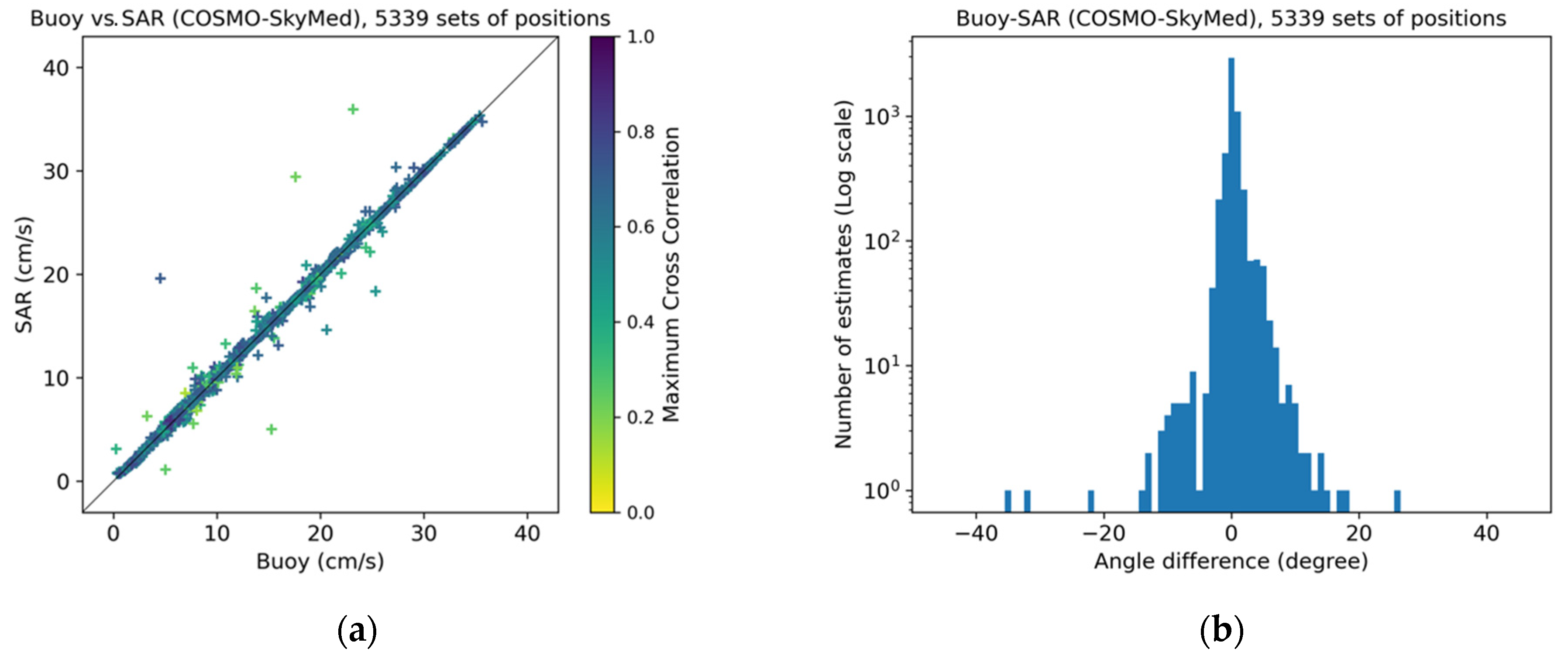
3.2. COSMO-SkyMed
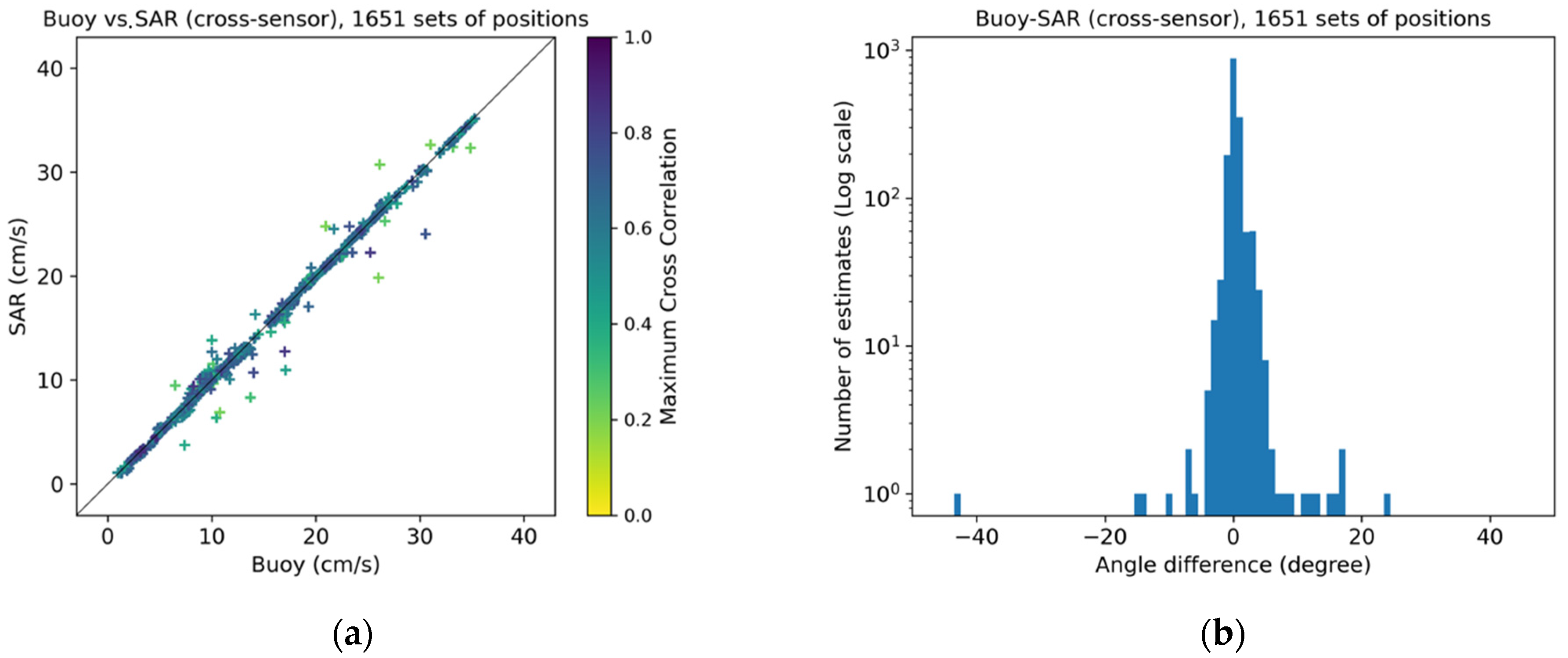
3.3. Cross-Sensor (KOMPSAT-5 and COSMO-SkyMed)
4. Discussion
5. Conclusions
Author Contributions
Funding
Institutional Review Board Statement
Informed Consent Statement
Data Availability Statement
Acknowledgments
Conflicts of Interest
References
- Serreze, M.C.; Barrett, A.P.; Slater, A.G.; Steele, M.; Zhang, J.; Trenberth, K.E. The large-scale energy budget of the Arctic. J. Geophys. Res. 2007, 112, D11122. [Google Scholar] [CrossRef] [Green Version]
- Vihma, T. Effects of Arctic Sea Ice Decline on Weather and Climate: A Review. Surv. Geophys. 2014, 35, 1175–1214. [Google Scholar] [CrossRef] [Green Version]
- Maykut, G.A. The Surface Heat and Mass Balance. In The Geophysics of Sea Ice; Untersteiner, N., Ed.; NATO ASI Series (Series B: Physics); Springer: Boston, MA, USA, 1986. [Google Scholar] [CrossRef]
- Curry, J.A.; Schramm, J.L.; Ebert, E.E. Sea Ice-Albedo Climate Feedback Mechanism. J. Clim. 1995, 8, 240–247. [Google Scholar] [CrossRef]
- Thorndike, A.S.; Rothrock, D.A.; Maykut, G.A.; Colony, R. The thickness distribution of sea ice. J. Geophys. Res. 1975, 80, 4501–4513. [Google Scholar] [CrossRef]
- Kwok, R.; Cunningham, G.F. Contributions of growth and deformation to monthly variability in sea ice thickness north of the coasts of Greenland and the Canadian Arctic Archipelago. Geophys. Res. Lett. 2016, 43, 8097–8105. [Google Scholar] [CrossRef]
- Tschudi, M.; Meier, W.N.; Stewart, J.S.; Fowler, C.; Maslanik, J. Polar Pathfinder Daily 25 km EASE-Grid Sea Ice Motion Vectors, Version 4; NASA National Snow and Ice Data Center Distributed Active Archive Center: Boulder, CO, USA, 2019. Available online: https://nsidc.org/data/NSIDC-0116/versions/3 (accessed on 15 July 2021). [CrossRef]
- Lindsay, R.; Schweiger, A. Arctic sea ice thickness loss determined using subsurface, aircraft, and satellite observations. Cryosphere 2015, 9, 269–283. [Google Scholar] [CrossRef] [Green Version]
- Spreen, G.; Kwok, R.; Menemenlis, D. Trends in Arctic sea ice drift and role of wind forcing: 1992–2009. Geophys. Res. Lett. 2011, 38, L19501. [Google Scholar] [CrossRef] [Green Version]
- Rampal, P.; Weiss, J.; Marsan, D. Positive trend in the mean speed and deformation rate of Arctic sea ice, 1979–2007. J. Geophys. Res. 2009, 114, C05013. [Google Scholar] [CrossRef]
- Farooq, U.; Rack, W.; McDonald, A.; Howell, S. Long-Term Analysis of Sea Ice Drift in the Western Ross Sea, Antarctica, at High and Low Spatial Resolution. Remote Sens. 2020, 12, 1402. [Google Scholar] [CrossRef]
- Rampal, P.; Bouillon, S.; Ólason, E.; Morlighem, M. neXtSIM: A new Lagrangian sea ice model. Cryosphere 2016, 10, 1055–1073. [Google Scholar] [CrossRef] [Green Version]
- Rampal, P.; Dansereau, V.; Olason, E.; Bouillon, S.; Williams, T.; Korosov, A.; Samaké, A. On the multi-fractal scaling properties of sea ice deformation. Cryosphere 2019, 13, 2457–2474. [Google Scholar] [CrossRef] [Green Version]
- Emery, W.J.; Fowler, C.W.; Hawkins, J.; Preller, R.H. Fram Strait satellite image-derived ice motions. J. Geophys. Res. 1991, 96, 4751–4768. [Google Scholar] [CrossRef]
- Agnew, T.; Le, H.; Hirose, T. Estimation of large-scale sea-ice motion from SSM/I 85.5 GHz imagery. Ann. Glaciol. 1997, 25, 305–311. [Google Scholar] [CrossRef] [Green Version]
- Haarpaintner, J. Arctic-wide operational sea ice drift from enhanced-resolution QuikSCAT/SeaWinds scatterometry and its validation. IEEE Trans. Geosci. Remote Sens. 2006, 44, 102–107. [Google Scholar] [CrossRef]
- Kwok, R.; Curlander, J.C.; McConnell, R.; Pang, S. An Ice Motion Tracking System at the Alaska SAR Facility. IEEE J. Ocean. Eng. 1990, 15, 44–54. [Google Scholar] [CrossRef]
- Thomas, M.; Geiger, C.A.; Kambhamettu, C. High resolution (400 m) motion characterization of sea ice using ERS-1 SAR imagery. Cold Reg. Sci. Technol. 2008, 52, 207–223. [Google Scholar] [CrossRef]
- Hollands, T.; Dierking, W. Performance of a multiscale correlation algorithm for the estimation of sea-ice drift from SAR images: Initial results. Ann. Glaciol. 2011, 52, 311–317. [Google Scholar] [CrossRef] [Green Version]
- Komarov, A.S.; Barber, D.G. Sea Ice Motion Tracking from Sequential Dual-Polarization RADARSAT-2 Images. IEEE Trans. Geosci. Remote Sens. 2014, 52, 121–136. [Google Scholar] [CrossRef]
- Korosov, A.A.; Rampal, P. A Combination of Feature Tracking and Pattern Matching with Optimal Parametrization for Sea Ice Drift Retrieval from SAR Data. Remote Sens. 2017, 9, 258. [Google Scholar] [CrossRef] [Green Version]
- Demchev, D.; Volkov, V.; Kazakov, E.; Alcantarilla, P.F.; Sandven, S.; Khmeleva, V. Sea Ice Drift Tracking from Sequential SAR Images Using Accelerated-KAZE Features. IEEE Trans. Geosci. Remote Sens. 2017, 55, 5174–5184. [Google Scholar] [CrossRef]
- Copernicus Marine Service. SEAICE_GLO_SEAICE_L4_NRT_OBSERVATIONS_011_006. Available online: https://resources.marine.copernicus.eu/?option=com_csw&view=details&product_id=SEAICE_GLO_SEAICE_L4_NRT_OBSERVATIONS_011_006 (accessed on 15 July 2021).
- Ignatenko, V.; Laurila, P.; Radius, A.; Lamentowski, L.; Antropov, O.; Muff, D. ICEYE Microsatellite SAR Constellation Status Update: Evaluation of First Commercial Imaging Modes. In Proceedings of the IGARSS 2020—IEEE International Geoscience and Remote Sensing Symposium, Virtual Symposium, Waikoloa, HI, USA , 26 September–2 October 2020; pp. 3581–3584. [Google Scholar] [CrossRef]
- Frost, A.; Jacobsen, S.; Singha, S. High resolution sea ice drift estimation using combined TerraSAR-X and RADARSAT-2 data: First tests. Proceedings of IGARSS 2017—IEEE International Geoscience and Remote Sensing Symposium, Fort Worth, TX, USA, 23–28 July 2017; pp. 342–345. [Google Scholar] [CrossRef] [Green Version]
- Krumpen, T.; Birrien, F.; Kauker, F.; Rackow, T.; von Albedyll, L.; Angelopoulos, M.; Belter, H.J.; Bessonov, V.; Damm, E.; Dethloff, K.; et al. The MOSAiC ice floe: Sediment-laden survivor from the Siberian shelf. Cryosphere 2020, 14, 2173–2187. [Google Scholar] [CrossRef]
- Korea Aerospace Research Institute (KARI). SI Imaging Services. KOMPSAT-5 Product Specifications. Available online: http://www.si-imaging.com/wp-content/uploads/2016/12/KOMPSAT-5_Standard_Products_Specifications_v1.2.pdf (accessed on 15 July 2021).
- Agenzia Spaziale Italiana (ASI). COSMO-SkyMed Mission and Products Description. Available online: https://www.asi.it/wp-content/uploads/2019/08/COSMO-SkyMed-Mission-and-Products-Description_rev3-2.pdf (accessed on 15 July 2021).
- Rabe, B.; Team MOSAiC Distributed Network. Autonomously observing coupled Arctic processes year-round: The Distributed Network of ice-tethered buoys during MOSAiC. In Proceedings of the EGU General Assembly 2021, Online, 19–30 April 2021; p. EGU21-9496. [Google Scholar] [CrossRef]
- Krumpen, T.; von Albedyll, L.; Goessling, H.F.; Hendricks, S.; Juhls, B.; Spreen, G.; Willmes, S.; Belter, H.J.; Dethloff, K.; Haas, C.; et al. The MOSAiC Drift: Ice conditions from space and comparison with previous years. Cryosphere 2021, 15, 3897–3920. [Google Scholar] [CrossRef]
- SI Imaging Services. KOMPSAT-5 Imagery Quality Report (September & October 2019). Available online: https://www.si-imaging.com/resources/?pageid=2&mod=document&keyword=KOMPSAT&uid=363 (accessed on 15 July 2021).
- SI Imaging Services. KOMPSAT-5 Imagery Quality Report (November & December 2019). Available online: https://www.si-imaging.com/resources/?pageid=2&mod=document&keyword=KOMPSAT&uid=368 (accessed on 15 July 2021).
- SI Imaging Services. KOMPSAT-5 Imagery Quality Report (January & February 2020). Available online: https://www.si-imaging.com/resources/?pageid=2&mod=document&keyword=KOMPSAT&uid=377 (accessed on 15 July 2021).
- SI Imaging Services. KOMPSAT-5 Imagery Quality Report (March & April 2020). Available online: https://www.si-imaging.com/resources/?pageid=1&mod=document&keyword=KOMPSAT&uid=385 (accessed on 15 July 2021).
- Hall, R.T.; Rothrock, D.A. Sea ice displacement from Seasat synthetic aperture radar. J. Geophys. Res. 1981, 86, 11078–11082. [Google Scholar] [CrossRef] [Green Version]
- Fily, M.; Rothrock, D.A. Sea Ice Tracking by Nested Correlations. IEEE Trans. Geosci. Remote Sens. 1987, GE-25, 570–580. [Google Scholar] [CrossRef]
- Korosov, A.A.; Hansen, M.W.; Dagestad, K.-F.; Yamakawa, A.; Vines, A.; Riechert, M. Nansat: A Scientist-Orientated Python Package for Geospatial Data Processing. J. Open Res. Softw. 2016, 4. [Google Scholar] [CrossRef] [Green Version]
- Crosby, D.S.; Breaker, L.C.; Gemmill, W.H. A Proposed Definition for Vector Correlation in Geophysics: Theory and Application. J. Atmos. Ocean. Technol. 1993, 10, 355–367. [Google Scholar] [CrossRef]
- Dierking, W. Sea ice monitoring by synthetic aperture radar. Oceanography 2013, 26, 100–111. [Google Scholar] [CrossRef]


| Parameter | KOMPSAT-5 | COSMO-SkyMed |
|---|---|---|
| Carrier frequency | 9.66 GHz (X-band) | 9.6 GHz (X-band) |
| Polarization | HH | VV |
| Imaging mode | Stripmap (1 ES), ScanSAR (2 EW) | Stripmap (3 HI), ScanSAR (4 HR) |
| Swath width | 30 km (ES), 100 km (EW) | 40 km (HI), 200 km (HR) |
| 5 GEC Pixel spacing | 1.11 m (ES), 6.25 m (EW) | 2.5 m (HI), 50 m (HR) |
| Number of image strips | 215 (ES), 101 (EW) | 374 (HI), 342 (HR) |
| 1 MCC Threshold | Number of Vectors | Drift Speed | Drift Direction | ||||
|---|---|---|---|---|---|---|---|
| Bias (cm/s) | 2 NRMSE (%) | 3ρ | Bias (Degree) | NRMSE (%) | 4ρ2 | ||
| 0.0 | 1069 | −0.052 ± 0.434 | 1.402 | 0.998 | 0.141 ± 3.720 | 2.068 | 1.994 |
| 0.2 | 1061 | −0.053 ± 0.418 | 1.352 | 0.998 | 0.266 ± 2.180 | 1.220 | 1.994 |
| 0.3 | 1042 | −0.043 ± 0.142 | 0.476 | 0.999 | 0.275 ± 1.499 | 0.846 | 1.999 |
| 0.4 | 1032 | −0.042 ± 0.130 | 0.440 | 0.999 | 0.267 ± 1.476 | 0.833 | 1.999 |
| 0.5 | 1000 | −0.042 ± 0.128 | 0.433 | 0.999 | 0.276 ± 1.495 | 0.845 | 1.999 |
| 1 MCC Threshold | Number of Vectors | Drift Speed | Drift Direction | ||||
|---|---|---|---|---|---|---|---|
| Bias (cm/s) | 2 NRMSE(%) | Bias (Degree) | NRMSE (%) | ||||
| 0.0 | 5339 | −0.009 ± 0.444 | 1.257 | 0.998 | 0.305 ± 3.127 | 1.745 | 1.996 |
| 0.2 | 5335 | −0.009 ± 0.443 | 1.254 | 0.998 | 0.302 ± 3.120 | 1.741 | 1.996 |
| 0.3 | 5305 | −0.012 ± 0.329 | 0.932 | 0.999 | 0.335 ± 1.630 | 0.924 | 1.998 |
| 0.4 | 5214 | −0.012 ± 0.317 | 0.898 | 0.999 | 0.333 ± 1.491 | 0.849 | 1.998 |
| 0.5 | 4878 | −0.011 ± 0.304 | 0.862 | 0.999 | 0.339 ± 1.458 | 0.832 | 1.998 |
| 1 MCC Threshold | Number of Vectors | Drift Speed | Drift Direction | ||||
|---|---|---|---|---|---|---|---|
| Bias (cm/s) | 2 NRMSE (%) | Bias (cm/s) | NRMSE (%) | ||||
| 0.0 | 1651 | −0.076 ± 0.505 | 1.489 | 0.997 | 0.257 ± 4.455 | 2.479 | 1.995 |
| 0.2 | 1651 | −0.076 ± 0.505 | 1.489 | 0.997 | 0.257 ± 4.455 | 2.479 | 1.995 |
| 0.3 | 1629 | −0.077 ± 0.435 | 1.289 | 0.998 | 0.297 ± 4.301 | 2.395 | 1.996 |
| 0.4 | 1595 | −0.071 ± 0.403 | 1.195 | 0.998 | 0.305 ± 4.320 | 2.406 | 1.997 |
| 0.5 | 1455 | −0.068 ± 0.356 | 1.059 | 0.998 | 0.457 ± 1.522 | 0.883 | 1.998 |
| Parameters | KOMPSAT-5 (This Study) | COSMO-SkyMed (This Study) | Cross-Sensor (This Study) | RADARSAT-2 ([20]) | Sentinel-1 ([21]) | 2 ENVISAT ASAR ([11]) |
|---|---|---|---|---|---|---|
| Pre-processed source image pixel spacing (meter) | 50 | 50 | 50 | 100 | 80 | 150 |
| RMSE in displacement (meter) | 211.53 | 210.43 | 164.11 | 428 | 286 | 1020 |
| RMSE in direction (degree) | 1.53 | 1.67 | 1.59 | 1 Unavailable | 1 Unavailable | 3.17 |
Publisher’s Note: MDPI stays neutral with regard to jurisdictional claims in published maps and institutional affiliations. |
© 2021 by the authors. Licensee MDPI, Basel, Switzerland. This article is an open access article distributed under the terms and conditions of the Creative Commons Attribution (CC BY) license (https://creativecommons.org/licenses/by/4.0/).
Share and Cite
Park, J.-W.; Kim, H.-C.; Korosov, A.; Demchev, D.; Zecchetto, S.; Kim, S.H.; Kwon, Y.-J.; Han, H.; Hyun, C.-U. Feasibility Study on Estimation of Sea Ice Drift from KOMPSAT-5 and COSMO-SkyMed SAR Images. Remote Sens. 2021, 13, 4038. https://doi.org/10.3390/rs13204038
Park J-W, Kim H-C, Korosov A, Demchev D, Zecchetto S, Kim SH, Kwon Y-J, Han H, Hyun C-U. Feasibility Study on Estimation of Sea Ice Drift from KOMPSAT-5 and COSMO-SkyMed SAR Images. Remote Sensing. 2021; 13(20):4038. https://doi.org/10.3390/rs13204038
Chicago/Turabian StylePark, Jeong-Won, Hyun-Cheol Kim, Anton Korosov, Denis Demchev, Stefano Zecchetto, Seung Hee Kim, Young-Joo Kwon, Hyangsun Han, and Chang-Uk Hyun. 2021. "Feasibility Study on Estimation of Sea Ice Drift from KOMPSAT-5 and COSMO-SkyMed SAR Images" Remote Sensing 13, no. 20: 4038. https://doi.org/10.3390/rs13204038